Optimization of Operation Parameters and Performance Prediction of Paddy Field Grader Based on a GA-BP Neural Network

Abstract

Paddy field leveling is an essential step before rice transplanting. During the operation of a paddy field grader, a common issue is the wrapping of rice straw around the blades, resulting in a low rice straw burial rate. This study focused on analyzing the operating parameters of a disc spring–tooth-combined paddy field grader. A soil–straw mechanism simulation model was created using EDEM 2021 software to simulate the field operation status. Firstly, the single-factor test was carried out, with the working speed, the working depth of the disc cutter roller, and the rotation speed of the cutter roller as the factors and the straw-buried rate (SBR) and the machine forward resistance (MFR) as the test indexes, and the parameter range was optimized. The parameters were optimized by the response surface method (RSM) and machine learning algorithms. The results indicated that the genetic algorithm–back propagation (GA-BP) neural network outperformed other optimization models in terms of prediction accuracy and stability. By utilizing the GA-BP regression model and RSM model for regression fitting, two sets of optimal parameter combinations were obtained. Verification experiments were carried out using two sets of parameter combinations. Taking the average of the experimental results, the simulation results showed that the straw burial rate was 93.47% and the forward resistance was 6487 N for the parameter combinations of RSM, and the straw burial rate was 94.86% and the forward resistance was 6352 N for the parameter combinations of GA-BP; the field experiments showed that the straw burial rate was 92.86% and the forward resistance was 6518 N for the parameter combinations of RSM, and the straw burial rate was 95.17% and the forward resistance was 6249 N for the parameter combinations of GA-BP. The results demonstrated that the GA-BP prediction model exhibited better predictive capabilities compared to the traditional RSM, providing more accurate predictions of the paddy field grader’s field operation performance.

1. Introduction

Rice straw return to the field is a crucial method of straw utilization, which can realize the synergistic improvement of soil fertility and rice yield under the premise of reducing environmental pollution and the waste of agricultural resources [1,2,3,4]. Mechanized rice straw return technology means using a straw return machine to cut off rice straw and bury it to a certain depth of the soil layer, after the subsequent microbial fermentation and maturation, the organic matter decomposes into humus to fertilize the soil, which plays a significant role in improving the soil aggregate structure [5,6]. Rice straw-returning machinery frequently encounters issues like high operating resistance and a low straw burial rate during operation [7]. Therefore, it is crucial to study and analyze the field working conditions of the paddy field grader.

The discrete element method (DEM) views soil particles as granular bodies. By analyzing the interaction between the machine and the soil system during the working process of the machine, the optimization and improvement of the working parameters of the machine can be realized, reducing the test cycles and costs [8,9,10]. Wang optimized and analyzed the field return knife roller assembly based on DEM, comparing field experiments and simulation to verify the reliability of discrete element simulation [11]. Zhang established the model of rotary tillage knife–soil–wheat straw based on DEM to explore the reliability of discrete element simulation [12]. Hadi used DEM to simulate the tillage process, optimize the working parameters of the machine, and improve the tillage speed [13] Chen used DEM to establish a soil–straw composite model of undisturbed soil under straw mulching and simulated the working process of soil tillage device [14].

In recent years, the use of artificial neural networks in modeling and solving complex relationships has become widespread due to their clear advantages in handling decentralized and nonlinear data [15,16,17]. The traditional RSM analysis method has the problem that the fitting effect is easily affected by the complexity of the problem and the sample size. The BP neural network avoids the multicollinearity problem in linear regression through the multi-layer network structure and can fit more complex nonlinear functions. [18]. Traditional machine learning models typically rely on large datasets; however, recent studies have demonstrated that smaller datasets can also be used to develop neural network models for predictive analysis [19,20,21,22]. Najet et al. used response surface methodology, artificial neural networks, and Simulink models to optimize the operating parameters for extracting capsaicin, and the results showed that artificial neural network predictions were more accurate than response surface methodology and Simulink [23]. Fetimi et al. proposed a methodology based on an optimization method based on merging an artificial neural network algorithm with PSO for predicting the optimum operating parameters for cation removal efficiency in aqueous solution [24]. MA applied four machine learning models and compared them with the response surface method. The results show that GA-BP has a better fitting effect [25].

Currently, there is limited research on optimizing machine parameters using BP neural networks. This study utilized EDEM simulation software to create a machine simulation model and simulate the field operational conditions of a disc spring–tooth-combined paddy field grader for rice straw return to the field. The single-factor test was conducted using a straw burial rate and the forward resistance of implements as indicators. Various machine learning regression models were compared for stability and accuracy, with GA-BP used to establish and optimize the model parameters. RSM and GA-BP were used to optimize the parameter inversion, resulting the parameter combinations for the field test. This study offers a foundational reference for the subsequent construction of the prediction model of machine operating parameters under complex environments in the field.

2. Materials and Methods

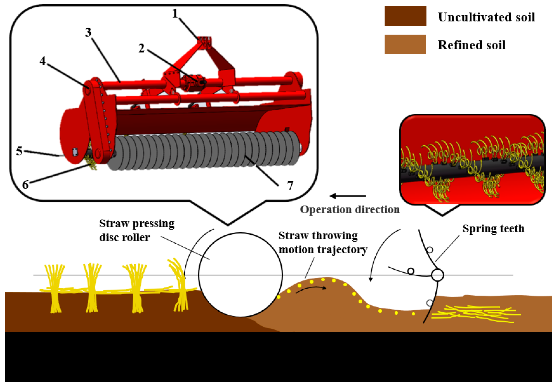
2.1. Structure and Working Principle

The disc spring–tine-combined paddy field grader utilized in this research consists primarily of a suspension device, a power input shaft, left and right gear transmission boxes, drive shafts on both sides, grass-pressing disc rollers, spring teeth, and rollers. In operation, the tractor power propels the power input shaft via the universal joint trans-mission shaft, rotating the left and right transmission shafts, and transferring power to the left and right gear transmission boxes. The left-side gear box drives the rotation of the pressure grassland disk roller, burying the rice straw and stubble. On the other hand, the right-side gear box drives the rotation of the spring elastic gear roller, mixing the slurry while burying the rice straw. The overall structure and working principle of the machine are illustrated in Figure 1. The process of determining the optimal combination of working parameters for the paddy field grader is depicted in Figure 2.

2.2. Discrete Element Simulation Modeling

To reduce the test cycle and cost, the discrete element method is usually used to simulate the operation process of the machine [8,9,10]. The soil samples were collected from the experimental field at Jilin Agricultural University, and experimental methods were used to test and analyze the basic physical properties of the soil. The contact parameters between materials are difficult to measure through conventional experimental methods. This paper sets the contact parameters between soil, cutters, and rice straw based on previously measured parameters and the related literature [26,27], as shown in

Table 1. Simulation parameter.

Factors	Value
soil–soil restitution coefficient	0.6
soil–soil static friction coefficient	0.5
soil–soil rolling friction coefficient	0.4
soil–machine restitution coefficient	0.6
soil–machine static friction coefficient	0.5
soil–machine rolling friction coefficient	0.04
soil–rice straw restitution coefficient	0.6
soil–rice straw static friction coefficient	0.5
soil–rice straw rolling friction coefficient	0.2
rice straw–rice straw restitution coefficient	0.6
rice straw–rice straw static friction coefficient	0.5
rice straw–rice straw rolling friction coefficient	0.01
rice straw–machine restitution coefficient	0.6
rice straw–machine static friction coefficient	0.3
rice straw–machine rolling friction coefficient	0.01
JKR surface energy	0.15

. The operating conditions of the machine designed in this article are black soil in northeast China, and the soil type is black soil. The reference literature sets the paddy soil particles as spherical, and the particle radius is 7 mm [28]. Due to the large soil moisture content and surface adhesion, considering that the viscous force existing between wet particles will have an impact on particle movement, the Hertz–Mindlin with JKR contact model was selected as the model between soil particles and rice straw and between soil and rice straw [29]. The three-dimensional model of the work equipment was created using Solid Works 2024 software with equal proportions and then imported into the EDEM software. To adapt to the size of the equipment, a soil box with a length × width × height of 2000 mm × 2800 mm × 200 mm was set. The straw stubble was modeled using the Bonding V2 model to accurately simulate its flexible nature [30]. The spherical particles with a radius of 5 mm were used, and the contact radius was set to 5.5 mm, which was connected in turn to form the stubble model. A Polygon virtual plane was added above the soil to generate rice straw, with varying lengths of 100 mm, 200 mm, and 250 mm, composed of spherical particles with a 5 mm radius connected in sequence; the overall simulation model is shown in Figure 3.

2.3. RSM Test Design

2.3.1. Single-Factor Test

To analyze the influence of various factors on the working effect of the paddy field grader, the operating speed of the machine tool, the working depth of the disc cutter roller, and the rotation speed of the cutter roller were selected as test factors, and the straw-burying rate and the forward resistance of the machine tool were used as influencing indicators to conduct a single-factor simulation test; the single-factor experimental design is shown in

Table 2. Single-factor test coding table.

Level	Operating Speed (km/h)	Buried Depth (mm)	Working Speed (r/min)
1	2	160	200
2	2.5	170	220
3	3	180	240
4	3.5	190	260
5	4	200	280

.

The straw-burying rate refers to the percentage of the total amount of straw remaining per unit area in the field before the machine is operated and the amount of straw that is buried deep in the mud per unit area in the same field after the machine is operated. During the simulation test, the software post-processing function was used in the working area of the paddy field grader to establish a Grid Bin Group to record the number of all rice straws M₁ in the uncultivated surface. After the machine worked, the number of straws in the cultivated area M₂ was recorded, as shown in Figure 4. The rice straw returning rate can be obtained from Formula (1).

$$\eta ={\displaystyle \frac{M_1-M_2}{M_1}}\times 100\%$$

(1)

where η is the rice straw-burying rate, %; M₁ is the straw residue per unit area of the field before the operation, g; and M₂ is the straw residue per unit area of the field after operation, g.

2.3.2. Box–Behnken Test

To analyze the influence of the interaction between various factors on the operation effect of the paddy field grader, the Box–Behnken test was conducted using the straw-burying rate and the forward resistance of the machine as test indicators. The test factor level coding table is shown in

Table 3. Box–Behnken factor level code table.

Level Code	Operating Speed (km/h)	Buried Depth (mm)	Working Speed (r/min)
−1	2	170	240
0	2.5	180	260
1	3	190	280

.

2.4. Regression Fitting Modeling Based on Machine Learning Algorithm

The RSM is based on multiple linear regression to actively collect data to obtain a regression equation with better properties. In recent years, with the development of machine learning, compared with the regression model obtained by the RSM, the use of modern intelligent optimization algorithms can also perform good regression fitting and modeling [31]. The neural network structure includes a series of interconnected neuron layers, which are mainly composed of three layers: input layer, hidden layer, and output layer. Each layer is connected to another layer by neurons. These neurons transmit information from one layer to another. In this way, the information reaches the output layer. The Box–Behnken test results were used as the dataset for BP, GA-BP, and PSO regression fitting modeling, respectively. The dataset (20 groups) was randomly divided into a training group (14 groups, 70%), a test group (3 groups, 15%), and a verification group (3 groups, 15%).

2.4.1. BP Algorithm

In the training process, the transfer function from the input layer to the hidden layer is the Sigmoid function, and the transfer function from the hidden layer to the output layer is linear. The training algorithm adopts the nonlinear damped least squares (LM) optimization algorithm [32], and the mapminmax function is selected to normalize the input and output data.

2.4.2. GA-BP Algorithm

The genetic algorithm is used to optimize the initial weights of the hidden layer and the output layer and the thresholds of the hidden layer and the output layer. The GA-BP algorithm has greater advantages in global search. Through selection, crossover, mutation, and other operations, each individual (i.e., a set of BP network parameters) evolves in the direction of higher fitness until the final standard is reached.

2.4.3. PSO Algorithm

The particle swarm optimization (PSO) algorithm, also known as the particle swarm optimization algorithm, finds the global optimal solution through the continuous iterative optimization of the particle swarm in the search space [33]. The PSO optimization algorithm first randomly generates a set of random solutions (i.e., particle swarm) and determines the fitness value of the initial particle and the individual extreme value, as well as the group extreme value through the objective function. The velocity and position of the particles are updated during the iteration process, and the optimal solution is finally found.

2.5. Data Analysis and Processing

The algorithm running platform of this study is Matlab R2020b software. The prediction performance of the machine learning model is evaluated by the determination coefficient R², mean square error (MSE), and mean absolute deviation (MAE). The larger the R², the higher the model fitting degree, the lower the MSE and MAE, and the better the model accuracy and stability.

3. Results and Discussion

3.1. Analysis of Single-Factor Experiment Results

The single-factor test results were analyzed by taking the operating speed of machine A, the depth of pressure burial B, and the speed of the knife roller C as the test factors and the straw pressure burial rate and the forward resistance of the machine as the indicators (Figure 5). The results show that with the increase in the operating speed of the machine, the straw burial rate gradually decreases, the reason may be that with the increase in the operating speed of the machine, the cutter shaft cuts the soil and reduces the effect of burial, which cannot carry out the straw burial operation in time, resulting in the gradual reduction in the burial rate, and at the same time, the resistance of the machine to move forward increases; with the increase in the depth of straw burial, the straw burial rate increases, the reason may be that with the increase in the depth of straw burial effect increases. The reason may be that as the depth increases, the effect of the straw burial increases and the forward resistance of the machine increases; as the knife roller speed increases, the straw burial rate increases, because as the knife roller speed increases, the contact stroke of the knife roller and the straw increases, and the burial rate rises, and the forward resistance of the machine increases.

3.2. Analysis of Box–Behnken Test Results

Taking the operating speed of machine A, the buried depth B, and the speed of the knife roller C as the test factors, the straw-burying rate and the forward resistance of the machine as the indicators, the Box–Behnken test design was carried out and the results were analyzed. The Box–Behnken test design and results are shown in

Table 4. Box–Behnken test design and results.

No.	A	B	C	Straw-Burying Rate (%)	Machine Forward Resistance (N)
1	−1	−1	0	89.33	5647
2	1	−1	0	86.77	7196
3	−1	1	0	95.03	6206
4	1	1	0	92.55	7251
5	−1	0	−1	87.57	6047
6	1	0	−1	88.92	7467
7	−1	0	1	95.77	6704
8	1	0	1	90.01	7420
9	0	−1	−1	87.04	6273
10	0	1	−1	93.71	6977
11	0	−1	1	95.01	6477
12	0	1	1	96.8	7294
13	0	0	0	92.4	6426
14	0	0	0	92.63	6457
15	0	0	0	92.34	6046
16	0	0	0	93.05	6498
17	0	0	0	92.91	6351
18	0	0	0	93.7	6374
19	0	0	0	92.51	6449
20	0	0	0	92.82	6362

, and ANOVO analysis for SBR and MFR is shown in

Table 5. ANOVO of Box–Behnken test on SBR.

Source	Mean Square	Degree of Freedom	Sum of Square	p-Value
Model	17.15	9	154.3100	<0.0001
A	11.1600	1	11.1600	0.0001
B	49.7000	1	49.7000	<0.0001
C	51.7700	1	51.7700	<0.0001
AB	0.0016	1	0.0016	0.9428
AC	12.6400	1	12.6400	<0.0001
BC	5.9500	1	5.9500	0.0012
A2	22.6100	1	22.6100	0.1605
B2	0.5560	1	0.5560	0.1998
C2	0.0001	1	0.0001	0.9885
Residual	0.2951	10	2.9500
Lack of fit	0.5271	3	1.5800	0.1265
Pure error	0.1956	7	1.3700
Sum		19	157.2600

and

Table 6. ANOVO of Box–Behnken test on MFR.

Source	Mean Square	Degree of Freedom	Sum of Square	p-Value
Model	513,400	9	4,620,000	<0.0001
A	2,797,000	1	2,797,000	<0.0001
B	569,800	1	569,800	0.0010
C	159,900	1	159,900	0.0349
AB	63,504	1	63,504	0.1553
AC	123,900	1	123,900	0.0574
BC	3192.25	1	3192.25	0.7375
A2	22.6100	1	22.6100	0.0413
B2	147,200	1	147,200	0.7493
C2	2900.16	1	2900.16	0.0009
Residual	591,400	10	268,800
Lack of fit	26,878.76	3	130,000	0.1775
Pure error	19,820.84	7	138,700
Sum		19	4,889,000

.

The variance analysis of the BB test results was carried out to explore the influence of each factor and the interaction of each factor on the response index. The variance analysis of the straw-burying rate showed that the model p < 0.001, indicating that there was a significant relationship between the response value and the parameters. Among them, A (machine operating speed), B (buried depth), C (working speed), AC, BC interaction term, and A² all had extremely significant effects on straw compaction rate. The coefficient of determination of the model, R² = 0.9872, and the calibrated coefficient of determination, Adjusted R² = 0.9707, were close to 1. The model misfit term was 0.0671 (>0.05), indicating that the model fits well and can be used for subsequent prediction analysis. The variance analysis of the forward resistance shows that the model p < 0.001, indicating that there is a significant relationship between the response value and the parameters. Among them, A, B, and C² all have extremely significant effects on the forward resistance, and the interaction terms of C and A² have significant effects on the forward resistance. The coefficient of determination, R² = 0.9450, and the coefficient of determination, Adjusted R² = 0.8955, are both close to 1, indicating that the model is reliable and can be used for the prediction and analysis of the subsequent combination of working parameters.

Utilizing Design-Expert 13.0 software, the regression model can be analyzed to obtain the effect of the interaction of factors on SBR and MFR, in which the regression model of SBR and each significant parameter can be described as Equation (2), and the regression model of MFR and each significant parameter can be described as Equation (3). Taking the maximum straw burial rate and the minimum forward resistance as the target values, the regression equation was solved to obtain a set of parameter combinations: the machine operating speed is 2.1 km/h, the buried depth is 185 mm, and the rotation speed of the knife roller is 275 r/min.

$$\begin{gathered} SBR=92.80-1.18A+2.49B+2.54C+0.02AB-1.78AC-1.22BC \\ -2.22A^2+0.3488B^2-0.0038C^2 \end{gathered}$$

(2)

$$\begin{gathered} MFR=6370.38-591.25A+266.87B+141.38C-126.00AB-176.00AC \\ +28.25BC+179.44A^2+25.19B^2+359.69C^2 \end{gathered}$$

(3)

3.3. Machine Learning Regression Model

3.3.1. Model Comparison

The regression fitting modeling of the data is carried out by three algorithms, and the R², MSE, and MAE of the model are compared to determine the most suitable regression model for the optimization of the working parameters of the disc spring–tooth-combined paddy field grader. The key parameter settings of the three algorithm models are shown in

Table 7. Key parameter settings.

Model	Parameter	Values
BP	training steps	50
	learning rate	0.001
	number of neurons in the hidden layer	9
GA-BP	iteration times	200
	population size	100
	number of neurons in the hidden layer	9
PSO	learning rate	0.6
	Initialize the population number	50
	iteration times	100
	inertia factor	0.1

, and the model comparison results are shown in

Table 8. Model comparison.

Model	R2		MSE		MAE
	SBR	MER	SBR	MER	SBR	MER
BP	0.8645	0.9399	1.1385	14,406.5899	0.6157	78.6879
GA-BP	0.9814	0.9601	0.1394	10,681.5752	0.2281	50.3941
PSO	0.8624	0.9477	1.1031	12,531.1535	0.5486	66.0054

.

As shown in Table 4, the comparison results of the three machine learning regression models R² are GA-BP > PSO > BP, where GA-BP is a combination of the genetic algorithm and the BP neural network, PSO is a particle swarm optimization algorithm, and BP is a traditional error back propagation algorithm. In terms of the algorithm search strategy, PSO has a stronger global search ability, GA-BP combines the global search of genetic algorithm with the local search of BP, while BP relies more on the local search, which is one of the reasons why the fitting effect of GA-BP is better than PSO and BP. To evaluate the advantages and disadvantages of the algorithms more comprehensively, it is also necessary to analyze them in combination with the MSE and MAE of the model. The comparison results of the MSE of the model of the three algorithms are GA-BP < PSO < BP, and the comparison results of the MAE are GA-BP < PSO < BP. The MSE reflects the accuracy of the model, and the MAE reflects the stability of the model. The fact that the GA-BP is better than the other algorithms in both indexes indicates that the model fitted by it is both accurate and stable at the same time, and the GA-BP combines the genetic algorithm and BP neural network, which gives it the ability to search for the global optimal solution as well as carry out detailed local tuning, which may be the reason why it has the best overall performance. The MSE of PSO is inferior to GA-BP but superior to BP, which indicates that its fitting accuracy is better but its MAE is larger than that of GA-BP, and its stability is slightly poorer than that of GA-BP. PSO relies on the population to iteratively search for the global optimum but is unable to carry out detailed local tuning, which may cause its model accuracy to be inferior to that of GA-BP. This may lead to its model accuracy not being as good as GA-BP and its stability being slightly worse; meanwhile, BP relies too much on local search and easily falls into the local optimum, so its model accuracy and stability are both worse.

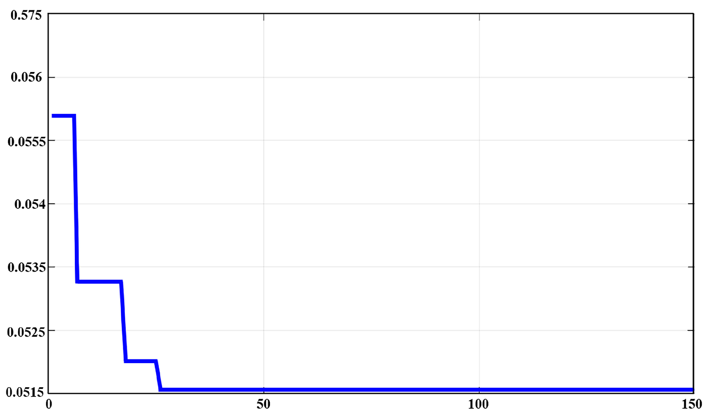
3.3.2. GA-BP Parameter Optimization

To obtain a more accurate GA-BP prediction model, the trial-and-error method was used to study the number of hidden layer neurons, population size, and iteration number of the model.

Table 9. Effect of the number of neurons on the accuracy of the model.

Value	R2		MSE		MAE
	SBR	MER	SBR	MER	SBR	MER
3	0.8180	0.8269	1.7049	38,777.4200	0.9739	124.8300
4	0.8422	0.8296	1.5617	54,210.8800	0.9190	151.3200
5	0.9149	0.8369	0.7147	39,771.5900	0.5411	141.4400
6	0.9045	0.8872	0.7203	28,001.9100	0.5606	126.7800
7	0.9392	0.8826	0.4457	22,984.2700	0.3949	96.7060
8	0.9357	0.9059	0.5056	23,214.9600	0.3449	98.8310
9	0.9677	0.9701	0.2609	9520.4390	0.2615	57.6210
10	0.9235	0.8943	0.4807	27,517.5100	0.4005	102.0500
11	0.9003	0.8834	0.7077	28,375.1100	0.5014	115.2600
12	0.8706	0.8897	0.6581	22,633.1100	0.4786	107.7600
13	0.8606	0.8716	0.8225	30,916.0500	0.6006	100.1100

shows the influence of different numbers of neurons on the accuracy of the model. With the increase in the number of neurons, the accuracy of the model increases first and then decreases.

Table 10. Effect of population size on model accuracy.

Value	R2		MSE		MAE
	SBR	MER	SBR	MER	SBR	MER
25	0.8325	0.8597	1.2412	35,402.22	0.7804	107.5754
50	0.9389	0.8997	0.4503	27,862.13	0.4843	119.3024
75	0.8608	0.9225	1.1332	18,955.8	0.6646	78.8395
100	0.9206	0.9264	0.6238	18,222.21	0.3652	88.5078
125	0.9119	0.9113	0.6929	16,788.64	0.4636	96.9820
150	0.9765	0.9701	0.2094	5652.656	0.2564	56.8173
175	0.8986	0.9044	0.7971	23,358.52	0.4933	87.8477
200	0.8385	0.9275	1.2696	17,722.82	0.5367	71.7827

shows the influence of different population sizes on the accuracy of the model. With the increase in population size, the accuracy of the model increases first and then decreases.

Table 11. Effect of different iterations on the accuracy of the model.

Value	R2		MSE		MAE
	SBR	MER	SBR	MER	SBR	MER
100	0.8589	0.8251	1.2827	42,743.3500	0.7841	137.2596
150	0.8847	0.8892	1.1515	21,678.3500	0.7043	95.9713
200	0.9862	0.9667	0.0853	6979.6340	0.1622	61.7603
250	0.8804	0.9168	0.9402	20,344.9900	0.595	80.3930
300	0.8562	0.8214	1.2565	43,864.0800	0.7221	174.7358

shows the influence of different iterations on the accuracy of the model. As the number of iterations increases, the accuracy of the model increases first and then decreases. The results show that when the number of hidden neurons is 9, the population size is 150, and the number of iterations is 200, the model has higher accuracy and better prediction ability.

3.3.3. Inversion of Parameters in GA-BP-GA

For the unknown nonlinear function, it is difficult to find the extreme value of the function only through the input and output data of the function. Therefore, combined with the nonlinear optimization ability of the genetic algorithm, the established neural network model is used as the fitness function of the genetic algorithm to optimize the operating speed of the machine, the depth of the burial, and the speed of the knife rollers by taking the maximum straw compaction rate and the minimum machine resistance as the optimization objectives. The number of evolutionary iterations of the genetic algorithm was set to 200, the population size was set to 150, the selection function was set to normGeomSelect, the coefficient was set to 0.6, the crossover coefficient was set to 2, and the mutation coefficient was set to 0.1.

Figure 6 shows the fitness curve with the evolutionary generations. Initially, the GA utilizes its population search property to make the fitness of the selected individuals plummet; subsequently, the GA carries out multiple crossover and selection processes, and the fitness of the selected individuals generates a small positive change, gradually approaching the target value; when the 27th selection generation is carried out, the fitness curve shows a state of convergence, which indicates that the difference between the predicted value and the target value is minimal. Through several selection cycles, when the number of evolutionary iterations reaches the target value of 150, the GA stops the selection and derives the individual with the closest fitness. After optimization, a set of machine working parameter combinations was obtained: machine operating speed is 2 km/h, buried depth is 190 mm, and working speed is 270 r/min.

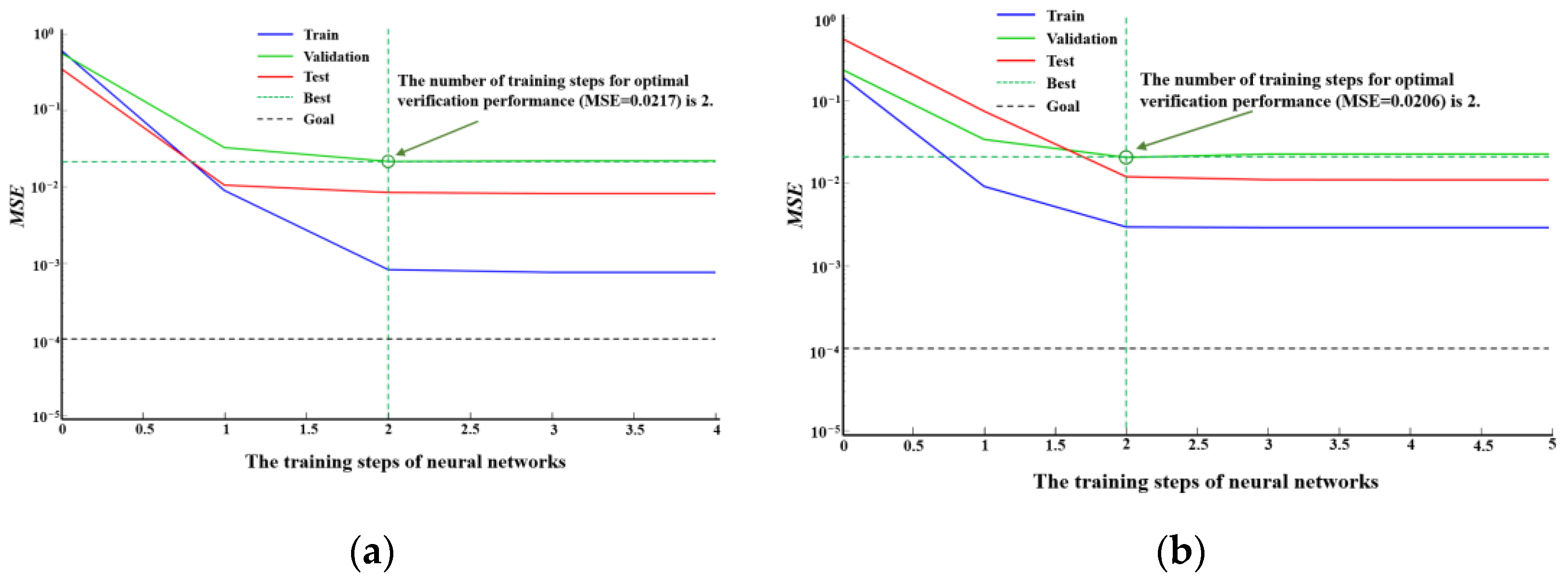
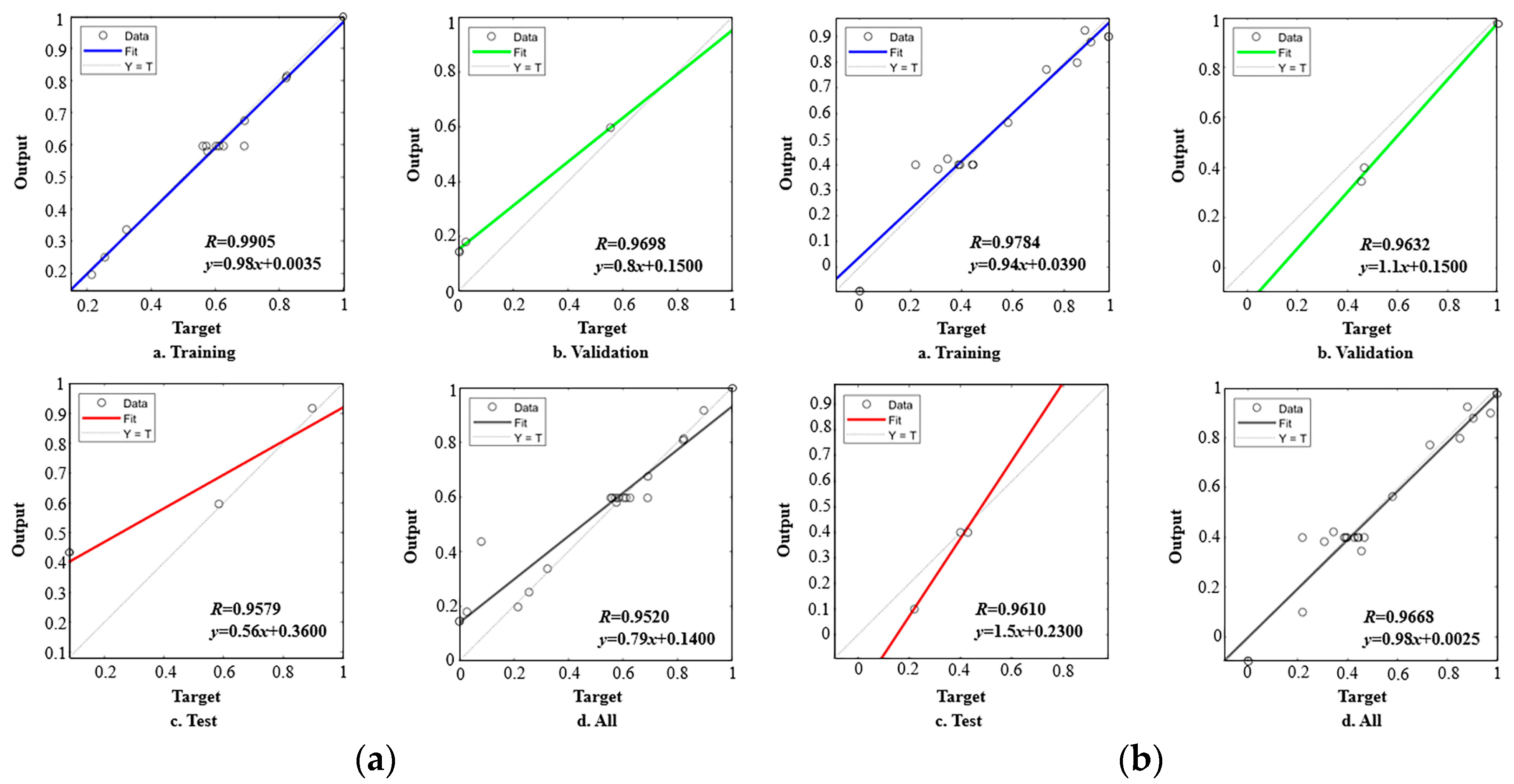
3.3.4. Model Evaluation

Using the optimized model, as shown in Figure 7, the MSE of the model is selected for performance evaluation. From the diagram, it can be seen that the MSE of the model shows a downward trend during the training process, which indicates that the effect of model fitting training data is gradually improving with the training. The best performance is obtained when training to the third step. At this time, the neural network training is basically completed, which shows that the convergence speed of GA-BP training is fast and stable, and the model can be used in the experiment. The training, verification, and testing performance of GA-BP in this study is shown in Figure 8. It can be seen from the figure that the correlation coefficient of training, verification, testing, and all data is close to 1, indicating that the model has a strong fitting effect and good generalization ability. The correlation coefficients of the data are very close, indicating that there is no obvious over-fitting or under-fitting. GA-BP performed very well in this study and obtained a model with high precision and strong generalization ability, which can be used for subsequent experimental research.

3.3.5. Experimental Verification

The parameter combinations obtained by RSM and GA-BP were used for simulation and field trials to verify the accuracy of the obtained parameter combinations, and three replicated trials were conducted. The field test site was the experimental field of Jilin Agricultural University. After 24 h of irrigation and soaking, the test was carried out after the operation plot met the standard requirements of a ‘burying grass and burying stubble tillage machine’. During the test, using a tractor as a power source to drive the paddy field grader, the pull meter was used to measure the forward resistance of the machine, and the average value of the stable operation stage of the machine was taken as the forward resistance of the machine. The straw-burying rate was calculated by measuring the straw mass ratio floating on the surface before and after the operation in the unit area. The key parameters of the operating machine are shown in

Table 12. Machine operating key parameters.

Parameters	Value
Machine size (L × W × H)/mm	3068 × 1004 × 1175
Working width/mm	2800
Number of discs	34
Number of spring teeth	76
Matching traction power requirement/kw	≥66
Hydraulic cylinder extension/mm	100
Diameter of the grass pressure disk/mm	500
Depth of burial/mm	≥160

. The field test effect is shown in Figure 9. Taking the average of the experimental results, the simulation results showed that the straw burial rate was 93.47% and the forward resistance was 6487 N for the parameter combinations of RSM, and the straw burial rate was 94.86% and the forward resistance was 6352 N for the parameter combinations of GA-BP; the field experiments showed that the straw burial rate was 92.86% and the forward resistance was 6518 N for the parameter combinations of RSM, and the straw burial rate was 95.17% and the forward resistance was 6249 N for the parameter combinations of GA-BP. The experimental results show that the parameter combination optimized by GA-BP shows a more accurate prediction performance.

4. Discussion

Compared with the traditional analysis method based on RSM, using the GA-BP algorithm to analyze and process the data. Despite its higher computational complexity and algorithm intricacy, the GA-BP model exhibits robust generalization capabilities. It can effectively address the nonlinear relationships between variables, consequently enhancing the accuracy of numerical simulations [15]. From the theoretical basis of the two models, the RSM experimental analysis method is based on statistical experimental design, constructing an approximate model (usually a quadratic polynomial model) to analyze and optimize the relationship between the response variable and independent variables. Its effectiveness relies on the accuracy of the response surface model and may not be suitable for complex systems with strong nonlinear relationships. GA-BP is a black box model. The model construction process involves the steps of population initialization, selection, crossover, and mutation of the genetic algorithm. The neural network training process optimizes model parameters and network structure to achieve optimal prediction performance. The GA-BP algorithm primarily focuses on analyzing data, especially in cases where the data relationships are unknown or exhibit a high degree of nonlinearity. Researchers in the field have utilized neural network models to compare the RSM analysis method for data analysis, with results demonstrating that the neural network model offers superior predictive capabilities. [23]. In this study, the key statistical indicators such as the determination coefficient (R²), mean absolute error (MAE), and mean square error (MSE) of the model prediction were used. The results showed that the GA-BP model showed the smallest error values in both MAE and MSE, indicating that the GA-BP model had significant advantages over the RSM method in terms of prediction accuracy and stability. These results align with previous research conducted by MA [25]. However, there are few related studies on the processing of complex data in the process of discrete element simulation operation parameter optimization. This study investigates the feasibility of utilizing GA-BP model data to analyze test results of disc spring–tooth-combined paddy field graders by comparing various neural network machine learning models and RSM analysis methods. The results demonstrate that the neural network method can be used in the field of working parameter prediction. This method can provide a reference for the optimization of related working parameters in other fields. Figure 10 shows the comparison between the measured values and the predicted values of the two models of GA-BP and RSM. The evaluation index of the GA-BP model in the figure is better than that of RSM in terms of model accuracy, stability, and fitting degree. It shows that the GA-BP algorithm has achieved a better fitting effect in this study and can construct a model with higher accuracy and smaller error, which is consistent with the research results of Bu and Nanvakenari [34,35].

5. Conclusions

In this study, through the comparison of different neural network machine learning models and RSM analysis methods, the feasibility of using GA-BP model data to analyze the test results of disc spring–tooth-combined paddy field grader is explored. The test results show that the neural network method can be used in the field of working parameter prediction. This method can provide a reference for the optimization of related working parameters in other fields. The main conclusions are as follows:

(1)

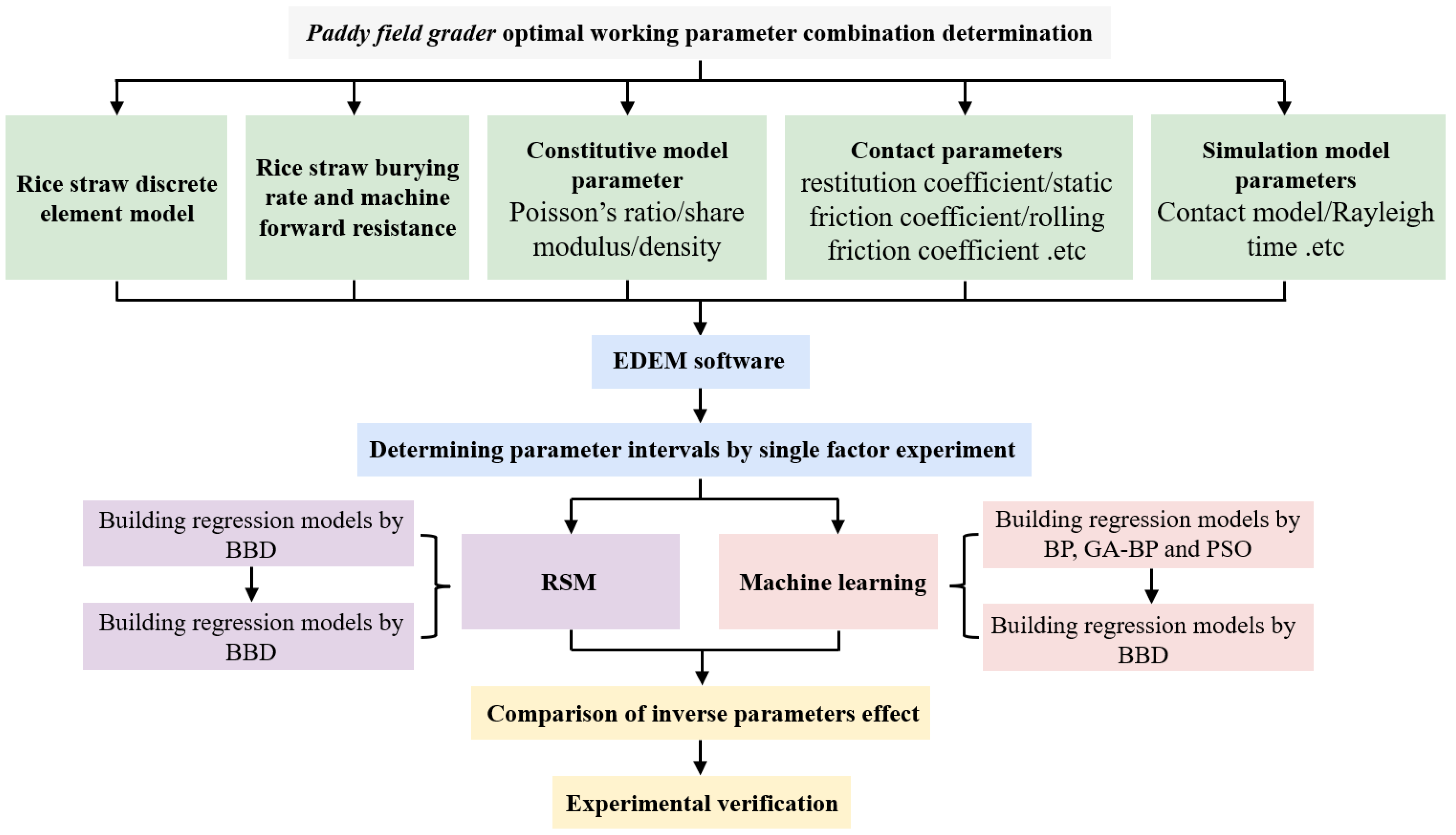
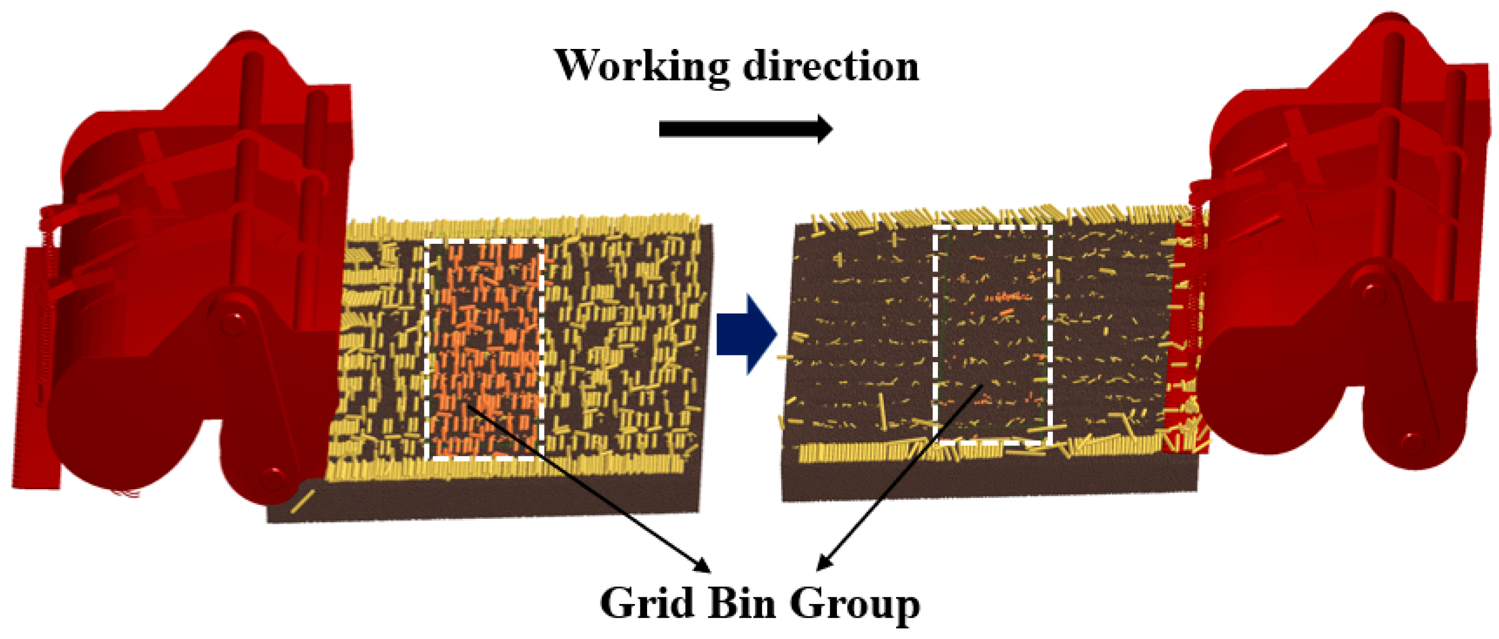
The discrete element software is used to establish a simulation model to simulate the straw-burying process of the disc spring–tooth-combined paddy field grader. The single-factor test was carried out, and the operating speed of the machine, the operating depth of the burying mechanism, and the speed of the knife roller were used as the test factors. The straw-burying rate and the forward resistance of the machine were used as indicators to optimize the range of test factors. The BB test was carried out, and the data were fitted and analyzed by RSM to explore the influence of the interaction of various factors on the operation effect.

(2)

Three machine learning regression models are compared: standard back propagation neural network (BP), back propagation neural network optimized by genetic algorithm (GA-BP), and particle swarm optimization algorithm (PSO) to evaluate their performance in the prediction of working parameters of disc spring–tooth-combined paddy field grader. The evaluation criteria include the determination coefficient (R²), mean absolute error (MAE), and mean square error (MSE). The results show that the GA-BP model has the lowest error value in both MAE and MSE indicators, and its R² value is closest to 1, indicating that the model is superior to BP and PSO models in terms of prediction accuracy and stability. The GA-BP regression model will be used as a prediction model for the working parameters of the disc spring–tooth-combined paddy field grader.

(3)

The optimized GA-BP model is used for parameter inversion, and the parameter combination obtained by GA-BP and RSM models is compared. The analysis results show that the GA-BP model is superior to the RSM model in terms of model accuracy, stability, and data fitting. The results validate the feasibility of using the GA-BP model to optimize the working parameters of the machine, and this method can provide a reference for the optimization of related working parameters in other fields as well as the calibration of discrete element simulation parameters.

References

1. Wang, Z.Y.; Chen, W.H.; Yuan, W.; Zhou, Z.P.; Liu, S.P. Nitrogen Diagnosis Model of Vegetation Indices Based on Canopy Hyperspectral Remote Sensing for Hybrid Rice. China Rice 2021, 27, 17–20+29. [Google Scholar]
2. Liu, M.H.; Li, H.Y.; Du, J.; Chen, L.; Lin, X.Y.; Zhao, H.C.; Zhang, Y.; Zhang, G.L. Effect of straw returning and increasing nitrogen of tillering fertilizer on rice yield and nitrogen uptake and utilization in cold region. J. China Agric. Univ. 2023, 28, 49–59. [Google Scholar]
3. Ge, X.L.; Qian, C.R.; Li, L.; Jiang, Y.B.; Gong, X.J.; Lv, G.Y. Effects of straw returning cooperated with fertilizer practice on yield of maize and soil quality of tillage layer. Soil Fertil. Sci. China 2021, 1, 131–136. [Google Scholar]
4. Zhai, S.L.; Xu, C.F.; Wu, Y.C.; Liu, J.; Meng, Y.L.; Yang, H.S. Long-term ditch-buried straw return alters soil carbon sequestration, nitrogen availability and grain production in a rice–wheat rotation system. Crop Pasture Sci. 2021, 72, 245–254. [Google Scholar] [CrossRef]
5. Song, J.; Huang, J.; Gao, J.S.; Wang, Y.N.; Wu, C.X.; Bai, L.Y.; Zeng, X.B. Effects of green manure planted in winter and straw returning on soil aggregates and organic matter functional groups in double cropping rice area. Chin. J. Appl. Ecol. 2021, 32, 564–570. [Google Scholar]
6. Pei, Y.N.; Lv, W.G.; Guo, T.; Bai, N.L.; Li, S.X.; Zhang, J.Q.; Zhang, H.Y.; Zhang, H.L. Effeets of straw-returning combined with application of microbial inoculants on soil aggregates and related nutrients. Chin. J. Appl. Ecol. 2023, 34, 3357–3363. [Google Scholar]
7. Sun, N.N.; Wang, X.Y.; Li, H.W.; Wang, J.; Jiang, H.; Tan, D.Y. Study on the Technology and Equipment of Rice Straw Direct Returning. J. Agric. Mech. Res. 2019, 41, 1–7. [Google Scholar]
8. Coetzee, C.J. Review: Calibration of the discrete element method. Powder Technol. 2017, 310, 104–142. [Google Scholar] [CrossRef]
9. Zhou, H.; Chen, Y.; Sadek, M.A. Modelling of soil-seed contact using the Discrete Element Method (DEM). Biosyst. Eng. 2014, 121, 56–66. [Google Scholar] [CrossRef]
10. Mustafa, U.; John, M.; Fielke, C.S. Three-dimensional discrete element modelling (DEM) of tillage: Accounting for soil cohesion and adhesione. Biosyst. Eng. 2015, 129, 298–306. [Google Scholar]
11. Wang, J.L. Discrete Element Method Deep-Buried Blade Roller Assembly Based on Optimum Design and Experimental of Rice Straw. Master’s Thesis, Northeast Agricultural University, Harbin, China, 2019. [Google Scholar]
12. Zhang, J.; Min, X.; Wei, C.; Dong, Y.; Wu, C.Y.; Zhu, J.P. Simulation Analysis and Experiments for Blade-Soil-Straw Interaction under Deep Ploughing Based on the Discrete Element Method. Agriculture 2023, 13, 136. [Google Scholar] [CrossRef]
13. Hadi, A.N.; Seyed, H.K.; Mojtaba, N.B. Weed seed burial as affected by mouldboard design parameters, ploughing depth and speed: DEM simulations and experimental validation. Biosyst. Eng. 2022, 216, 79–92. [Google Scholar]
14. Chen, G.B.; Wang, Q.J.; Li, H.W.; He, J.; Wang, X.H.; Zhang, X.Y.; He, D. Experimental research on vertical straw cleaning and soil tillage device based on Soil-Straw composite model. Comput. Electron. Agric. 2024, 216, 108510. [Google Scholar] [CrossRef]
15. Han, M. Artificial Neural Network Basis; Dalian University of Technology Press: Dalian, China, 2014. [Google Scholar]
16. Bai, H.B. Collision Damage Test and Prediction Model Establishment of Plug Seedling Based on Hanging Cup Transplanter. Master’s Thesis, Inner Mongolia Agricultural University, Hohhot, China, 2023. [Google Scholar]
17. Holzinger, A.; Fister, I., Jr.; Fister, I.; Kaul, H.-P.; Asseng, S. Human-centered ai in smart farming: Towards agriculture 5.0. IEEE Access 2024, 12, 62199–62214. [Google Scholar] [CrossRef]
18. Yan, W.Y. Noise Benefits for Image Recognition in BP Neural Networks; Nanjing University of Posts and Telecommunications: Nanjing, China, 2023. [Google Scholar]
19. Chen, L.N. Experimental Study on Coal Flotation Based RSM and BP Neural Network. Multipurp. Util. Miner. Resour. 2018, 5, 28–32. [Google Scholar]
20. Veza, I.; Spraggon, M.; Fattah, I.M.R. Response surface methodology (RSM) for optimizing engine performance and emissions fueled with biofuel: Review of RSM for sustainability energy transition. Results Eng. 2023, 18, 101213. [Google Scholar] [CrossRef]
21. Bourquin, J.; Schmidli, H.; Van, H.P. Advantages of Artificial Neural Networks (ANNs) as alternative modelling technique for data sets showing non-linear relationships using data from a galenical study on a solid dosage form. Eur. J. Pharm. Sci. 1998, 7, 5–16. [Google Scholar] [CrossRef] [PubMed]
22. Hammoudi, A.; Moussaceb, K.; Belebchouche, C. Comparison of artificial neural network (ANN) and response surface methodology (RSM) prediction in compressive strength of recycled concrete aggregates. Constr. Build. Mater. 2019, 209, 425–436. [Google Scholar] [CrossRef]
23. Najet, G.; Mahmoud, M.; Talel, B.; Kamel, N.; Ali, F. Modeling and optimization of capsaicin extraction from Capsicum annuum L. using response surface methodology (RSM), artificial neural network (ANN), and Simulink simulation. Ind. Crops Prod. 2021, 171, 113869. [Google Scholar]
24. Fetimi, A.; Dâas, A.; Benguerba, Y. Optimization and prediction of safranin-O cationic dye removal from aqueous solution by emulsion liquid membrane (ELM) using artificial neural network-particle swarm optimization (ANN-PSO) hybrid model and response surface methodology (RSM). J. Environ. Chem. Eng. 2021, 9, 105837. [Google Scholar] [CrossRef]
25. Ma, X.J.; Guo, M.J.; Tong, X.; Hou, Z.F.; Liu, H.Y.; Ren, H.Y. Calibration of Small-Grain Seed Parameters Based on a BP Neural Network: A Case Study with Red Clover Seeds. Agronomy 2023, 13, 2670. [Google Scholar] [CrossRef]
26. Zhao, J.K.; Song, W.B.; Li, J.J. Modeling and Mechanical Analysis of Rice Straw Based on Discrete Element Mechanical Model. Chin. J. Soil Sci. 2020, 51, 1086–1093. [Google Scholar]
27. Ma, Z.T.; Zhao, Z.H.; Quan, W.; Shi, F.G.; Gao, C.; Wu, M.L. Calibration of Discrete Element Parameter of Rice Stubble Straw Based on EDEM. J. Agric. Sci. Technol. 2023, 25, 103–113. [Google Scholar]
28. Tang, Z.Y.; Gong, H.; Wu, S.L.; Zeng, Z.W.; Wang, Z.Q.; Zhou, Y.H.; Fu, D.B.; Liu, C.; Cai, Y.H.; Qi, L. Modelling of paddy soil using the CFD-DEM coupling method. Soil Tillage Res. 2023, 226, 105591. [Google Scholar] [CrossRef]
29. Ding, Q.S.; Ren, J.; Belal, E.A.; Zhao, J.K.; Ge, S.Y.; Li, Y. Discrete Element Analysis of Subsoiling Process of Wet Clay Paddy Soil. Agric. Mach. 2017, 48, 38–48. [Google Scholar]
30. Zhou, J.; Sun, W.T.; Liang, Z.A. Construction of Discrete Element Flexible Model for Jerusalem Artichoke Root-Tuber at Harvest Stage. Trans. Chin. Soc. Agric. Mach. 2023, 54, 124–132. [Google Scholar]
31. Ding, X.T.; Li, K.; Hao, W.; Yang, Q.C.; Yan, F.X.; Cui, Y.J. Calibration of Simulation Parameters of Camellia oleifera SeedsBased on RSM and GA-BP-GA Optimization. Trans. Chin. Soc. Agric. Mach. 2023, 54, 139–150. [Google Scholar]
32. Gai, L. Exploration of Manufaturing Technique and Mechanical Performance Prediction of Reconsolidated Square Materials of Cotton Stalk. Master’s Thesis, Northwest A&F University, Xianyang, China, 2015. [Google Scholar]
33. Ren, K.; Jia, L.; Huang, J.T.; Wu, M. Research on cutting stock optimization of rebar engineering based on building information modeling and an improved particle swarm optimization algorithm. Dev. Built Environ. 2023, 13, 100121. [Google Scholar] [CrossRef]
34. Bu, X.Y.; Xu, Y.Q.; Zhao, M.M.; Li, D.L.; Zhou, J.H.; Wang, L.B.; Bai, J.W.; Yang, Y. Simultaneous extraction of polysaccharides and polyphenols from blackcurrant fruits: Comparison between response surface methodology and artificial neural networks. Ind. Crops Prod. 2021, 170, 113682. [Google Scholar] [CrossRef]
35. Nanvakenari, S.; Movagharejad, K.; Latifi, A. Evaluating the fluidized-bed drying of rice using response surface methodology and artificial neural network. LWT—Food Sci. Technol. 2021, 147, 111589. [Google Scholar] [CrossRef]
Figure 1. Structure and working principle of disc elastic toothed combination paddy graders (1. hanging device; 2. power input shaft; 3. left-side drive shaft; 4. left gear transmission box; 5. spring roller; 6. spring teeth; 7. grass-pressing disc roller).
Agriculture 14 01283 g001
Figure 2. Parameter combination determination flowchart.
Agriculture 14 01283 g002
Figure 3. Discrete element simulation model.
Agriculture 14 01283 g003
Figure 4. Schematic diagram of straw-burying rate determination.
Agriculture 14 01283 g004
Figure 5. Single-factor experiment results. (a) Operating speed experiment results; (b) buried depth experiment results; (c) working speed experiment results.
Agriculture 14 01283 g005
Figure 6. Fitness curve in the evolution process.
Agriculture 14 01283 g006
Figure 7. MSE performance evaluation of the model. (a) SBR; (b) MFR.
Agriculture 14 01283 g007
Figure 8. Regression analysis. (a) SBR; (b) MFR.
Agriculture 14 01283 g008
Figure 9. Field experiment.
Agriculture 14 01283 g009
Figure 10. Measured and predicted values. (a) SBR; (b) MFR.
Agriculture 14 01283 g010