Article

Early Monitoring of Maize Northern Leaf Blight Using Vegetation Indices and Plant Traits from Multiangle Hyperspectral Data

by
Anting Guo
1,
Wenjiang Huang
1,2,
Kun Wang
1,*,
Binxiang Qian
1,2 and
Xiangzhe Cheng
1,2
1
Key Laboratory of Remote Sensing and Digital Earth, Aerospace Information Research Institute, Chinese Academy of Sciences, Beijing 100094, China
2
University of Chinese Academy of Sciences, Beijing 100049, China
*
Author to whom correspondence should be addressed.
Agriculture 2024, 14(8), 1311; https://doi.org/10.3390/agriculture14081311
Submission received: 3 July 2024 / Revised: 4 August 2024 / Accepted: 7 August 2024 / Published: 8 August 2024
(This article belongs to the Section Digital Agriculture)

Abstract

:
Maize northern leaf blight (MNLB), characterized by a bottom-up progression, is a prevalent and damaging disease affecting maize growth. Early monitoring is crucial for timely interventions, thus mitigating yield losses. Hyperspectral remote sensing technology is an effective means of early crop disease monitoring. However, traditional single-angle vertical hyperspectral remote sensing methods face challenges in monitoring early MNLB in the lower part of maize canopy due to obstruction by upper canopy leaves. Therefore, we propose a multiangle hyperspectral remote sensing method for early MNLB monitoring. From multiangle hyperspectral data (−60° to 60°), we extracted and selected vegetation indices (VIs) and plant traits (PTs) that show significant differences between healthy and diseased maize samples. Our findings indicate that besides structural PTs (LAI and FIDF), other PTs like Cab, Car, Anth, Cw, Cp, and CBC show strong disease discrimination capabilities. Using these selected features, we developed a disease monitoring model with the random forest (RF) algorithm, integrating VIs and PTs (PTVI-RF). The results showed that PTVI-RF outperformed models based solely on VIs or PTs. For instance, the overall accuracy (OA) of the PTVI-RF model at 0° was 80%, which was 4% and 6% higher than models relying solely on VIs and PTs, respectively. Additionally, we explored the impact of viewing angles on model accuracy. The results show that compared to the accuracy at the nadir angle (0°), higher accuracy is obtained at smaller off-nadir angles (±10° to ±30°), while lower accuracy is obtained at larger angles (±40° to ±60°). Specifically, the OA of the PTVI-RF model ranges from 80% to 88% and the Kappa ranges from 0.6 to 0.76 at ±10° to ±30°, with the highest accuracy at −10° (OA = 88%, Kappa = 0.76). In contrast, the OA ranges from 72% to 80% and the Kappa ranges from 0.44 to 0.6 at ±40° to ±60°. In conclusion, this research demonstrates that PTVI-RF, constructed by fusing VIs and PTs extracted from multiangle hyperspectral data, can effectively monitor early MNLB. This provides a basis for the early prevention and control of MNLB and offers a valuable reference for early monitoring crop diseases with similar bottom-up progression.

1. Introduction

Maize is one of the most extensively cultivated cereal crops worldwide, ranking just behind wheat and rice in cultivation area and total production [1]. Ensuring safe maize production is crucial for national food security. Pests and diseases are the primary challenges to maize production. Nearly 600 pests and diseases significantly threaten maize, profoundly impacting its yield and quality [2]. Among these, maize northern leaf blight (MNLB), caused by Setosphaeria turcica, is one of the most prevalent and harmful diseases affecting maize [3]. In epidemic years, MNLB can reduce maize yield by 15–20%, and in severe instances, yield loss can exceed 50% [4]. Early disease monitoring is crucial for timely control measures, thereby reducing losses. Current methods for early MNLB monitoring rely on field surveys and laboratory analyses, which are labor-intensive, time-consuming, and costly [5]. These methods are increasingly insufficient to meet the growing demand for efficient disease prevention and control. In recent years, rapid advancements in hyperspectral remote sensing technology have offered a powerful tool for early crop disease monitoring. Hyperspectral remote sensing offers has high spectral resolution and narrow band range, enabling the detection of subtle spectral differences caused by early diseases [6]. Crops exhibit varying absorption and reflection properties at different wavelengths under disease stress. These distinct symptoms and optical characteristics form the basis for hyperspectral remote sensing monitoring of diseases [7]. Many researchers have used disease-sensitive features to monitor crop diseases. These features include the following. (1) Spectral bands: Researchers often select disease-sensitive spectral bands using methods such as the successive projections algorithm (SPA) and competitive adaptive reweighted sampling (CARS). For example, Gao et al. [8] selected six spectral bands highly correlated with the disease and successfully identified pre-symptomatic grapevine leafroll plants based on these bands. (2) Vegetation indices (VIs): VIs are widely used in monitoring plant diseases [9]. Established VIs effectively identify diseases, as demonstrated by Khan et al. [10], who developed a wheat powdery mildew monitoring model using hyperspectral VIs, achieving an overall accuracy (OA) of 82%. A new trend is emerging to develop VIs based on specific spectral changes caused by diseases. For example, Rumpf et al. [11] identified spectral bands closely associated with beet diseases in hyperspectral data and developed normalized difference disease spectral indices based on these bands. Consequently, they successfully identified disease symptoms using these new spectral indices. (3) Wavelet features: The continuous wavelet transform is effective for capturing subtle spectral absorption features [12]. This method converts the spectrum into wavelet features of varying amplitudes and scales [13]. Numerous studies have used wavelet features for disease monitoring. For example, Tian et al. [14] investigated the feasibility of detecting rice blast using wavelet features. The results showed identification accuracies exceeding 65%, 80%, and 95% during the asymptomatic, early, and mild infection stages, respectively. Although these features have been effective in monitoring various crop diseases, their potential for early MNLB detection remains unknown. Moreover, these features fail to fully exploit hyperspectral data potential, as VIs are constructed from only a few bands, ignoring most of the available band information.
Extracting plant traits (PTs) from hyperspectral data to monitor plant diseases is a current trend. PTs, including pigment content, water content, dry matter, canopy temperature, and vegetation structure, are closely associated with plant health and responses to biotic stressors [15]. PTs like pigments and photosynthesis typically exhibit stress responses before symptoms manifest. Therefore, the timely detection of PTs changes can effectively monitor the early stages of plant diseases. Several studies have used PTs alone for early disease monitoring. For instance, Yao et al. [16] utilized hyperspectral imaging systems to continuously monitor wheat stripe rust infection over 15 days and proposed a chlorophyll-based method for early disease detection. Their results showed that wheat stripe rust can be detected on leaves six days post-inoculation. Notably, most studies have focused on integrating PTs with spectral features to monitor vegetation diseases. This integration enhances disease characterization, thereby improving monitoring accuracy. Currently, PTs combined with spectral features are typically classified into those measured in field experiments and those generated through model simulations. Cheng et al. [17] showed that combining measured PTs with VIs, spectral features, and wavelet features enhances the early monitoring of rubber tree powdery mildew. However, using measured PTs has limitations, as the data are point-specific and unsuitable for large-scale disease monitoring. Additionally, the types of measured data are generally limited to PTs like chlorophyll and moisture. Simulated PTs extracted from spectral data include various traits [18]. For example, Zarco-Tejada et al. [19] used airborne imaging spectroscopy to extract PTs and develop a monitoring model for X. fastidiosa in olive trees. This model detected X. fastidiosa-infected olive trees with 80% OA before symptoms appeared. Furthermore, Zarco-Tejada et al. [20] successfully used this approach to differentiate X. fastidiosa-induced diseases from other abiotic stressors. Studies have also combined PTs with parameters such as thermal imaging data and chlorophyll fluorescence to monitor vegetation diseases. Poblete et al. [21] successfully distinguished olive trees infected with Xylella fastidiosa from those infected with Verticillium dahliae using a machine learning approach integrating these three features. The aforementioned studies primarily focused on monitoring forest diseases using a combination of PTs and VIs. However, the effectiveness of this approach for the early monitoring of crop diseases, particularly MNLB, remains uncertain.
Currently, the remote sensing monitoring of crop diseases primarily relies on single-angle vertical observation. This method effectively monitors diseases like wheat stripe rust, fusarium head blight, and rice blast on the upper canopy of crops but has limitations for diseases in the lower canopy. Diseases such as MNLB and wheat powdery mildew typically exhibit a bottom-up infection pattern, initially affecting the lower canopy and gradually spreading to the upper canopy as severity increases [22]. Therefore, due to occlusion by upper canopy leaves, single-angle vertical remote sensing may struggle to detect early stages of MNLB. Multiangle remote sensing uses sensors to conduct the non-contact observations of the same target from two or more directions [23,24]. Compared to single-angle vertical observation, multiangle remote sensing captures the three-dimensional structure of crops and information from lower canopy leaves [25,26]. In recent years, multiangle remote sensing has proven successful in crop disease monitoring. He et al. [22] developed a new wheat powdery mildew monitoring index (RPMI) based on multiangle hyperspectral data. This index improves monitoring accuracy for powdery mildew severity at a single angle and provides stable accuracy within the range of 0° to +30°, thus expanding the application scope of remote sensing. Song et al. [27] employed multiangle hyperspectral data combined with various machine learning methods to construct a wheat powdery mildew monitoring model. Their results indicated that the CARS-ELM model achieved better performance (R2 > 0.8 for each angle). The aforementioned crop disease monitoring using multi-angle remote sensing technology that relies on spectral features, and no research has yet incorporated PTs.
In conclusion, although multiangle remote sensing has advantages for acquiring lower canopy information, its effectiveness in early MNLB monitoring remains uncertain, especially utilizing PTs. Therefore, in this study, we primarily used PTs and VIs extracted from multiangle hyperspectral data to monitor early MNLB. The specific objectives were to: (1) evaluate the capability of PTs and VIs from hyperspectral data to differentiate between early infected and healthy maize; (2) develop and evaluate an early monitoring model for MNLB, integrating PTs and VIs, constructed using a random forest (RF) algorithm; and (3) assess the impact of different angles on the model’s performance.

2. Materials and Methods
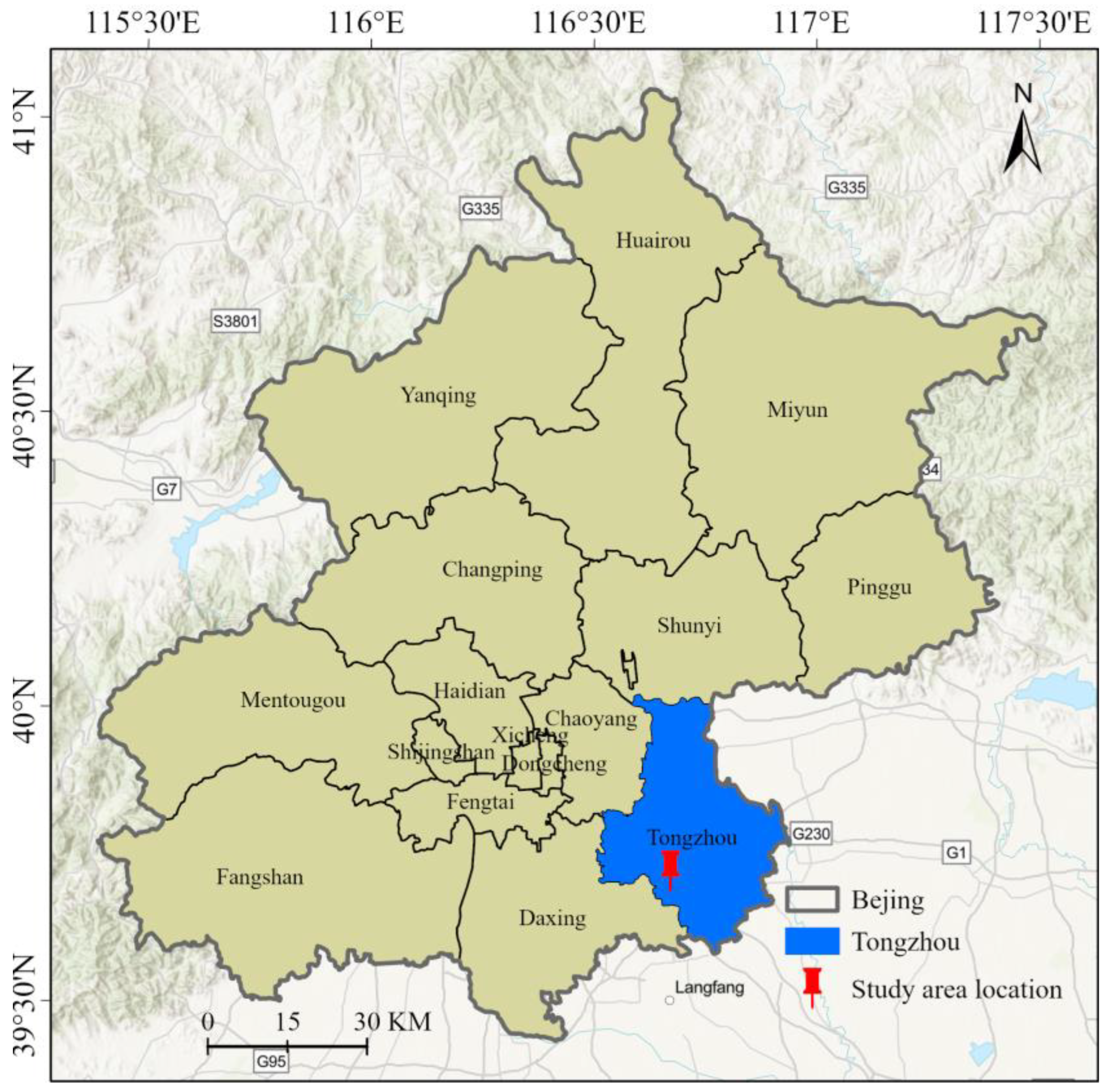
2.1. Study Area

We conducted the field investigation on MNLB on 12–13 August 2023, at the Science and Technology Innovation Demonstration Base of the Beijing Academy of Agriculture and Forestry Sciences in Tongzhou District, Beijing, China (N 116°40′42″, E 39°41′43″) (Figure 1). Tongzhou District features flat terrain with elevations ranging from 8.2 to 27.6 m above sea level. The area experiences a continental monsoon climate, with an average annual temperature of 11.3 °C and an annual precipitation of approximately 620 mm [28]. The study area predominantly contains brown soil, which is highly suitable for crop cultivation. The primary crops grown are wheat and maize. The maize growing season in this region extends from early June to late October. Due to meteorological factors such as rainfall, high humidity, and lower temperatures, MNLB began to manifest in early August and worsened over time.

2.2. Data Acquisition and Processing

2.2.1. Maize Sample Data

In the experimental area, we designed 50 sampling points, each with an area of 1 × 1 m. From these, we obtained 26 healthy samples and 24 samples with early-stage disease. At each site, parameters related to maize leaf physiology, including chlorophyll content, carotenoid content, nitrogen content, and water content, were meticulously quantified. Three maize plants were sampled at each site, and their foliage was promptly transferred to refrigerated containers for swift transport to the laboratory, where comprehensive measurements were undertaken without delay. The quantification of chlorophyll (a + b) and carotenoid content followed the methodology of Lichtenthaler [29]. Total chlorophyll content was derived from the sum of chlorophyll a and b. Leaf nitrogen content was determined using the Kjeldahl method [30]. Leaf water content was determined using the oven-drying technique [31]. Additionally, MNLB severity was assessed at each disease-sampled site. The assessment followed the Ministry of Agriculture’s standard “NY/T 3546-2020: Technical Specification for Diagnosis and Reporting of Maize Northern Leaf Blight” [32]. The disease severity index (DI) depicted MNLB severity. The DI for all samples was below 10%, indicating early disease stages. Figure 2B shows the early symptoms of the disease. Compared to the later stages (Figure 2C), the early symptoms are mainly concentrated on the lower leaves of the maize.

2.2.2. Multiangle Hyperspectral Data

We used the ASD FieldSpec® Pro F spectroradiometer (Analytical Spectral Devices, Boulder, CO, USA) with a multiangle mounting bracket to acquire the multiangle hyperspectral data of the maize. The ASD spectroradiometer covered a spectral range of 350–2500 nm, with a sampling interval of 1.4 nm (350–1000 nm) and 2 nm (1000–2500 nm), and a field of view of 25° [33]. The spectral data were subdivided into 1 nm bandwidths using ASD’s interpolation method. Due to relative humidity, significant noise was observed within the spectral ranges of 1320–1480 nm, 1750–2000 nm, and 2300–2500 nm in the shortwave infrared (SWIR) region. Consequently, these ranges were excluded from subsequent analysis. To ensure compatibility with simulated spectra, the spectral range of 350–399 nm was omitted.
The multiangle bracket is designed to obtain multiangle hyperspectral data (Figure 2A). It securely mounts the fiber optic probe, connected to the ASD spectroradiometer, onto the adjustable upper end of an inverted L-shaped support pole. Controlled by a manual rotational mechanism, it enables the manipulation of the inclined support rod, facilitating diverse viewing angles for data acquisition [26]. We conducted spectral measurements at 13 viewing angles on the solar principal plane, ranging from −60° to +60° at 10° intervals. Here, (−) denotes the backscatter direction (same side as the sun) and (+) denotes the forward scatter direction (opposite side of the sun). The viewing angle is 0° when the view is at nadir [24]. At each angle, we acquired spectral reflectance values from 10 sequences, and their averages were used for analysis. To ensure consistent lighting conditions during spectral acquisition, data for each angle were collected within 30 s, and data for all 13 angles were collected within 7 min. Additionally, canopy spectral reflectance was measured under clear sky conditions between 10:00 AM and 2:00 PM (local Beijing time).

2.3. Feature Extraction and Selection for Early Monitoring of MNLB

2.3.1. Vegetation Indices

VIs, derived from the mathematical transformations of original spectral bands, typically highlight the spectral characteristics of observed targets or mitigate various influences like background and atmospheric effects [34]. Extensive research has demonstrated the effectiveness of VIs in monitoring crop diseases [35]. In this study, we selected 60 VIs related to structural parameters, crop pigments, water content, chlorophyll fluorescence, and crop diseases from the literature as candidate features for constructing the MNLB monitoring model. Table S1 presents the definitions, calculation formulas, and the literature sources for each VI.

2.3.2. Plants Traits Extracted from Hyperspectral Data Based on Hybrid Model

PTs were derived using a hybrid model that combines the PROSAIL model with the Gaussian process regression (GPR) algorithm. Initially, simulated spectra and their corresponding PTs were generated using the PROSAIL model. GPR was then employed to establish the relationship between the simulated spectra and PTs. Building on this framework, a specific retrieval model was developed and applied to real spectral data to estimate PTs [36].
The PROSAIL model integrates the leaf-scale PROSPECT model with the canopy-scale SAIL model [37]. PROSPECT-PRO simulates leaf directional-hemispherical reflectance and transmittance across the optical spectrum from 400 to 2500 nm at a 1 nm spectral resolution. This model includes eight leaf parameters: structure, chlorophyll, carotenoids, anthocyanins, brown pigments, equivalent water thickness, protein content, and carbon-based components [38]. The SAIL model describes the processes of multiple scattering and radiation transfer within the canopy. It considers characteristics such as leaf inclination angle and vertical canopy structure. In our study, we used the 4SAIL model, which incorporates variables such as the leaf area index (LAI), leaf angle distribution, diffuse-to-direct irradiance ratio, hotspot parameter, and solar–target–sensor geometry [39]. Table 1 details the input parameters for the PROSAIL model, meticulously calibrated based on empirical data from our experiment and the relevant literature. Finally, we generated 100,000 simulated spectra and their corresponding PTs using the PROSAIL model.
GPR was selected to couple with PROSAIL to construct a hybrid model for estimating PTs. It is a sophisticated non-parametric statistical method for regression tasks. It uses Gaussian processes to model the distribution over possible functions that fit the data, allowing it to provide both predictions and uncertainty estimates [40]. The key strength of GPR is its flexibility from defining various covariance functions (kernels) that capture different data patterns and structures. This flexibility makes GPR particularly effective in situations where input–output relationships are complex and not easily captured by parametric models [41]. Additionally, GPR’s probabilistic nature provides confidence intervals for predictions, which is valuable in applications requiring an understanding of prediction reliability and uncertainty [42].
We partitioned the 100,000 sets of spectra and PTs generated by PROSAIL into training (70%) and testing (30%) datasets to train and evaluate the GPR model. The performance of the GPR model in retrieving PTs was evaluated using the coefficient of determination (R²), root mean square error (RMSE), and mean absolute error (MAE). We then used the model to estimate PTs from multiangle hyperspectral reflectance data for each sample. Due to limited empirical data, we exclusively validated the performance of Cab and Car retrieval. This approach has proven efficacy in plant disease detection [21,43]. We implemented the hybrid model using the ARTMO toolbox (Automatic Radiative Transfer Model Operator) [44].

2.3.3. Feature Selection for Early Monitoring of MNLB

Our goal was to create a concise and efficient monitoring model. Therefore, we employed multiple feature selection methods to identify the most relevant features for MNLB with minimal redundancy. First, we used a one-way analysis of variance (ANOVA) to evaluate the ability of VIs and PTs to differentiate between healthy and MNLB-infected maize, retaining indicators showing significant differences (p < 0.05). Next, we applied the correlation-based feature selection (CFS) method [45] to further refine the selected features. CFS optimizes feature selection by estimating and ranking the quality of feature subsets through a heuristic approach, ensuring high correlation with the class and minimal inter-feature correlation [46]. The CFS algorithm was implemented in MATLAB. Finally, we conducted a variance inflation factor (VIF) analysis to assess multicollinearity among the features selected by CFS, ensuring the inclusion of the most concise features to enhance model accuracy and efficiency. A VIF value of less than or equal to 10 is generally accepted as indicating minimal multicollinearity among variables [14]. We comprehensively evaluated and selected VIs and PTs obtained from hyperspectral data at various angles.

2.4. Construction and Evaluation of Model for MNLB Early Monitoring

In this research, we used the RF algorithm to construct the model for identifying healthy and early-stage diseased maize. RF is a powerful ensemble learning method widely used for crop disease monitoring [47]. It constructs multiple decision trees during training and outputs the mode of the classes from the individual trees [48]. Each decision tree is built using a random subset of the training data and features, ensuring diversity among the trees. This randomness helps mitigate overfitting and improve generalization performance. Furthermore, RF is robust, scalable, and capable of handling high-dimensional datasets [49]. Hyperparameters in random forests, including the number of trees, random predictors, and maximum depth of trees, are selected by automatic tuning through Bayesian optimization [50].
We developed four crop disease monitoring models using the RF algorithm, leveraging selected VIs and PTs from the hybrid model. These models include the following. (1) VI-based model (VI-RF): this model assesses the efficacy of VIs in monitoring MNLB. (2) Pigment-based model (P-RF): this model evaluates the capability of constructing MNLB monitoring models using only pigment parameters such as Cab, Car, and Anth. (3) PTs-based model (PT-RF): this model incorporates various PTs, including pigments, Cw, Cp, and CBC. (4) Model based on the fusion of PTs and VIs (PTVI-RF): this model integrates PTs and VIs to validate the effectiveness of combining these data types for MNLB monitoring. To assess each model’s accuracy, all 50 samples were used for training and validation via a leave-one-out cross-validation method [51]. Model accuracy was evaluated using OA and the Kappa coefficient (Kappa). The entire process was conducted using MATLAB Statistics and Machine Learning Toolbox.

3. Results

3.1. Evaluation of the Ability of Spectral Feature and Plant Traits for Early Monitoring of MNLB

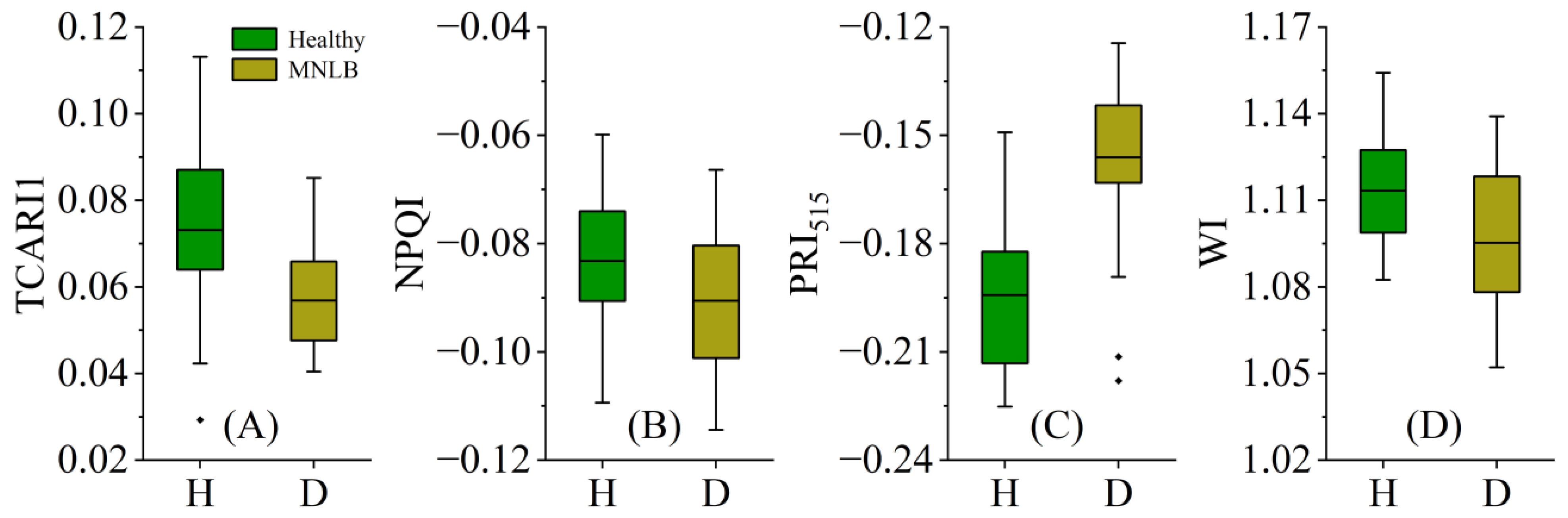
3.1.1. Spectral Reflectance and Vegetation Indices

We assessed the spectral reflectance of healthy and MNLB-affected maize plants, revealing significant differences between the two conditions. Specifically, MNLB-affected maize exhibited significantly lower spectral reflectance than healthy maize in both the visible and near-infrared (NIR) regions. This difference was particularly pronounced within the 510–600 nm and 800–2500 nm ranges (Figure 3A). Moreover, our analysis revealed that the differences in maize spectral reflectance within the visible region were not significant across different observation angles (13 angles from −60° to +60°). However, significant differences were observed in the NIR region. Specifically, spectral reflectance was higher at non-nadir angles compared to the nadir angle (0°) (Figure 3B,C). These distinct spectral variations across different angles offer a promising approach for monitoring MNLB using multiangle hyperspectral data.
Table 2 presents the VIs chosen at each angle that were statistically significant at p < 0.0001 and p < 0.01 levels in distinguishing between healthy and diseased maize samples. This suggests promising potential for these VIs in differentiating between the two sample types. Additionally, the selected VIs varied across different angles. For example, at 0°, four VIs were selected: TCARI1, PRI515, NPQI, and WI. At −10°, only two VIs, TCARI/OSAVI and PRI515, were selected. The study also observed identical VIs across different angles, suggesting robust generalization. For instance, PRI515 was selected at eight angles, WI at seven angles, and NPQI at six angles. The VIF test (Table S2) indicated that the VIFs of the selected VIs at each angle were all below five, suggesting minimal to nonexistent covariance between the VIs. This makes them suitable for constructing disease monitoring models. Figure 4 illustrates the distinctions between healthy and diseased samples based on the four selected VIs at 0°. These VIs exhibited significant differences between the two sample types, with a noticeable downward trend in TCARI1, NPQI, and WI for diseased samples compared to healthy ones, and an upward trend in PRI.

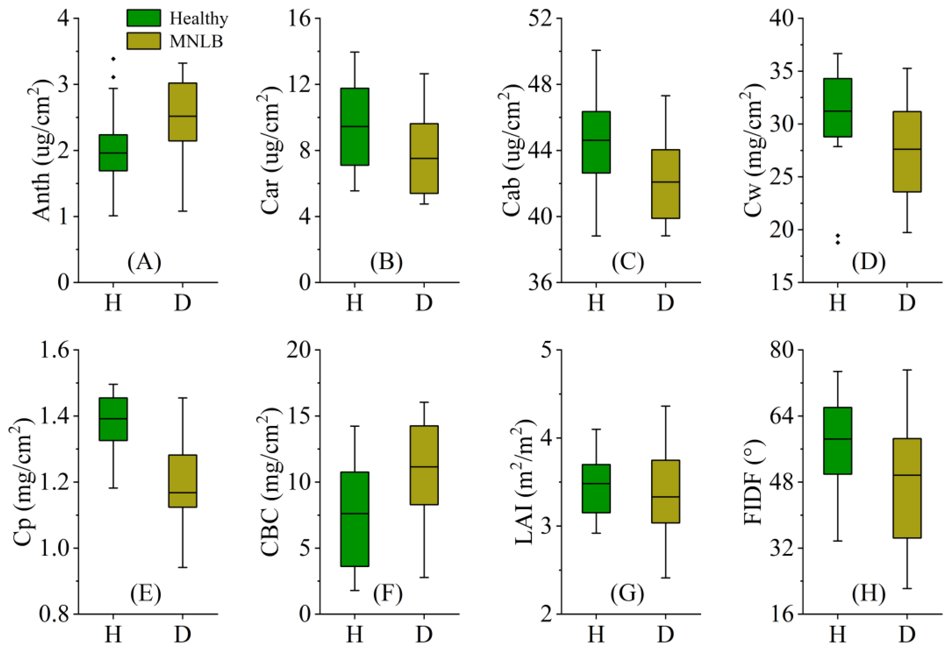
3.1.2. PTs Obtained from the Inversion of the Hybrid Model

Inverting PTs using hybrid models yielded favorable outcomes (Tables S3–S5). Most PTs inversion accuracies had R2 values over 0.9, except for Cp and LIDF, which had accuracies in the 0.8 to 0.9 range. Field data validation confirmed the satisfactory accuracies of Car and Cab, with R2 values of 0.52 and 0.65, and RMSE values of 6.36 for Car and 0.97 for Cab (Figure S1). Additionally, model accuracy for each PT showed minimal variation across different angles. For instance, R² for Cab ranged from 0.94 to 0.96, with RMSE values of 3.31 to 4.10 across 13 angles from −60° to +60°. The minimal variation in model accuracy across different angles may result from the data used to construct the model being generated by PROSAIL simulations, which are less affected by external factors. ANOVA test results of inverted parameters.
ANOVA test results for the inverted PTs (Table 3) showed that most PTs (Cab, Car, Anth, Cw, Cp, and CBC) obtained by inversion at different angles exhibited significance differences between diseased and healthy samples (p < 0.05). However, for a few PTs (Cab, Cw, and Cp) obtained at angles from 40° to 60°, the differences were not statistically significant (p > 0.05). Many structural parameters (LAI and LIDF) obtained at different angles did not pass the ANOVA test, indicating non-significant differences. Consequently, these structural parameters were excluded from the disease model construction. Furthermore, most PTs at each angle passed the VIF test (VIF < 10), as indicated in Table S6.
Figure 5 illustrates the variability between healthy and diseased samples for PTs obtained by inversion at 0°. Significant differences were observed in all PTs except LAI. Notably, Car and CBC exhibited an increasing trend, while Cab, Anth, Cw, Cp, and FIDA showed a decreasing trend in diseased samples compared to healthy ones. Similarly, in Figure 6 plots the differences in measured PTs (Cab, Car, LNC, and LWC) between diseased and healthy samples. All these PTs were significantly different between the two sample types, with values lower in diseased samples than in healthy samples. These findings provide a foundation for constructing a monitoring model based on PTs.

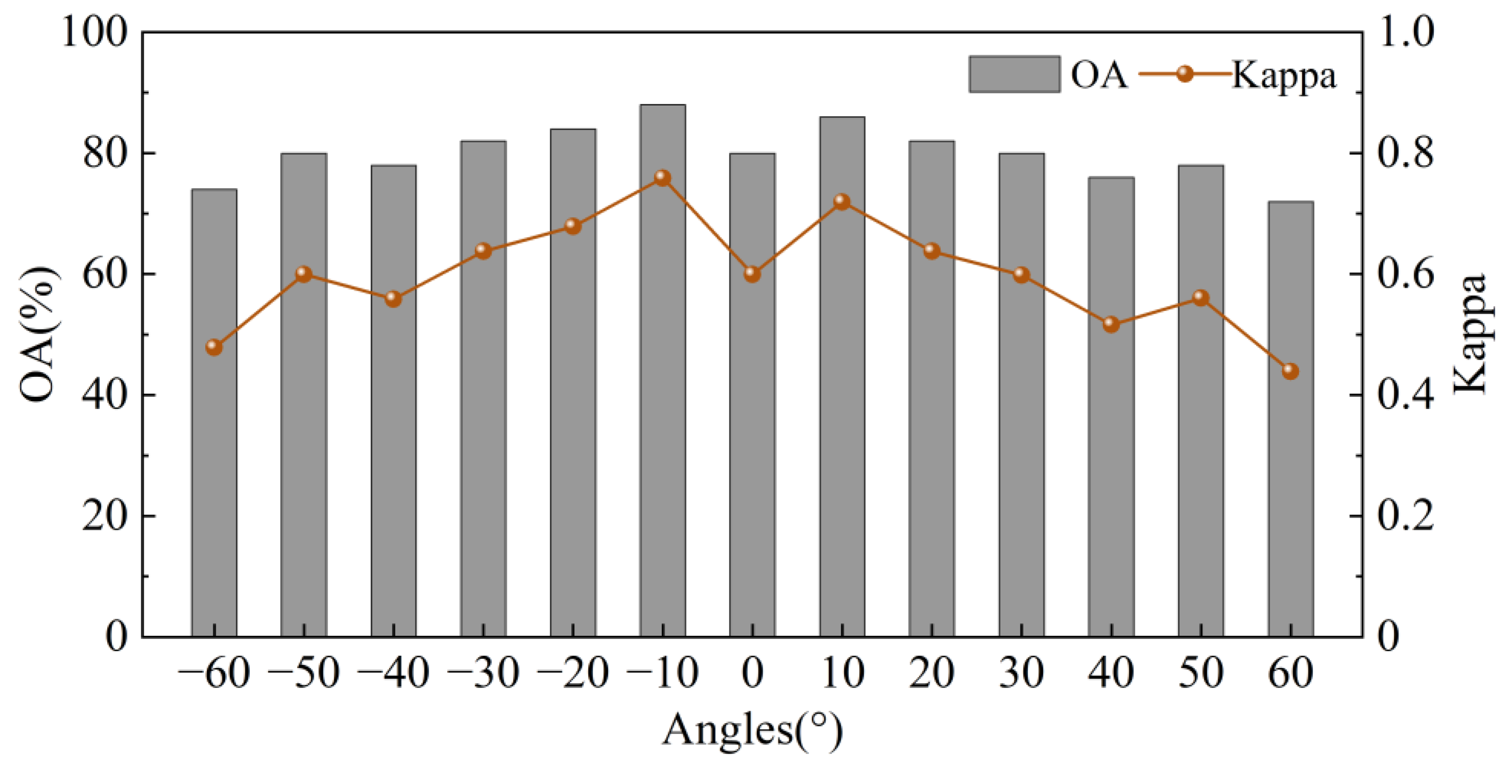
3.2. Performance Evaluation of the MNLB Early Monitoring Model Based on Various Features Using Multiangle Hyperspectral Data

Table 4 shows the outcomes of four distinct disease monitoring models developed using data from 13 angles. The results indicate that the P-RF model consistently had lower accuracy compared to the other models. In contrast, the PT-RF model, which incorporates crop pigmentation along with parameters such as Cw, Cp, and CBC, exhibited notable improvements in accuracy. For example, at 0°, the OA and Kappa for the P-RF model were 60% and 0.20, respectively. In contrast, the PT-RF model had values of 74% and 0.48. These findings suggest that MNLB can be effectively monitored using inverted PTs alone. Furthermore, the VI-RF model exhibited greater accuracy than the P-RF model, with performance levels closely resembling those of the PT-RF model. For instance, at 0°, the OA and Kappa of the VI-RF model were 76% and 0.52, slightly surpassing the PT-RF model’s values of 74% and 0.48. Similarly, at −40°, both models achieved an OA of 76% and a Kappa of 0.52. The PTVI-RF model showed the highest accuracy among the four models, consistently outperforming the VI-RF and PT-RF models across all 13 angles. For example, at 0°, the OA of the PTVI-RF model was 4% and 6% higher compared to the former two models. Similarly, at −10°, the PTVI-RF model was 8% and 6% higher, respectively. These results suggest that models integrating VIs with PTs offer greater advantages compared to models using a single VI or PTs alone.
The results show that angles significantly impact model accuracy (Figure 7). Specifically, the model’s accuracy at smaller off-nadir angles (±10° to ±30°) is higher than that at nadir (0°), especially at ±10°. For example, the PTVI-RF model’s OA at 0° is 80% with a Kappa of 0.60. At −10°, the OA increased to 88% and Kappa increased to 0.76, which were the highest accuracies obtained. At 10°, the accuracy is slightly lower than at −10°, with an OA of 86% and a Kappa of 0.72. Notably, the model performs worse at larger off-nadir angles (±40° to ±60°) compared to 0°. For example, the OA of VPWN-RF at −60° and 60° is only 74% and 72%, with Kappa values of 0.48 and 0.44, respectively. Overall, using hyperspectral data acquired at smaller off-nadir angles can effectively improve MNLB monitoring accuracy.

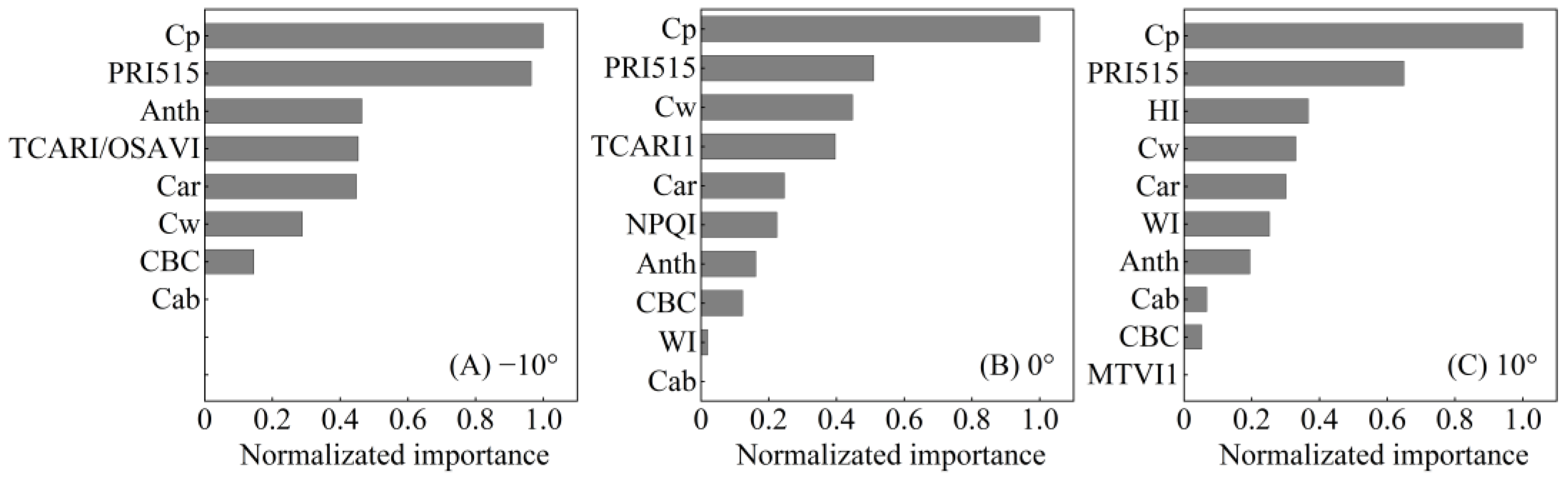
3.3. Contribution of VIs and PTs in the MNLB Early Monitoring Model

The contribution of optimal VIs and PTs for monitoring MNLB was evaluated. Feature importance in the PTVI-RF model at −10°, 0°, and 10° was ranked using the out-of-bag (OOB) method in RF classification. All feature importance scores normalized for comparison. Model feature importance was presented at these three angles because the model achieves the best accuracy at −10° and 10°, while 0° is commonly used. Figure 8 shows the ranking of feature importance in the VPWN-RF model across the three angles. Overall, the contributions of VIs and PTs varied across angles. However, Cp and PRI515 consistently ranked highest in importance across all three angles, indicating their significant contribution to the model for monitoring MNLB. Additionally, Cw ranked third at 0° and fourth at 10°. CBC and Cab exhibited lower contributions across all angles. Except for PRI515, the contribution of VIs was generally moderate.

4. Discussion

4.1. VIs and PTs for Early Monitoring of MNLB

This study demonstrated the effectiveness of VIs and PTs extracted from hyperspectral data in monitoring MNLB. Optimal VIs and PTs for constructing a disease monitoring model were identified through feature selection. Several selected VIs recurred at different angles and showed significant differences between healthy and diseased samples, indicating their potential for monitoring MNLB. For example, PRI515 appeared at eight angles, WI at seven angles, and NPQI at six angles. Studies have shown that PRI correlates with leaf light use efficiency (LUE) and serves as an indicator for monitoring plant stress [52]. Changes in PRI during disease development may reflect reduced assimilation and stomatal conductance [53]. Similarly, NPQI is associated with chlorophyll degradation. Disease-induced cellular damage in leaves leads to decreased chlorophyll content, which in turn leads to a decrease in NPQI, consistent with the findings of Zarco-Tejada et al. [20]. WI indicates water content in plant leaves. Disease stress causes water loss, leading to a lower WI in diseased plants compared to healthy plants [15].
Regarding PTs, the study showed decreases in Car, Cab, Cw, and Cp, and increases in CBC and Anth in diseased maize compared to healthy maize. These changes are related to physiological processes in the leaves. The MNLB pathogen infects maize leaves, destroying the cellular structure, which results in decreased levels of Car, Cab, and Cw. The decrease in Cp may be due to pathogen infestation altering leaf nitrogen metabolism, including glutamine synthetase and xylem nitrogen compound accumulation [54]. Disease infestation enhances Anth synthesis in response to oxidative stress [55]. In conclusion, the selected PTs and VIs showed significant differences between healthy and diseased maize plants, contributing to the development of robust models for monitoring MNLB.

4.2. The Model for Early Monitoring MNLB

This study developed four models for monitoring MNLB (VI-RF, P-RF, PT-RF, and PTVI-RF). The results revealed that when the P-RF model relied solely on pigments (Car, Cab, and Anth), its accuracy was consistently suboptimal across all angles, with OA below 70% for all angles except ±10° and ±20°. The PT-RF model, incorporating Cp, Cw, and pigments, showed varying degrees of improvement across all angles compared to the P-RF model. Specifically, OA surpassed 70% for all angles except at 40°, 50°, and 60°, achieving 82% at −10° and 84% at 10°. These findings suggest that PTs like Cp and Cw play a crucial role in the model, effectively enhancing disease characterization. This is further supported by feature importance analysis, where Cp consistently ranked as the most important feature at angles of −10°, 0°, and 10°, while Cw also maintained a prominent position. These findings align with those reported by Camino et al. [56].
Models constructed solely with VIs (VI-RF) did not achieve the highest accuracy, possibly due to their reliance on a few spectral bands containing limited information. Additionally, these VIs may not fully account for the impact of canopy heterogeneity on the spectrum. The PTVI-RF model, which combines VIs with PTs, demonstrated the best performance among the four models, highlighting the effectiveness of integrating both data types in improving disease monitoring accuracy. For instance, at −20°, the PTVI-RF model enhanced OA by 4% and 6% compared to the VI-RF and PT-RF models, respectively. Similar findings have been reported in prior studies [21]. The superior performance of the PTVI-RF model can be attributed to the synergistic effect of VIs and PTs, enhancing the model’s ability to reflect MNLB. This integration enables the model to capture information on disease-induced changes in internal leaf parameters and insights into disease-induced spectral alterations. The data used to construct the MNLB early monitoring model were collected from a single location, which may affect the model’s generalizability. In the future, we will collect data from multiple location to construct and validate the model, thereby improving its generalizability. Due to the small sample size obtained from the experiment, the leave-one-out cross-validation method was used during the construction of the model. This method may not fully validate the model’s generalizability. In the future, we will obtain more independent data from different locations to validate the model.

4.3. The Impact of Angles on the Early Monitoring Model of MNLB

The narrow range of single observation angles limits MNLB early monitoring. Observing from multiple angles allows acquiring information on both the lower and middle layers of the crop, offering significant potential for monitoring early MNLB in the lower part of the maize canopy. This study investigates the performance of the MNLB monitoring model with multiangle hyperspectral data (−60° to 60°). The results show that models at smaller off-nadir angles (±10° to ±30°) have higher accuracies than those at nadir (0°). In contrast, model accuracies at larger angles (±40° to ±60°) did not exceed those at 0°. The suitability of small angle ranges, especially −10° and 10°, for monitoring early MNLB may be attributed to two primary reasons. First, it may be related to the pathogenic characteristics of MNLB. MNLB is a bottom-up disease, meaning it primarily infects the lower leaves of the maize canopy in the early stages. Second, the small field of view angle corresponds to the middle and lower parts of the crop canopy, allowing for more information about the disease in the lower part of the crop to be obtained. In contrast, a larger field of view range corresponds to the upper–middle part of the crop canopy, making it difficult to obtain information on MNLB in the lower part of the maize [27]. This assertion is supported by the findings of He et al. [22], who used multiangle hyperspectral data to monitor wheat powdery mildew, a disease also characterized by bottom-up progression, and found that a small angle range (10° to 30°) was most suitable for disease monitoring.
In the future, we will collect data on diseases of varying severity and construct a monitoring model that covers the entire process of disease development, from mild to severe. Additionally, the MNLB monitoring method based on ground-based multi-angle hyperspectral data will be applied to UAV hyperspectral platforms to enhance the utility of the disease monitoring model. We will focus on verifying whether the optimal angles determined from ground data provide the best performance in UAV data. Furthermore, the effectiveness of the MNLB early monitoring method will be evaluated for various diseases that occur early in the lower part of the crop canopy, such as wheat powdery mildew, to confirm its applicability in different agricultural environments. This study focuses on monitoring milder symptoms in the early stages of MNLB.

5. Conclusions

This study evaluates the effectiveness of combined VIs and PTs derived from multiangle hyperspectral data for early monitoring MNLB. Our results showed that VIs and PTs extracted from hyperspectral data and subjected to feature selection analysis were able to effectively differentiate between healthy and early diseased maize plants. The VPWN-RF model, integrating VIs and PTs, outperformed models based solely on VIs or PTs. Feature importance analysis consistently ranked Cp and PIR515 highest, highlighting their significant contributions to early MNLB monitoring. Our results also emphasize the significant impact of viewing angle on MNLB monitoring accuracy. We found that smaller off-nadir angles (±10° to ±30°) yielded higher accuracy than nadir angles (0°), whereas larger off-nadir angles (±40° to ±60°) reduced accuracy. Notably, VPWN-RF achieved the highest accuracy at −10° with an OA of 88% and a Kappa of 0.76, owing to its capability to capture information from the lower crop canopy at small viewing angles. In summary, we proposed a model (PTVI-RF) that combines PTs and VIs extracted from multiangle hyperspectral data using the RF algorithm, effectively improving the early monitoring accuracy of MNLB. It offers valuable insights for early disease monitoring in lower crop canopies, enabling timely interventions by crop managers to mitigate potential losses.

Supplementary Materials

The following supporting information can be downloaded at: https://www.mdpi.com/article/10.3390/agriculture14081311/s1. Table S1. Candidate VIs used for MNLB monitoring model construction. Table S2. Results of variance inflation factor (VIF) test for selected VIs. Table S3. R2 of the accuracy of the hybrid model for retrieving plant traits. Table S4. RMSE of the accuracy of the hybrid model for retrieving plant traits. Table S5. MEA of the accuracy of the hybrid model for retrieving plant traits. Table S6. Results of variance inflation factor (VIF) test for plant traits. Figure S1. Results of validation of PTs (Car and Cab) based on hybrid model using field-acquired data. A and B are Cab and Car, respectively [57,58,59,60,61,62,63,64,65,66,67,68,69,70,71,72,73,74,75,76,77,78,79,80,81,82].

Author Contributions

Conceptualization, A.G. and W.H.; methodology, A.G. and K.W.; software, A.G. and X.C.; formal analysis, B.Q.; investigation, A.G., B.Q. and X.C.; writing—original draft, A.G.; writing—review and editing, A.G., K.W. and W.H.; supervision, W.H.; funding acquisition, K.W. and W.H. All authors have read and agreed to the published version of the manuscript.

Funding

This research was funded by the National Key Research and Development Program (No. 2023YFD2000104) and the National Natural Science Foundation of China (No. 42201365).

Institutional Review Board Statement

Not applicable.

Data Availability Statement

The data are available from the authors upon reasonable request.

Acknowledgments

We thank the researchers at the Science and Technology Innovation Demonstration Base of Beijing Academy of Agriculture and Forestry Sciences for their help in obtaining the experimental data.

Conflicts of Interest

The authors declare no conflicts of interest.

References

  1. Luo, P.; Ye, H.; Huang, W.; Liao, J.; Jiao, Q.; Guo, A.; Qian, B. Enabling Deep-Neural-Network-Integrated Optical and SAR Data to Estimate the Maize Leaf Area Index and Biomass with Limited In Situ Data. Remote Sens. 2022, 14, 5624. [Google Scholar] [CrossRef]
  2. Resti, Y.; Irsan, C.; Putri, M.T.; Yani, I.; Ansyori, A.; Suprihatin, B. Identification of corn plant diseases and pests based on digital images using multinomial naïve bayes and k-nearest neighbor. Sci. Technol. Indones. 2022, 7, 29–35. [Google Scholar] [CrossRef]
  3. DeChant, C.; Wiesner-Hanks, T.; Chen, S.; Stewart, E.L.; Yosinski, J.; Gore, M.A.; Nelson, R.J.; Lipson, H. Automated identification of northern leaf blight-infected maize plants from field imagery using deep learning. Phytopathology 2017, 107, 1426–1432. [Google Scholar] [CrossRef] [PubMed]
  4. Rai, C.K.; Pahuja, R. Northern maize leaf blight disease detection and segmentation using deep convolution neural networks. Multimed. Tools Appl. 2024, 83, 19415–19432. [Google Scholar] [CrossRef]
  5. Stewart, E.L.; Wiesner-Hanks, T.; Kaczmar, N.; DeChant, C.; Wu, H.; Lipson, H.; Nelson, R.J.; Gore, M.A. Quantitative phenotyping of northern leaf blight in UAV images using deep learning. Remote Sens. 2019, 11, 2209. [Google Scholar] [CrossRef]
  6. Grisham, M.P.; Johnson, R.M.; Zimba, P.V. Detecting Sugarcane yellow leaf virus infection in asymptomatic leaves with hyperspectral remote sensing and associated leaf pigment changes. J. Virol. Methods 2010, 167, 140–145. [Google Scholar] [CrossRef] [PubMed]
  7. Zhou, R.-Q.; Jin, J.-J.; Li, Q.-M.; Su, Z.-Z.; Yu, X.-J.; Tang, Y.; Luo, S.-M.; He, Y.; Li, X.-L. Early Detection of Magnaporthe oryzae-Infected Barley Leaves and Lesion Visualization Based on Hyperspectral Imaging. Front. Plant Sci. 2019, 9, 1962. [Google Scholar] [CrossRef]
  8. Gao, Z.; Khot, L.R.; Naidu, R.A.; Zhang, Q. Early detection of grapevine leafroll disease in a red-berried wine grape cultivar using hyperspectral imaging. Comput. Electron. Agric. 2020, 179, 105807. [Google Scholar] [CrossRef]
  9. Mahlein, A.K.; Kuska, M.T.; Behmann, J.; Polder, G.; Walter, A. Hyperspectral Sensors and Imaging Technologies in Phytopathology: State of the Art. Annu. Rev. Phytopathol. 2018, 56, 535–558. [Google Scholar] [CrossRef]
  10. Khan, I.H.; Liu, H.; Li, W.; Cao, A.; Wang, X.; Liu, H.; Cheng, T.; Tian, Y.; Zhu, Y.; Cao, W. Early detection of powdery mildew disease and accurate quantification of its severity using hyperspectral images in wheat. Remote Sens. 2021, 13, 3612. [Google Scholar] [CrossRef]
  11. Rumpf, T.; Mahlein, A.-K.; Steiner, U.; Oerke, E.-C.; Dehne, H.-W.; Plümer, L. Early detection and classification of plant diseases with support vector machines based on hyperspectral reflectance. Comput. Electron. Agric. 2010, 74, 91–99. [Google Scholar] [CrossRef]
  12. Cheng, T.; Rivard, B.; Sánchez-Azofeifa, A.G.; Féret, J.-B.; Jacquemoud, S.; Ustin, S.L. Deriving leaf mass per area (LMA) from foliar reflectance across a variety of plant species using continuous wavelet analysis. ISPRS-J. Photogramm. Remote Sens. 2014, 87, 28–38. [Google Scholar] [CrossRef]
  13. Lin, D.; Li, G.; Zhu, Y.; Liu, H.; Li, L.; Fahad, S.; Zhang, X.; Wei, C.; Jiao, Q. Predicting copper content in chicory leaves using hyperspectral data with continuous wavelet transforms and partial least squares. Comput. Electron. Agric. 2021, 187, 106293. [Google Scholar] [CrossRef]
  14. Tian, L.; Xue, B.; Wang, Z.; Li, D.; Yao, X.; Cao, Q.; Zhu, Y.; Cao, W.; Cheng, T. Spectroscopic detection of rice leaf blast infection from asymptomatic to mild stages with integrated machine learning and feature selection. Remote Sens. Environ. 2021, 257, 112350. [Google Scholar] [CrossRef]
  15. Hornero, A.; Hernández-Clemente, R.; North, P.R.; Beck, P.; Boscia, D.; Navas-Cortes, J.A.; Zarco-Tejada, P.J. Monitoring the incidence of Xylella fastidiosa infection in olive orchards using ground-based evaluations, airborne imaging spectroscopy and Sentinel-2 time series through 3-D radiative transfer modelling. Remote Sens. Environ. 2020, 236, 111480. [Google Scholar] [CrossRef]
  16. Yao, Z.; Lei, Y.; He, D. Early Visual Detection of Wheat Stripe Rust Using Visible/Near-Infrared Hyperspectral Imaging. Sensors 2019, 19, 952. [Google Scholar] [CrossRef]
  17. Cheng, X.; Huang, M.; Guo, A.; Huang, W.; Cai, Z.; Dong, Y.; Guo, J.; Hao, Z.; Huang, Y.; Ren, K. Early Detection of Rubber Tree Powdery Mildew by Combining Spectral and Physicochemical Parameter Features. Remote Sens. 2024, 16, 1634. [Google Scholar] [CrossRef]
  18. Watt, M.S.; Poblete, T.; de Silva, D.; Estarija, H.J.C.; Hartley, R.J.; Leonardo, E.M.C.; Massam, P.; Buddenbaum, H.; Zarco-Tejada, P.J. Prediction of the severity of Dothistroma needle blight in radiata pine using plant based traits and narrow band indices derived from UAV hyperspectral imagery. Agric. For. Meteorol. 2023, 330, 109294. [Google Scholar] [CrossRef]
  19. Zarco-Tejada, P.J.; Camino, C.; Beck, P.S.A.; Calderon, R.; Hornero, A.; Hernández-Clemente, R.; Kattenborn, T.; Montes-Borrego, M.; Susca, L.; Morelli, M.; et al. Previsual symptoms of Xylella fastidiosa infection revealed in spectral plant-trait alterations. Nat. Plants 2018, 4, 432–439. [Google Scholar] [CrossRef]
  20. Zarco-Tejada, P.; Poblete, T.; Camino, C.; Gonzalez-Dugo, V.; Calderon, R.; Hornero, A.; Hernandez-Clemente, R.; Román-Écija, M.; Velasco-Amo, M.; Landa, B. Divergent abiotic spectral pathways unravel pathogen stress signals across species. Nat. Commun. 2021, 12, 6088. [Google Scholar] [CrossRef]
  21. Poblete, T.; Navas-Cortes, J.; Camino, C.; Calderon, R.; Hornero, A.; Gonzalez-Dugo, V.; Landa, B.; Zarco-Tejada, P. Discriminating Xylella fastidiosa from Verticillium dahliae infections in olive trees using thermal-and hyperspectral-based plant traits. ISPRS-J. Photogramm. Remote Sens. 2021, 179, 133–144. [Google Scholar] [CrossRef]
  22. He, L.; Qi, S.-L.; Duan, J.-Z.; Guo, T.-C.; Feng, W.; He, D.-X. Monitoring of Wheat powdery mildew disease severity using multiangle hyperspectral remote sensing. IEEE Trans. Geosci. Remote Sens. 2020, 59, 979–990. [Google Scholar] [CrossRef]
  23. Wang, L.; Dong, T.; Zhang, G.; Niu, Z. LAI retrieval using PROSAIL model and optimal angle combination of multi-angular data in wheat. IEEE J. Sel. Top. Appl. Earth Obs. Remote Sens. 2013, 6, 1730–1736. [Google Scholar] [CrossRef]
  24. He, L.; Song, X.; Feng, W.; Guo, B.-B.; Zhang, Y.-S.; Wang, Y.-H.; Wang, C.-Y.; Guo, T.-C. Improved remote sensing of leaf nitrogen concentration in winter wheat using multi-angular hyperspectral data. Remote Sens. Environ. 2016, 174, 122–133. [Google Scholar] [CrossRef]
  25. He, L.; Zhang, H.-Y.; Zhang, Y.-S.; Song, X.; Feng, W.; Kang, G.-Z.; Wang, C.-Y.; Guo, T.-C. Estimating canopy leaf nitrogen concentration in winter wheat based on multi-angular hyperspectral remote sensing. Eur. J. Agron. 2016, 73, 170–185. [Google Scholar] [CrossRef]
  26. Wu, B.; Ye, H.; Huang, W.; Wang, H.; Luo, P.; Ren, Y.; Kong, W. Monitoring the Vertical Distribution of Maize Canopy Chlorophyll Content Based on Multi-Angular Spectral Data. Remote Sens. 2021, 13, 987. [Google Scholar] [CrossRef]
  27. Song, L.; Wang, L.; Yang, Z.; He, L.; Feng, Z.; Duan, J.; Feng, W.; Guo, T. Comparison of algorithms for monitoring wheat powdery mildew using multi-angular remote sensing data. Crop J. 2022, 10, 1312–1322. [Google Scholar] [CrossRef]
  28. Wang, Y.; Xu, X.; Huang, L.; Yang, G.; Fan, L.; Wei, P.; Chen, G. An improved CASA model for estimating winter wheat yield from remote sensing images. Remote Sens. 2019, 11, 1088. [Google Scholar] [CrossRef]
  29. Lichtenthaler, H.K. Chlorophylls and carotenoids: Pigments of photosynthetic biomembranes. Methods Enzymol. 1987, 148, 350–382. [Google Scholar]
  30. Kjeldahl, J. Neue Methode zur Bestimmung des Stickstoffs in organischen Körpern. Z. Anal. Chem. 1883, 22, 366–382. [Google Scholar] [CrossRef]
  31. Cheng, T.; Rivard, B.; Sanchez-Azofeifa, A. Spectroscopic determination of leaf water content using continuous wavelet analysis. Remote Sens. Environ. 2011, 115, 659–670. [Google Scholar] [CrossRef]
  32. Wu, Q.; Zeng, J.; Wu, K. Research and application of crop pest monitoring and early warning technology in China. Front. Agric. Sci. Eng. 2022, 9, 19–36. [Google Scholar] [CrossRef]
  33. Tian, L.; Wang, Z.; Xue, B.; Li, D.; Zheng, H.; Yao, X.; Zhu, Y.; Cao, W.; Cheng, T. A disease-specific spectral index tracks Magnaporthe oryzae infection in paddy rice from ground to space. Remote Sens. Environ. 2023, 285, 113384. [Google Scholar] [CrossRef]
  34. Zhang, J.; Huang, Y.; Pu, R.; Gonzalez-Moreno, P.; Yuan, L.; Wu, K.; Huang, W. Monitoring plant diseases and pests through remote sensing technology: A review. Comput. Electron. Agric. 2019, 165, 104943. [Google Scholar] [CrossRef]
  35. Mahlein, A.-K.; Rumpf, T.; Welke, P.; Dehne, H.-W.; Plümer, L.; Steiner, U.; Oerke, E.-C. Development of spectral indices for detecting and identifying plant diseases. Remote Sens. Environ. 2013, 128, 21–30. [Google Scholar] [CrossRef]
  36. Tagliabue, G.; Boschetti, M.; Bramati, G.; Candiani, G.; Colombo, R.; Nutini, F.; Pompilio, L.; Rivera-Caicedo, J.P.; Rossi, M.; Rossini, M. Hybrid retrieval of crop traits from multi-temporal PRISMA hyperspectral imagery. ISPRS-J. Photogramm. Remote Sens. 2022, 187, 362–377. [Google Scholar] [CrossRef] [PubMed]
  37. Verhoef, W.; Jia, L.; Xiao, Q.; Su, Z. Unified optical-thermal four-stream radiative transfer theory for homogeneous vegetation canopies. IEEE Trans. Geosci. Remote Sens. 2007, 45, 1808–1822. [Google Scholar] [CrossRef]
  38. Chakhvashvili, E.; Siegmann, B.; Muller, O.; Verrelst, J.; Bendig, J.; Kraska, T.; Rascher, U. Retrieval of Crop Variables from Proximal Multispectral UAV Image Data Using PROSAIL in Maize Canopy. Remote Sens. 2022, 14, 1247. [Google Scholar] [CrossRef] [PubMed]
  39. Sinha, S.K.; Padalia, H.; Dasgupta, A.; Verrelst, J.; Rivera, J.P. Estimation of leaf area index using PROSAIL based LUT inversion, MLRA-GPR and empirical models: Case study of tropical deciduous forest plantation, North India. Int. J. Appl. Earth Obs. Geoinf. 2020, 86, 102027. [Google Scholar] [CrossRef]
  40. Adeluyi, O.; Harris, A.; Verrelst, J.; Foster, T.; Clay, G.D. Estimating the phenological dynamics of irrigated rice leaf area index using the combination of PROSAIL and Gaussian Process Regression. Int. J. Appl. Earth Obs. Geoinf. 2021, 102, 102454. [Google Scholar] [CrossRef]
  41. Danner, M.; Berger, K.; Wocher, M.; Mauser, W.; Hank, T. Efficient RTM-based training of machine learning regression algorithms to quantify biophysical & biochemical traits of agricultural crops. ISPRS-J. Photogramm. Remote Sens. 2021, 173, 278–296. [Google Scholar]
  42. Estévez, J.; Salinero-Delgado, M.; Berger, K.; Pipia, L.; Rivera-Caicedo, J.P.; Wocher, M.; Reyes-Muñoz, P.; Tagliabue, G.; Boschetti, M.; Verrelst, J. Gaussian processes retrieval of crop traits in Google Earth Engine based on Sentinel-2 top-of-atmosphere data. Remote Sens. Environ. 2022, 273, 112958. [Google Scholar] [CrossRef] [PubMed]
  43. Poblete, T.; Camino, C.; Beck, P.; Hornero, A.; Kattenborn, T.; Saponari, M.; Boscia, D.; Navas-Cortes, J.A.; Zarco-Tejada, P.J. Detection of Xylella fastidiosa infection symptoms with airborne multispectral and thermal imagery: Assessing bandset reduction performance from hyperspectral analysis. ISPRS-J. Photogramm. Remote Sens. 2020, 162, 27–40. [Google Scholar] [CrossRef]
  44. Verrelst, J.; Rivera, J.P.; Veroustraete, F.; Muñoz-Marí, J.; Clevers, J.G.; Camps-Valls, G.; Moreno, J. Experimental Sentinel-2 LAI estimation using parametric, non-parametric and physical retrieval methods–A comparison. ISPRS-J. Photogramm. Remote Sens. 2015, 108, 260–272. [Google Scholar] [CrossRef]
  45. Chuanlei, Z.; Shanwen, Z.; Jucheng, Y.; Yancui, S.; Jia, C. Apple leaf disease identification using genetic algorithm and correlation based feature selection method. Int. J. Agric. Biol. Eng. 2017, 10, 74–83. [Google Scholar]
  46. Hall, M.A. Correlation-Based Feature Selection for Machine Learning; The University of Waikato: Hamilton, New Zealand, 1999. [Google Scholar]
  47. Berger, K.; Machwitz, M.; Kycko, M.; Kefauver, S.C.; Van Wittenberghe, S.; Gerhards, M.; Verrelst, J.; Atzberger, C.; van der Tol, C.; Damm, A. Multi-sensor spectral synergies for crop stress detection and monitoring in the optical domain: A review. Remote Sens. Environ. 2022, 280, 113198. [Google Scholar] [CrossRef]
  48. Breiman, L. Random forests. Mach. Learn. 2001, 45, 5–32. [Google Scholar] [CrossRef]
  49. Behmann, J.; Steinrücken, J.; Plümer, L. Detection of early plant stress responses in hyperspectral images. ISPRS-J. Photogramm. Remote Sens. 2014, 93, 98–111. [Google Scholar] [CrossRef]
  50. Su, J.; Liu, C.; Coombes, M.; Hu, X.; Wang, C.; Xu, X.; Li, Q.; Guo, L.; Chen, W.-H. Wheat yellow rust monitoring by learning from multispectral UAV aerial imagery. Comput. Electron. Agric. 2018, 155, 157–166. [Google Scholar] [CrossRef]
  51. Zhen, J.; Jiang, X.; Xu, Y.; Miao, J.; Zhao, D.; Wang, J.; Wang, J.; Wu, G. Mapping leaf chlorophyll content of mangrove forests with Sentinel-2 images of four periods. Int. J. Appl. Earth Obs. Geoinf. 2021, 102, 102387. [Google Scholar] [CrossRef]
  52. Zarco-Tejada, P.J.; Berni, J.A.; Suárez, L.; Sepulcre-Cantó, G.; Morales, F.; Miller, J.R. Imaging chlorophyll fluorescence with an airborne narrow-band multispectral camera for vegetation stress detection. Remote Sens. Environ. 2009, 113, 1262–1275. [Google Scholar] [CrossRef]
  53. López-López, M.; Calderón, R.; González-Dugo, V.; Zarco-Tejada, P.J.; Fereres, E. Early detection and quantification of almond red leaf blotch using high-resolution hyperspectral and thermal imagery. Remote Sens. 2016, 8, 276. [Google Scholar] [CrossRef]
  54. Purcino, R.P.; Medina, C.L.; de Souza, D.M.; Winck, F.V.; Machado, E.C.; Novello, J.C.; Machado, M.A.; Mazzafera, P. Xylella fastidiosa disturbs nitrogen metabolism and causes a stress response in sweet orange Citrus sinensis cv. Pera. J. Exp. Bot. 2007, 58, 2733–2744. [Google Scholar] [CrossRef]
  55. Suarez, L.; Zhang, P.; Sun, J.; Wang, Y.; Poblete, T.; Hornero, A.; Zarco-Tejada, P.J. Assessing wine grape quality parameters using plant traits derived from physical model inversion of hyperspectral imagery. Agric. For. Meteorol. 2021, 306, 108445. [Google Scholar] [CrossRef]
  56. Camino, C.; Calderón, R.; Parnell, S.; Dierkes, H.; Chemin, Y.; Román-Écija, M.; Montes-Borrego, M.; Landa, B.B.; Navas-Cortes, J.A.; Zarco-Tejada, P.J.; et al. Detection of Xylella fastidiosa in almond orchards by synergic use of an epidemic spread model and remotely sensed plant traits. Remote Sens. Environ. 2021, 260, 112420. [Google Scholar] [CrossRef] [PubMed]
  57. Hunt, E.R., Jr.; Daughtry, C.S.; Eitel, J.U.; Long, D.S. Remote sensing leaf chlorophyll content using a visible band index. Agron. J. 2011, 103, 1090–1099. [Google Scholar] [CrossRef]
  58. Jurgens, C. The modified normalized difference vegetation index (mNDVI) a new index to determine frost damages in agriculture based on Landsat TM data. Int. J. Remote Sens. 1997, 18, 3583–3594. [Google Scholar] [CrossRef]
  59. Roujean, J.-L.; Breon, F.-M. Estimating PAR absorbed by vegetation from bidirectional reflectance measurements. Remote Sens. Environ. 1995, 51, 375–384. [Google Scholar] [CrossRef]
  60. Rondeaux, G.; Steven, M.; Baret, F. Optimization of soil-adjusted vegetation indices. Remote Sens. Environ. 1996, 55, 95–107. [Google Scholar] [CrossRef]
  61. Qi, J.; Chehbouni, A.; Huete, A.; Kerr, Y.H.; Sorooshian, S. A modified soil adjusted vegetation index. Remote Sens. Environ. 1994, 48, 119–126. [Google Scholar] [CrossRef]
  62. Broge, N.H.; Leblanc, E. Comparing prediction power and stability of broadband and hyperspectral vegetation indices for estimation of green leaf area index and canopy chlorophyll density. Remote Sens. Environ. 2001, 76, 156–172. [Google Scholar] [CrossRef]
  63. Haboudane, D.; Miller, J.R.; Tremblay, N.; Zarco-Tejada, P.J.; Dextraze, L. Integrated narrow-band vegetation indices for prediction of crop chlorophyll content for application to precision agriculture. Remote Sens. Environ. 2002, 81, 416–426. [Google Scholar] [CrossRef]
  64. Daughtry, C.S.; Walthall, C.; Kim, M.; De Colstoun, E.B.; McMurtrey, J. Iii, Estimating corn leaf chlorophyll concentration from leaf and canopy reflectance. Remote Sens. Environ. 2000, 74, 229–239. [Google Scholar] [CrossRef]
  65. Haboudane, D.; Miller, J.R.; Pattey, E.; Zarco-Tejada, P.J.; Strachan, I.B. Hyperspectral vegetation indices and novel algorithms for predicting green LAI of crop canopies: Modeling and validation in the context of precision agriculture. Remote Sens. Environ. 2004, 90, 337–352. [Google Scholar] [CrossRef]
  66. Chen, J.M. Evaluation of vegetation indices and a modified simple ratio for boreal applications. Can. J. Remote Sens. 1996, 22, 229–242. [Google Scholar] [CrossRef]
  67. Main, R.; Cho, M.A.; Mathieu, R.; O’Kennedy, M.M.; Ramoelo, A.; Koch, S. An investigation into robust spectral indices for leaf chlorophyll estimation. ISPRS-J. Photogramm. Remote Sens. 2011, 66, 751–761. [Google Scholar] [CrossRef]
  68. Liu, H.Q.; Huete, A. A feedback based modification of the NDVI to minimize canopy background and atmospheric noise. IEEE Trans. Geosci. Remote Sens. 1995, 33, 457–465. [Google Scholar] [CrossRef]
  69. Vogelmann, J.; Rock, B.; Moss, D. Red edge spectral measurements from sugar maple leaves. Remote Sens. 1993, 14, 1563–1575. [Google Scholar] [CrossRef]
  70. Clevers, J.; Büker, C.; Van Leeuwen, H.; Bouman, B. A framework for monitoring crop growth by combining directional and spectral remote sensing information. Remote Sens. Environ. 1994, 50, 161–170. [Google Scholar] [CrossRef]
  71. Peñuelas, J.; Filella, I.; Gamon, J.A. Assessment of photosynthetic radiation-use efficiency with spectral reflectance. New Phytol. 1995, 131, 291–296. [Google Scholar] [CrossRef]
  72. Gitelson, A.A.; Keydan, G.P.; Merzlyak, M.N. Three-band model for noninvasive estimation of chlorophyll, carotenoids, and anthocyanin contents in higher plant leaves. Geophys. Res. Lett. 2006, 33, 11. [Google Scholar] [CrossRef]
  73. Merzlyak, M.N.; Gitelson, A.A.; Chivkunova, O.B.; Rakitin, V.Y. Non-destructive optical detection of pigment changes during leaf senescence and fruit ripening. Physiol. Plantarum 1999, 106, 135–141. [Google Scholar] [CrossRef]
  74. Blackburn, G.A. Quantifying chlorophylls and caroteniods at leaf and canopy scales: An evaluation of some hyperspectral approaches. Remote Sens. Environ. 1998, 66, 273–285. [Google Scholar] [CrossRef]
  75. Gamon, J.; Penuelas, J.; Field, C. A narrow-waveband spectral index that tracks diurnal changes in photosynthetic efficiency. Remote Sens. Environ. 1992, 41, 35–44. [Google Scholar] [CrossRef]
  76. Navarro, A.; Young, M.; Allan, B.; Carnell, P.; Macreadie, P.; Ierodiaconou, D. The application of Unmanned Aerial Vehicles (UAVs) to estimate above-ground biomass of mangrove ecosystems. Remote Sens. Environ. 2020, 242, 111747. [Google Scholar] [CrossRef]
  77. Hernández-Clemente, R.; Navarro-Cerrillo, R.M.; Suárez, L.; Morales, F.; Zarco-Tejada, P.J. Assessing structural effects on PRI for stress detection in conifer forests. Remote Sens. Environ. 2011, 115, 2360–2375. [Google Scholar] [CrossRef]
  78. Zarco-Tejada, P.J.; González-Dugo, V.; Williams, L.; Suarez, L.; Berni, J.A.; Goldhamer, D.; Fereres, E. A PRI-based water stress index combining structural and chlorophyll effects: Assessment using diurnal narrow-band airborne imagery and the CWSI thermal index. Remote Sens. Environ. 2013, 138, 38–50. [Google Scholar] [CrossRef]
  79. Garrity, S.R.; Eitel, J.U.; Vierling, L.A. Disentangling the relationships between plant pigments and the photochemical reflectance index reveals a new approach for remote estimation of carotenoid content. Remote Sens. Environ. 2011, 115, 628–635. [Google Scholar] [CrossRef]
  80. Zarco-Tejada, P.J.; Miller, J.R.; Mohammed, G.H.; Noland, T.L. Chlorophyll fluorescence effects on vegetation apparent reflectance: I. Leaf-level measurements and model simulation. Remote Sens. Environ. 2000, 74, 582–595. [Google Scholar] [CrossRef]
  81. Pinter, P.J., Jr.; Hatfield, J.L.; Schepers, J.S.; Barnes, E.M.; Moran, M.S.; Daughtry, C.S.; Upchurch, D.R. Remote sensing for crop management. Photogramm. Eng. Remote Sens. 2003, 69, 647–664. [Google Scholar] [CrossRef]
  82. Datt, B. A new reflectance index for remote sensing of chlorophyll content in higher plants: Tests using Eucalyptus leaves. J. Plant Physiol. 1999, 154, 30–36. [Google Scholar] [CrossRef]
Figure 1. Location of the study area.
Agriculture 14 01311 g001
Figure 2. In situ multiangle hyperspectral measurements of maize. (A) is a multiangle hyperspectral measurement device; (B) depicts the early-stage symptoms occurring beneath the canopy of maize plants; (C) illustrates the late stage of the disease, with symptoms covering the entire maize plant.
Agriculture 14 01311 g002
Figure 3. Spectral reflectance of healthy and MNLB-affected maize. (A) shows the difference in spectral reflectance between healthy and MNLB-affected maize; (B,C) illustrate the differences in canopy reflectance at various angles for healthy maize and MNLB-affected maize, respectively.
Agriculture 14 01311 g003
Figure 4. Differences in VIs selected at 0° between healthy and diseased samples. (AD) correspond to TCARI1, PRI515, NPQI, and WI, respectively. H and D represent healthy and diseased samples, respectively. Dots represent outliers.
Agriculture 14 01311 g004
Figure 5. The differences in inverted PTs at 0° between healthy and diseased samples. (AH) represent Anth, Car, Cab, Cw, Cp, CBC, LAI, and FIDA, respectively. H and D represent healthy and diseased samples, respectively. Dots represent outliers.
Agriculture 14 01311 g005
Figure 6. The differences in measured PTs between healthy and diseased samples. (AD) represent Car, Cab, LNC and LWC, respectively. H and D represent healthy and diseased samples, respectively. Dots represent outliers.
Agriculture 14 01311 g006
Figure 7. The variation in accuracy of the PTVI-RF model across different angles.
Agriculture 14 01311 g007
Figure 8. Ranking of importance of VIs and PTs in the VPWN-RF model at (A) −10°, (B) 0°, and (C) 10°.
Agriculture 14 01311 g008
Table 1. Parameterization of PROSAIL for the generation of the simulated dataset.
ModelParameterDescriptionUnitRange
PROSPECT-PRONLeaf structureunitless1–2
CabLeaf chlorophyll content ug/cm210–70
CarLeaf carotenoid content ug/cm22–20
AnthLeaf anthocyanin contentug/cm20–2
CwLeaf water contentcm0.001–0.02
CpLeaf protein contentug/cm20.001–0.0015
CbBrown pigment contentug/cm20
CBCCarbon-based constituentsug/cm20.001–0.01
4SAILFIDFAverage leaf inclination angle deg20–70
LAILeaf area indexm2/m20–6
HOTHot spot parameterm/m0.01–0.5
SZASolar zenith angle deg20–35
OZAObserver zenith angledeg0
RAARelative azimuth angledeg0
BGSoil brightnessunitless0.8
Table 2. Results of the ANOVA test for VIs selected under each angle.
AnglesSelected VIs and p Value
−60°MSAVIPRI515VOG2NPCIPSRI
0.0000020.0043530.0217480.0153120.008302
−50°MTVI2PRI515VOG2
0.0000320.000390.024481
−40°OSAVINPQIWI
0.0000410.041860.009098
−30°RDVIPRI515WINDWI
0.0003020.0002250.0379370.016779
−20°TCARI/OSAVIPRI515
0.0002520.000017
−10°TCARI/OSAVIPRI515
0.0007160.000006
TCARI1PRI515NPQIWI
0.0015760.0000030.0414150.004992
10°MTVI1PRI515HIWI
0.0004741.38 × 10−70.0000020.001336
20°MCARIPRI515NPCIWI
0.0022771.15 × 10−70.0000390.000115
30°TCARI/OSAVIPRIm4NPQINPCIWIMCARI1
0.0225720.0000890.0103770.0000160.0022770.001754
40°TCARI1PRIm1NPQINPCIWI
0.0111670.0037220.0020.0004160.015
50°TCARI/OSAVINPQISIPI1
0.0154010.0002880.003
60°TCARI/OSAVISRPINPQINDWI
0.0068130.0000890.0033490.041657
Note: Dark green is at the p < 0.0001 level, green is at the p < 0.01 level, and light green is at the p < 0.05 level.
Table 3. Results of the ANOVA test for PTs under each angle.
AnglesPTs and p Value
AnthCarCabCBCCwCpLAIFIDF
−60°0.0001530.0009680.0141580.0000370.0320940.0431220.862720.989127
−50°0.0216070.0458660.0285330.0007010.0038990.0226180.2041110.287874
−40°0.02490.0165810.0027560.0015320.0076050.0000050.691540.117353
−30°0.0170850.0314010.0378030.0000420.0360930.0034510.2044880.025097
−20°0.008810.0016040.0264290.0003270.0420890.0000030.684760.03039
−10°0.0007980.0001330.0265250.0046860.0048782.28 × 10−70.1775930.026283
0.0015050.0096360.001570.0027020.0090957.56 × 10−70.260460.030701
10°0.022330.0000360.0001050.0001090.0050851.46 × 10−70.003890.026283
20°0.0420350.0000060.0003930.0001370.0027920.0002910.0014960.03039
30°0.0024980.0005410.0265840.0005210.000350.0262420.0258530.029406
40°0.0485280.0058710.7964810.0067040.0034490.1115950.0033390.171302
50°0.028980.0124980.2934490.0113870.1964360.0217450.0120190.296874
60°0.0142980.0439240.013330.0146250.565230.5522140.0852470.43666
Note: Dark green is at the p < 0.0001 level, green is at the p < 0.01 level, light green is at the p < 0.05 level, and grey is at the p > 0.05 level.
Table 4. Accuracy obtained by models based on different features at 13 angles.
ModelsEvaluation Indicators−60°−50°−40°−30°−20°−10°10°20°30°40°50°60°
VI-RFOA (%)70767674808076747880706666
Kappa0.40.520.520.480.60.60.520.480.560.60.40.320.32
P-RFOA (%)56666668748060827470646054
Kappa0.120.320.320.360.480.60.20.640.480.40.280.20.06
PT-RFOA (%)70727670788274847476686658
Kappa0.40.430.520.40.560.640.480.680.480.520.360.320.16
PTVI-RFOA (%)74807882848880868280767872
Kappa0.480.600.560.640.680.760.600.720.640.600.520.560.44
Disclaimer/Publisher’s Note: The statements, opinions and data contained in all publications are solely those of the individual author(s) and contributor(s) and not of MDPI and/or the editor(s). MDPI and/or the editor(s) disclaim responsibility for any injury to people or property resulting from any ideas, methods, instructions or products referred to in the content.

