Detecting Water Loss Sink Points in Shallow Flooded Agricultural Environments Using a Visual Technique Based on Infrared Thermography: Laboratory Testing

Abstract

This study presents a new visual-based method that uses a thermal tracer and infrared thermography to detect sink points in shallow flooded areas. Laboratory experiments were conducted in a 2 × 2 m² soil flume where different scenarios with varying sink characteristics (e.g., permeability) were examined. To detect the sink point, hot water was continuously applied to create a temperature gradient across the flooded area, and multiple tracer discharges were tested. A portable infrared video camera was used to obtain high-resolution thermal imaging. The sink detection method was based on tracking the leading edge of the tracer’s plume over time. This method successfully identified water sink points in most experimental scenarios and provided valuable insights into surface flow processes. Specific combinations of tracer discharge and sink characteristics (e.g., location and saturated hydraulic conductivity) could influence the method’s effectiveness in detecting the sink location.

1. Introduction

Water scarcity is a pressing global issue that is exacerbated by population growth, rising living standards, and the impacts of climate change. Agriculture is the largest consumer of water worldwide, and the agricultural sector is the most water-inefficient [1]. Given the concerns over limited water resources, significant efforts are being dedicated to achieving more efficient use of water in agriculture. These efforts aim to develop and implement strategies, technologies, and practices that can reduce water consumption and losses and increase the efficiency of water use in the agricultural sector. Some examples of these efforts include promoting water-efficient irrigation techniques, introducing drought-resistant crop varieties that require less water, optimizing water application, and minimizing waste, among others. Overall, sustainable water resource management has become a crucial concern on a global scale in recent years [2,3].

In addition to efforts to optimize water use at the farm level, there are initiatives focused on reducing water losses in the storage and distribution of water resources. Reservoirs, which are a crucial component of water infrastructure for agriculture, can experience significant water losses due to evaporation, seepage, leakage, and sedimentation. To address these issues, strategies are being implemented, such as using water surface covers to reduce evaporation, enhancing reservoir sealing to minimize seepage losses, and investing in maintenance to prevent leakage.

Estimating water loss due to sink leakage in flooded agricultural areas, such as water reservoirs, lakes, and rice paddy fields, is of paramount importance for improving water management strategies. Sink leakage refers to the uncontrolled loss of water through cracks, fissures, or permeable soil and rock formations in the underlying substrate of these flooded areas. This can result in significant volumes of water being diverted away from the intended agricultural use, leading to reduced water availability and efficiency.

Leak detection techniques for water distribution networks have been formulated and developed for more than two decades [4]. A wide range of hardware-based leak detection equipment and software-based leak detection algorithms are available [5,6,7]. However, a notable gap in the existing literature is the lack of significant studies focused on detecting vertical water leakage from sink points within flooded areas and reservoirs.

Tracer application techniques are practical methods for determining porous media dynamic parameters (e.g., flow direction and porewater velocity) to describe the movement of seepage flow processes [8,9,10]. Typically, in such studies, artificial tracers, such as saline, ethanol, and fluorescent tracers, are used [11].

To measure surface flow velocities, several flow-tracing methods have been applied in laboratory and field conditions. These methods include dye tracers (e.g., [12,13,14,15]), in particular fluorescent dyes (e.g., [14,15,16]), fluorescent particles (e.g., [17,18,19]), salts and electrolytes (e.g., [13,20,21]), radioactive isotopes (e.g., [22]), and, additionally, thermal tracers. The recent affordability of infrared cameras, along with their enhanced portability and resolution, has led to a growing adoption of this technology across various fields [23]. Infrared thermography has been successfully applied as a high-resolution imaging tool in hydrological studies for assessing surface water temperature distributions and groundwater–surface water interactions (e.g., [24,25]), estimating thermal variations within streams and floodplains [26,27], and creating maps of saturated area connectivity [28].

Recently, hot water has been used as a thermal tracer, and together with infrared thermography, it provides an imaging tool for various study purposes. Schuetz et al. [21] characterized the spatial distribution of flow paths and evaluated the properties of flow transport. de Lima and Abrantes [29] and de Lima et al. [30] estimated shallow overland and rill flow velocities. Additionally, infrared-thermography-based methods have been used to measure crust formation processes occurring at the soil surface level [31], assess evaporative fluxes [32], analyze microrelief and rill morphology [29], determine permeability and preferential infiltration fluxes [33], evaluate macroporosity [34], and study sheet flow surface velocity over eroded, mulched, vegetated, and paved surfaces [14,15].

As far as we know, there has been no significant prior study that has introduced a method for detecting sink points in flooded agricultural areas, such as earth reservoirs, lakes, and rice fields. This experimental study, therefore, aimed to develop a novel visual technique based on infrared thermography for the detection of sink points in shallow flooded environments. The primary objectives of this study were (i) to assess the capability of the thermal tracer to detect sink points under laboratory conditions, (ii) to compare results obtained for different sink characteristics and tracer discharges, and (iii) to determine the limitations of this technique under different conditions.

2. Materials and Methods

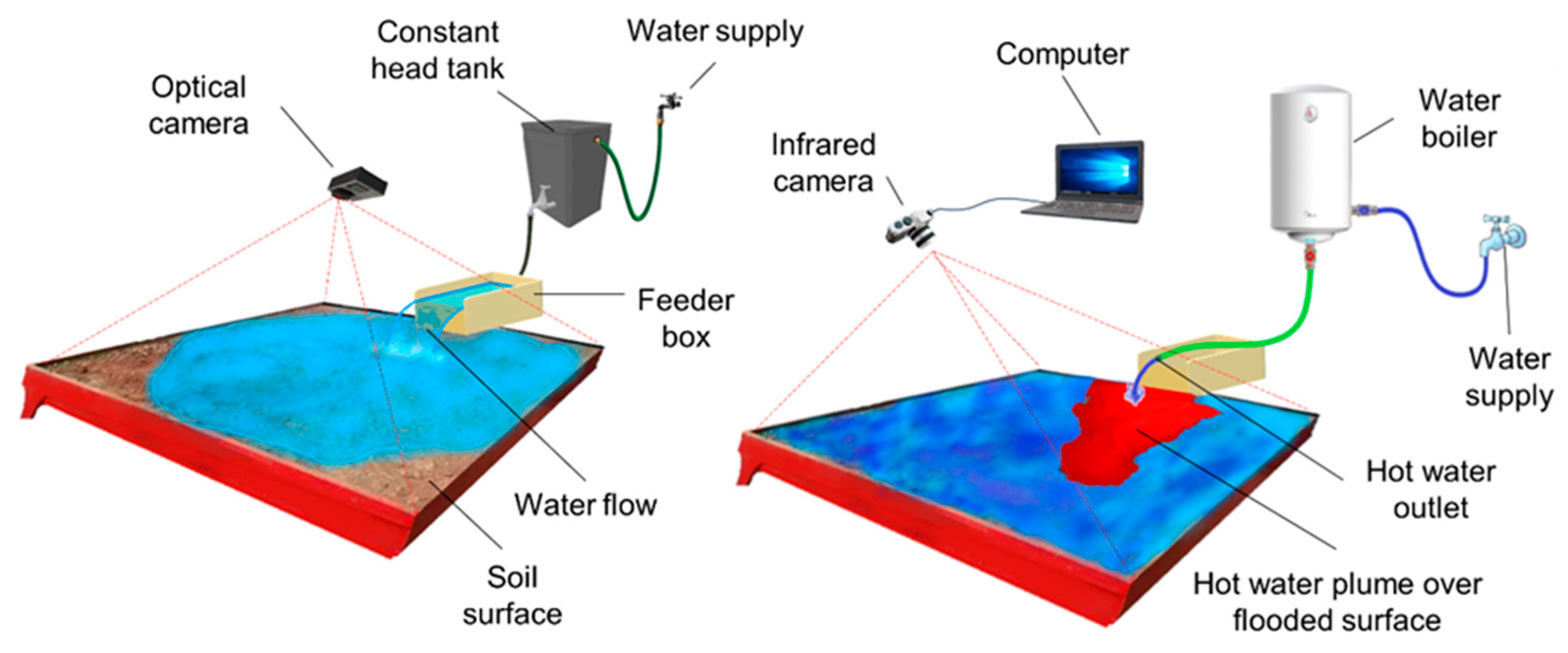
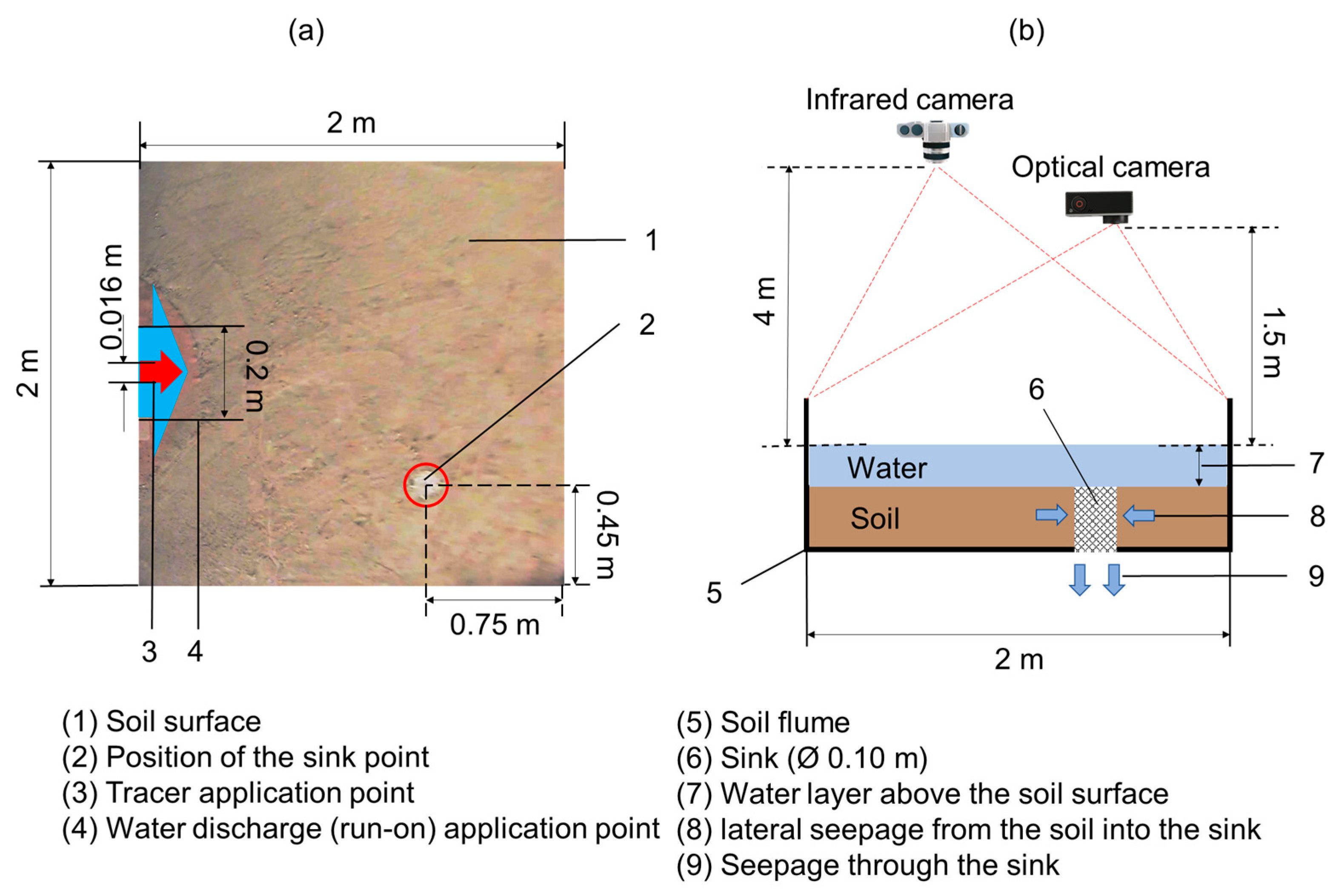
2.1. Laboratory Setup

In this study, the experiments were carried out in the laboratory using a square soil flume of 2 × 2 m². The flume had a horizontal soil surface. Upstream of the flume, a water supply system was installed, which consisted of a constant head tank and a feeder box. This system allowed for the application of a constant flow of 0.14 L/s over the soil surface in the flume. The constant head tank was filled with tap water from the laboratory supply system, with the following properties: conductivity, 75.9–150 µS/cm at 20 °C; pH, 6.5–7.3; turbidity, <1.1 NTU; O₂, 1.0–3.7 mg/L; and total hardness, 21.4–33.3 mg CaCO₃/L [35]. A PVC hose, connected to a water boiler, was used for the controlled supply of hot water (thermal tracer) during the experiments. The hose outlet was placed on top of the feeder box, enabling the application of the tracer at the same point as the water run-on. Additionally, other materials, such as cameras (optical and infrared) and a computer, were included in this experimental setup. More details on the materials and variables used are described in the following subsections. The laboratory setup for the two-phase procedure is schematically illustrated in Figure 1.

2.2. Soil and Sink Characteristics

The soil used in the flume experiments was collected (40°10′46.9″ N, 8°24′54.4″ W) from the right bank of the River Mondego, on the outskirts of the city of Coimbra, Portugal, and has been used in previous studies, e.g., [14,29]. This type of soil has a sandy-loam texture, with sand, silt, and clay contents of 79%, 10%, and 11%, respectively, and a brownish color. To prepare the flume, air-dried soil was manually placed in the flume. The soil was gently compacted using a plate and a rubber hammer to achieve homogenous compaction and a uniform thickness of 0.10 m. Subsequently, a circular sink point with a diameter of 0.10 m was created within the soil flume. To achieve this, a cylinder of soil was removed and, depending on the experimental scenario, filled with either sand or gravel to form the sink. Both sand and gravel exhibited higher permeability compared to the original soil of the flume, which had a saturated hydraulic conductivity of 0.007 mm/s (

Table 1. Experimental scenarios concerning the characteristics of the sink and tracer discharge.

Scenario	Sink Material	Permeability	Saturated Hydraulic Conductivity (mm/s)	Tracer Discharge (L/s)
a	Sand	Low	0.24	0.025
b	Sand	Low	0.24	0.035
c	Gravel	High	2.02	0.025
d	Gravel	High	2.02	0.035

). The saturated hydraulic conductivity of the soil, sand, and gravel was measured using a permeameter. Seepage from the bottom of the flume was restricted to the area of the sink. Nevertheless, lateral seepage within the soil layer into the sink also added to the overall seepage discharge from the bottom of the flume.

Figure 2 offers top and side views of the soil flume, emphasizing the sink’s location and dimensions, lateral seepage from the soil layer into the sink, vertical seepage from the bottom of the flume, and the position of the cameras.

2.3. Video Recording System

2.3.1. Flooding of the Soil Surface

During the flooding process, the movement of water flowing over the soil surface was captured using a GoProHERO3 (GoPro, Inc., San Mateo, CA, USA) optical camera with an optical resolution of 1920 × 1080 pixels. The camera was positioned 1.5 m above the maximum water level, as shown in Figure 2.

2.3.2. Tracer Application

To detect the sink, hot water was used as a thermal tracer. The water was heated using a boiler equipped with a pressure regulator in the outlet to maintain a consistent discharge. Two different discharges were chosen to achieve various experimental scenarios (as outlined in Table 1). The tracer discharge was measured using the volumetric method.

Thermograms were captured using a FLIR DUO PRO R infrared camera (FLIR Systems Inc., Wilsonville, OR, USA) with a thermal resolution of 336 × 256 pixels. The camera had an accuracy of +/−5 °C, or 5% of the readings, within the −25 °C to +135 °C range; a thermal sensitivity (NETD) of 50 mK; and a spectral range of 7.5–13.5 μm. Both the infrared camera and the optical camera were mounted on tripods positioned above the soil surface. Due to their technical specifications, the infrared camera was installed 4 m above the soil surface and connected to a computer for real-time observation of thermal images during the experiment, while the optical camera was placed 1.5 m above the soil surface. These camera heights ensured the recording of the entire flume area.

2.4. Experimental Procedure

2.4.1. Flooding of the Soil Surface

Once the soil flume was prepared, the experiment began with the application of overland flow (run-on) with a constant discharge of 0.14 L/s over the soil surface through the water supply system. The run-on continued until complete flooding occurred, which was indicated by a water depth of roughly 0.015 m above the soil surface. This process was repeated for the sand-and-gravel sink point cases. The entire flooding phase was recorded, as described in Section 2.3.1, for further video and image analysis.

2.4.2. Tracer Application

After the flooding process was completed, water heated to 70 °C was introduced into the flooded area from the boiler. A continuous supply of the thermal tracer was then applied at the identified point within the flume (Figure 2), maintaining a consistent discharge throughout each experimental scenario (Table 1). All tracer application scenarios were recorded separately during the entire experimental phase.

It is worth noting that during the tracer application period, the water level above the soil surface was not constant due to differences between the tracer discharges and sink seepage, with the application duration ranging from 240 s to 350 s.

2.5. Image Processing

The MATLAB R2020b image processing toolbox and Microsoft Video Editor version 3.1.11120.0 were used to analyze the real video frames. FLIR Thermal Studio^® version 1.9.28 thermography software was used to import, edit, and analyze thermal images.

2.5.1. Flooding Process

From the videos recorded during the flooding process, snapshots were taken at certain time intervals and cropped to encompass the soil flume section. Afterward, these cropped snapshots were converted into binary grayscale images, where only black and white colors were present. This conversion allowed for the precise calculation of the wetted area and wetted perimeter within the flume throughout the entire flooding phase. Also, snapshots were captured at specific instances during the experiment: (1) when seepage from the bottom of the flume started, (2) when the soil surface within the flume reached 100% wetness, and (3) when the flume was flooded to a predetermined depth of 0.015 m.

2.5.2. Sink Detection Method

The sink detection method was based on tracking the leading edge of the tracer’s plume over time. The sink detection method using the thermograms for each scenario consisted of the following steps (Figure 3):

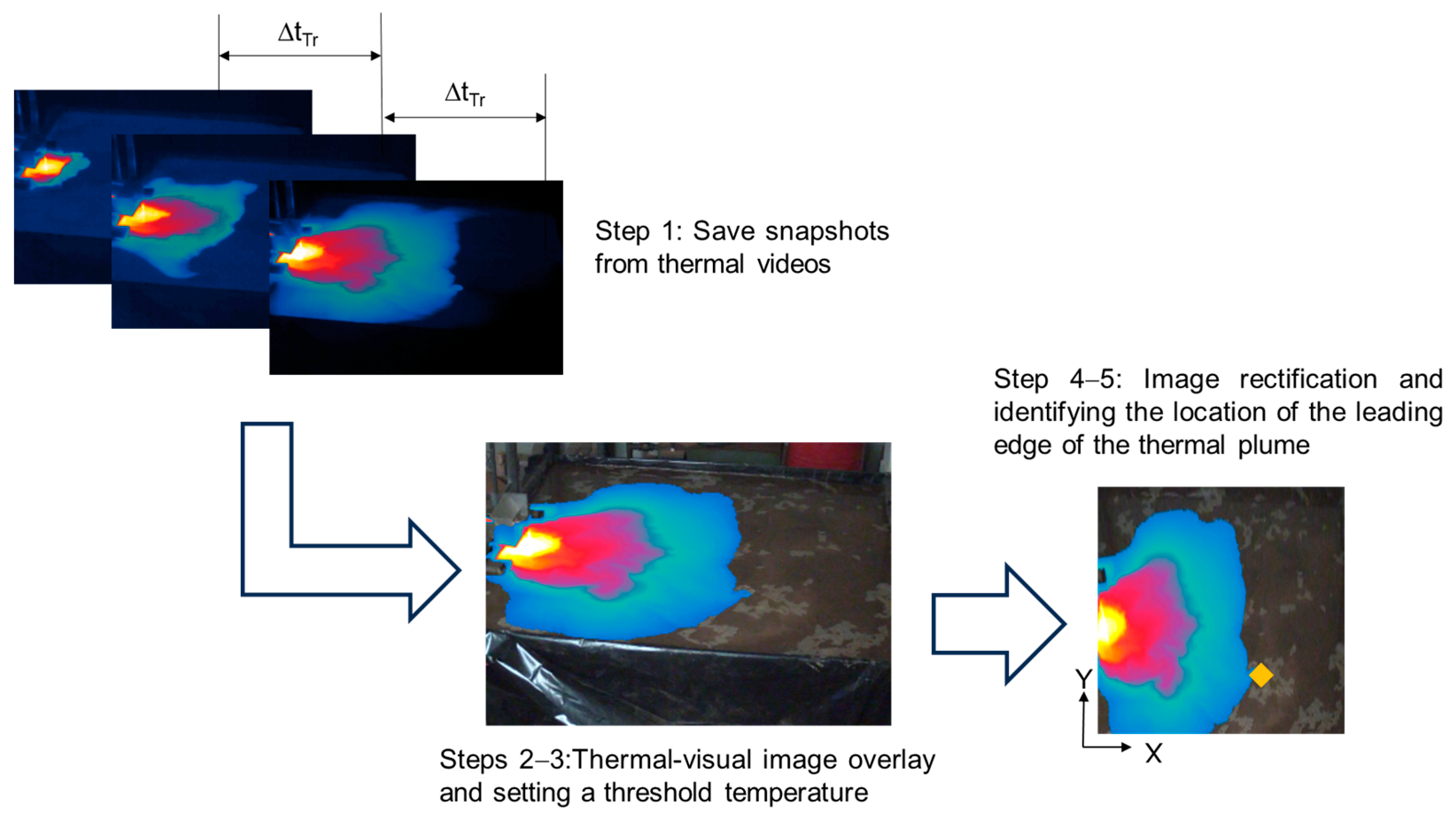
• Snapshots from the thermal videos were saved from time t₀, when the tracer was applied to the flooded area, with a time lapse of Δt_TR.
• The FLIR DUO R infrared camera’s ability to record dual images enabled overlaying the thermal and real images on each other to obtain a clear vision of the flume and the thermal diffusion in the water layer over the soil surface.
• For each series of thermographs, a threshold temperature (τ) was established at 1 °C above the maximum temperature of the water observed in the flume before applying the tracer at time t₀. This threshold temperature is used to separate the temperatures associated with the tracer plume from its surroundings. It helps identify pixels with temperature values exceeding the threshold temperature, effectively distinguishing them from the surrounding temperatures, which include pixels with temperature values below this threshold.
  The selection of an appropriate threshold temperature is crucial. A threshold equal to or lower than the water temperature within the flume where the sink is located would make it difficult to distinguish the thermal plume from its surroundings, as the entire image would appear uniformly colored. Conversely, setting the threshold too high (close to the maximum tracer temperature) would prevent observing the plume when it reaches the sink, as the temperature of its leading edge would have decreased below the tracer temperature by that point. In this study, a threshold of 1 °C above the maximum water temperature in the flume was sufficient to detect the movement of the thermal plume toward the sink.
• The thermal images were recorded at vertical and horizontal distorted angles. Therefore, to precisely determine the position of the leading edge of the tracer plume within the flume, these raw images were rectified and cropped to encompass the soil flume section. A computer-vision-based image rectification method known as Homography (matrix) was used to correct perspective distortion in the raw images, transforming non-parallel lines (due to the perspective) into a straightened version where lines are parallel [36,37]. This adjustment facilitates accurate distance measurements and ensures precise spatial analysis. The coordinates of the four corners of the soil flume were used in this approach for rectifying the raw images. This method transformed the distorted coordinates of the raw images into real metric coordinates using the dimensions of the flume as a reference.
• In each rectified image, the location of the tracer’s leading edge was determined starting from the image at time t₁ (t₀ + Δt_TR). The leading edge of the tracer’s plume was considered the furthest pixel in the X-axis direction (see Figure 3), with a temperature value above the threshold temperature. This process continued until the location of the leading edge was roughly the same (less than 0.1 m in both X-axis and Y-axis directions) in the last two images (e.g., from time t to t + Δt_TR), indicating that the tracer had reached the sink point. It was assumed that when the leading edge of the thermal tracer plume reached the sink point, the tracer started draining (seepage); therefore, the tracer’s leading-edge location remained approximately constant over time from that moment onward. Thus, this location was considered to be the location of the sink point in the flume.
  Each step was individually analyzed, and all procedures in each step were carried out using the MATLAB image processing toolbox and custom codes.

The objective of this study was to test the capability of thermal tracing in detecting sink points. A tracer temperature of 70 °C was selected to ensure distinct differentiation between the tracer plume and the water in the flume. This paper does not delve into the detailed exploration of how variations in tracer temperature may impact the results.

For assessing the accuracy of the detection method used, temperature variations along a specific line (referred to as line S) extending from the tracer application point to the detected sink location were plotted at different time intervals. This information was obtained from raw (distorted) images with dimensions of 336 × 256 pixels, as thermal data could only be extracted from these images. Figure 4 illustrates a sample of the applied method.

3. Results and Discussion

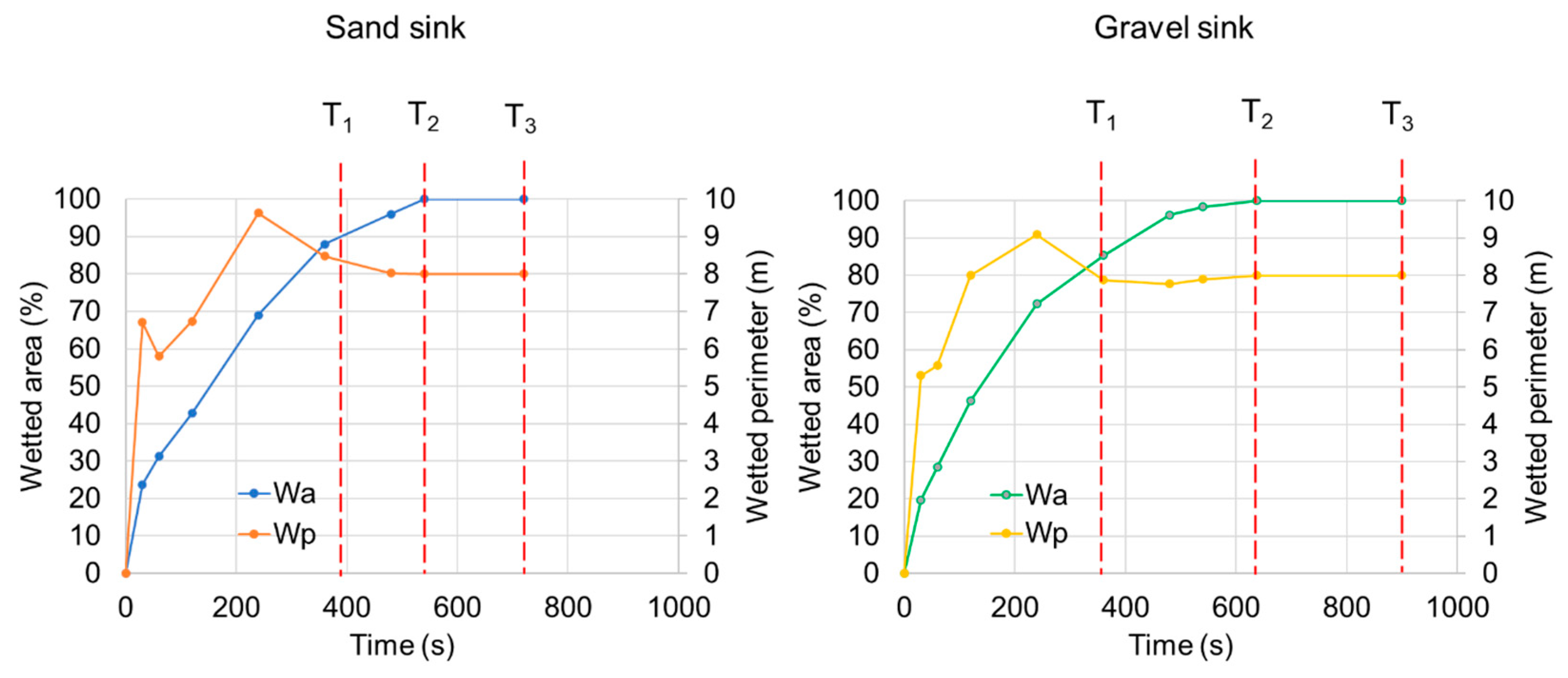
3.1. Flooding Phase

In the first part of the experiment, the soil surface wetting/flooding process, with regard to the advance of the flood wave, was induced by applying a discharge of 0.14 L/s. This process was recorded over time with an optical camera. Figure 5 illustrates the flood wave movement pattern at various time intervals within the flume, featuring the presence of sand in the sink, revealed by its lighter color.

The obtained images (Figure 5) were used to calculate the evolution of the wetted soil surface area (W_a) and the wetted perimeter (W_p) over time for both flooding cases, as depicted in Figure 6.

In both graphs, T₁ is the time when the flowing water reaches the sink and seepage starts from that point, T₂ is the time when the soil surface is 100% wet, T₃ is the time when the flume is flooded to a known depth (0.015 m), and the interval between T₂ and T₃ defines the flooding period. These parameters were calculated based on the recorded videos and the image processing method described in Section 2.5.

The arrival time of the flood wave front at the sink location (T₁) was similar for both sinks. However, there were notable differences afterward between the sand and gravel sinks. The time when the soil surface reached 100% wetness (T₂) and the time when the flooding process was completed (T₃) were both extended in the presence of gravel in the sink. This observation aligns with the fact that gravel, being more permeable compared to sand, leads to greater seepage discharge from the sink. Consequently, when the water flow reaches the gravel-filled sink, it results in an extended wetting process and a prolonged duration for the flooding to reach completion.

The information extracted from Figure 5 and Figure 6 can help us understand the flooding process and the way it was affected by the presence of sinks. When water reaches a sink point, changes in the W_a and W_p curves (Figure 6) can occur as water starts to drain, similar to what can be concluded from Figure 6. Analyzing the changes in W_a and W_p over time can help identify potential sinks in flooded areas. The variations in the curves can provide insights into the presence of sink points.

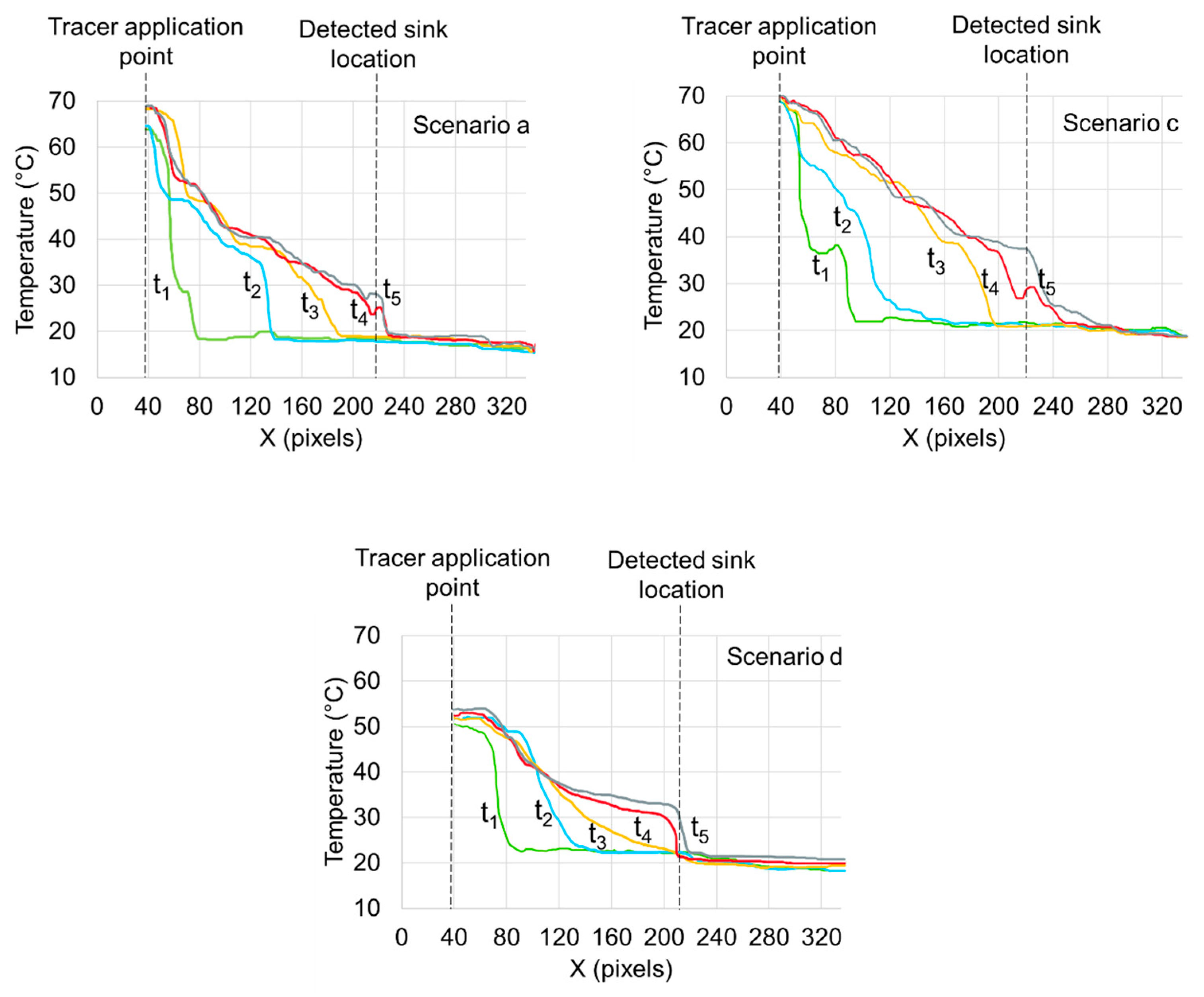
3.2. Sink Detection Phase

An illustrative example of the chronological sequence of the thermal images processed according to the method described in Section 2.5.2 is shown in Figure 7. These images were used for tracking and locating the leading-edge movement of the tracer over time. Figure 8 displays the movement of the tracer’s leading edge over time for various scenarios. Notably, it was observed that for experimental scenarios a, c, and d (Table 1), the leading edge of the tracer exhibited movement initially but eventually reached a constant position that remained unchanged over time. The consistent behavior of remaining in a fixed position helped locate the sink point. However, in scenario b, the entire flooded surface was heated by the tracer, making it challenging to detect the location of the sink. This was attributed to the presence of low-permeability soil in scenario b, coupled with high discharge of the applied tracer, resulting in rapid thermal diffusion passing over the sink making it impossible to detect the sink location using the same method. This highlights that tracer discharge can play a significant role in detecting the sink location, depending on the characteristics of the sink.

The sink was manually created in the soil flume as part of the experimental setup. In some of the optical images (e.g., Figure 5), the sink may be visible due to the materials used, which differ from the surrounding soil. However, the visibility of the sink in the images does not affect the use of the presented sink detection method. The presented thermographic tracing method relies on detecting temperature variations, with the goal of identifying the sink points regardless of whether the sink is visually detectable in the images.

The temperature variations along line S, which passes through the tracer application point and the detected sink point, were plotted over time for the studied scenarios using the method described in Section 2.5.2 (Figure 9). The purpose of presenting Figure 9 was to verify the thermal tracing sink detection method by illustrating the temperature variation from the tracer application point to the sink point before and after the tracer’s leading edge reached the sink.

As the temperature increased over time along line S due to the tracer, the heat front progressed further in the direction of the sink point. However, it is noticeable in Figure 9 that once the tracer reached the sink point at time t₄, there was an abrupt temperature drop upon crossing of the sink point. The heat front ceased to advance after time t₄, indicating that the tracer was draining at that point. The recorded location of the sink point in Figure 9 corresponds to the results obtained from the earlier sink detection method shown in Figure 7 and Figure 8. It should be mentioned that since the presented tracing method was not able to detect the sink location in scenario b, the temperature variation for scenario b is not shown in Figure 9.

4. Conclusions

The primary focus of this study, which involved laboratory experiments, was to establish and test a methodology using thermal tracers and infrared thermography to detect sink locations in shallow flooded areas. This foundational approach was tested using a homogeneous and uniform-thickness soil. Based on the experimental results, the following conclusions were drawn:

• The results highlight that tracer discharge can significantly influence the ability to detect the sink location, depending on the characteristics of the sink.
• The proposed sink detection technique successfully identified sink positions within the flooded area (laboratory flume), except in the case (scenario b) where the sink was filled with low-permeability soil and subjected to high tracer discharge.
• Sink characteristics, such as permeability, and the tracer discharge rate were crucial factors in successfully detecting the sink location.

In practical field-scale scenarios involving flooded areas, precisely estimating the location of sink leakage can enable water managers to implement effective strategies to mitigate these losses. The presented method can be a valuable tool in this process, although it may need to be adapted and refined to suit specific and more complex environmental conditions. Thus, it is recommended that future work test this technique under field conditions in shallow flooded areas of varying dimensions, with single and multiple sinks having different water losses and locations. This can include using other tracers, such as dye tracers, and using sensors like multispectral or hyperspectral cameras. While the proposed leading-edge method has shown promising results in homogeneous and uniform-soil-thickness conditions, it may face challenges in applications involving heterogeneous soils and variable soil thicknesses. Therefore, future studies should focus on improving this method to broaden its applicability. Furthermore, developing techniques to expedite the estimation of water loss due to sink leakage could be valuable. The usual process of estimating water loss from sinks can be time-consuming and resource-intensive, often relying on extensive field measurements, hydrological modeling, and complex data analysis.

References

1. Food and Agriculture Organization of the United Nations (FAO). Water for Sustainable Food and Agriculture: A Report Produced for the G20 Presidency of Germany; FAO: Rome, Italy, 2017. [Google Scholar]
2. Boyle, T.; Giurco, D.; Mukheibir, P.; Liu, A.; Moy, C.; White, S.; Stewart, R. Intelligent Metering for Urban Water: A Review. Water 2013, 5, 1052–1081. [Google Scholar] [CrossRef]
3. Luciani, C.; Casellato, F.; Alvisi, S.; Franchini, M. Green smart technology for water (GST4Water): Water loss identification at user level by using smart metering systems. Water 2019, 11, 405. [Google Scholar] [CrossRef]
4. Zaman, D.; Tiwari, M.K.; Gupta, A.K.; Sen, D. A review of leakage detection strategies for pressurised pipeline in steady-state. Eng. Fail. Anal. 2020, 109, 104264. [Google Scholar] [CrossRef]
5. Aghda, S.F.; GanjaliPour, K.; Nabiollahi, K. Assessing the accuracy of TDR-based water leak detection system. Results Phys. 2018, 8, 939–948. [Google Scholar] [CrossRef]
6. Xing, L.; Sela, L. Unsteady pressure patterns discovery from high-frequency sensing in water distribution systems. Water Res. 2019, 158, 291–300. [Google Scholar] [CrossRef] [PubMed]
7. Zhou, X.; Tang, Z.; Xu, W.; Meng, F.; Chu, X.; Xin, K.; Fu, G. Deep learning identifies accurate burst locations in water distribution networks. Water Res. 2019, 166, 115058. [Google Scholar] [CrossRef]
8. Hien, P.D.; Khoi, L.V. Application of Isotope Tracer Techniques for Assessing the Seepage of the Hydropower Dam at Tri An, South Vietnam. J. Radioanal. Nucl. Chem. 1996, 206, 295–303. [Google Scholar] [CrossRef]
9. Lee, J.Y.; Kim, H.S.; Choi, Y.K.; Kim, J.W.; Cheon, J.Y.; Yi, M.J. Sequential Tracer Tests for Determining Water Seepage Paths in a Large Rockfill Dam, Nakdong River Basin, Korea. Eng. Geol. 2007, 89, 300–315. [Google Scholar] [CrossRef]
10. Noraee-Nejad, S.; Sedghi-Asl, M.; Parvizi, M.; Shokrollahi, A. Salt Tracer Experiment through an Embankment Dam. Iranian J. Sci. Technol. Trans. Civil Eng. 2021, 45, 2787–2797. [Google Scholar] [CrossRef]
11. Thu, H.; Van, S.; Trong, H.; Viet, H.; Huu, Q.; Thi, L. Determination of the Pore Water Velocity Using a Salt Tracer Combined with Self-Potential Measurements. J. Geosci. Environ. Prot. 2023, 11, 15–27. [Google Scholar] [CrossRef]
12. Abrahams, A.D.; Parsons, A.J.; Luk, S.H. Field measurement of the velocity of overland flow using dye tracing. Earth Surf. Process. Landforms 1986, 11, 653–657. [Google Scholar] [CrossRef]
13. Abrantes, J.R.; Moruzzi, R.B.; Silveira, A.; de Lima, J.L.M.P. Comparison of thermal, salt, and dye tracing to estimate shallow flow velocities: Novel triple-tracer approach. J. Hydrol. 2018, 557, 362–377. [Google Scholar] [CrossRef]
14. de Lima, J.L.M.P.; Zehsaz, S.; de Lima, M.I.P.; Isidoro, J.M.; Jorge, R.G.; Martins, R.G. Using Quinine as a Fluorescent Tracer to Estimate Overland Flow Velocities on Bare Soil: Proof of Concept under Controlled Laboratory Conditions. Agronomy 2021, 11, 1444. [Google Scholar] [CrossRef]
15. Zehsaz, S.; de Lima, J.L.M.P.; de Lima, M.I.P.; Isidoro, J.M.; Martins, R. Estimating Sheet Flow Velocities Using Quinine as a Fluorescent Tracer: Bare, Mulched, Vegetated and Paved Surfaces. Agronomy 2022, 12, 2687. [Google Scholar] [CrossRef]
16. Zhang, G.H.; Luo, R.T.; Cao, Y.; Shen, R.C.; Zhang, X.C. Correction factor to dye-measured flow velocity under varying water and sediment discharges. J. Hydrol. 2010, 389, 205–213. [Google Scholar] [CrossRef]
17. Kantoush, S.A.; Schleiss, A.J.; Sumi, T.; Murasaki, M. LSPIV implementation for environmental flow in various laboratory and field cases. J. Hydrol. Environ. Res. 2011, 5, 263–276. [Google Scholar] [CrossRef]
18. Tauro, F.; Grimaldi, S.; Petroselli, A.; Porfiri, M. Fluorescent particle tracers for surface flow measurements: A proof of concept in a natural stream. Water Resour. Res. 2012, 48, W06528. [Google Scholar] [CrossRef]
19. Tauro, F.; Piscopia, R.; Grimaldi, S. Streamflow observations from cameras: Large-scale particle image velocimetry or particle tracking velocimetry? Water Resour. Res. 2017, 53, 10374–10394. [Google Scholar] [CrossRef]
20. Lei, T.; Chuo, R.; Zhao, J.; Shi, X.; Liu, L. An improved method for shallow water flow velocity measurement with practical electrolyte inputs. J. Hydrol. 2010, 390, 45–56. [Google Scholar] [CrossRef]
21. Schuetz, T.; Weiler, M.; Lange, J.; Stoelzle, M. Two-dimensional assessment of solute transport in shallow waters with thermal imaging and heated water. Adv. Water Resour. 2012, 43, 67–75. [Google Scholar] [CrossRef]
22. Zhou, J.; Liu, G.; Meng, Y.; Xia, C.; Chen, K.; Chen, Y. Using stable isotopes as tracer to investigate hydrological condition and estimate water residence time in a plain region. Chengdu, China. Sci. Rep. 2021, 11, 2812. [Google Scholar] [CrossRef]
23. Abrantes, J.R.; de Lima, J.L.M.P.; Prats, S.A.; Keizer, J.J. Assessing soil water repellency spatial variability using a thermographic technique: An exploratory study using a small-scale laboratory soil flume. Geoderma 2017, 287, 98–104. [Google Scholar] [CrossRef]
24. Danielescu, S.; MacQuarrie, K.T.; Faux, R.N. The integration of thermal infrared imaging, discharge measurements, and numerical simulation to quantify the relative contributions of freshwater inflows to small estuaries in Atlantic Canada. Hydrol. Process. 2009, 23, 2847–2859. [Google Scholar] [CrossRef]
25. Mejías, M.; Ballesteros, B.J.; Antón-Pacheco, C.; Domínguez, J.A.; Garcia-Orellana, J.; Garcia-Solsona, E.; Masqué, P. Methodological study of submarine groundwater discharge from a karstic aquifer in the Western Mediterranean Sea. J. Hydrol. 2012, 464, 27–40. [Google Scholar] [CrossRef]
26. Tonolla, D.; Acuna, V.; Uehlinger, U.; Frank, T.; Tockner, K. Thermal heterogeneity in river floodplains. Ecosystems 2010, 13, 727–740. [Google Scholar] [CrossRef]
27. Bonar, S.A.; Petre, S.J. Ground-based thermal imaging of stream surface temperatures: Technique and evaluation. N. Am. J. Fish. Manag. 2015, 35, 1209–1218. [Google Scholar] [CrossRef]
28. Pfister, L.; McDonnell, J.J.; Hissler, C.; Hoffmann, L. Ground-based thermal imagery as a simple, practical tool for mapping saturated area connectivity and dynamics. Hydrol. Process. 2010, 24, 3123–3132. [Google Scholar] [CrossRef]
29. de Lima, J.L.M.P.; Abrantes, J.R. Using a thermal tracer to estimate overland and rill flow velocities. Earth Surf. Process. Landf. 2014, 30, 1293–1300. [Google Scholar] [CrossRef]
30. de Lima, R.L.; Abrantes, J.R.; de Lima, J.L.M.P.; de Lima, M.I.P. Using thermal tracers to estimate flow velocities of shallow flows: Laboratory and field experiments. J. Hydrol. Hydromech. 2015, 63, 259. [Google Scholar] [CrossRef]
31. Soliman, A.S.; Rahman, M.E.A.; Heck, R.J. Comparing time-resolved infrared thermography and X-ray computed tomography in distinguishing soil surface crusts. Geoderma 2010, 158, 101–109. [Google Scholar] [CrossRef]
32. Shahraeeni, E.; Or, D. Thermo-evaporative fluxes from heterogeneous porous surfaces resolved by infrared thermography. Water Resour. Res. 2010, 46, W09511. [Google Scholar] [CrossRef]
33. de Lima, J.L.M.P.; Abrantes, J.R.; Silva, V.P.; Montenegro, A.A. Prediction of skin surface soil permeability by infrared thermography: A soil flume experiment. Quant. Infrared Thermogr. J. 2014, 11, 161–169. [Google Scholar] [CrossRef]
34. de Lima, J.L.M.P.; Abrantes, J.R.; Silva, V.P.; de Lima, M.I.P.; Montenegro, A.A. Mapping soil surface macropores using infrared thermography: An exploratory laboratory study. Sci. World J. 2014, 2014, 8845460. [Google Scholar] [CrossRef] [PubMed]
35. Águas de Coimbra. Quality Control of Water Intended for Human Consumption—Municipality of Coimbra—Boavista Supply Area—1st Semester 2020; Technical Report; Águas de Coimbra: Coimbra, Portugal, 2020. (In Portuguese) [Google Scholar]
36. Hartley, R.; Zisserman, A. Multiple View Geometry in Computer Vision, 2nd ed.; Cambridge University Press: Cambridge, UK, 2004. [Google Scholar]
37. Szeliski, R. Computer Vision: Algorithms and Applications; Springer Nature: Berlin/Heidelberg, Germany, 2022. [Google Scholar]
Figure 1. Schematic illustration of the laboratory setups (two-phase procedure). First phase (left): run-on water application on the soil surface; and second phase (right): tracer application in the flooded area.
Agriculture 14 01366 g001
Figure 2. Soil flume and camera and sink positions: (a) top view (photograph of the flume surface, with dimensions) and (b) side-view sketch (not to scale) with cameras.
Agriculture 14 01366 g002
Figure 3. Step-by-step image processing sink detection method using thermal videos.
Agriculture 14 01366 g003
Figure 4. Sample of temperature variations along line S. This line extended from the tracer application point to the sink location.
Agriculture 14 01366 g004
Figure 5. Wetting patterns over time during the flooding of the 2 × 2 m2 area. The sink can be identified in the figures by its lighter color due to its characteristics, such as sand (see Figure 1 and Figure 2). Flooding started at time t0.
Agriculture 14 01366 g005
Figure 6. Wetted area and perimeter of the soil surface over time due to flooding for a sink filled with sand (left) and a sink filled with gravel (right).
Agriculture 14 01366 g006
Figure 7. Sample of rectified thermal images with a defined threshold temperature of τ = 23 °C and a time lapse of ΔtTR = 70 s for experimental scenario a.
Agriculture 14 01366 g007
Figure 8. The tracer’s plume leading-edge location (red squares) and its movement path (blue lines) over time for different experimental scenarios. Time t0 is when the tracer was applied.
Agriculture 14 01366 g008
Figure 9. Temperature variation along line S (see Figure 4), over time, for scenarios a, c, and d.
Agriculture 14 01366 g009