Unveiling Wheat’s Future Amidst Climate Change in the Central Ethiopia Region

Abstract

Quantifying how climatic change affects wheat production, and accurately predicting its potential distributions in the face of future climate, are highly important for ensuring food security in Ethiopia. This study leverages advanced machine learning algorithms including Random Forest, Maxent, Boosted Regression Tree, and Generalised Linear Model alongside an ensemble approach to accurately predict shifts in wheat habitat suitability in the Central Ethiopia Region over the upcoming decades. An extensive dataset consisting of 19 bioclimatic variables (Bio1–Bio19), elevation, solar radiation, and topographic positioning index was refined by excluding collinear predictors to increase model accuracy. The analysis revealed that the precipitation of the wettest month, minimum temperature of the coldest month, temperature seasonality, and precipitation of the coldest quarter are the most influential factors, which collectively account for a significant proportion of habitat suitability changes. The future projections revealed that up to 100% of the regions currently classified as moderately or highly suitable for wheat could become unsuitable by 2050, 2070, and 2090, illustrating a dramatic potential decline in wheat production. Generally, the future of wheat cultivation will depend heavily on developing varieties that can thrive under altered conditions; thus, immediate and informed action is needed to safeguard the food security of the region.

1. Introduction

Climate change is one of the major threats that humankind faces with risks to future global food security [1,2]. With the accelerated increase in atmospheric CO₂ to the expected 700 μL L⁻¹ by the end of the 21st century [3], the threat to the agricultural sector is expected to be much more severe [2,4,5,6,7,8]. Climate change affects agricultural activities through changes in phenological events, the suitability of land for crops, the increasing invasion risk of weed species, and fluctuations in grain yield [9,10]. Notably, higher temperatures and higher concentrations of CO₂ caused by climate change affect the existing crop suitability of regions and agricultural landscapes [11,12] and consequently affect food systems in various ways [13]. To understand the consequences of these changes for food security, quantitative analysis of the potential distributions of crop species and the environmental factors affecting their production under current and future climate scenarios plays a central role.

Species distribution models (SDMs) are powerful tools for identifying the potential areas of suitable species habitats by exploring the relationships between geographical species records (e.g., species occurrences) and corresponding environmental variables [14]. SDMs are widely used for an array of applications in ecology, natural resource conservation, and climate change impact studies. However, the increasing availability of SDMs and their varying capacity to establish relationships between species and environmental variables makes it difficult to choose the best method for conducting the models [12,15]. To account for uncertainties and increase the predictive power of individual models, the ensemble modelling technique was suggested to be the best alternative for determining the current and future distributions of species [16,17]. By combining all the individual models, the ensemble model produces a single output with a more accurate and robust prediction.

As the most widely grown and third largest crop in the world, wheat plays a significant role in global food security. Within Africa, Ethiopia stands out as the second-largest wheat producer [18]. In 2022, the country cultivated wheat across a total cropland area of 2.1 Mha, yielding approximately 6.23 million tons. Given that almost all food imports in Ethiopia consist of wheat, the government has prioritised wheat production through initiatives such as crop area expansion, implementation of irrigation systems, and yield gap closure through agroclustering of farmers [19]. Despite the significant challenge posed by climate change to crop productivity and land suitability, documented successes in the wheat sector underscore the importance of these strategies [20]. Recent reports suggest that the dry-season wheat irrigation project is showing commending results [20], and Prime Minister Abiy Ahmed has received the prestigious FAO-Agricola medal in recognition of his dedication to wheat self-sufficiency and food security. The irrigation initiative has continued to expand in 2023 and 2024. Nevertheless, the looming threat of climate change to land suitability for wheat cultivation is becoming increasingly apparent, necessitating finer-scale studies beyond the national level [21,22]. In light of this concern, our study employs the best available methods to conduct land suitability assessments and identify suitable habitats for wheat under current and future climate scenarios in the Central Ethiopia Region (CER).

The CER emerged as a significant surplus wheat producer and one of the hotspots for climate change impacts [23]. Given the region’s pivotal role in wheat initiatives, understanding wheat land suitability in the region becomes imperative [19]. Despite its importance, the potential distribution range of wheat and geographic areas vulnerable to climate change remain unidentified within the region. More importantly, in Ethiopia, the wheat occurrence points are collected from relatively accessible locations and only limited geolocations exist. In particular, in the study area very few non-randomly collected sample points exist. Thus, there is a strong tendency toward sample bias, which considerably influences the accuracy of wheat distribution prediction in the study area. Consequently, this study aimed to address this gap by pursuing the following objectives: (1) to survey wheat occurrence points and examine the current distribution of wheat under current climate conditions in the CER; (2) to understand the role of environmental variables affecting the geographical distribution of wheat; and (3) to predict the potential geographical distribution and spatial alterations of wheat under two climate change scenarios. To meet these objectives, we employed four machine-learning algorithms alongside their ensemble model. We utilised different sets of emission scenarios driven by different socioeconomic assumptions (SSP2–4.5 and SSP5–8.5) for the years centered on 2030, 2050, 2070, and 2090, leveraging the ensemble of five global circulation models (ACCESS-CM2, HadGEM3-GC31-LL, MIROC6, MPI-ESM1-2-HR, and CMCCESM2). In connection with this, we hypothesised that the suitable land area for wheat in the CER would decline under the influence of global climate change, underscoring the necessity for adaptation strategies. The insights derived from this study offer crucial guidance for policymakers, facilitating their efforts to expand wheat production both temporally and spatially within the country.

2. Materials and Methods

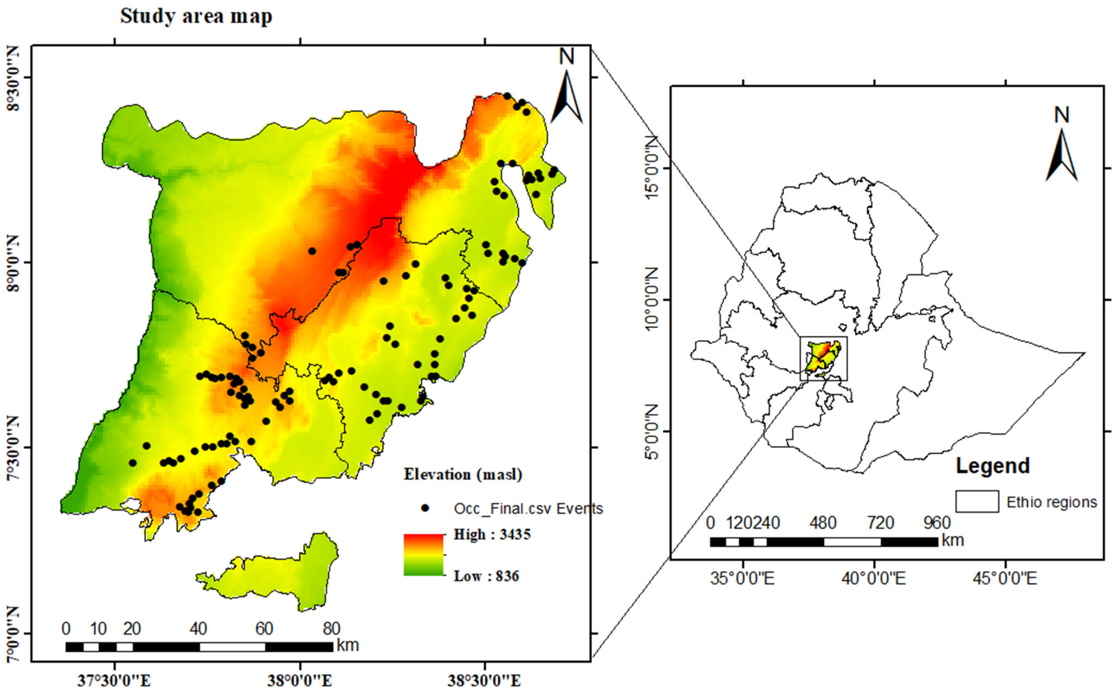
2.1. Study Area Description

This study was conducted in three major wheat-producing zones (Hadya, Silte, and Gurage) in CER (Figure 1). The study area has an altitude ranging from 836 to 3435 m.a.s.l. and is located between 7°05′78″ and 8°45′76″ N and 37°34′95″ and 38°71′60″ E. The total land area is 12,203 square kilometers. From an agroecological point of view, the study area comprises lowlands, dry midlands, wet midlands, and highlands. This diverse agroecology enables the area to diversify its livelihood systems. The major livelihood types include Meher livelihood type, Belg livelihood type, and agropastoralism. The major crops grown in the area include wheat, maize, teff, sorghum, barley, enset, and vegetables. In terms of rainfall occurrence, there are three distinct seasons, locally known as Belg, Kiremt, and Bega. The Belg (small rain) extends from February to May; the Kiremt season (the main rain) mostly occurs from June to September and is crucial for Meher livelihood type, and the Bega (dry) season extends from October to January. The amount of rainfall received during the three seasons varies significantly. The Belg and Kiremt seasons contribute approximately 90% of the annual climatological mean rainfall and thus control agricultural production in the study area. While Kiremt is the main rainy season for the cultivation of most crops in most parts of the region, Belg season rainfall is equally significant for growing early-maturing and long-season crops, and it is a source of water for growing animal pastures and is the source of the dominant livelihood type in the southern part of the study area.

2.2. Species Occurrence Points or Sample Location Data

The wheat occurrence points at Addis Ababa University’s National Herbarium and the Ethiopian Biodiversity Institute are very limited, and databases such as https://www.cabi.org/cpc/ (accessed on 7 October 2023), www.gbif.org (accessed on 8 October 2023), and www.idigBio.org (accessed on 7 October 2023) completely lack wheat occurrence points for the Central Ethiopia Region. Thus, the species records for the study were generated through a survey of potential wheat-producing areas. A handheld global positioning system (GPS, Garmin 72 H) was utilised to record the geographic positions within the sampling area, where 156 presence-only points were collected. The survey records covered Sankura, Mito, Dalocha, Hulbareg, Silti, and Lanfuro woreda of the Silte Zone. We also surveyed Sodo, Mareko, Gumer, and Indegay of the Gurage Zone and Duna, Misha, Soro, Lemo, Alemo, and Gibe woreda of the Hadiya Zone. To avoid the possibility of potential bias in obtaining clustered spatial records, the repeatability of geocoordinates was removed by rarefying the occurrence points to one observation per 1 km² cell using the SDM toolbox implemented in Arcmap 10.7. Finally, 117 occurrence points remained for analysis. The coordinate system was WGS84.

2.3. Environmental Variables

Bioclimatic variables represent important explanatory variables for understanding the relationships between the geographical distribution of various species and environmental variables. The historical climate dataset (1970–2000) was obtained from Worldclim version 2.1 and used as a baseline [24]. The environmental variables include 19 gridded Bioclimatic variables, with a spatial resolution of 30 arc-seconds (~1 km²) (http://www.worldclim.org/version2.1, accessed on 22 November 2023). The first 11 of the 19 bioclimatic variables (Bio1 to Bio11) were classed into the temperature group, and the other variables (Bio12 to Bio19) were grouped into the precipitation group (see

Table 1. List and description of environmental variables used in the modelling of wheat in the CER.

Code	Name	Units
Bio1	Annual Mean Temperature	°C
Bio2	Mean Diurnal Range (Mean of monthly (max temp–min temp))	°C
Bio3	Isothermality (Bio2/Bio7) (×100)	-
Bio4	Temperature Seasonality (standard deviation ×100)	°C
Bio5	Max Temperature of Warmest Month	°C
Bio6	Min Temperature of Coldest Month	°C
Bio7	Temperature Annual Range (Bio5-Bio6)	°C
Bio8	Mean Temperature of Wettest Quarter	°C
Bio9	Mean Temperature of Driest Quarter	°C
Bio10	Mean Temperature of Warmest Quarter	°C
Bio11	Mean Temperature of Coldest Quarter	°C
Bio12	Annual Precipitation	Mm
Bio13	Precipitation of Wettest Month	Mm
Bio14	Precipitation of Driest Month	Mm
Bio15	Precipitation Seasonality (Coefficient of Variation)	Fraction
Bio16	Precipitation of Wettest Quarter	Mm
Bio17	Precipitation of Driest Quarter	Mm
Bio18	Precipitation of Warmest Quarter	Mm
Bio19	Precipitation of Coldest Quarter	Mm
Elevation	Elevation	m.a.s.l
TPI	Topographic positioning index	-
Solar	Solar radiation	kJ m−2 day−1

Note: Bioclimatic variables in bold are variables selected for modelling of wheat land suitability after checking for collinearity.

for details). The other environmental groups included in the modelling were 12 monthly solar radiation and topographic variables (topographic positioning index and elevation). We generated individual and ensemble species distribution models (SDMs) and forecasted for the periods of 2021–2040, 2041–2060, 2061–2080, and 2081–2100. For each period, we employed an ensemble of five widely used Global Circulation Models (ACCESS-CM2, HadGEM3-GC31-LL, MIROC6, MPI-ESM1-2-HR, and CMCCESM2) from the two regularly applied SSPs in climate-change assessments, i.e., the moderate scenario (SSP2–4.5) and the worst-case scenario (SSP5–8.5) [25].

2.4. Variable Importance and Collinearity Test for Variable Selection

The bioclimatic variables were derived from interpolated datasets and they often show redundancy/multicollinearity, ultimately leading to poor or misleading model performance [16]. The correlations and dependencies of the variables affect the variable importance and make their interpretation difficult. To avoid overfitting and remove redundant environmental variables that do not provide additional information to the modelling exercise, we used the stepwise variance inflation factor (VIF) from the “usdm” R package 4.3.1. [26]. Stepwise variable selection based on VIF is the most commonly used method to address collinearity [14,27]. The VIF value of 10 (as a rule of thumb) was used as a cut-off point. The stepwise procedure selected 10 variables with a VIF of less than the threshold (Table 1).

2.5. Modelling Algorithms

The geographical distribution of wheat was predicted using four species distribution models (algorithms) implemented in the sdm, R package, which include Maximum Entropy (Maxent) [28], Random Forest (RF) [29], Boosted regression trees (BRT) [30], and the Generalised Linear Model (GLM) [31]. These SDMs are the most effective and well-approved techniques for modelling species distributions [32,33].

2.5.1. Maxent Model

The Maxent model uses existing information about a species’ geographic location range and related environmental factors to create a suitability map [28]. Maxent estimates species distribution as a probability distribution by maximising a relative-entropy objective function that compares environmental conditions at species occurrence points to a sample of background points representing the environmental condition of the study area [34]. It is one of the best-performing and most widely used SDM algorithms in practical applications because of its user-friendly interface, reliable prediction, and low computing capacity [9,35].

2.5.2. Random Forest

Random Forest (RF) is a classification or regression ensemble machine learning algorithm that builds multiple trees by using random subsets of the dataset, and subsequently aggregates the predictions generated by these individual trees [29]. It is a classification or regression tree-based model that is not sensitive to data distribution. RF stands as one of the most extensively utilised and most accurate machine learning algorithms for predicting species distributions [36].

2.5.3. Boosted Regression Trees

Boosted regression trees (BRTs), also known as stochastic gradient boosting or boosted additive trees, result from the merging of regression trees with the boosting technique [37]. BRT represents a machine-learning approach that commences with a single decision tree that undergoes multiple simple binary decisions [15,38]. BRT integrates the strengths of regression trees, which link a response to predictors through recursive binary splits, and boosting, a strategy that amalgamates numerous simple models to improve modelling accuracy. The final BRT model is an additive regression model consisting of simple trees. It performs well with a low to moderate number of presence-only data through the generation of pseudoabsences.

2.5.4. Generalised Linear Model

A generalised linear model (GLM) is an extension of the classic linear regression modelling technique that has long been a prominent algorithm in SDM studies [39]. It is a parametric approach that addresses different families of the statistical distribution of data and allows nonlinear and nonconstant variance of data. The effects of the independent variables, which are nonlinear and characterised by exponential and systematic observations, as well as rarely following normal distributions, can be rendered linear through the utilisation of an appropriate transformation method for analysis [15,31].

2.5.5. Ensemble Model

An ensemble modelling approach entails combining predictions from multiple models to reduce the inaccuracy and biases of individual model predictions. To improve modelling accuracy, a weighted averaging approach based on Area Under the Curve (AUC) statistics was employed to determine the contribution of each of the four individual models to the ensemble model. A weighted averaging approach was determined as follows:

$$\mathrm{E}={\displaystyle \frac{\sum _{\mathrm{i}=1}^{\mathrm{n}}{\mathrm{A}\mathrm{U}\mathrm{C}}_{\mathrm{i}} \mathrm{\ast } {\mathrm{M}}_{\mathrm{i}}}{\sum _{\mathrm{i}=1}^{\mathrm{n}}{\mathrm{A}\mathrm{U}\mathrm{C}}_{\mathrm{i}}}}$$

Following this, the evaluates function of R was used to determine the AUC and TSS of the ensemble, and then the predict function of the sdm was used to project the models onto current and future environmental conditions. The resulting suitability maps were converted into unsuitable, low suitability, moderately suitable, and highly suitable categories.

2.6. Evaluation of Model Performance

We used the sdm R package [14] to model and predict species distributions. The occurrence points were randomly divided into two partitions via a resampling method, called subsampling and bootstrapping method, through which 70% of the occurrence points were used for training the models and the remaining 30% of the occurrence points were used to evaluate the models. To reduce potential bias introduced by resampling, the procedure was repeated 30 times. The performance of the SDMs was assessed through the utilisation of the area under the receiver operating characteristic curve (AUC) and true skill statistics (TSS). The AUC represents the area enclosed by the receiver operating characteristic (ROC) curves within the model [40]. The ROC curve’s AUC is a commonly employed metric to evaluate the discriminatory performance of SDMs. The ROC curve plots sensitivity versus (1—specificity) across all possible thresholds between 0 and 1. The sensitivity (i.e., true positive rate) is the ratio of the number of predicted observed presences (omission errors) or true positives divided by the total number of presences (true positive plus false negatives). The specificity is the ratio of the number of predicted observed absences (commission errors) or the ratio between true negatives divided by all absences. A model is deemed to perform better than random chance if the curve is positioned above the diagonal line of no discrimination (AUC = 0.5), indicating an AUC greater than 0.5. The ROC curve of a model exhibiting flawless discriminatory ability extends from coordinate (0,0) to coordinate (0,1) and then to another corner (1,1). Generally, on the basis of the range of AUC values, a model’s performance can be interpreted as excellent (0.9–1.0), very good (0.8–0.9), good (0.7–0.8), fair (0.6–0.7), or poor (0.5–0.6) [41]. The TSS is computed by subtracting 1 from the summation of sensitivity and specificity [42]. The value of the TSS ranges from −1 to 1, where a value of zero represents a model performing the same as prediction by chance (total random error), while −1 indicates a model with a total error, and a TSS equal to 1 is a perfect model. The ensemble model was constructed using the four individual models to address the uncertainties associated with the performance and prediction of each model. The raster values were classified into suitability classes [43]. The suitability values range from 0 to 1, indicating the lowest to highest habitat suitability, respectively. The climate suitability of wheat cultivation was classified into unsuitable areas (small probability) (p < 0.05), low suitability areas (0.05 ≤ p < 0.33), moderate suitability areas (0.2 ≤ p < 0.66), and high suitability areas (p ≥ 0.66) [9,44].

3. Results and Discussions

3.1. Model Fitting and Performance

The models selected for assessing the potential distribution of wheat were highly effective across all modelling tasks. The predictive performance of the models was assessed on the basis of the AUC and TSS. The average AUC values for RF, Maxent, BRT, GLM, and Ensemble were 0.9, 0.86, 0.85, 0.85, and 0.94, respectively, which proved that the performance of all the SDMs was very good or excellent (

Table 2. Model test.

Methods	AUC	TSS
Random Forest (RF)	0.9	0.68
Maxent	0.86	0.62
Boosted regression tree (BRT)	0.85	0.6
Generalised Linear Model (GLM)	0.85	0.61
Ensemble model	0.94	0.76

). The True Skill Statistics (TSS) values were > 0.5 for all the SDMs. In the assessment metrics employed in this research, the ensemble model demonstrated the highest values, with Random Forest (RF) and Maxent following closely behind. Shabani et al. [45] proposed that a model with an AUC value exceeding 0.75 is considered robust and precise. The AUC values for all models used in this study were greater than 0.8, indicating that the models are reliable for assessing the ecological suitability and predicting the geographical distributions of wheat. Moreover, the ensemble technique resulted in a significant gain in prediction accuracy. The high AUC and TSS values also imply that the models can discriminate suitable and unsuitable wheat sites accurately [46] in the CER. A study by West et al. [47] that used species distribution models reported that RF and Maxent were the best SDM models for the prediction of invasive species. This makes the models most suitable for species distribution modelling.

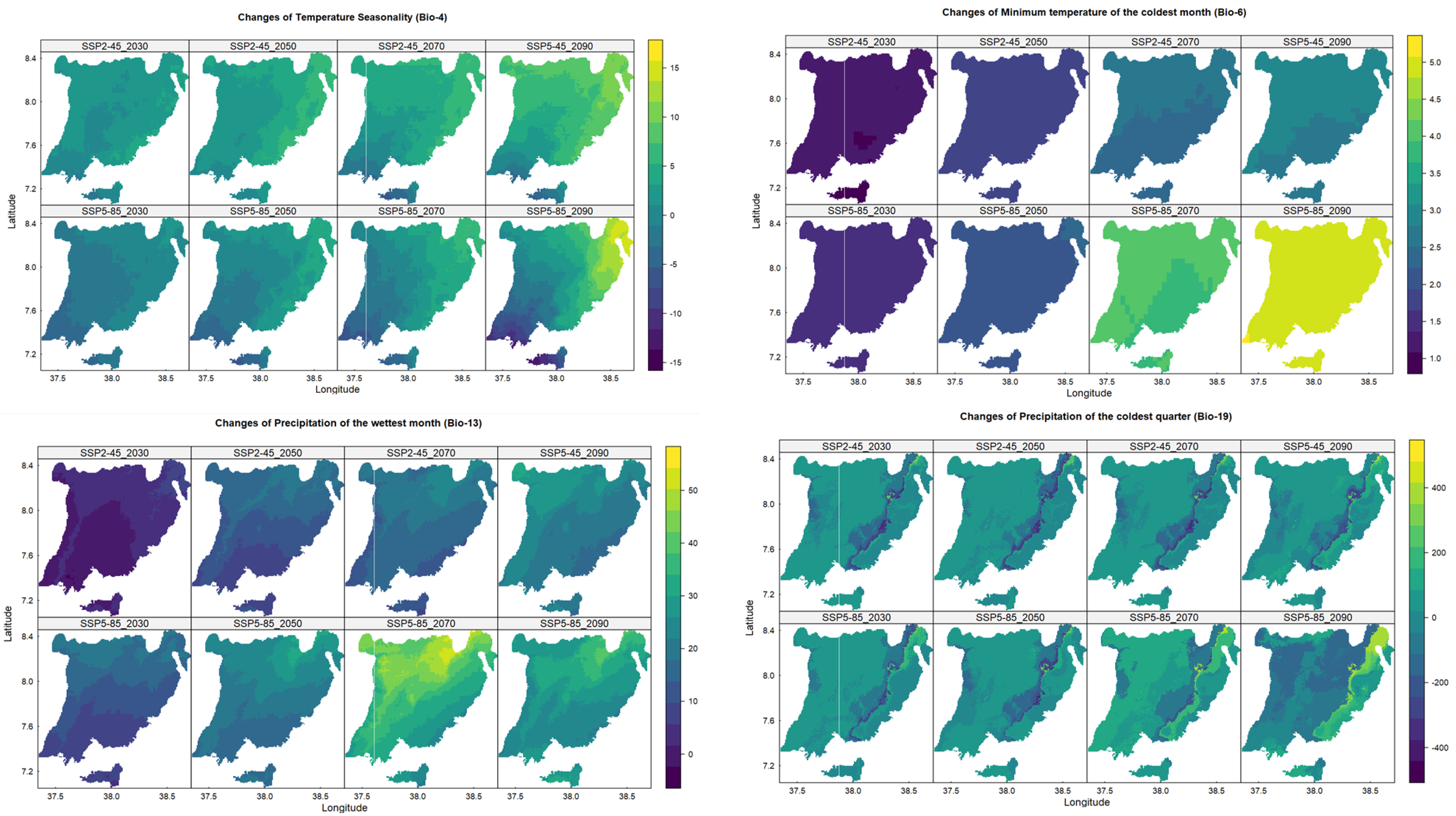
3.2. Contribution of Environmental Variables Affecting Wheat Cultivation in CER

The performances of the bioclimatic variables were similar among the modelling algorithms. The relative variable importance of ten variables was normalised to sum to 100% (

Table 3. Relative variable importance of ten variables normalised to the sum of 100% * in the Random Forest (RF), maximum entropy (Maxent), Boosted Regression Tree (BRT), and Generalised Linear Model (GLM) models.

Environmental Variables	RF	Maxent	BRT	GLM	Mean
Mean diurnal range (Bio2)	9.1	13.1	2.8	13.8	9.7
Iso-thermality (Bio2/Bio7) (×100) (Bio3)	5.9	6.7	3.0	9.0	6.2
Temperature Seasonality (standard deviation ×100) (Bio4)	11.8	15.4	15.0	15.0	14.3
Min Temperature of Coldest Month (Bio6)	12.4	23.2	9.7	22.2	16.9
Precipitation of wettest month (Bio13)	23.1	25.7	34.3	31.7	28.7
Precipitation of driest quarter (Bio17)	3.2	2.6	0.8	2.5	2.3
Precipitation of warmest quarter (Bio18)	3.9	4.0	1.5	1.3	2.7
Precipitation of coldest quarter (Bio19)	18.1	6.1	25.6	1.7	12.9
Solar Radiation	8.3	2.4	3.6	2.5	4.2
Topographic positioning index (tpi)	4.3	0.8	3.6	0.4	2.3
Total sum	100	100	100	100	100

* Normalisation was used to make the metrics’ relative assessments comparable.

and Figure 2). The precipitation of the wettest month (Bio13) had the most important explanatory power in predicting wheat cultivation areas. The respective significance values of Bio13 were 23.1% for RF, 25.7% for Maxent, 34.3% for BRT, and 31.7% for GLM. The next most significant factor is Precipitation of the Coldest Quarter (Bio19) for RF (18.1%) and Boosted Regression Tree (25.6%), and Minimum Temperature of the Coldest Month for Maxent (23.2%) and GLM (22.2%). Considering the mean values of all modelling exercises, the Precipitation of the Wettest Month (Bio13) is the most significant variable governing the distribution of wheat with importance scores (mean score = 28.7%), followed by the Minimum Temperature of the Coldest Month (Bio6) (mean score = 16.9%), Temperature Seasonality (Bio4) (mean score = 14.3%), and Precipitation of the Wettest Quarter (Bio19) (mean score = 12.9%). Whereas, the Topographic Positioning Index (tpi), Precipitation of the Driest Quarter (Bio17), and Precipitation of the Warmest Quarter (Bio18) are the three variables with the least importance for the modelling exercises, respectively.

In a previous study, Evangelista et al. [22] reported that climatic variables related to rainfall are the most significant factors affecting cereal yield prediction in Ethiopia. Nevertheless, in this study, variables related to both temperature (Minimum Temperature of the Coldest Month-Bio6, precipitation seasonality-Bio4), Precipitation of the Wettest month-Bio13, and Precipitation of the Coldest Quarter-Bio19 significantly influenced wheat production.

Wheat production in Ethiopia primarily occurs during the main rainy season, which typically spans from June to September. The precipitation of the wettest month (Bio13) and precipitation of the coldest month (Bio19) occur during the main rainy season indicating that the environmental conditions during this period strongly influence the distribution of wheat. Precipitation profoundly influences various stages of the crop growth cycle, including germination, tillering, anthesis, and grain filling. Similarly, temperature impacts the flowering time and thermal requirements of wheat. A warmer climate hastens crop development and alters the anthesis period, thereby affecting the yield produced. Furthermore, elevation significantly influences wheat cultivation by affecting temperature and rainfall patterns. Although elevation was initially considered to be a very important variable that influences wheat distribution in our modelling exercise, it was eventually excluded because of its strong correlation with precipitation and temperature parameters. Conversely, the role of the topographic positioning index and solar radiation in determining habitat suitability for wheat cultivation was found to be negligible. This is contrary to the finding of Yang et al. (2020) [48] in the Northern part of the country, which suggested a significant role of solar radiation in cereal production.

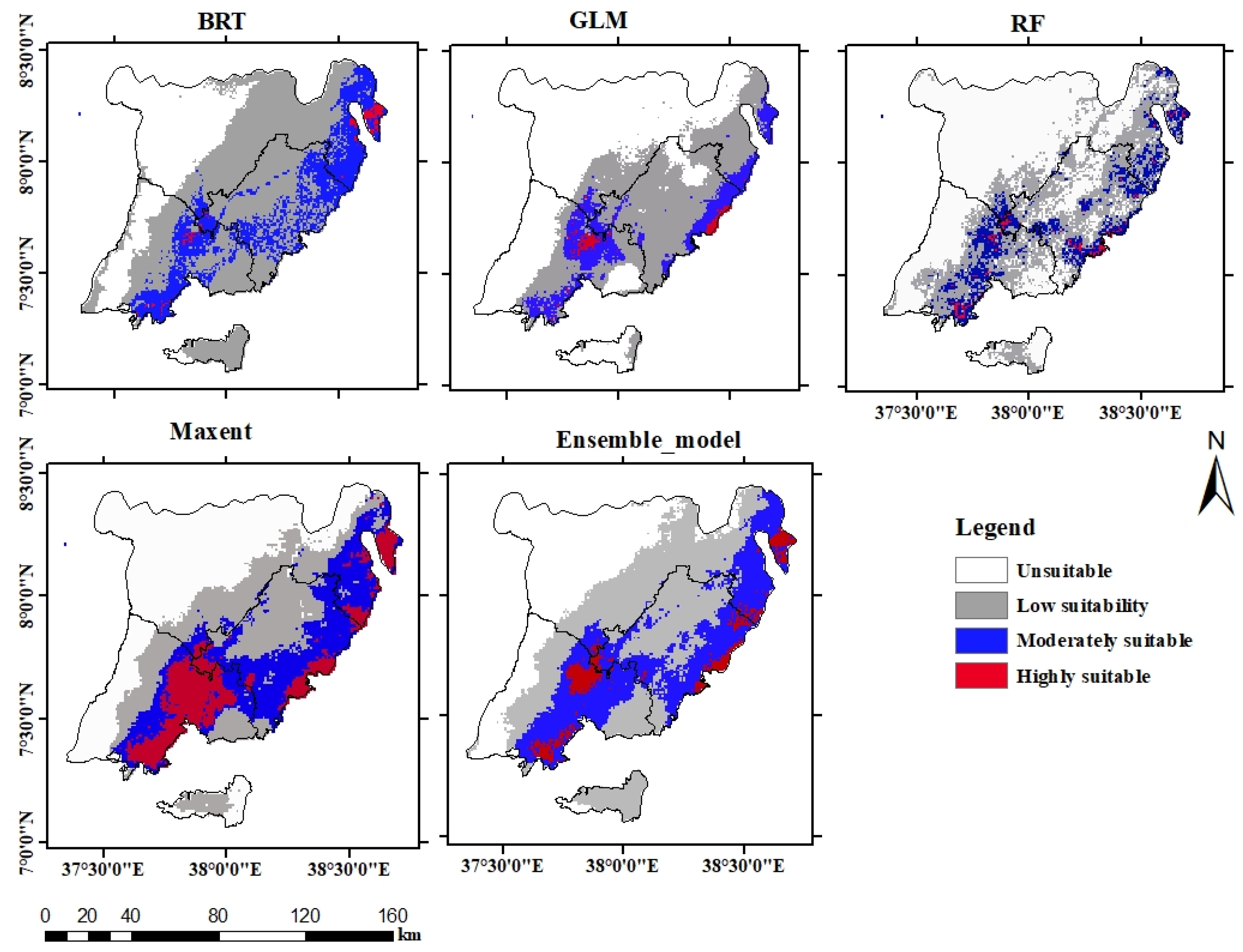
3.3. Current Climate Suitability of Wheat in the CER

The current suitability of wheat as estimated by the four modelling algorithms and their ensemble is shown in Figure 3 and

Table 4. Current wheat habitat suitability simulations (areas calculated in km² and %) by using Random Forest (RF), Maxent, Boosted Regression tree (BRT), Generalised Linear Model (GLM), and ensemble modelling approaches.

	RF		Maxent		BRT		GLM		Ensemble
	Area	%	Area	%	Area	%	Area	%	Area	%
Not suitable	6640	54	4491	37	3077	25	6058	50	3594	29
Low suitability	4000	33	3467	28	6411	33	4535	37	4947	41
Moderately suitable	1420	12	2664	22	2578	21	1451	12	3067	25
Highly suitable	143	1	1580	13	137	1	158	1	595	5

. From a total land area of 12,203 km², the ensemble model shows that 30% (3662 km²) of the current land area is highly or moderately suitable and the remaining 70% (8541 km²) is unsuitable or has low suitability for wheat production. Among the four single SDMs used in this study, the Maxent model indicated the highest share of moderately and highly suitable areas (35%, 4244 km²), and the GLM and Random Forest showed the least range of moderately and highly suitable areas, with 13% each.

The highly suitable and moderately suitable areas are located in Sodo, Meskan, Mareko, and Indegay woreda of the Gurage Zone; Mito, Wulbareg, Sankura, Lanfuro, and Silte woreda of the Silte Zone, and Duna, Soro, Mish, and Lemo woredas of the Hadiya Zone. The areas with unsuitable or low suitability are mainly found in the northwestern parts of the study area, mainly in the Gurage Zone, which was evidenced in all the models. The Maxent prediction coincides with the current potential wheat-producing areas or the sites of occurrence points, which may suggest that the Maxent is more reliable and superior in species distribution modelling than other modelling algorithms. The argument that Maxent is a more reliable tool for identifying a geographical range of species and should be considered a first modelling option becomes valid in this study [35]. Grimmett et al. [39] also suggested that Maxent is the most consistent SDM tool in terms of performance metrics and spatial prediction stability under varying sampling strategies, and should be used for scenario analysis alone or as part of an ensemble model. In fact Kaky et al. [35] suggested that Maxent will remain the dominant software to be used for the application and interpretation of results at least in developing countries, owing to its user-friendly interface and requirement of less advanced statistical modelling techniques. On the other hand, though Random Forest has the highest prediction accuracy based on AUC and TSS, its suitability maps show signs of under-prediction when compared with the actual occurrence points. The visual inspection shows that Maxent has greater similarity with the ensemble than does the random forest (Figure 3).

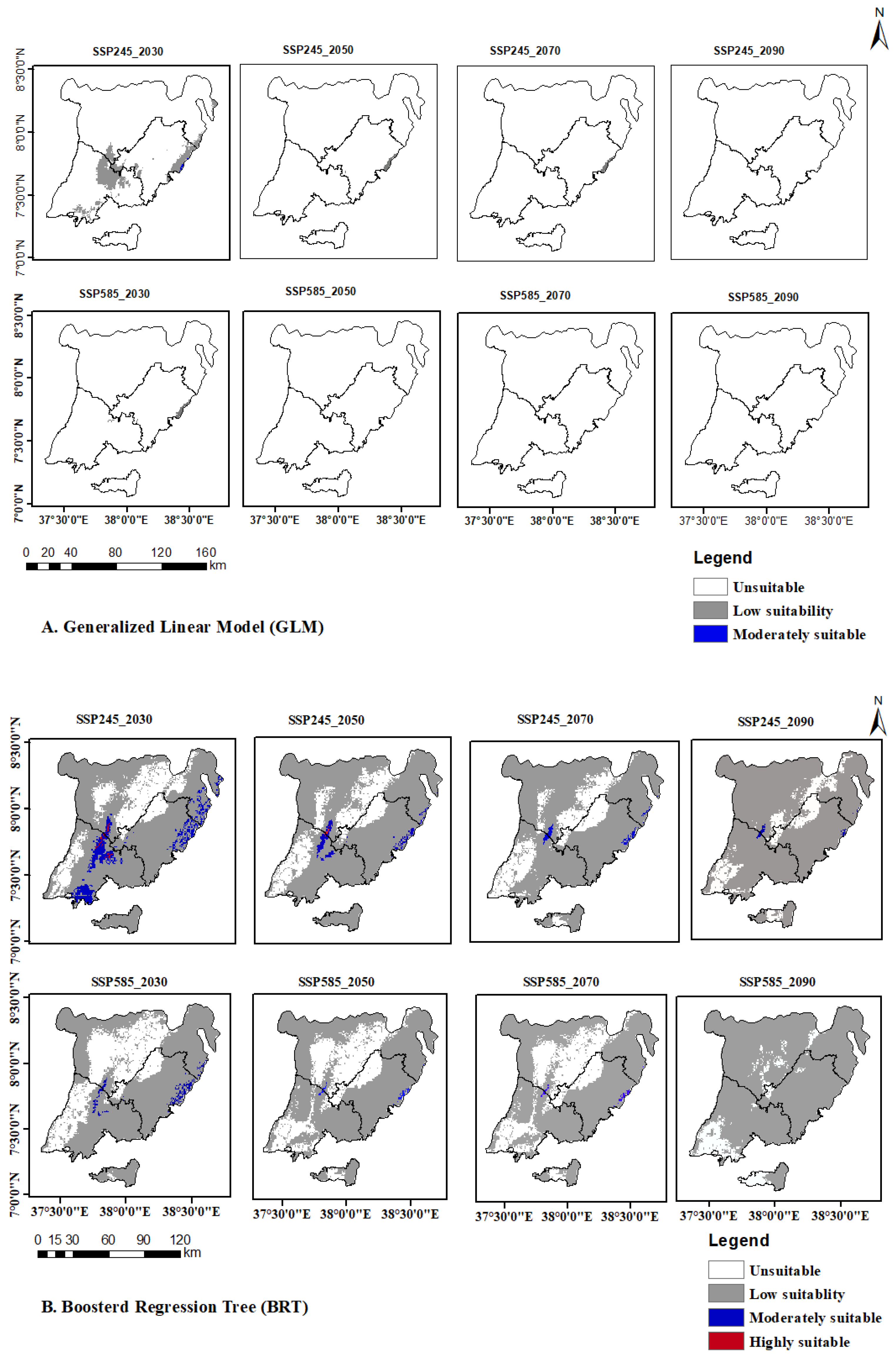
3.4. Wheat Habitat Suitability under Future Climate Scenarios

The impacts of climate change on wheat land suitability under future climate scenarios (SSP2–4.5 and SPP5–8.5) for the years 2030, 2050, 2070, and 2090 are illustrated in Figure 4A–E. The habitat suitability of wheat is expected to decline under future climate change scenarios. The extent of suitable land decline depends on the SDM model used, the shared socioeconomic pathways followed and the modelling period taken into consideration, as indicated by individual and ensemble models. All the models indicated a considerable decline in wheat habitat suitability with GLM showing a rapid and significant loss of moderately and highly suitable habitats under both scenarios in 2030 and afterwards (Figure 4). Compared with other models, the Maxent and the ensemble models resulted in relatively less highly or moderately suitable wheat habitat loss. When Maxent is used, the moderately and highly suitable area will decrease to 16.6% (SSP2–4.5) in 2030, which will further derease to 0.1% in 2070. When Maxent is used under SSP5–8.5, the moderately suitable habitat will be 0.2% in 2030 and it will further reduce to 0.1% in 2070. However, the ensemble model shows a decrease in moderately and highly suitable habitat to 7% in 2030 under SSP2–45 and to 0.3% in 2050 under SSP5–8.5. The loss of suitable land occured in all agroecologies in the study area.

Despite the ability of wheat to thrive in a broad range of agroecological settings, this study revealed its heightened vulnerability to the effects of climate change. This highlights the fact that climate change will pose challenges not only to plant species with specific ecological requirements but also to staple food crops such as wheat, which are cultivated under diverse agroecological conditions. In agreement with this study, Gebresamuel et al. [49] conducted studies in two highland and two lowland areas in Tigray and reported that the wheat (Triticum aestivum) area may decrease by up to 86–100% by the end of the century depending on the climate scenario. They also suggested an upward migration of wheat along altitudinal gradients in the coming years. In contrary to Gebresamuel et al. [49], the wheat habitat suitability in our study is likely to have disappeared from all agroecologies.

The distribution of wheat in the study area is influenced by change in both precipitation and temperature variables. The trend of climate change in the past decades in Ethiopia may have also reduced the potential yield and suitability of land for wheat production in the study area, and the challenge is likely to continue to exacerbate. Yang et al. [48] conducted an extensive study in the Tana Basin of Ethiopia and concluded that climate change over the past four decades may have contributed to decreases in the yield and land suitability of wheat. In Ethiopia, wheat grows at altitudes ranging from 1500 to 3000 m above sea level [50,51]. The most suitable potential wheat areas have minimum temperatures of between 6 °C and 11 °C and rainfall amounts of at least 350 mm [50]. In this context, the minimum temperature of the coldest month (Bio6) in the study area is likely to increase by 1 °C in 2030 under SSPs 4.5 and by up to 5 °C in 2090 under SSP4.5 compared with the baseline (Figure 5). Bio6 is an indicator of cold temperature anomalies and an increase in Bio6 reduces the days to anthesis, biomass, and number of grains. Wheat requires optimal temperature conditions; the increase in temperature of the coldest month significantly retarded its growth, as shown by the wheat response curve in Figure 6. Temperature seasonality (Bio4), an indicator of temperature variability (change) over the course of the year, has a temperature seasonality range of from −15 to 15 degrees.

The precipitation of the wettest month (Bio13) is the total precipitation that prevails during the month of the year with the most precipitation, which is an indicator of the extreme precipitation conditions during the year. It is the most important bioclimatic variable that influences the potential range of wheat in the study area, and it increases by more than 50 mm until 2090. An increase in precipitation above the current level decreases wheat suitability (Figure 4). The precipitation of the coldest quarter (Bio19) is the total precipitation that prevails during the coldest quarter and is determined by adding up the average temperatures of each month within the quarter and selecting the quarter with the lowest value. The precipitation values for the three months in this quarter are subsequently summed. This index offers insight into the total precipitation during the coldest quarter of the year, allowing for an examination of how environmental variables like precipitation may affect the seasonal distributions of species. In the study area, a wide range of precipitation fluctuations was observed in the coldest quarter of the year, with values varying from a decrease of up to 400 mm to an increase exceeding 400 mm compared with the current scenario (Figure 5).

3.5. Limitations of the Study

This study possesses a notable strength in that the collection of wheat occurrence points was conducted in a manner that avoided any indication of spatial bias. This allows a comprehensive understanding of wheat habitat suitability and accurate evaluation of the applicability of existing species distribution models (SDMs) to simulate the species’ wheat habitat suitability, as the actual and predicted points can be compared. However, it is important to acknowledge that this study did not incorporate certain environmental variables, such as varietal agroecological preference, the influence of CO₂ fertilisation, and soil pH (soil acidity), all of which have a substantial impact on wheat production. The assessment of wheat suitability in the study area was conducted to simulate the species’ wheat habitat suitability without consideration of their agroecological preferences for single varieties. In wet-midland, dry-midland, and low-land agroecologies, farmers select specific wheat varieties like Kakaba, Kingbird, Simba, Daka and Ogolcho for their high yield potential and ability to resist disease. In contrast, Danda’a, Shorima and Wane are preferred in highland areas. Therefore, future studies should consider the agroecological preferences of varieties when conducting habitat suitability assessments.

Climate variables had a significant influence on wheat distribution and Figure 6 illustrates the four major climate predictors exerting a much stronger influence on wheat land suitability. The four top predictors that exert a strong influence on wheat land suitability are Bio13, Bio19, Bio4, and Bio6. The increase in Bio13 and Bio6 particularly reduces suitable areas so that wheat might not survive in most of its current range. In fact, it is difficult to make any conclusions about why such conditions are not suitable: it may be that wheat is intolerant to high temperatures during the wettest month, or it is the high precipitation that would eliminate the most suitable habitat for wheat.

Regarding soil acidity, the data points were gathered from all potential wheat-growing agroecologies including the Gumer and Indegay woreda of the Gurage zone, which is affected by acidification. These areas are currently undergoing extensive liming activities to address the issue. As a result, it is assumed that farmers will persist in their endeavours to remediate the acid-affected soil for wheat cultivation. On the other hand, the SDMs cannot incorporate the CO₂ fertilisation effect into their modelling exercise.

4. Conclusions and Future Directions

The significance of wheat to the Ethiopian economy cannot be overstated, and the government of Ethiopia is striving to increase domestic production to realise food security and reduce foreign currency spent on wheat imports. Therefore, an investigation that considers the impact of climate change on wheat land suitability is of paramount importance to safeguard food security and to devise effective response strategies. In this study, we used four SDMs along with an ensemble model to understand and identify wheat-suitable areas under SSP2–4.5 and SSP5–8.5 in the Central Ethiopia Region. The current study showed significant changes in the environmental variables in wheat agroecologies by 2030, 2050, 2070, and 2090. The changes are marked by an increase in unsuitable and small suitability areas. The magnitude of climate change impacts depends on the SDM model used, the socioeconomic pathway, and the time period with the worst outcomes occurring under the highest emission scenario starting from 2030 to the end of the century. The GLM showed rapid and early loss of suitable and moderately suitable areas. Consequently, breeding alternative varieties that are adapted to projected future climatic conditions is an important strategy to achieve the wheat self-sufficiency targets. Thus, research institutions engaged in variety development are encouraged to facilitate the transition to other wheat varieties adaptable to diverse agroecologies.

References

1. Devereux, S.; Edwards, J. Climate change and food security. IDS Bull. 2004, 35, 22–30. [Google Scholar] [CrossRef]
2. Luo, Y.; Su, B.; Currie, W.S.; Dukes, J.S.; Finzi, A.; Hartwig, U.; Hungate, B.; McMurtrie, R.E.; Oren, R.; Parton, W.J. Progressive nitrogen limitation of ecosystem responses to rising atmospheric carbon dioxide. Bioscience 2004, 54, 731–739. [Google Scholar] [CrossRef]
3. Tai, A.P.; Martin, M.V.; Heald, C.L. Threat to future global food security from climate change and ozone air pollution. Nat. Clim. Change 2014, 4, 817–821. [Google Scholar] [CrossRef]
4. Islam, M.T.; Nursey-Bray, M. Adaptation to climate change in agriculture in Bangladesh: The role of formal institutions. J. Environ. Manag. 2017, 200, 347–358. [Google Scholar] [CrossRef] [PubMed]
5. Stocker, T.; Qin, D.; Plattner, G.-K.; Tignor, M.; Allen, S.; Boschung, J.; Nauels, A.; Xia, Y.; Bex, V.; Midgley, P. Summary for Policymakers; Cambridge University Press: Cambridge, UK; New York, NY, USA, 2014. [Google Scholar]
6. Asseng, S.; Ewert, F.; Martre, P.; Rötter, R.P.; Lobell, D.B.; Cammarano, D.; Kimball, B.A.; Ottman, M.J.; Wall, G.; White, J.W. Rising temperatures reduce global wheat production. Nat. Clim. Change 2015, 5, 143–147. [Google Scholar] [CrossRef]
7. Asseng, S.; Foster, I.; Turner, N.C. The impact of temperature variability on wheat yields. Glob. Change Biol. 2011, 17, 997–1012. [Google Scholar] [CrossRef]
8. Gao, Y.; Zhang, A.; Yue, Y.; Wang, J.A.; Su, P. Predicting Shifts in Land Suitability for Maize Cultivation Worldwide Due to Climate Change: A Modelling Approach. Land 2021, 10, 295. [Google Scholar] [CrossRef]
9. Gong, L.; Li, X.; Wu, S.; Jiang, L. Prediction of potential distribution of soybean in the frigid region in China with MaxEnt modelling. Ecol. Inform. 2022, 72, 101834. [Google Scholar] [CrossRef]
10. Vitasse, Y.; Signarbieux, C.; Fu, Y.H. Global warming leads to more uniform spring phenology across elevations. Proc. Natl. Acad. Sci. USA 2018, 115, 1004–1008. [Google Scholar] [CrossRef]
11. Fodor, N.; Challinor, A.; Droutsas, I.; Ramirez-Villegas, J.; Zabel, F.; Koehler, A.-K.; Foyer, C.H. Integrating plant science and crop modelling: Assessment of the impact of climate change on soybean and maize production. Plant Cell Physiol. 2017, 58, 1833–1847. [Google Scholar] [CrossRef]
12. Elith, J.; Kearney, M.; Phillips, S. The art of modelling range-shifting species. Methods Ecol. Evol. 2010, 1, 330–342. [Google Scholar] [CrossRef]
13. Gregory, P.J.; Ingram, J.S.; Brklacich, M. Climate change and food security. Philos. Trans. R. Soc. B Biol. Sci. 2005, 360, 2139–2148. [Google Scholar] [CrossRef] [PubMed]
14. Naimi, B.; Araújo, M.B. sdm: A reproducible and extensible R platform for species distribution modelling. Ecography 2016, 39, 368–375. [Google Scholar] [CrossRef]
15. Shabani, F.; Kumar, L.; Ahmadi, M. A comparison of absolute performance of different correlative and mechanistic species distribution models in an independent area. Ecol. Evol. 2016, 6, 5973–5986. [Google Scholar] [CrossRef] [PubMed]
16. Ahmad, R.; Khuroo, A.A.; Charles, B.; Hamid, M.; Rashid, I.; Aravind, N. Global distribution modelling, invasion risk assessment and niche dynamics of Leucanthemum vulgare (Ox-eye Daisy) under climate change. Sci. Rep. 2019, 9, 11395. [Google Scholar] [CrossRef] [PubMed]
17. Khan, S.; Verma, S. Ensemble modelling to predict the impact of future climate change on the global distribution of Olea europaea subsp. cuspidata. Front. For. Glob. Change 2022, 5, 977691. [Google Scholar] [CrossRef]
18. FAOSTAT. Crops and Livestock Products. 2022. Available online: https://www.fao.org/faostat/en/ (accessed on 25 July 2024).
19. Senbeta, A.F.; Worku, W. Ethiopia’s wheat production pathways to self-sufficiency through land area expansion, irrigation advance, and yield gap closure. Heliyon 2023, 9, e20720. [Google Scholar] [CrossRef] [PubMed]
20. Effa, K.; Fana, D.M.; Nigussie, M.; Geleti, D.; Abebe, N.; Dechassa, N.; Anchala, C.; Gemechu, G.; Bogale, T.; Girma, D. The irrigated wheat initiative of Ethiopia: A new paradigm emulating Asia’s green revolution in Africa. Environ. Dev. Sustain. 2023, 1–26. [Google Scholar] [CrossRef]
21. Wilson, R.J.; Gutiérrez, D.; Gutiérrez, J.; Martínez, D.; Agudo, R.; Monserrat, V.J. Changes to the elevational limits and extent of species ranges associated with climate change. Ecol. Lett. 2005, 8, 1138–1146. [Google Scholar] [CrossRef] [PubMed]
22. Evangelista, P.; Young, N.; Burnett, J. How will climate change spatially affect agriculture production in Ethiopia? Case studies of important cereal crops. Clim. Change 2013, 119, 855–873. [Google Scholar] [CrossRef]
23. CSA. Agricultural Sample Survey 2020/2021 (2013 E.C) (September–December 2020). Report on Farm Manage Democraticices (Private Peasant Holdings, Meher Season); The Federal Democratic Republic of Ethiopia, Central Statistical Agency Addis Ababa: Addis Ababa, Ethiopia, 2020. [Google Scholar]
24. Fick, S.E.; Hijmans, R.J. WorldClim 2: New 1-km spatial resolution climate surfaces for global land areas. Int. J. Climatol. 2017, 37, 4302–4315. [Google Scholar] [CrossRef]
25. O’Neill, B.C.; Kriegler, E.; Riahi, K.; Ebi, K.L.; Hallegatte, S.; Carter, T.R.; Mathur, R.; Van Vuuren, D.P. A new scenario framework for climate change research: The concept of shared socioeconomic pathways. Clim. Change 2014, 122, 387–400. [Google Scholar] [CrossRef]
26. Naimi, B.; Hamm, N.A.; Groen, T.A.; Skidmore, A.K.; Toxopeus, A.G. Where is positional uncertainty a problem for species distribution modelling? Ecography 2014, 37, 191–203. [Google Scholar] [CrossRef]
27. Naimi, B.; Capinha, C.; Ribeiro, J.; Rahbek, C.; Strubbe, D.; Reino, L.; Araújo, M.B. Potential for invasion of traded birds under climate and land-cover change. Glob. Change Biol. 2022, 28, 5654–5666. [Google Scholar] [CrossRef] [PubMed]
28. Phillips, S.J.; Anderson, R.P.; Schapire, R.E. Maximum entropy modelling of species geographic distributions. Ecol. Model. 2006, 190, 231–259. [Google Scholar] [CrossRef]
29. Breiman, L. Random forests. Mach. Learn. 2001, 45, 5–32. [Google Scholar] [CrossRef]
30. Elith, J.; Leathwick, J.R.; Hastie, T. A working guide to boosted regression trees. J. Anim. Ecol. 2008, 77, 802–813. [Google Scholar] [CrossRef] [PubMed]
31. McCullagh, P.; Nelder, J.A. Binary data. In Generalized Linear Models; Springer: Berlin/Heidelberg, Germany, 1989; pp. 98–148. [Google Scholar]
32. Hannah, L.; Ikegami, M.; Hole, D.G.; Seo, C.; Butchart, S.H.; Peterson, A.T.; Roehrdanz, P.R. Global climate change adaptation priorities for biodiversity and food security. PLoS ONE 2013, 8, e72590. [Google Scholar] [CrossRef] [PubMed]
33. Akpoti, K.; Higginbottom, T.P.; Foster, T.; Adhikari, R.; Zwart, S.J. Mapping land suitability for informal, small-scale irrigation development using spatial modelling and machine learning in the Upper East Region, Ghana. Sci. Total Environ. 2022, 803, 149959. [Google Scholar] [CrossRef] [PubMed]
34. Fourcade, Y. Comparing species distributions modelled from occurrence data and from expert-based range maps. Implication for predicting range shifts with climate change. Ecol. Inform. 2016, 36, 8–14. [Google Scholar] [CrossRef]
35. Kaky, E.; Nolan, V.; Alatawi, A.; Gilbert, F. A comparison between Ensemble and MaxEnt species distribution modelling approaches for conservation: A case study with Egyptian medicinal plants. Ecol. Inform. 2020, 60, 101150. [Google Scholar] [CrossRef]
36. Li, X.; Wang, Y. Applying various algorithms for species distribution modelling. Integr. Zool. 2013, 8, 124–135. [Google Scholar] [CrossRef] [PubMed]
37. Leathwick, J.; Elith, J.; Francis, M.; Hastie, T.; Taylor, P. Variation in demersal fish species richness in the oceans surrounding New Zealand: An analysis using boosted regression trees. Mar. Ecol. Prog. Ser. 2006, 321, 267–281. [Google Scholar] [CrossRef]
38. Catalano, G.A.; D’Urso, P.R.; Maci, F.; Arcidiacono, C. Influence of Parameters in SDM Application on Citrus Presence in Mediterranean Area. Sustainability 2023, 15, 7656. [Google Scholar] [CrossRef]
39. Grimmett, L.; Whitsed, R.; Horta, A. Presence-only species distribution models are sensitive to sample prevalence: Evaluating models using spatial prediction stability and accuracy metrics. Ecol. Model. 2020, 431, 109194. [Google Scholar] [CrossRef]
40. Phillips, S.J.; Anderson, R.P.; Dudík, M.; Schapire, R.E.; Blair, M.E. Opening the black box: An open-source release of Maxent. Ecography 2017, 40, 887–893. [Google Scholar] [CrossRef]
41. Duan, R.-Y.; Kong, X.-Q.; Huang, M.-Y.; Fan, W.-Y.; Wang, Z.-G. The predictive performance and stability of six species distribution models. PLoS ONE 2014, 9, e112764. [Google Scholar] [CrossRef] [PubMed]
42. Allouche, O.; Tsoar, A.; Kadmon, R. Assessing the accuracy of species distribution models: Prevalence, kappa and the true skill statistic (TSS). J. Appl. Ecol. 2006, 43, 1223–1232. [Google Scholar] [CrossRef]
43. Yackulic, C.B.; Chandler, R.; Zipkin, E.F.; Royle, J.A.; Nichols, J.D.; Campbell Grant, E.H.; Veran, S. Presence-only modelling using MAXENT: When can we trust the inferences? Methods Ecol. Evol. 2013, 4, 236–243. [Google Scholar] [CrossRef]
44. Jing-Song, S.; Guang-Sheng, Z.; Xing-Hua, S. Climatic suitability of the distribution of the winter wheat cultivation zone in China. Eur. J. Agron. 2012, 43, 77–86. [Google Scholar] [CrossRef]
45. Shabani, F.; Kumar, L.; Solhjouy-Fard, S. Variances in the projections, resulting from CLIMEX, Boosted Regression Trees and Random Forests techniques. Theor. Appl. Climatol. 2017, 129, 801–814. [Google Scholar] [CrossRef]
46. Elith, J.; Graham, C.H.; Anderson, R.P.; Dudík, M.; Ferrier, S.; Guisan, A.; Hijmans, R.J.; Huettmann, F.; Leathwick, J.R.; Lehmann, A. Novel methods improve prediction of species’ distributions from occurrence data. Ecography 2006, 29, 129–151. [Google Scholar] [CrossRef]
47. West, A.M.; Evangelista, P.H.; Jarnevich, C.S.; Young, N.E.; Stohlgren, T.J.; Talbert, C.; Talbert, M.; Morisette, J.; Anderson, R. Integrating remote sensing with species distribution models; mapping tamarisk invasions using the software for assisted habitat modelling (SAHM). JoVE (J. Vis. Exp.) 2016, 116, e54578. [Google Scholar] [CrossRef]
48. Yang, M.; Wang, G.; Ahmed, K.F.; Adugna, B.; Eggen, M.; Atsbeha, E.; You, L.; Koo, J.; Anagnostou, E. The role of climate in the trend and variability of Ethiopia’s cereal crop yields. Sci. Total Environ. 2020, 723, 137893. [Google Scholar] [CrossRef] [PubMed]
49. Gebresamuel, G.; Abrha, H.; Hagos, H.; Elias, E.; Haile, M. Empirical modelling of the impact of climate change on altitudinal shift of major cereal crops in South Tigray, Northern Ethiopia. J. Crop Improv. 2021, 36, 169–192. [Google Scholar] [CrossRef]
50. White, J.W.; Tanner, D.G.; Corbett, J.D. An Agro-Climatological Characterization of Bread Wheat Production Areas in Ethiopia. 2001. Available online: http://hdl.handle.net/10883/1022 (accessed on 21 March 2024).
51. Gebre-Mariam, H.; Tanner, D.G.; Hulluka, M. Wheat Research in Ethiopia: A Historical Perspective; Institute of Agricultural Research: New Delhi, India, 1991. [Google Scholar]
Figure 1. Map of the study area and wheat occurrence points.
Agriculture 14 01408 g001
Figure 2. Relative variable importance based on correlation metric in Boosted Regression Tree (BRT), Maxent, Random Forest (RF), and General Linear Model (GLM) models.
Agriculture 14 01408 g002
Figure 3. Current wheat land suitability in the CER, Ethiopia, as simulated by four models and their ensembles (RF, GLM, Maxent, BRT, and Ensemble models).
Agriculture 14 01408 g003
Figure 4. Wheat habitat suitability as simulated by individual and ensemble SDMs under future climate change scenarios (SSP2–4.5 and SSP5–8.5) in 2030, 2050, 2070, and 2090.
Agriculture 14 01408 g004aAgriculture 14 01408 g004bAgriculture 14 01408 g004c
Figure 5. Changes in major bioclimatic variables affecting wheat habitat suitability in CER under future climate change scenarios (SSP2-4.5 and SSP5-8.5) in 2030, 2050, 2070, and 2090 as compared with baseline scenarios (1970–2000).
Agriculture 14 01408 g005
Figure 6. Relationships between major environmental variables and T. aestivum occurrence in Central Ethiopia Region.
Agriculture 14 01408 g006