Design and Thermal-Optical Environment Simulation of Double-Slope Greenhouse Roof Structure Based on Ecotect

Abstract

At present, most double-slope greenhouse shade systems utilize insulation quilts on a portion of the roof to enhance the light and thermal environment for winter production. However, this method often leads to challenges such as uneven light distribution and significant heat dissipation. To improve the uniformity of light distribution and optimize the light and thermal environment inside a shade room, this study employed Ecotect software 2011 for simulating and analyzing the light and thermal conditions of a double-slope greenhouse shade system. The study aimed to investigate the optimal spacing and width of roof windows. The results demonstrated that a double-slope greenhouse with roof windows of 300 mm width spaced at 3000 mm intervals achieved optimal performance. This configuration yielded a light distribution uniformity of 74.4% and an average temperature of 8.1 °C. Such conditions are conducive to creating an environment suitable for cultivating edible mushrooms, thereby enhancing the quality and consistency of mushroom production. This paper provides an effective method for designing the roof structure of double-slope greenhouses to enhance light capture, thermal regulation, and energy efficiency.

1. Introduction

The double-slope solar greenhouse represents an advancement over the traditional south-facing solar greenhouse by incorporating an additional north-facing greenhouse that shares a common rear wall, resulting in a yin–yang layout [1]. The south-facing section, referred to as the solar room, is optimized for growing vegetables while the north-facing side, known as the shade room, is particularly suitable for crops needing less light or for cultivating edible fungi. Placing the shade room adjacent to the rear wall of the solar room serves to minimize heat loss and offers protection against wind and snow erosion [2]. Research conducted by Su Dongping and colleagues highlights the benefits of integrating these dual greenhouses, demonstrating a 35.4% increase in land utilization, a 50.2% reduction in building material usage, and a 32% cost reduction compared to traditional solar greenhouses [3]. The adoption of double-slope greenhouses not only enhances land efficiency and reduces construction expenses but also lowers energy consumption, showing significant promise for rural applications in China [4].

Light intensity significantly influences the growth and development of edible mushrooms, affecting processes such as mycelium transition and substrate growth. Research conducted by Li Yu et al. indicates that shiitake mushrooms thrive best under light intensities ranging from 200 to 1000 lux, which enhance yield; however, excessive light can hinder normal coloration [5]. In contrast, golden needle mushrooms prefer lower light intensities below 1000 lux for optimal growth [6]. Fan Cihui’s study further suggests that the substrate quality and quantity for flat mushrooms are optimal under white light intensities ranging from 500 to 1500 lux, accelerating mycelial growth and protoplast differentiation rates [7]. In traditional daylight greenhouses, the length of the roof insulation blanket is typically aligned with the length of the greenhouse and is uniformly arranged along the greenhouse’s length. During production, adjustments to the insulation blanket’s opening are commonly used to modify the internal light environment of the greenhouse. However, this method can lead to uneven light distribution within the greenhouse, characterized by stronger illumination at the front of the greenhouse and weaker light near the rear wall, which can adversely affect mushroom quality and uniformity. Similarly, the length and span of the greenhouse also influence the internal light environment. Shorter greenhouses have a higher proportion of shadowed area from the east and west gables relative to the internal planting area, impacting the uniformity of light distribution. Increasing the length of the greenhouse can reduce the impact of gable shadows on internal light. The span of the greenhouse also affects the internal light environment; under identical conditions, a larger span results in less solar radiation received by areas close to the walls, leading to significant differences in light intensity compared to areas away from the walls, thereby affecting light uniformity. Temperature plays a crucial role in mushroom growth, influencing mycelium development, fruiting body differentiation, yield, and overall quality [8]. In many double-slope greenhouse shade rooms today, heat retention is primarily managed through insulation covers. However, these covers can become heavier and more thermally conductive when exposed to rain and snow, which ultimately results in substantial energy loss.

Ecotect is an analytical software tool designed to assist in architectural design and is widely used in the field of building design. The software is noted for its strong visualization capabilities, ease of use, high efficiency, and cost-effectiveness. It enables the rapid creation of required models and performs comprehensive analyses based on parameters such as geographical coordinates, the altitude, the height, the time zone, regional meteorological conditions, and building materials [9]. Several studies indicate that Ecotect simulations exhibit high accuracy in preliminary building energy performance analysis. The software offers a wide range of simulation and building energy function analysis capabilities. Although it can handle geometries of any complexity and scale, its primary advantage lies in providing feedback during the initial stages of the design process. In addition to tabular and standard graphical reports, analysis results can be mapped onto the surfaces of buildings and directly visualized within the space, such as in spatial and volumetric result visualizations. Ecotect software is widely recognized for its application in simulating greenhouse performance, particularly in daylighting simulations. Farooq Sher utilized Ecotect simulation software, incorporating local microclimate data, to conduct Autodesk Ecotect analyses for calculating daylight factors and the energy demands of buildings. Their study explored the advantages and effectiveness of incorporating courtyards in the energy performance of small buildings [9]. For instance, Fang Zanshan et al. utilized Ecotect software to simulate light distribution and temperature parameters in greenhouses, achieving precise predictions within acceptable design accuracy limits. Their study derived accurate shadow relationships based on solar azimuth and altitude angles that were contingent upon precise latitude input [10]. Similarly, Wang Biao et al. employed Ecotect software to simulate and analyze light environments in photovoltaic greenhouses. They validated its efficacy by comparing simulated solar radiation with experimental measurements, achieving an average error within 10% [11].

The area and design of roof windows can significantly impact the light and thermal environment within a building, thereby affecting the energy consumption required for production. Yachen Sun used simulation software to model temperature distributions within daylight greenhouses under various window sizes and configurations, identifying the optimal window arrangement for daylight greenhouses [12]. Takashi Inouea investigated building case studies and found that different roof window forms notably affect the indoor light and thermal environment [13]. Shui Yu conducted simulation analyses of building energy consumption under different window conditions and discovered that a reduction in the heat transfer coefficient of roof windows leads to a substantial decrease in energy consumption [14]. Additionally, larger window areas result in greater heat loss and higher energy consumption.

To achieve uniform light and optimal temperature conditions for the growth of edible fungi, this study focused on a double-slope greenhouse located in Yantai City. The research utilized Ecotect software to simulate and analyze winter light and thermal environments across different shade roof designs.

2. Materials and Methods

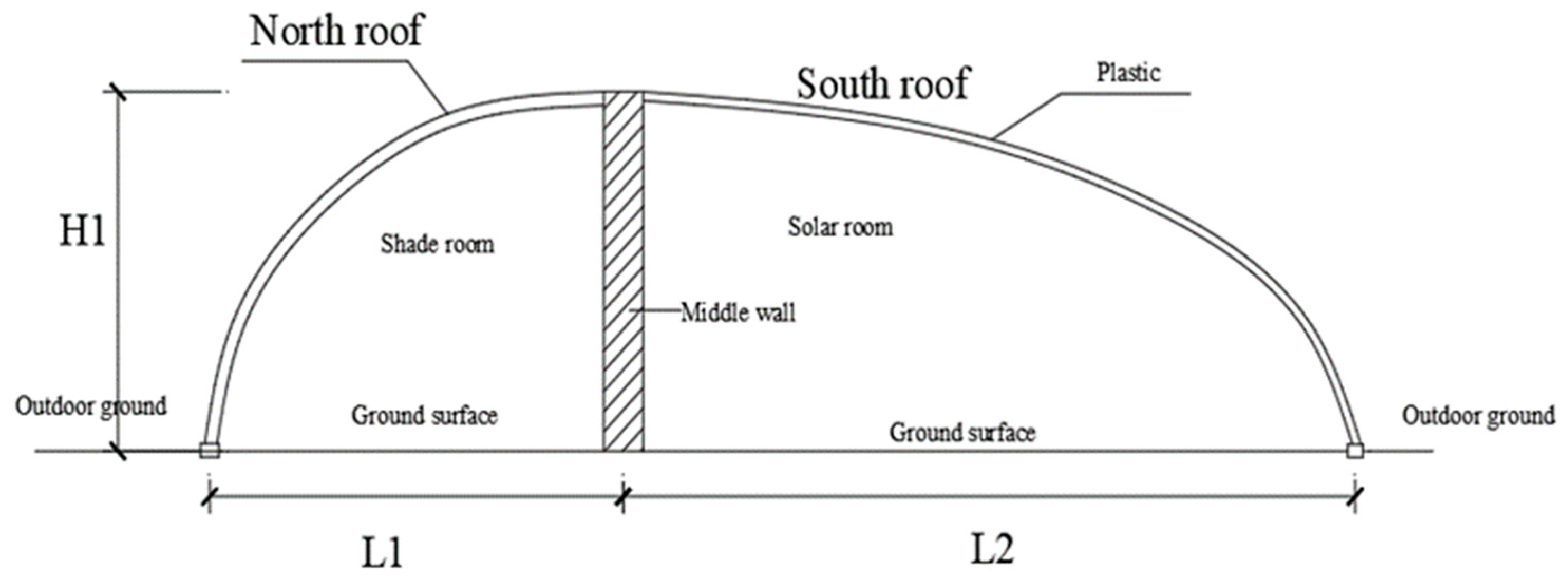
2.1. Greenhouse Parameter Setting

The Ecotect model of the experimental greenhouse was configured to match its actual dimensions and layout. Field measurements were conducted to assess light intensity at different locations within the greenhouse. These measured values were then compared and analyzed against simulated results generated by Ecotect. This comparative analysis aimed to evaluate and validate the accuracy and practicality of Ecotect software in replicating light distribution within the experimental greenhouse.

2.1.1. Test Greenhouse Parameters

The test greenhouse, located in Yantai City, Shandong Province, covers a total area of 100 m² with dimensions of 10 m in length, 10 m in width, and 3 m in height. It features a rear wall height of 2.1 m and has been designed with the solar room facing south and the shade room facing north. The greenhouse walls have been constructed using 240 mm thick aerated concrete blocks. The rear roof of the solar room is covered with 0.2 m thick double-layered colorful plywood filled with rigid polyurethane foam, providing insulation. In contrast, the shade room roof consists of 0.12 m thick rigid polyurethane material. The front roof of the solar room is covered with PVC membrane. To ensure effective environmental control, vents have been installed on both walls of the greenhouse. These vents facilitate optimal conditions for conducting experimental research.

2.1.2. Selection of Simulated Greenhouse Conditions

Ecotect software facilitates the simulation and analysis of greenhouse light environments through physical models and meteorological data inputs. It offers user-friendly operation and generates clear visualizations of simulation results. This study specifically examined the impact of window width and spacing on the roof of a double-slope greenhouse shade room, analyzing their effects on indoor temperature and light distribution. The greenhouse model accurately represents the dimensions, orientation, and construction materials of its components, with the exception of variations in window size and spacing [15,16].

Meteorological data sourced from Onebuilding.org were employed, focusing on Yantai City’s geographical coordinates (36.69° N latitude, 121.18° E longitude). This study specifically examined the shade room of a double-slope greenhouse, typically utilized for cultivating low-light crops or edible fungi. Indoor humidity levels were maintained at 75%, which is considered optimal for the growth of edible fungi [17], while indoor wind speed was set at 0.2 m/s. Meteorological conditions were derived from average values recorded on the coldest days.

Figure 1 depicts the model profiles of the double-slope greenhouses created using Ecotect. In addressing winter thermal insulation concerns, the experimental greenhouse’s shade room roof primarily utilizes polyurethane material. Roof windows, each 400 mm wide and constructed from double-layered transparent glass, have been installed to provide natural lighting for the shade room. These windows are positioned with their upper parts 600 mm from the roof and their lower parts 300 mm above the ground to prevent rainwater ingress during cloudy and rainy weather.

Table 1. Thermal performance parameters of simulated greenhouse materials.

Material	Density/kg·m−3	Specific Heat Capacity /J·(kg·K)−1	Heat Storage Coefficient /W·(m2·K)−1	Thermal Conductivity /W·(m·K)−1	Absorption Rate
Slag brick	1700	1050	12.72	0.87	0.50
EVA film	950	2010	-	0.04	-
Polyurethane	35	1380	0.54	0.02	-
FRP board	1500	1260	9.26	0.40	-
Planting soil	1600	1010	9.45	0.76	0.80
Air Gap	1.3	1004	-	0.03	-
Glass Standard	2300	836	-	1.05	0.12

details the thermal performance parameters for each section of the simulated double-slope greenhouse while

Table 2. Main parameters of the simulated greenhouse model.

Component	Parameter	Greenhouse
Greenhouse characteristics	Azimuth angle	South 180°
	Length/m	80
	Height (H1)/m	4.0
	Width of shade room (L1)/m	5.0
	Width of solar room (L2)/m	9.0
Middle wall	Height/m	4.0
	Total thickness/m	0.24
	Material and construction	Slag bricks cemented with cement mortar
East and west wall	Height/m	Shown in Figure 1
	Total thickness/m	0.56
	Material and construction	Slag brick wall at the outermost layer; the thickness is 0.12 m.
		Polystyrene board in the middle layer; the thickness is 0.07 m.
		Slag brick wall at the innermost layer; the thickness is 0.37 m.
North roof (Control group)	Material and construction	The lower 1/3 of the shade roof is used for light and the rest is covered with insulation.
		The inner layer is EVA plastic; the thickness is 0.0001 m.
North roof (Experimental group)	Material and construction	FRP board at the innermost layer; the thickness is 0.0008 m. Rigid foamed polyurethane in the middle layer; the thickness is 0.12 m. Smearing the surface with 1:2.5 cement mortar plus crack resistant fiber; the thickness is 0.02 m. The windows are aluminum-framed double-glazed windows with a glass thickness of 0.006 m and an intermediate air layer thickness of 0.004 m.
South roof	Material and construction	EVA plastic at the innermost layer; the thickness is 0.0001 m.
Ground	Ground cover	Shade room ground covered by bricks
		Solar room ground covered by planting soil
Location	Latitude	36.69° N
	Longitude	121.18° E
Simulating dates	The winter day	31 December

provides descriptions and dimensions of model components such as length, walls, and flooring [18].

• Modeling of sky brightness distribution

The purpose of sky brightness distribution modeling is to establish a foundational framework for leveraging solar energy. To effectively design and study natural lighting, a suitable sky brightness distribution model is essential. Over the years, researchers have developed various specific models for sky brightness distribution. The CIE standard cloudy sky model, derived from Moon and Spencer’s original model, simplifies the complexity of sky conditions. This standard model is commonly employed for calculating indoor lighting coefficients and assessing compliance with illumination standards [19]. When using Ecotect software to analyze illuminance in double-slope greenhouses, employing the full cloudy sky model ensures simulation accuracy while optimizing computation time and resources.

In the cloudy sky model, the brightness of any point M in the sky can be calculated by the following formula:

$${\displaystyle \frac{L_{\gamma }}{L_Z}}={\displaystyle \frac{1+\mathit{sin}\gamma }{3}}={\displaystyle \frac{1+\mathit{cos}Z}{3}}$$

(1)

Here,

• $L_{\gamma }$ is the zenith luminance value.
• $L_Z$ is the luminance value of any point in the sky.
• $\gamma$ is the altitude angle of point M.
• $Z$ is the angular distance degree between point M and the zenith.

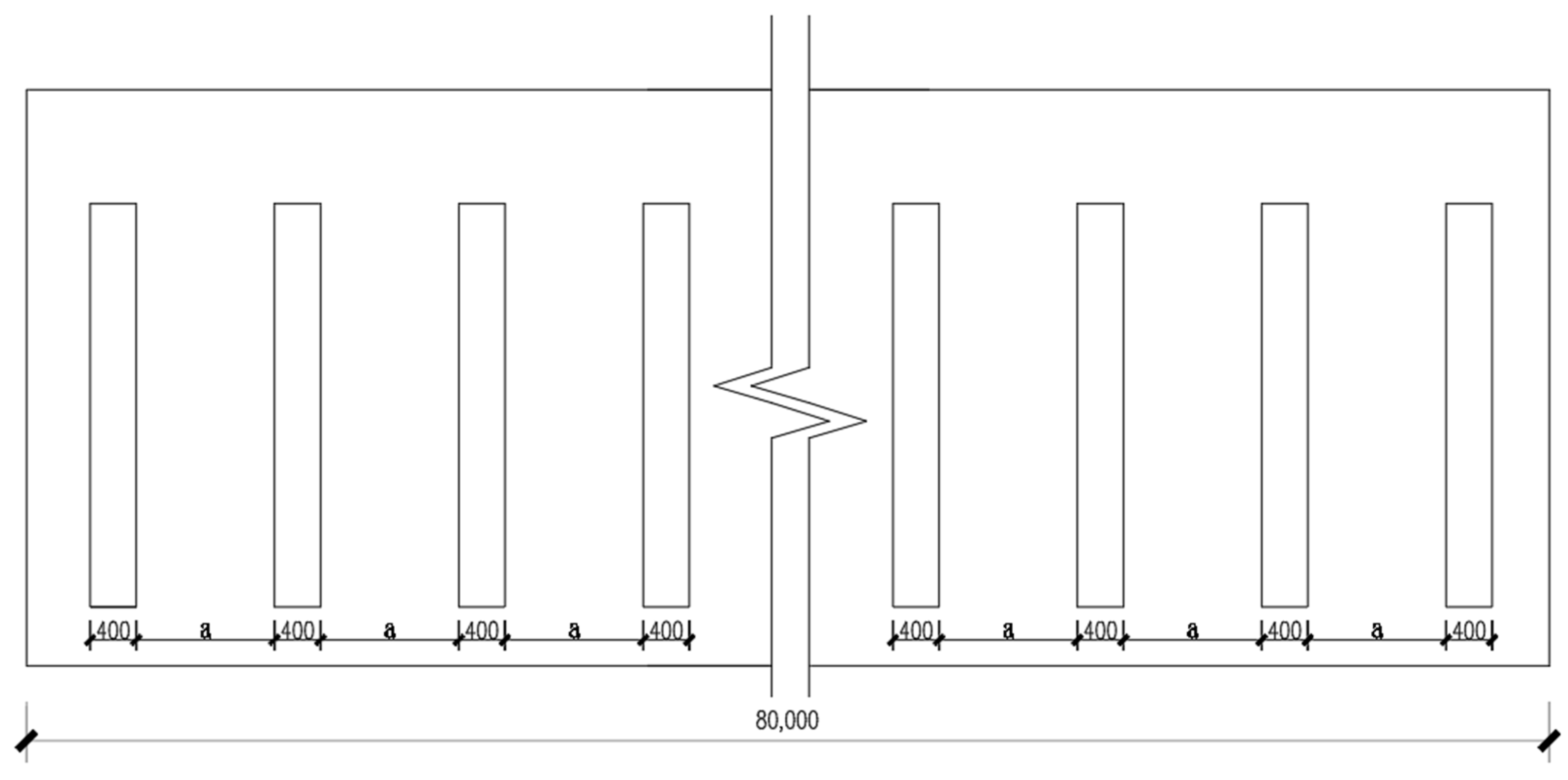
• Shade room roof window spacing settings

After establishing boundary conditions for each greenhouse component material and constructing five models of double-slope greenhouses, the light environment within these structures was simulated based on meteorological conditions in Yantai City. It was determined that the optimal north-window-to-wall ratio for these buildings should range between 0.1 and 0.25. This range effectively balances factors such as building energy consumption, natural light utilization, and thermal comfort, thereby optimizing overall building performance [20]. Accordingly, after calculating the area of the shadow shed walls, a window width of 400 mm was selected for simulating the greenhouse windows. Window spacings of 1000 mm, 2000 mm, 3000 mm, and 4000 mm were then chosen sequentially for double-slope greenhouses A, B, C, and D. In comparison with traditional double-slope greenhouse shed roof designs, which feature an inner layer of EVA plastic film and an outer layer of insulating cover, with 1/3 of the roof area left uncovered for daytime lighting, the simulated models of each greenhouse are illustrated in Figure 2. The design of the roof windows for the shade room is depicted in the top view shown in Figure 3. The spacing settings for the shade room windows are detailed in

Table 3. Spacing settings for the shade room windows in each greenhouse.

Components	Control Group	Greenhouse A	Greenhouse B	Greenhouse C	Greenhouse D
Window spacing(a)/mm	-	1000	2000	3000	4000

.

• Shade room roof window width setting

After conducting simulation analyses to determine the optimal window spacing, different window widths were set to explore the internal light environment of the shade room under varied roof window configurations. Taking into account factors such as construction cost, structural safety, and the north-window-to-wall ratio [20], window spacings of 300 mm, 400 mm, and 500 mm were sequentially selected for double-slope greenhouses A, B, C, and D, with all other conditions held constant.

2.1.3. Greenhouse-Equivalent Scale Model Parameters

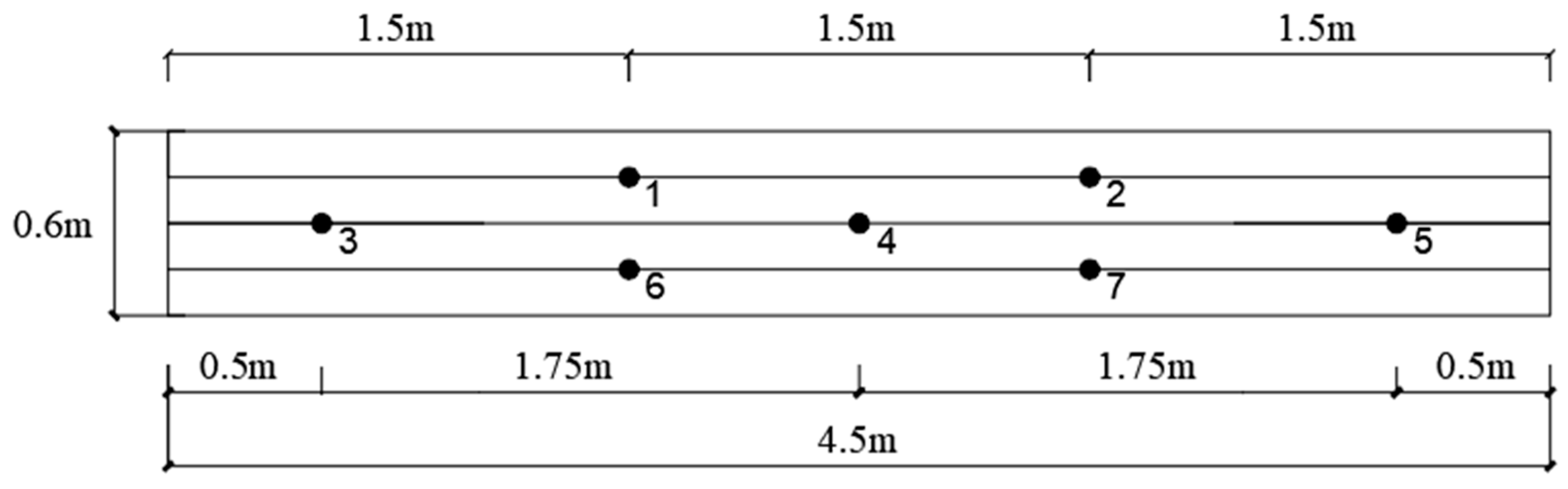
To investigate the impact of varying roller shutter openings and new shade room roofs on the light environments within double-slope greenhouse shade rooms, an equal-scale 1:8 model of the greenhouse was constructed, as depicted in Figure 4. The scaled model measured 4.5 m in length and 0.5 m in height, with a span of 1.2 m for the solar room and 0.6 m for the shade room. The frame of the model was constructed using density board and plywood. The roof of the solar room was covered with EVA transparent film while the shade room roof was made of plywood, incorporating long holes to simulate light transmission through the shade room roof. Due to the south-facing orientation of the greenhouse glazing, most of the interior areas, except for those near the east and west gables, experience a relatively uniform light environment along the length direction. Therefore, the impact of greenhouse length on the internal light environment can be considered negligible. Considering the constraints of the experimental conditions, the constructed greenhouse model approximates a 1:8 ratio in terms of span and height, though this ratio is not maintained along the length direction.

2.2. Test Methods

2.2.1. Software Validation

The actual greenhouse used in the testing, along with the Ecotect model of the greenhouse, was employed to demonstrate the efficacy of the simulation software. Given the substantial investment required to construct a greenhouse of the same dimensions as the simulated model, an alternative approach involves using an existing real greenhouse for modeling and simulation, complemented by field measurements. The dimensions of the real greenhouse have a minimal impact on the internal light conditions and can provide a reasonable reflection of the shading structure’s temperature. Therefore, comparing field measurements with simulation data serves as a valid method to validate the effectiveness of Ecotect. As illustrated in Figure 5, this experiment established three transects running in the east–west direction within the double-slope greenhouse shade room: east, center, and west. These transects were positioned 2 m from the east wall, at the middle of the greenhouse, and 2 m from the west wall, respectively. Along each transect, five measurement points were designated at intervals of 0.5 m, starting from 0.5 m to 4.5 m from the back wall, at a height of 1 m from the ground, the measurement points are numbered from 1 to 15. To evaluate the accuracy of the model, comparative analyses were conducted between measured light intensity data within the greenhouse and simulation results from Ecotect software at 12:00 on 22 December 2023. This specific time was selected due to its stable solar radiation conditions, facilitating reliable model analysis. Each measurement session was strictly controlled within a 5 min interval to ensure the accuracy and validity of the collected data.

2.2.2. Shade Room Light and Thermal Environment Simulation

• Simulation assessment of shade room light environment

In the light environment simulation, the numerical method employed is the radiative transfer method for illumination modeling, which is used to calculate the light distribution within the greenhouse. The simulation utilizes numerical solutions to the radiative transfer equation, including methods such as ray tracing and radiosity, to model how light propagates through space and interacts with objects within the greenhouse. For daylighting and lighting analysis, the simulated greenhouse is discretized into a grid with 80, 14, and 16 cells along the X, Y, and Z axes, respectively. The ray tracing accuracy is set to high value, with 4096 sampling points for the hemispherical light rays [21]. The window cleanliness is set to 0.9, and the CIE overcast sky luminance distribution model is used for the light simulation within the greenhouse. Since cash crops grown in greenhouses typically range in height from 0.5 m to 1.5 m above the ground, this experiment simulated light harvesting across the greenhouse cross-section at a height of 1 m from the ground. It analyzed the solar radiation illuminance received by each double-slope greenhouse at this specific height. After ensuring that the boundary conditions are appropriately set and reflect real-world scenarios, the greenhouse model is discretized into a grid and subjected to simulation analysis. Increasing grid density can enhance precision and reduce instability; however, an excessive number of grids significantly increases computational effort while having too few grids can compromise simulation accuracy. Therefore, selecting an appropriate grid size is crucial. In this study, a grid step size of 1 m was chosen, balancing computational efficiency with the accuracy requirements of the simulation. The simulated greenhouses, featuring varying window widths and window spacings, were assessed for light using Ecotect. The simulation results provided data on the light harvesting coefficient (%) and light harvesting illuminance (lux) [22,23].

The lighting coefficient at a point indoors is determined by the ratio of the illuminance received at that point, from the assumed and known sky luminance distribution, to the illuminance generated by the sky’s diffuse light on an unobstructed horizontal surface outdoors under the same sky conditions [24,25]. The formula for calculating the lighting coefficient $C$ is given as follows:

$$C={\displaystyle \frac{E_a}{E_b}}\times 100\%$$

(2)

Here,

• $E_a$ is the illuminance at the point indoors, received from the sky luminance distribution.
• $E_b$ is the illuminance on an unobstructed horizontal surface outdoors, generated by the sky’s diffuse light.

The illuminance at a point within a greenhouse is predominantly influenced by direct sunlight, scattered light from the sky, outdoor reflected light, and indoor reflected light. Analyzing and calculating the illuminance at a specific point indoors involves integrating contributions from these four sources. Here is the model for calculating the illuminance at a point within the greenhouse:

$$E_{total}=E_n+E+L_{wm}+E_r$$

(3)

Here,

• $E_n$ is the illuminance produced by direct sunlight at the point.
• $E$ is the illuminance of the point subjected to scattered light from the sky.
• $L_{wm}$ is the illuminance of the point that receives reflected light from outdoors.
• $E_r$ is the illuminance produced by reflected light from indoors.

The specific calculations for each component are as follows.

The illuminance produced by direct sunlight at the interior spot is calculated by Equation (4):

$$En=E_S\times \tau \times {\tau }_C\times {\tau }_w$$

(4)

Here,

• $E_S$ is the light intensity produced by direct sunlight on the horizontal outdoor surface.
• $\tau$ is the visible light transmittance of the glass.
• ${\tau }_C$ is the light-blocking discount factor of the window structure.
• ${\tau }_w$ is the pollution discount factor of the glass.

The illuminance level at a point in a room due to scattered light from the sky primarily depends on the brightness of the sky visible through windows at that point. On cloudy days, the illuminance near windows is typically higher than in deeper parts of the room because the sky area visible near windows is larger compared to deeper areas. As you move deeper into the room away from windows, the illuminance level gradually decreases.

The illuminance of a point in the room generated by the scattered light from the sky can be calculated by the law of stereographic projection. Assuming that the P surface has the same brightness in all directions of the light-emitting surface, Q is an indoor illuminated surface. In the P surface’s selected micro element area $dP$, the horizontal illuminance generated at a point O on the surface Q is given as follows:

$$dE=L_{\alpha }d\Omega \mathit{cos}i$$

(5)

Here,

• $L_{\alpha }$ is the value of the surface brightness of the P plane.
• $\Omega$ is the stereo angle of the O point with respect to the micrometric plane $dP$.
• $i$ is the angle between the normal of the plane Q and the micrometric plane $dP$.

Then, the illuminance level produced by the entire luminous surface P at point O is as follows:

$$E=\underset{\Omega }{\int }{L}_{\alpha }d\Omega \mathit{cos}i$$

(6)

When the light source surface is equally bright in all respects,

$$dE=L_{\alpha }\Omega \mathit{cos}i.$$

(7)

Calculating the illuminance indoors due to outdoor reflected light is complex due to the variability of outdoor conditions. However, the light entering a room from outdoor reflections and scattered sky light generally follows similar principles, making it feasible to use the law of three-dimensional angular projection. This law allows us to compute the illuminance on an indoor horizontal surface generated by the surface brightness of the outdoor environment at a specific point. Here is how the surface brightness $L_{wm}$ of each outdoor environment, approximated as a uniform diffuse reflective surface, can be calculated:

$$L_{wm}={\displaystyle \frac{E_{wm}\times \rho }{\pi }}$$

(8)

Here,

• $E_{wm}$ is the surface illuminance of the outdoor environment.
• $\rho$ is the visible light reflectance of the surface of the outdoor environment.

For the calculation of illuminance generated by reflected light at a point in the room, the “luminous flux decomposition method” recommended by the Institute of Building Research of the United Kingdom can be used. It divides the window light flux decomposition into two parts: downward light flux ${\varphi }_{FW}$-irradiation to the window center plane below the wall and the ground light flux and upward light flux ${\varphi }_{CW}$-irradiation to the window center plane above the wall and the roof of the light flux. Then, at this point, the illuminance produced by the reflected light in the room at a certain point can be expressed as follows:

$$E_r\left[lm/unit-area\right]={\displaystyle \frac{{\varphi }_{FW}{\rho }_{FW}+{\varphi }_{CW}{\rho }_{CW}}{A\left(1-\rho \right)}}$$

(9)

Here,

• ${\rho }_{FW}$ is the average reflection coefficient per unit area of the floor and walls below the center plane of the windows.
• ${\rho }_{CW}$ is the average reflection coefficient per unit area of the roof and walls above the center plane of the windows.
• $A$ is the total internal surface area of the greenhouse.
• $\rho$ is the average reflection coefficient per unit area of the internal surface.

Solar radiation is transmitted through the greenhouse roof at various locations inside the greenhouse due to the fact that angle of incidence of light and the transmittance of roofing materials are not the same at each location, resulting in differences in the intensity of solar radiation in the horizontal and vertical directions of the greenhouse. The uniformity of light distribution (%) evaluates the uniformity of light distribution in the greenhouse and indirectly reflects the utilization of solar radiation energy by crops in the greenhouse.

Light distribution uniformity calculation formula is as follows:

$$\rho =1-{\displaystyle \frac{\left(\sqrt{\frac{\sum _{j=1}^n{\left(I_j-I_m\right)}^2}{\left(n-1\right)}}\right)}{I_m}}$$

(10)

Here,

• $\rho$ is the uniformity of light distribution.
• $n$ is the number of measurement points.
• $I_j$ is the light intensity (lux) of the $j$th measurement point.
• $I_m$ is the average value of indoor light intensity (lux).

To enhance the thermal insulation performance of the double-slope greenhouse, the windows in the simulated greenhouse are all equipped with double-glazed transparent glass. The formula for calculating the spectral transmittance of the double-glazed window unit is as follows:

$$\tau \left(\lambda \right)={\displaystyle \frac{{\tau }_1\left(\lambda \right){\tau }_2\left(\lambda \right)}{1-{\rho }_1^{\prime }\left(\lambda \right){\rho }_2\left(\lambda \right)}}$$

(11)

Here,

• $\tau \left(\lambda \right)$ is spectral transmittance of the exterior side of the double-glazed window unit.
• $\lambda$ is wavelength.
• ${\tau }_1\left(\lambda \right)$ is spectral transmittance of the first layer of glass.
• ${\tau }_2\left(\lambda \right)$ is spectral transmittance of the second layer of glass.
• ${\rho }_1^{\prime }\left(\lambda \right)$ is spectral reflectance of the first layer of glass when light is incident from the interior side to the exterior side.
• ${\rho }_2\left(\lambda \right)$ is spectral reflectance of the second layer of glass when light is incident from the exterior side to the interior side.

• Simulation assessment of shade room thermal environment

Ecotect was employed to simulate and analyze the internal temperatures of shade rooms under varying window widths, aiming to assess whether the simulated conditions could meet the growth requirements of edible mushrooms. In the thermal environment simulation, a heat conduction model is employed to simulate heat transfer and temperature distribution within the greenhouse. The finite element method is utilized to solve the partial differential equations associated with heat conduction. Meteorological data from Yantai City were imported into Ecotect using the Weather Tool, with the date set as 31 December 2023. This setup simulated the internal temperature of the shade room under different operational scenarios aligned with Yantai City’s weather conditions for that specific day. Temperature curves were generated over time to depict the internal temperature variations in each greenhouse.

2.2.3. Validation Test Methods

The XM8562 bracket-type light sensor, manufactured by Shanghai XUNCHIP Technology Company (Shanghai, China), has been specifically engineered for monitoring light intensity in optical instruments. It features a high-precision sensing core and accompanying components that guarantee both reliability and long-term stability. The sensor boasts a wide light measurement range of 0–65,535 lux with a maximum allowable error of ±7%. Importantly, it is designed to measure light across wavelengths ranging from 380 nm to 730 nm, covering the visible spectrum comprehensively. This capability ensures versatile and accurate light measurement in various applications within this wavelength range.

The XM8562 bracket-type illuminance sensor was used to measure light intensity in the shade room under different conditions by arranging 7 measurement points uniformly inside the shade room of the double-slope greenhouse model. The primary objective of this validation experiment was to test the uniformity of light distribution on the same plane inside different roof shading canopies. This aimed to investigate the uniformity of light distribution on the cultivation beds for edible mushrooms within the greenhouse during actual production processes. Since the placement of the light radiation sensors only affected the received light intensity, it was sufficient for the sensors to be uniformly distributed within the shade room. The test location was indoors in Yantai City, Shandong Province, and the test occurred on 22 April 2024, during sunny weather with outdoor light intensity at 18,652 lux. The arrangement of measurement points inside the shade room is shown in Figure 6 and the actual setup and interface of the light intensity monitoring are depicted in Figure 7, in Figure 6, numbers 1–6 indicate the precise locations of the sensor placement points. Corresponding to Figure 6, Figure 7 shows the actual positions of the monitors. The XM8562 sensor facilitated the measurement of light intensity in the shade room of the double-slope greenhouse model. Through the actual measurement of light intensity and the evaluation of light distribution uniformity inside the greenhouse under new roof conditions and different roller shutter openings, the study verified the effectiveness of the new roof in improving the light environment of the shade room.

3. Results and Discussion

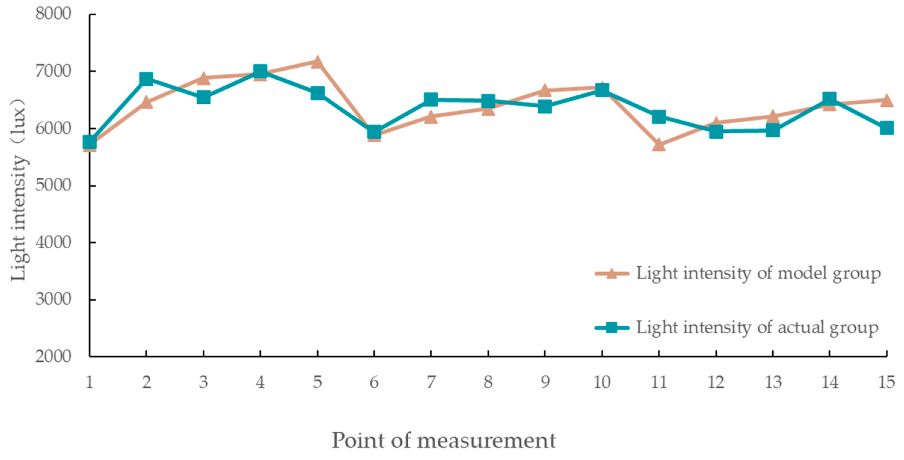
3.1. Results of Validation of the Effectiveness of the Simulation Software

Figure 8 shows a relatively uniform light intensity distribution within the greenhouse, maintaining stability between 6000 and 7000 lux at noon. Due to differences in test sky conditions, simulation data and test measurements at the same points varied, but the overall trends were consistent. Generally, the south side of the greenhouse exhibited higher light intensity compared to the north, and the west side was better illuminated than the east. The maximum error between test and simulated data was 8.3%, the minimum error was 1.2%, and all errors were within 10%, confirming the accuracy of the model and the effectiveness of using Ecotect software for simulation purposes. During the actual testing process, it was observed that the east gable caused shading in the nearby areas, resulting in lower light intensity compared to other regions. The simulation also accounted for the shading effect of the gables. The results indicated that both the simulated and measured data showed a slight reduction in light intensity near the east gable, with discrepancies between the two being within 10%.

3.2. Analysis of Shade Room Light and Heat Environments

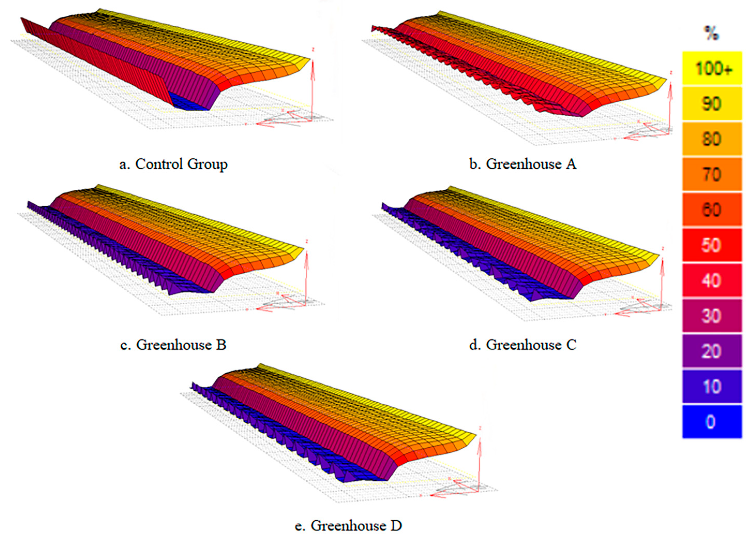
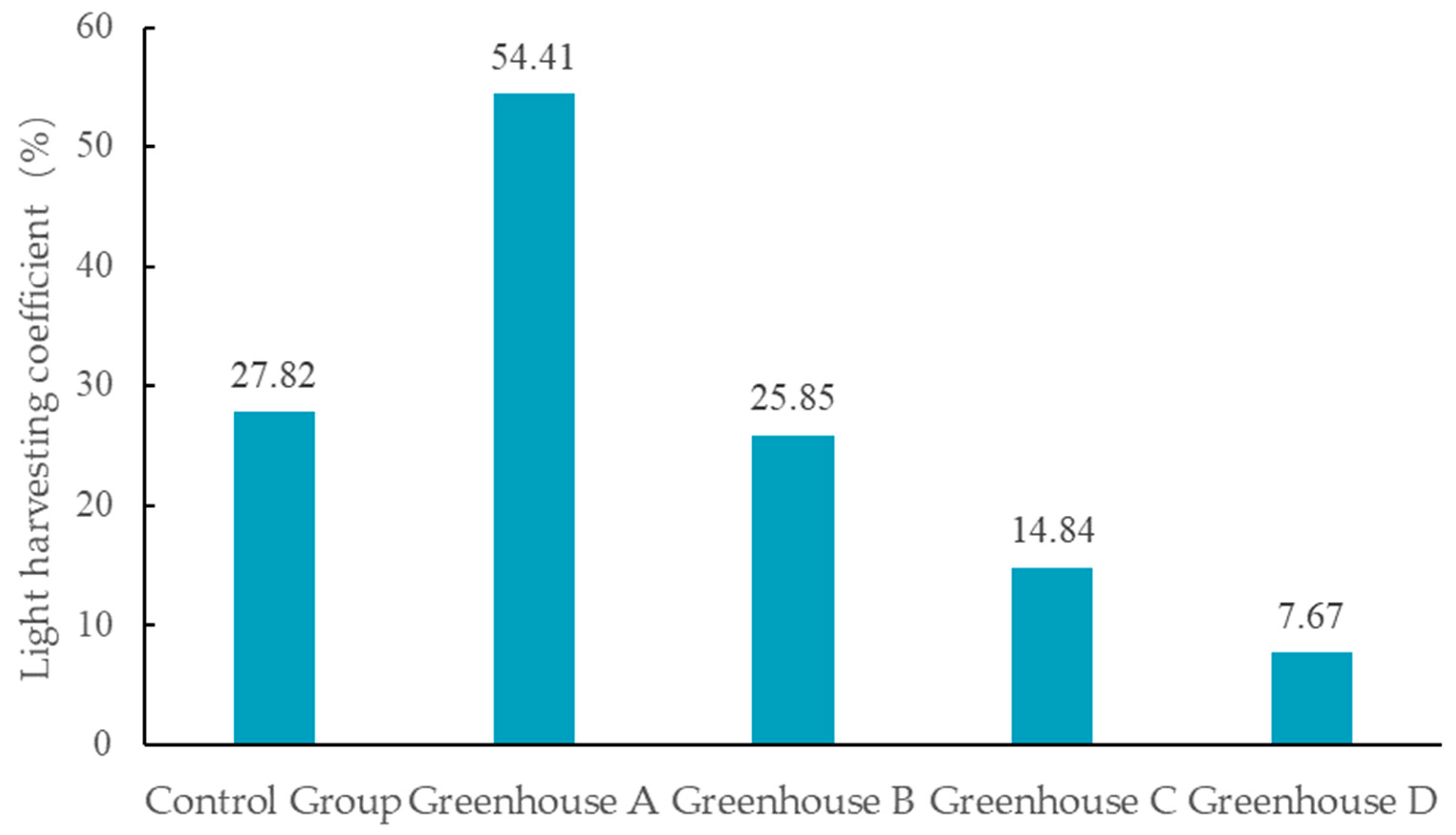
3.2.1. Analysis of Shade Room Light Environment with Different Window Spacings

Figure 9 depicts the lighting coefficient contour map of the double-slope greenhouse at 1 m above the ground under five different window spacings [26,27]. The contour ranges from 0% to 100% in 10% increments, with blue indicating the lowest lighting coefficient and yellow indicating the highest. The ground lighting coefficient in the shade room showed a general decrease from north to south across the greenhouse. The windows, being the sole natural lighting source in the shade room, significantly improved the lighting coefficient. Due to shading from the gable walls on the east and west sides, the light transmission coefficient in the areas near these gables showed a notable decrease, as depicted by the concave shape in Figure 9. The average light transmission coefficient was lowest at the corners of the rear wall, where the combined shading effects of the rear wall and the side gables were most pronounced.

As depicted in Figure 10, double-slope greenhouse D exhibited the lowest average light harvesting coefficient among all simulated greenhouses at 7.67%. This was attributed to the fact that all light entering the shade room of this experimental greenhouse came through areas of the roof not covered by an insulating blanket, resulting in significantly higher light transmission near the roof’s translucent sections compared to other indoor locations. Among the simulated greenhouses, double-slope greenhouse A featured the largest window area, allowing the highest amount of light transmission into the shade room. Consequently, it achieved the highest average light harvesting coefficient of 54.41%, which was notably superior to those of the other greenhouse designs.

Figure 11 displays the illuminance distribution of five double-slope greenhouses at a height of 1 m from the ground. The illuminance distribution map has a step size of 800 lux, ranging from 0 to 8000 lux. The map shows a gradual decrease in natural lighting illuminance from north to south within the shade rooms of the double-slope greenhouses, with the lowest illuminance observed at the east and west corners of the back wall. Figure 12 presents the average natural light illuminance values for the shade rooms of the five double-slope greenhouses. The control greenhouse exhibited very high illuminance near the translucent areas, exceeding 5500 lux. However, in areas not directly exposed to sunlight, particularly in the shade room without direct sunlight to the south, illuminance ranged only from 200 to 400 lux; however, the light intensity in areas exposed to direct sunlight was consistently above 4800 lux, indicating uneven light distribution. Among the greenhouses, double-slope greenhouse A, with the largest window area receiving direct sunlight, achieved significantly higher internal illuminance compared to others, reaching 2928.2 lux. In contrast, double-slope greenhouse D, with the smallest window area and minimal direct sunlight penetration, relied mainly on diffuse light, resulting in the lowest natural light illuminance at 442.6 lux.

Figure 13 illustrates the uniformity of light distribution in each simulated greenhouse shade room, showing higher uniformity at noon compared to the morning and evening. Greenhouse A exhibited superior light distribution uniformity among all the greenhouses, achieving 75.2% uniformity at noon. This was attributed to the direct vertical sunlight irradiation of the shade room at noon, ensuring the north-facing windows received the most evenly distributed light. In contrast, the control greenhouse showed the poorest light distribution uniformity. Light was concentrated in the north side of the shade room where there was no thermal insulation blocking, resulting in rapid decreases in light intensity from north to south. Throughout the day, the uniformity of light distribution remained lower compared to other greenhouses, with a peak of only 39.8% at noon. Morning and evening periods saw uneven light distribution due to obstruction by the east and west walls and the back wall. Due to the north–south orientation of the double-slope greenhouse, sunlight was primarily blocked by the back wall at around noon. The projection of sunlight rays was nearly perpendicular to the back wall, resulting in the highest uniformity of light distribution in the shade room during midday with minimal variation. Overall, greenhouse A demonstrated the highest uniformity of light distribution and the most efficient utilization of light energy for crops grown inside.

Comparing the lighting performances of the five double-slope greenhouses with different shade room roof structures, the findings highlight significant differences in the lighting coefficient and illuminance. Greenhouse A, featuring a window spacing of 1000 mm, exhibited a notably higher lighting coefficient and illuminance compared to the other designs, indicating superior lighting performance. However, the intense direct light could potentially inhibit the growth of edible fungi and even cause harm. Conversely, simulated greenhouse D showed insufficient and uneven light distribution, rendering it unsuitable for the growth of edible fungi. Greenhouse C demonstrated moderate internal light intensity, with relatively uniform light distribution across all simulated greenhouses. Thus, it can be concluded that a window spacing of 3000 mm provides the best balance between light intensity and distribution for creating a suitable environment for the growth and development of edible fungi.

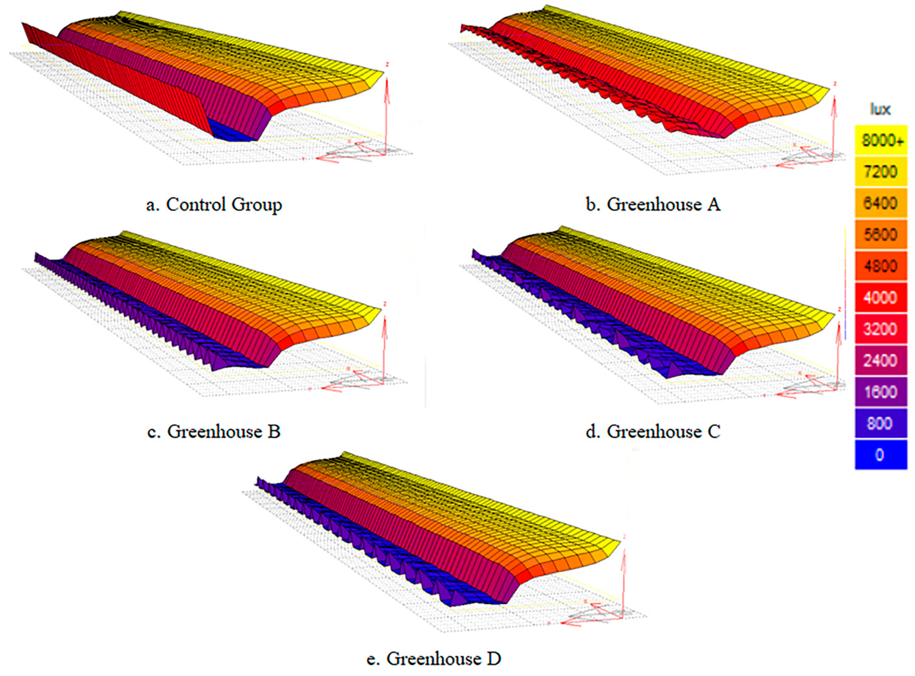
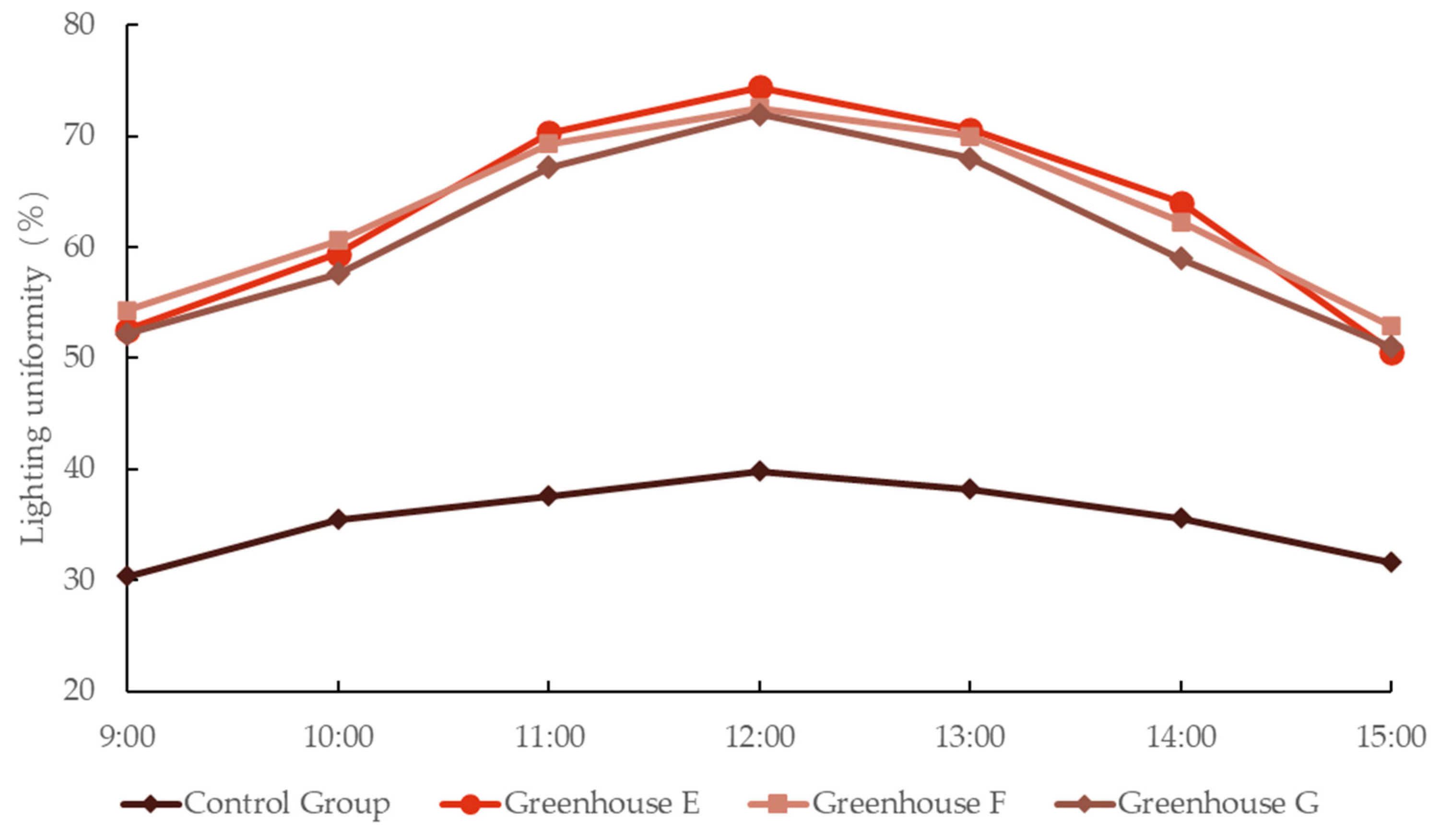
3.2.2. Analysis of Shade Room Light Environment with Different Window Widths

After determining the 3000 mm pitch as optimal for the shade room roof, we proceeded with Ecotect to establish double-slope greenhouse models featuring different shade window widths. We conducted simulations to calculate light distribution uniformity as shown in Figure 14. Figure 14 illustrates that light distribution uniformity in the three experimental greenhouses was lower at 9:00, characterized by stronger sunlight on the east side due to the sun’s positioning. As the sun moved south from 9:00 to 12:00, light intensity gradually became more vertical, enhancing uniformity inside the shade room. Post-noon, sunlight shifted towards the west, intensifying on that side and reducing uniformity [28]. Overall, light distribution uniformity inside the shade room with varying window widths showed minimal differences. The double-slope greenhouse with a 300 mm window width exhibited slightly superior performance, achieving the highest uniformity of 74.4% at 12:00 p.m. This indicated the most even light distribution, optimal light environment, and highest light energy utilization by the crops inside the shade room.

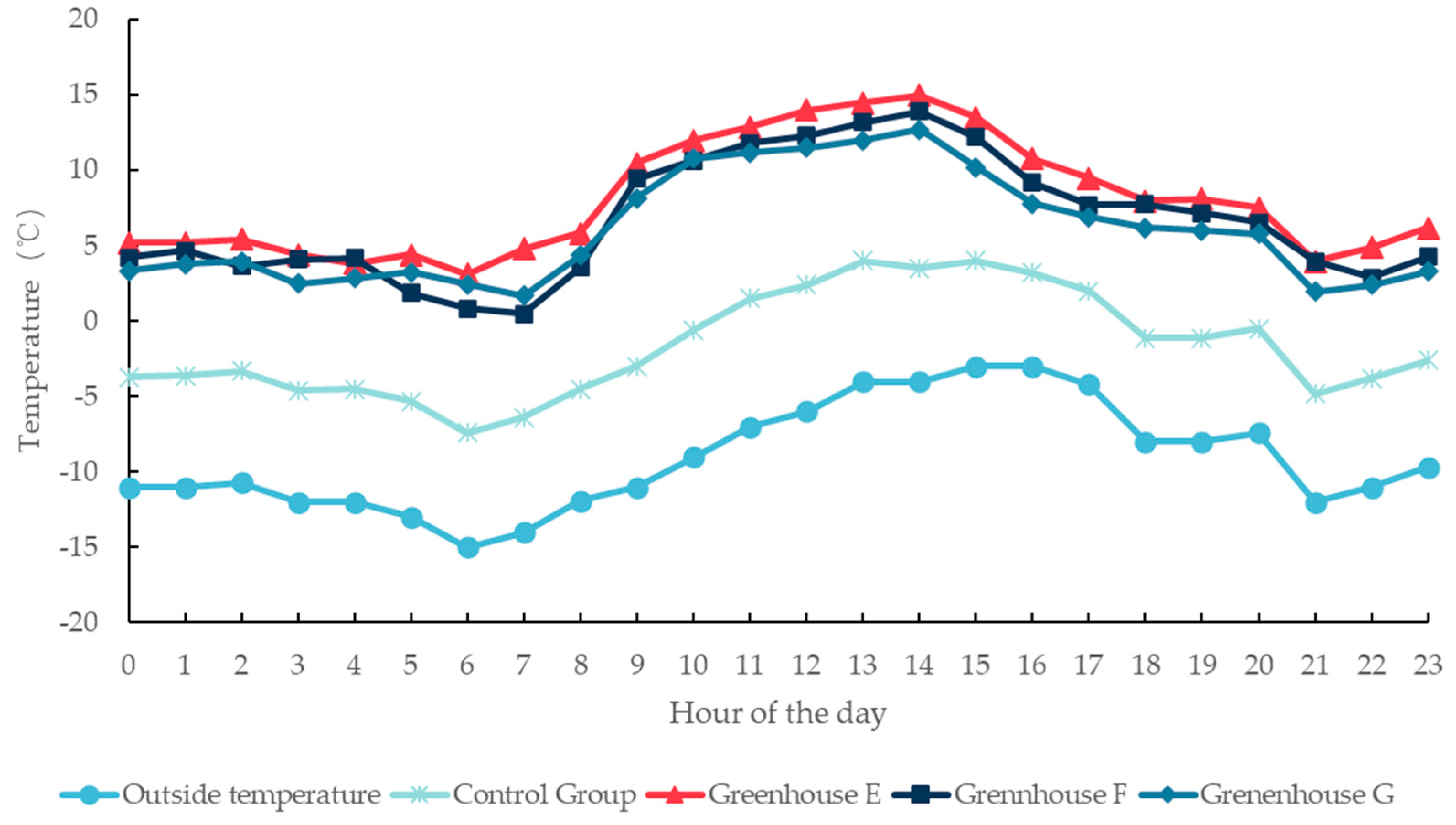
3.2.3. Analysis of Shade Room Heat Environment with Different Window Widths

The hour-by-hour graphs of air temperature in the shade room of each greenhouse are shown in Figure 15 [29].

Figure 15 illustrates the hourly internal temperature variations of the shade rooms in three experimental greenhouses compared to the control greenhouse on 31 December. The experimental greenhouses benefited from enhanced solar radiation due to their roof window designs, resulting in more uniform light distribution. Consequently, the temperature inside these shade rooms increased with solar intensity, significantly surpassing that of the control group. At night, the polyurethane roofing effectively insulated the experimental shade rooms, maintaining higher indoor temperatures. Notably, double-slope greenhouse E exhibited the most favorable temperature conditions, reaching a daytime high 15.0–11.5 °C higher than the control greenhouse—and nighttime temperatures 8.1–9.0 °C higher than the control group.

The simulation results indicated that implementing a new shade room roof design can enhance the indoor temperature environment of double-slope solar greenhouse shade rooms to a certain extent. However, during winter nights, heat exchange between the warm indoor air and cold outdoor air through the windows results in lower indoor temperatures in the shade room, which may not be suitable for the growth of edible fungi. Therefore, alongside the new roof design, it is crucial to prevent heat exchange by covering insulation quilts over the windows at night. This dual approach will improve the indoor light environment and raise the shade room’s winter temperatures, optimizing conditions for the growth of crops, particularly edible fungi.

Based on the above analysis, the optimal design of the new shade room was chosen to have a window spacing of 3000 mm and a window width of 300 mm.

3.3. Verification Test Result Analysis

The results of the verification test experiment are presented in

Table 4. Illuminance intensity and uniformity inside the greenhouse shade room under different curtain openings and new roof types.

Curtain Opening	Average Illumination Intensity/(lux)	Illumination Distribution Uniformity/(%)
0°	-	-
30°	395	53
60°	582	78
90°	686	93
Designed new roof	325	92

; the average light intensity is the mean value of the light intensities measured at seven sampling points [30].

Because the illumination intensity testing was conducted indoors, the measured values were relatively lower compared to outdoor measurements. Therefore, this test primarily examined the uniformity of illumination distribution within the greenhouse shade room under different conditions. As shown in Table 4, with the curtain opening at 30°, the illumination distribution inside the shade room was poor at only 53.1% uniformity. Uneven illumination can result in varied mushroom growth levels across different locations within a shade room, leading to differences in quality within the same production batch. When the curtain opening increased to 60° and 90°, the illumination distribution became relatively uniform. However, a larger area of light transmission can cause significant heat loss within the shade room, resulting in excessively low temperatures that inhibit mushroom growth and reduce production yields. With the implementation of the new roof type, the illumination distribution within the shade room became more uniform, with moderate illumination intensity that met the growth requirements of mushrooms without adverse effects.

Using MATLAB R2022b software, the illumination intensity analysis of the shade room with a curtain opening at 30° and the shade room using the new roof type were conducted. The results are shown in Figure 16.

As shown in Figure 16a, there was a noticeable stratification in the illumination intensity distribution within the shade room with a curtain opening at 30°. The illumination was concentrated near the translucent area on the ground, with the lowest illumination intensity observed at the rear wall. The uniformity of illumination within the shade room was poor. Figure 16b illustrates the illumination situation inside the shade room using the new roof design. It can be observed that the illumination distribution on the shade room floor was uniform, with illumination intensity ranging from 300 to 400 lux, indicating an ideal testing outcome.

As shown in Figure 16a, in the shade shed with a curtain opening angle of 30°, a significant stratification of light intensity distribution was observed. Light was concentrated near the translucent area of the ground, where direct sunlight reached intensities exceeding 600 lux. The light intensity was lowest in the middle of the rear wall, measuring less than 200 lux. This indicated the poor uniformity of the light environment inside the shed at this configuration. Figure 16b illustrates the light conditions inside the shade shed using the new roof design. It is evident that the light intensity on the ground remained within the range of 300–400 lux, with no significant shadowed areas observed. The distribution of light on the shade shed floor was uniform, indicating an ideal testing outcome.

4. Conclusions

Aiming at the problem of poor light environments in double-slope greenhouse shade rooms, a new type of shade room roof was designed to provide a suitable light and heat environment for overwintering the production of crops in shade rooms. The main contributions were as follows:

(1)

The light simulation and field measurement of typical double-slope greenhouses in Yantai City were carried out and it was verified that the error between the simulated value of light intensity and the measured value was no more than 10%, which met the accuracy requirement, proving the effectiveness of Ecotect simulation in analyzing the light environments of greenhouses.

(2)

The simulation of the internal light and thermal environment in the shade shed under different window configurations indicated that a window spacing of 3000 mm was optimal. This configuration resulted in moderate light intensity and a noon sunlight uniformity of 72.6%, which represented a 42.8% improvement compared to a typical double-slope greenhouse. A window width of 300 mm was found to be optimal, achieving a sunlight uniformity 1.8% to 2.4% higher than other experimental greenhouses. The shade shed maintained a stable temperature above 5 °C, with an average temperature 1.4 °C to 2.1 °C higher than other experimental setups. The temperature differential with the outside environment reached up to 17.1 °C, indicating significant insulation efficiency.

(3)

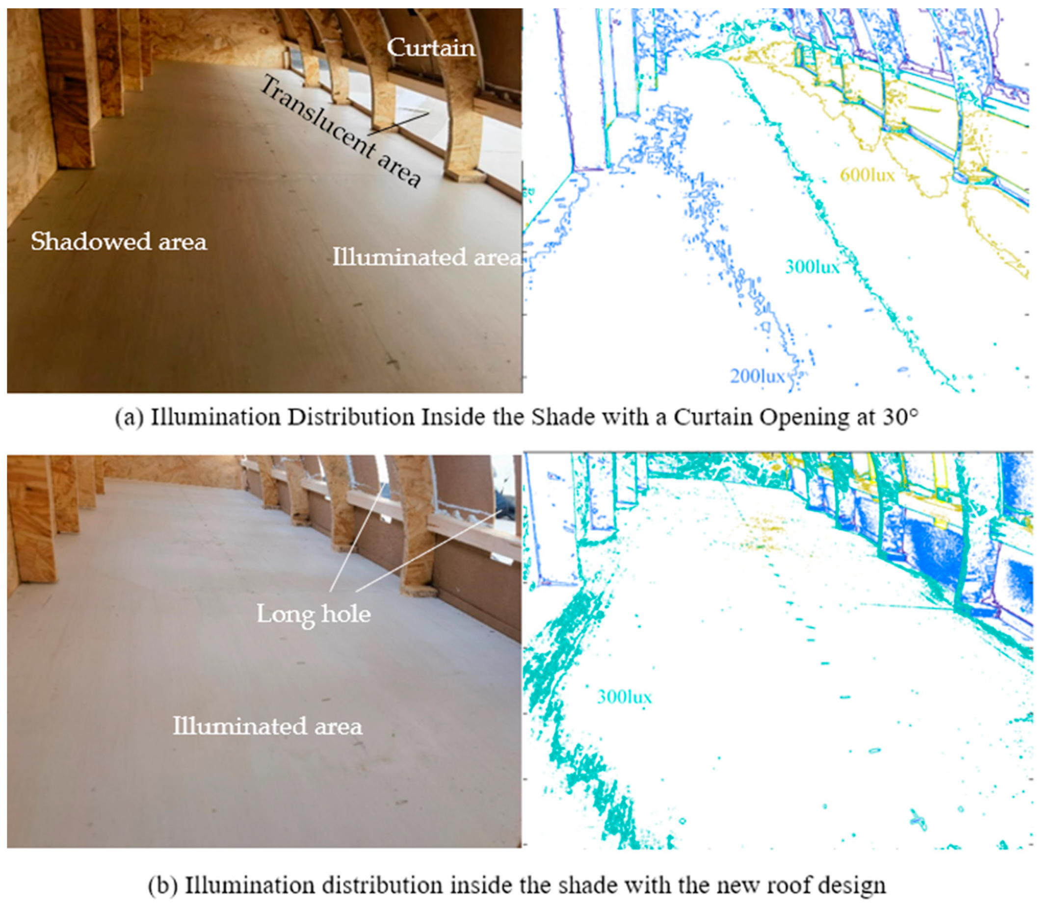
Simulation experiments indicated that increasing the area of roof windows in the shade room could improve the internal light environment. However, excessively large window areas could lead to significant heat loss, resulting in a reduction in internal temperatures, which is detrimental to crop growth; it could also increase the actual investment and operating costs of greenhouse production. Considering the above test results, taking into account the temperature, light environment, and construction costs required for the growth of edible fungi, one must choose the spacing of 3000 mm and width of 300 mm as the optimal design of the shade room roof windows. The designed new roof can effectively improve the uniformity of light in the shade room and improve the quality and consistency of mushroom production in the shade room. It provides a new idea for energy saving and consumption reduction for improving the winter light and heat environments of double-slope greenhouse shade rooms, realizes the efficient use of clean energy, and meets the requirements of the sustainable development of modern agriculture.

References

1. Chen, L. Design of semi-underground double-arch three-membrane Yin-Yang greenhouse. Tibet Sci. Technol. 2020, 1, 15–17. [Google Scholar]
2. Yu, Q.; An, X.; Wei, C.; Li, X. Analysis of temperature environment in Yin-Yang greenhouse. Anhui Agric. Sci. 2016, 44, 37–40. [Google Scholar]
3. Su, D.; Wang, T.; Li, M.; Meng, S. Planning and design of Yin-Yang combined greenhouse. J. Shenyang Agric. Univ. 2002, 2, 138–141. [Google Scholar]
4. Zhou, C.; Liu, C.; Wang, J. Preliminary exploration of environmental conditions in Yin-Yang type greenhouse. In Proceeding of the 2009 China Shouguang International Horticultural Forum, Shouguang, China, 20 April 2009; Volume 6, pp. 133–138. [Google Scholar]
5. Li, Y.; Yu, H.; Zhou, F.; Wang, R.; Li, Z.; Guo, Q. Research progress on the effect of light on the growth and development of edible fungi. Edible Fungi 2011, 33, 3–4. [Google Scholar]
6. Qian, L.; Zhang, Z.; Zhou, Y.; Liu, L.; Luo, Y.; Liu, J. Influence of light on the growth of edible fungi. Tianjin Agric. Sci. 2017, 23, 103–106. [Google Scholar]
7. Fan, C. Influence of light on the growth and development of Agaricus bisporus. Yunnan Plant Res. 1983, 2, 201–205. [Google Scholar]
8. Shi, W.; Liu, S.; Liu, S.; Yuan, H.; Ma, J.; Liu, H.; An, F. Analysis of the impact of artificial water diversion on the ecological environment of Qingtu Lake area downstream of Shiyang River. Acta Ecol. Sin. 2017, 37, 5951–5960. [Google Scholar]
9. Sher, F.; Kawai, A.; Güleç, F.; Sadiq, H. Sustainable energy saving alternatives in small buildings. Sustain. Energy Technol. Assess. 2019, 32, 92–99. [Google Scholar] [CrossRef]
10. Fang, Z.; Wang, X.; Huang, Q.; Pang, Z. Simulation and analysis of greenhouse environmental parameters based on Ecotect. Trop. Biol. 2016, 7, 99–103. [Google Scholar]
11. Wang, B.; Chen, J.; Ying, J. Analysis of photovoltaic greenhouse indoor light environment based on Ecotect. Jiangsu Agric. Sci. 2018, 46, 221–224. [Google Scholar]
12. Sun, Y.; Bao, E.; Zhu, C. Effects of window opening style on inside environment of solar greenhouse based on CFD simulation. Int. J. Agric. Biol. Eng. Assess. 2020, 13, 53–54. [Google Scholar] [CrossRef]
13. Inouea, T.; Ichinoseb, M. Advanced technologies for appropriate control of heat and light at windows. Energy Procedia. Assess. 2016, 96, 33–41. [Google Scholar] [CrossRef]
14. Yu, S.; Cui, Y.; Xu, X.; Feng, G. Impact of Civil Envelope on Energy Consumption Based on EnergyPlus. Procedia Eng. 2015, 121, 1528–1534. [Google Scholar] [CrossRef]
15. Yun, P. Ecotect Building Environmental Design Tutorial; China Architecture & Building Press: Beijing, China, 1994. [Google Scholar]
16. Bai, M. Autodesk Ecotect Analysis 2011 Green Building Analysis Examples; China Architecture & Building Press: Beijing, China, 2011. [Google Scholar]
17. Zhao, C.; Xie, F.; Wu, P. Research progress on the effects of environmental factors on the sexual development of edible fungi. Chin. Agric. Bull. 2014, 30, 87–92. [Google Scholar]
18. GB/T50176—2016; Code for Thermal Design of Civil Buildings. Ministry of Housing and Urban-Rural Development of the People’s Republic of China: Beijing, China, 2016.
19. Yu, L. Study on the Influence of External Shading on Indoor Light Environment in Buildings. Master’s Thesis, Chongqing University, Chongqing, China, 1 April 2010; p. 91. [Google Scholar]
20. Qin, W. Multi-Objective Optimization Research on High-Rise Residential Buildings in Cold Regions Based on Energy Consumption and Thermal Performance. Master’s Thesis, Inner Mongolia University of Technology, Mongolia, China, 2023; p. 41. [Google Scholar]
21. He, D.; Chang, J.; Xing, H. Direct Radiation Model of Louver Shading in Office Building Shade Based on Network Optimization Method. Comput. Intell. Neurosci. 2022, 2022, 5766448. [Google Scholar] [CrossRef]
22. Acosta, I.; Navarro, J.; Sendra, J.J. Towards an Analysis of Daylighting Simulation Software. Energies 2011, 4, 1010–1024. [Google Scholar] [CrossRef]
23. Xin, P.; Li, B.; Zhang, H.; Hu, J. Optimization and control of the light environment for greenhouse crop production. Sci. Rep. 2019, 9, 13–15. [Google Scholar] [CrossRef]
24. Lu, M.; Zhang, Y.; Xing, J.; Ma, W. Assessing the Solar Radiation Quantity of High-Rise Residential Areas in Typical Layout Patterns: A Case in North-East China. Buildings 2018, 8, 148. [Google Scholar] [CrossRef]
25. Kwon, C.; Lee, K. Integrated Daylighting Design by Combining Passive Method with DaySim in a Classroom. Energies 2018, 11, 3186. [Google Scholar] [CrossRef]
26. Varoğlu, S.E.; Altın, M. A Method Developed for Determining the Optimum Orientation and the Optimum Shading of School Buildings in Warm Climatic Regions. Eurasia J. Math. Sci. Tech. Educ. 2017, 13, 7637–7649. [Google Scholar] [CrossRef]
27. Park, J.; Lee, K.; Kim, K. Comparative Validation of Light Environment Simulation with Actual Measurements. Buildings 2023, 13, 2742. [Google Scholar] [CrossRef]
28. Zhang, L.; Yang, Z.; Wu, X.; Wang, W.; Yang, C.; Xu, G.; Wu, C.; Bao, E. Open-Field Agrivoltaic System Impacts on Photothermal Environment and Light Environment Simulation Analysis in Eastern China. Agronomy 2023, 13, 1820. [Google Scholar] [CrossRef]
29. Feng, B. Thermal environment analysis of energy-saving transformation of existing residential building envelope structure under ECOTECT energy consumption simulation. Build. Energy Sav. 2017, 45, 118–123. [Google Scholar]
30. Zhang, G.; Liu, X.; Zhang, L.; Fu, Z.; Zhang, C.; Li, X. Study on the relationship between temperature of solar greenhouse and opening degree of curtain based on CFD. Trans. Chin. Soc. Agric. Mach. 2017, 48, 279–286. [Google Scholar]
Figure 1. Section of double-slope greenhouse.
Agriculture 14 01410 g001
Figure 2. Ecotect model of double-slope greenhouse.
Agriculture 14 01410 g002
Figure 3. The top-view design of the double-slope greenhouse shade room roof windows.
Agriculture 14 01410 g003
Figure 4. Double-slope greenhouse: equal-scale 1:8 model.
Agriculture 14 01410 g004
Figure 5. (a) Layout of solar radiation measurement points in the greenhouse. (b) Layout of solar radiation measurement points in the field.
Agriculture 14 01410 g005
Figure 6. Arrangement of light sensor points in the shade room.
Agriculture 14 01410 g006
Figure 7. (a) Actual arrangement of light level sensors in the shade room. (b) Light intensity monitoring interface.
Agriculture 14 01410 g007
Figure 8. Comparison between simulated and measured light intensity data inside the greenhouse.
Agriculture 14 01410 g008
Figure 9. Distribution of lighting coefficients for five double-slope greenhouses. Note: In the image, the red arrows represent the spatial Cartesian coordinate system, where the X-axis indicates the length direction of the greenhouse, the Y-axis denotes the span direction of the greenhouse, and the Z-axis represents the height direction of the greenhouse. The direction indicated by the black arrows corresponds to the north.
Agriculture 14 01410 g009
Figure 10. Histogram of daylighting factor for five double-slope greenhouses.
Agriculture 14 01410 g010
Figure 11. Distribution of natural daylighting levels of five double-slope greenhouses. Note: In the image, the red arrows represent the spatial Cartesian coordinate system, where the X-axis indicates the length direction of the greenhouse, the Y-axis denotes the span direction of the greenhouse, and the Z-axis represents the height direction of the greenhouse. The direction indicated by the black arrows corresponds to the north.
Agriculture 14 01410 g011
Figure 12. Five double-slope greenhouse shade room light illuminance histograms.
Agriculture 14 01410 g012
Figure 13. Hourly changes in the uniformity of light distribution in five greenhouse shade rooms.
Agriculture 14 01410 g013
Figure 14. Hourly variation in light distribution uniformity in four types of greenhouse shade rooms.
Agriculture 14 01410 g014
Figure 15. Shade room winter time–by–time simulation of room temperature.
Agriculture 14 01410 g015
Figure 16. Illumination distribution inside the shade rooms with different roof types.
Agriculture 14 01410 g016