LettuceNet: A Novel Deep Learning Approach for Efficient Lettuce Localization and Counting

Abstract

Traditional lettuce counting relies heavily on manual labor, which is laborious and time-consuming. In this study, a simple and efficient method for localization and counting lettuce is proposed, based only on lettuce field images acquired by an unmanned aerial vehicle (UAV) equipped with an RGB camera. In this method, a new lettuce counting model based on the weak supervised deep learning (DL) approach is developed, called LettuceNet. The LettuceNet network adopts a more lightweight design that relies only on point-level labeled images to train and accurately predict the number and location information of high-density lettuce (i.e., clusters of lettuce with small planting spacing, high leaf overlap, and unclear boundaries between adjacent plants). The proposed LettuceNet is thoroughly assessed in terms of localization and counting accuracy, model efficiency, and generalizability using the Shanghai Academy of Agricultural Sciences-Lettuce (SAAS-L) and the Global Wheat Head Detection (GWHD) datasets. The results demonstrate that LettuceNet achieves superior counting accuracy, localization, and efficiency when employing the enhanced MobileNetV2 as the backbone network. Specifically, the counting accuracy metrics, including mean absolute error (MAE), root mean square error (RMSE), normalized root mean square error (nRMSE), and coefficient of determination (R²), reach 2.4486, 4.0247, 0.0276, and 0.9933, respectively, and the F-Score for localization accuracy is an impressive 0.9791. Moreover, the LettuceNet is compared with other existing widely used plant counting methods including Multi-Column Convolutional Neural Network (MCNN), Dilated Convolutional Neural Networks (CSRNets), Scale Aggregation Network (SANet), TasselNet Version 2 (TasselNetV2), and Focal Inverse Distance Transform Maps (FIDTM). The results indicate that our proposed LettuceNet performs the best among all evaluated merits, with 13.27% higher R² and 72.83% lower nRMSE compared to the second most accurate SANet in terms of counting accuracy. In summary, the proposed LettuceNet has demonstrated great performance in the tasks of localization and counting of high-density lettuce, showing great potential for field application.

1. Introduction

Lettuce plant counting is an essential part of the lettuce planting process. By monitoring the number of lettuce plants, the advantages and disadvantages of the growing environment can be effectively assessed, and problems in the growing environment, climate, pests, and diseases can be found and solved in time to improve the yield and quality of lettuce [1]. Traditional lettuce counting mainly relies on manual labor [2], which is time-consuming and costly, and only suitable for small-scale cultivation.

Recently, with the rapid development of digital technology, high-resolution digital images captured by unmanned aerial vehicles (UAV) equipped with various cameras have become more accessible, and computer vision-based counting methods have become popular in agricultural crop counting research [3,4]. For instance, Bai et al. [5], proposed RiceNet, a method that consists of a feature extraction front-end and three feature decoding modules to accurately and efficiently estimate the number of rice plants. Yang et al. [6], established an image dataset of a maize field captured by a low-altitude UAV with a camera onboard, and proposed a method based on the combination of You Only Look Once version 5 (YOLOV5) and Kalman filtering for tracking and counting maize plants. Feng et al. [7], used deep learning (DL)-based Convolutional Neural Networks (CNNs) for near real-time evaluation of cotton seedling number and canopy size in UAV images. However, most of the current research is mainly focused on identifying maize plants, rice plants, cotton seedlings, and cereal plant heads, and there are still relatively few studies that can be accurately used for high-density lettuce counts.

The high-density lettuce cultivation pattern (i.e., clusters of lettuce with closely spaced plantings, extensive leaf overlap, and indistinct boundaries between neighboring plants), has been widely utilized in practical agricultural production. However, current technologies still encounter challenges in automated counting of such lettuce plants. This may be partially attributed to the high level of uncertainty introduced by the complex lighting variations of high-density lettuce field images captured by UAVs. Additionally, the strongly supervised DL methods require high-quality, multi-point annotated data, while the bounding box annotation of the dense lettuce images is relatively challenging. Several lettuce-counting studies have used strongly supervised target detection and semantic segmentation methods based on bounding-box labels and multi-point labels. Machefer et al. [8], used Mask R-CNN for detection and instance segmentation of individual lettuces, achieving the dual objectives of counting and sizing. Bauer et al. [9], developed an automated and open-source analytics platform, AirSurf, that combines cutting-edge computer vision, state-of-the-art machine learning, and modular software engineering techniques to measure yield-related phenotypes from ultra-large aerial imagery, optimized and tailored to the specific needs of lettuce plants (e.g., AirSurf-Lettuce). The AirSurf-Lettuce platform (https://github.com/Crop-Phenomi-cs-Group/Airsurf-Lettuce/releases, accessed on 21 February 2024) is capable of sizing, classifying, and counting uniformly distributed, non-overlapping lettuce with better than 98% accuracy. However, in their study, the lettuce population was not characterized by high density and overlap. Therefore, it is necessary to use UAVs to capture dense lettuce images, build a large lettuce counting dataset, and develop new weakly supervised DL-based methods to localize and count high-density lettuce.

In this study, a novel method for lettuce localization and counting is developed, utilizing a weakly supervised DL framework, herein referred to as LettuceNet, based on a large high-throughput dense lettuce image dataset captured by UAVs. The LettuceNet incorporates a lightweight backbone within an encoder-decoder framework, significantly reducing both parameters and computational demands. It relies on efficient, low-error point-level labels, avoiding the complexity and cost of multi-point and bounding-box methods. Additionally, we employ LC-Loss to ensure LettuceNet generates distinct blobs for each lettuce using only point supervision. The proposed lettuce localization and counting method offers valuable and scientifically grounded data to support practical production activities, including daily field management, disaster assessment, and yield prediction in lettuce farming.

2. Materials and Methods

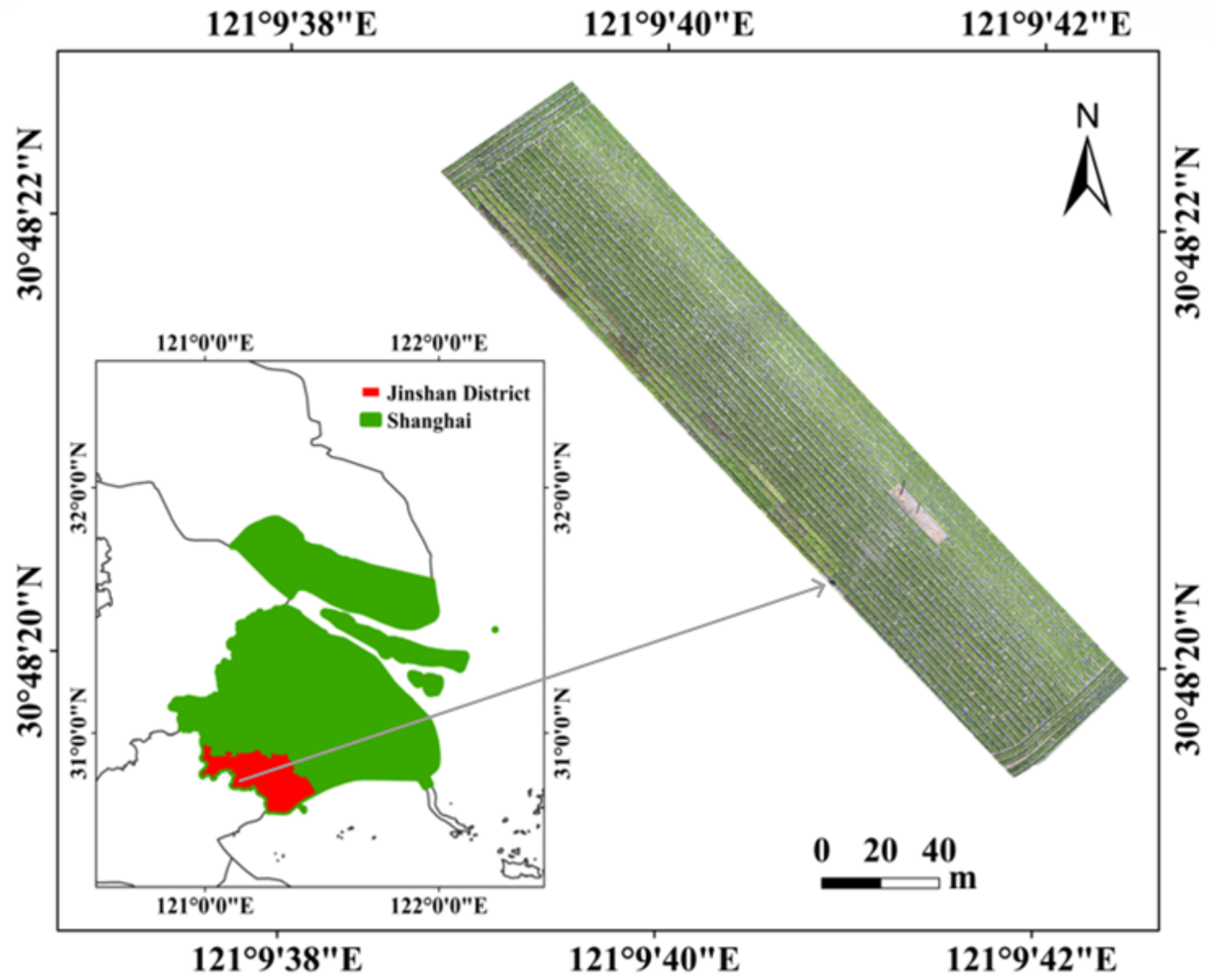
2.1. UAV-Based Lettuce RGB Images Acquisition

The experimental data were collected from a lettuce field in Jinshan District (30.805° N, 121.160° E), Shanghai, China. This study area is situated in the alluvial plain of the Yangtze River Delta and experiences a northern subtropical monsoon climate. Figure 1 shows the location of the selected lettuce field, where a single variety of lettuce from this field was chosen as the study object. In this field, all lettuce was sown on 9 February 2021 and harvested on 21 April 2021. The experiment was conducted during the lettuce harvesting period using a small consumer drone (DJI Mavic 2 professional drone, shot at a height of 15 m above the ground) and a total of 487 raw images with a resolution of 5472 × 3648 were captured according to a pre-planned flight plan and saved in a JPG format.

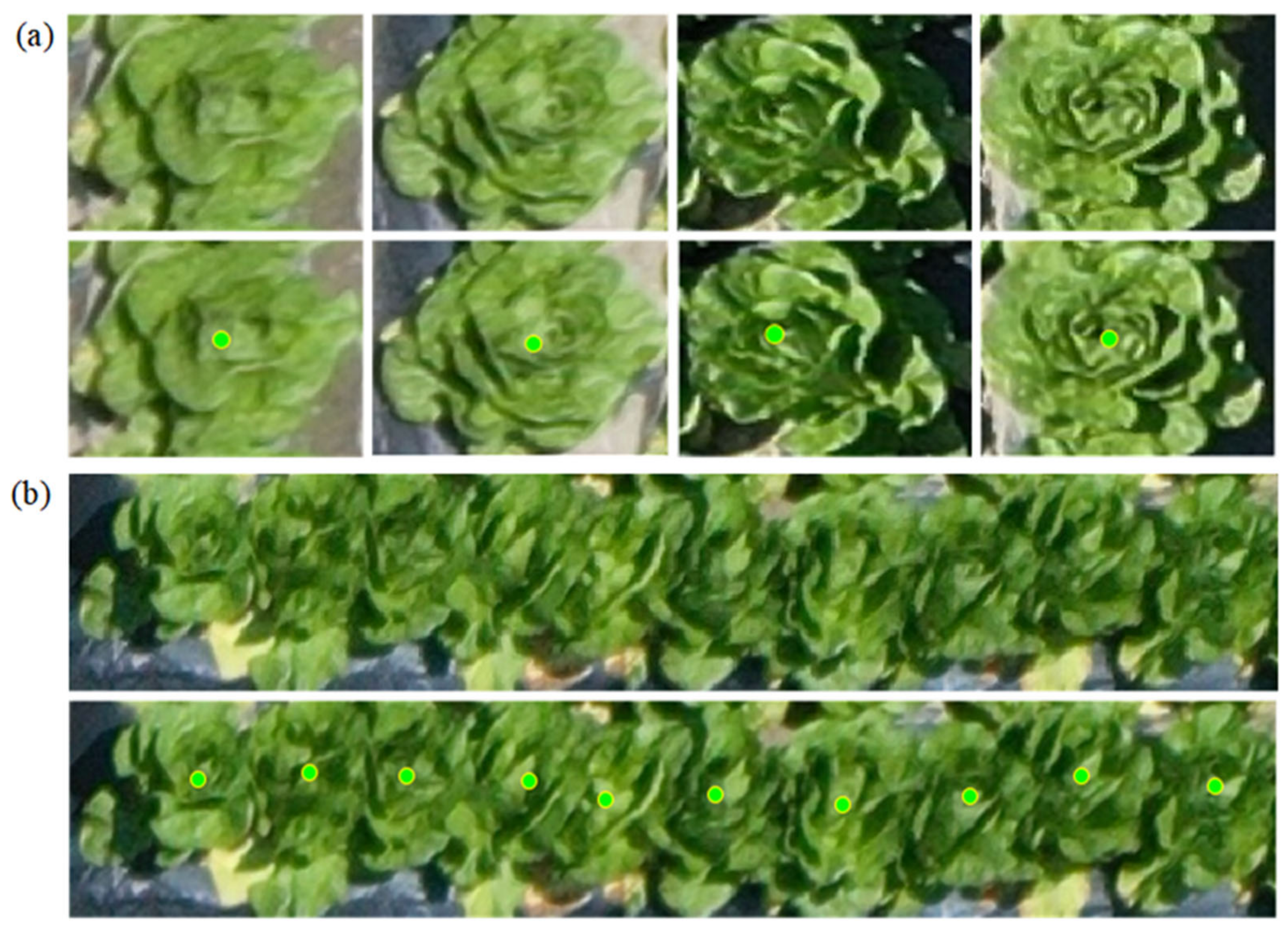
2.2. Lettuce Dataset Construction and Preprocessing

For the construction of the proposed LettuceNet, this study built a large-scale UAV-based lettuce dataset, the Shanghai Academy of Agricultural Sciences—Lettuce (SAAS-L), which contains 120 RGB images (resolution 5472 × 3648, with an average of 1348 lettuces per image) and 161,760 point-level annotations. The SAAS-L dataset encompasses a diverse range of lighting conditions, including lettuces exposed to direct sunlight, oblique sunlight, and cloudy skies. Additionally, these groups also exhibit significant variation in sparsity, with some lettuce populations having indistinguishable boundaries, while others can be clearly differentiated. During image capture, a relatively short shooting interval was set to ensure that each image has a high overlap rate. For UAV image capture, the front overlap rate was set to 80%, and the side overlap rate was set to 70%. This high overlap rate facilitates the stitching of captured images into a complete aerial image of the lettuce field through computer processing. However, for model training, images with a high overlap rate contain a significant number of redundant features, which can waste computational resources. To address this, 120 images with relatively low overlap rates were selected from the highly overlapping data collected. These 120 images were used for model training and testing, ensuring comprehensive coverage of the entire lettuce field. According to the experimental requirements, we used the labelme labels tool (http://labelme.csail.mit.edu/Release3.0/, accessed on 15 December 2022) to interactively label the high-resolution images of the dataset. In the labeling process, closely spaced lettuce plants are distinguished by their structural features. A single point is marked for point-level labels on each healthy lettuce variety, as illustrated in Figure 2. These points are labeled as “lettuce,” and a JSON file is generated for the original image, containing the coordinates of each marked point. The point-level labeling approach is more time-efficient than multi-point labels or bounding-box labeling.

To facilitate the model training, we adopted the method of Petti and Li. [10], by cropping 120 full high-resolution images (5472 × 3648) into 1920 non-overlapping images with a resolution of 1368 × 912 for the training, validation, and testing of the model, enhancing the counting accuracy. Finally, the SAAS-L dataset was divided into training, validation, and test sets in a 7:1:2 ratio, which consists of 84 training, 12 validation, and 24 test images with 1344, 192 and 384 sub-images, respectively. To boost model stability and prevent overfitting, we applied random image flipping and rotation as data augmentation techniques on the training set.

2.3. LettuceNet Structure

This study presents a model called LettuceNet, which is specifically designed to perform counting tasks on highly adherent lettuce plants. The proposed LettuceNet network architecture consists of four main components: the feature extraction module (FEM), the multi-scale feature fusion module (MFFM), the decoder module (DM), and the localization and counting module (LCM) (Figure 3). To improve the overall operational efficiency of the model, an improved MobileNetV2 is proposed in this study and introduced as a backbone network in the FEM module of LettuceNet. This MobileNetV2 was originally proposed by Sandler et al. [11], as a lightweight backbone network.

The LettuceNet architecture performs localization and counting tasks through the following process: RGB lettuce images are input into the Feature Extraction Module (FEM) to obtain multi-scale semantic feature maps. The deepest feature map from the FEM is then fed into the Multi-scale Feature Fusion Module (MFFM), which employs an Atrous Spatial Pyramid Pooling (ASPP) structure [12] to generate a multi-scale fusion feature map. The Decoder Module (DM) then fuses and up samples the multi-scale feature maps from the MFFM and the three shallow-scale feature maps from the FEM, producing feature maps rich in semantic information. Finally, after training, the Localization and Counting Module (LCM) predicts the location and quantity of lettuce based on the semantically rich feature maps. The following sections give detailed descriptions of the four main modules that constitute the LettuceNet model.

2.3.1. FEM

MobileNetV2 is a lightweight convolutional neural network that builds on v1 by introducing Linear Bottleneck and Inverted Residual to improve the network’s representation [13]. In this research, we improved MobileNetV2 as the main body of the FEM module of the LettuceNet, and the main improvements are as follows: (1) keep only the first eight convolutional layers in MobileNetV2 and add bias terms to each of them; (2) replace all Batch Normalization (BN) layers in MobileNetV2 with Group Normalization (GN) layers. LettuceNet is mainly designed to improve the accuracy of lettuce counting, while the deeper and higher dimensional features would increase the computation. Adding bias to the convolutional layer is essential to increase the expressiveness of the model, improve learning flexibility, break the symmetry of weight updates, and optimize the model to capture non-linear relationships. However, adding bias and using BN layers often cannot be done at the same time. This is because the presence of BN layers eliminates the role of bias and wastes computational resources in a way that GN layers do not. Moreover, the effect of BN layers on the model accuracy is very much dependent on batch_size; when batch_size is small, the accuracy of the model using BN layers is extremely degraded, and the model using BN layers does not support the case where batch_size is one [14]. Therefore, in our proposed LettuceNet, we use the GN layer instead of the BN layer to avoid over-dependence of model accuracy on batch_size.

The improved MobileNetV2 structure is as follows: as in Figure 4, the improved MobileNetV2 uses the inverted residual structure for the 2nd to 8th convolutional layers. Where expansion_factor is the expansion multiplier of the number of channels in the inverted residual structure and bottleneck_num is the number of cycles of the inverted residual structure. Improved MobileNetV2 performs a dimension boosting operation in the head convolution (a 1 × 1 conv, a GN layer and an activation function ReLU6) of the inverted residual structure to extract the features in the high-dimensional space. Then, a depth wise convolution is performed in the body convolution (a 3 × 3 DW conv, a GN layer and an activation function ReLU6) of the inverted residual structure in order to reduce the number of references and the computational cost, while improving the speed and performance of the operation. Finally, dimensionality reduction is performed in the tail convolution (a 1 × 1 DW conv and a GN layer) of the inverted residual structure. The first convolutional layer of Improved MobileNetV2 consists of a 3 × 3 DW Conv, a GN layer and a ReLU6 activation function. In addition, the improved MobileNetV2 adds bias to all convolutional layers and uses ReLU6 activation functions for the last seven convolutional layers to improve robustness. Among them, layer3, layer4, layer5 and layer8 of Improved MobileNetV2 are used as feature output layers to output feature maps in MFFM and DM modules, and their down sampling multiples are 1/4, 1/8, 1/16 and 1/32, respectively.

2.3.2. MFFM

The MFFM receives L4 from the FEM output (Figure 3), which consists of an ASPP structure containing a 1 × 1 Conv, three Atrous convolutional layers [15] with expansions of 6, 12, and 18, and a pooling layer. Among them, three Atrous convolutions provide a larger receptive field to capture multi-scale features. To fuse the multi-scale feature information output by ASPP, the feature fusion method concat is used, and then 1 × 1 Conv is used for channel compression, which finally outputs a 256-channel feature map to the DM.

2.3.3. DM

The input to the DM consists of the feature maps output from layers 3–5 in the FEM and the feature maps output from the MFFM (Figure 3). The decoding process of DM is similar to that of U-Net [16] and SegNet [17], where we perform double up sampling using bilinear interpolation, with a double up sampling operation immediately followed by a concat operation, instead of using direct summation for dimensional fusion. Next, the fusion features are convolved and downscaled using the cat_conv operation. The convolution operation helps the network learn the spatial structure of the input data, which enables the model to better understand and represent complex image information. After three rounds of progressive up sampling, concat and cat_conv, we downsize the feature maps using 1 × 1 Conv once and perform a quadruple up sampling of the down sampled feature maps to restore them to the original dimensions, and finally we obtain high quality feature maps (also a matrix) which are output to the LCM.

2.3.4. LCM

The LCM generates a binary mask F based on the input probability matrix Z, which represents whether each pixel belongs to the lettuce class (L). The definition formula for pixel F_ik is as follows (Equation (1)):

$${\mathrm{F}}_{\mathrm{i}\mathrm{k}}=\left\{\begin{array}{c}1, \mathrm{if} {\mathrm{Z}}_{\mathrm{i}\mathrm{k}}\ge 0.5\\ 0, \mathrm{if} {\mathrm{Z}}_{\mathrm{i}\mathrm{k}}< 0.5\end{array}\right.$$

(1)

where the F_ik represents the value of the pixel in column k of row i in the binary mask F; Z_ik is the probability that the pixel in row i, column k of the input probability matrix Z belongs to the lettuce class. After conducting several experiments, the model demonstrates optimal performance with a threshold set at 0.5.

In other words, if a pixel’s probability of belonging to the L is greater than or equal to 0.5, it is marked as 1 in the binary mask; otherwise, it is marked as 0. In this way, the LCM generates the corresponding binary mask F based on the probability matrix Z. Subsequently, adjacent pixels labeled as 1 are grouped according to the binary mask F and the connected component algorithm [18], forming contiguous regions known as blobs. These blobs correspond to individual heads of lettuce, with their number reflecting the quantity of lettuce and their positions indicating the spatial locations of the lettuce plants.

2.3.5. Loss Functions

The proposed LettuceNet is used for lettuce localizing and counting tasks by predicting and generating individual blobs. Loss functions commonly used for counting including focus loss, cross-entropy (CE) loss, and multitasking loss [19,20,21] are not applicable to the LettuceNet model because they do not enable the model to obtain useful information from point-labelled images. Therefore, this study uses a localization-based count loss function (LC-Loss) [22]. The LC-Loss is a hybrid loss function that requires only point-level labels representing the target location without size and shape. In the case of point-only labels, it outputs a blob for each target instance. The specific formula for LC-Loss is as follows (Equation (2)):

$$\mathrm{L}\left(\mathrm{S},\mathrm{T}\right)={\mathrm{L}}_{\mathrm{I}}\left(\mathrm{S},\mathrm{T}\right)+{\mathrm{L}}_{\mathrm{P}}\left(\mathrm{S},\mathrm{T}\right)+{\mathrm{L}}_{\mathrm{S}}\left(\mathrm{S},\mathrm{T}\right)+{\mathrm{L}}_{\mathrm{F}}\left(\mathrm{S},\mathrm{T}\right),$$

(2)

where, T represents the true matrix, labeled with points at the location of each target; S represents the output matrix, where each element represents the probability that the pixel point belongs to the lettuce class; and the L_I (Image-Level Loss) and L_P (Point-Level Loss) are loss functions for weakly supervised semantic segmentation algorithms [23].

The specific formulas for L_I and L_P are as follows (Equations (3) and (4)):

$${\mathrm{L}}_{\mathrm{I}}\left(\mathrm{S},\mathrm{T}\right)=-{\displaystyle \frac{1}{\left|{\mathrm{C}}_{\mathrm{e}}\right|}}{\sum }_{\mathrm{c}\in {\mathrm{C}}_{\mathrm{e}}}\mathrm{l}\mathrm{o}\mathrm{g}({\mathrm{S}}_{{\mathrm{t}}_{{\mathrm{c}}^{\mathrm{c}}}})-{\displaystyle \frac{1}{\left|{\mathrm{C}}_{\neg \mathrm{e}}\right|}}{\sum }_{\mathrm{c}\in {\mathrm{C}}_{\neg \mathrm{e}}}\mathrm{l}\mathrm{o}\mathrm{g}(1-{\mathrm{S}}_{{\mathrm{t}}_{{\mathrm{c}}^{\mathrm{c}}}}),$$

(3)

$${\mathrm{L}}_{\mathrm{p}}\left(\mathrm{S},\mathrm{T}\right)=-{\sum }_{\mathrm{i}\in {\mathrm{I}}_{\mathrm{s}}}\mathrm{l}\mathrm{o}\mathrm{g}\left({\mathrm{S}}_{\mathrm{i}{\mathrm{T}}_{\mathrm{i}}}\right),$$

(4)

where, C_e is the set of classes present in the image and C_¬e is the set of classes that are not present in the image. The L_I increases the probability that the model will predict a pixel to be in the Lettuce class. The L_P encourages the model to correctly label the supervised pixel points in the matrix T.

The last two items, L_S (Split-Level Loss) and L_F (False Positive Loss) allow the model to output a separate blob for each target instance and to remove blobs without target instances. The L_S uses the watershed segmentation algorithm [24] to suppress blobs whose model output contains more than or equal to two labeled points. The specific formulas for L_S and L_F are as follows (Equations (5) and (6)):

$${\mathrm{L}}_{\mathrm{S}}(\mathrm{S},\mathrm{T})=-{\sum }_{\mathrm{i}\in {\mathrm{T}}_{\mathrm{b}}}{\mathrm{a}}_{\mathrm{i}}\mathrm{l}\mathrm{o}\mathrm{g}\left({\mathrm{S}}_{\mathrm{i}0}\right),$$

(5)

$${\mathrm{L}}_{\mathrm{F}}(\mathrm{S},\mathrm{T})=-{\sum }_{\mathrm{i}\in {\mathrm{B}}_{\mathrm{f}\mathrm{p}}}\mathrm{l}\mathrm{o}\mathrm{g}\left({\mathrm{S}}_{\mathrm{i}0}\right),$$

(6)

where T_b is the set of segmentation boundaries; S_i0 is the probability that pixel i belongs to the background, and α_i is the number of labeled points in the blob to which pixel i belongs; L_F prevents the model from predicting blobs that do not contain labeled points to reduce the number of false positive predictions; and B_fp is the set of pixel points that make up the blobs, but these blobs do not contain labeled points.

2.4. Implementation Details and Accuracy Rating

This research is implemented using the PyTorch (1.13.1) framework and an NVIDIA Quadro P5000 (16 GB) GPU (NVIDIA, located in Santa Clara, CA, USA). The initial learning rate and batch size are set to 0.0001 and 1, respectively. During training, model parameters are adjusted based on the validation set performance using the ReduceLRonPlateau learning rate adjustment strategy, with the validation loss monitored in “min” mode, Patience set to 5, and Factor set to 0.9. If the validation loss does not decrease for five consecutive rounds, the learning rate is scaled to 0.9 of its original value. The Adam optimizer, a computationally efficient stochastic optimization method with low memory requirements, is used. To avoid overfitting, the dropout ratio is set to 0.2. After several rounds of experimental validation, the model reaches optimal convergence after 30 training epochs.

In this study, the coefficient of determination (R²), mean absolute error (MAE), root mean square error (RMSE) and normalized root mean square error (nRMSE) are used as evaluation metrics for LettuceNet counting. These metrics are calculated as follows (Equations (7)–(10)):

$$\mathrm{M}\mathrm{A}\mathrm{E}={\displaystyle \frac{1}{\mathrm{n}}}{\sum }_{\mathrm{i}=1}^{\mathrm{n}}{|\mathrm{t}}_{\mathrm{i}}-{\mathrm{p}}_{\mathrm{i}}|,$$

(7)

$$\mathrm{R}\mathrm{M}\mathrm{S}\mathrm{E}=\sqrt{{\displaystyle \frac{1}{\mathrm{n}}}{\sum }_{\mathrm{i}=1}^{\mathrm{n}}{{(\mathrm{t}}_{\mathrm{i}}-{\mathrm{p}}_{\mathrm{i}})}^2},$$

(8)

$$\mathrm{n}\mathrm{R}\mathrm{M}\mathrm{S}\mathrm{E}={\displaystyle \frac{\mathrm{R}\mathrm{M}\mathrm{S}\mathrm{E}}{\mathrm{m}\mathrm{a}\mathrm{x}\left(\mathrm{t}\right)-\mathrm{m}\mathrm{i}\mathrm{n}\left(\mathrm{t}\right)}},$$

(9)

$${\mathrm{R}}^2=1-{\displaystyle \frac{\sum _{\mathrm{i}=1}^{\mathrm{n}}{({\mathrm{t}}_{\mathrm{i}}-{\mathrm{p}}_{\mathrm{i}})}^2}{{\sum _{\mathrm{i}=1}^{\mathrm{n}}({\mathrm{t}}_{\mathrm{i}}-\overline{\mathrm{p}})}^2}},$$

(10)

where n is the total number of samples in the test set; t is the manual counting of true values; and $\overline{\mathrm{p}}$ is the model’s prediction of the number of lettuces in the test sample.

In addition, since robust localization is useful for agricultural applications in computer vision, the F-Score metric is used to evaluate the localization performance of LettuceNet. F-Score is a standard measure for detection as it considers both precision and recall, calculated using the following formula (Equation (11)):

$$\mathrm{F}-Score={\displaystyle \frac{2\mathrm{T}\mathrm{P}}{2\mathrm{T}\mathrm{P}+\mathrm{F}\mathrm{P}+\mathrm{F}\mathrm{N}}}$$

(11)

where the number of true positives (TP) is the number of blobs that contain at least one point label; the number of false positives (FP) is the number of blobs that contain no point label; and the number of false negatives (FN) is the number of point labels minus the number of true positives.

3. Results

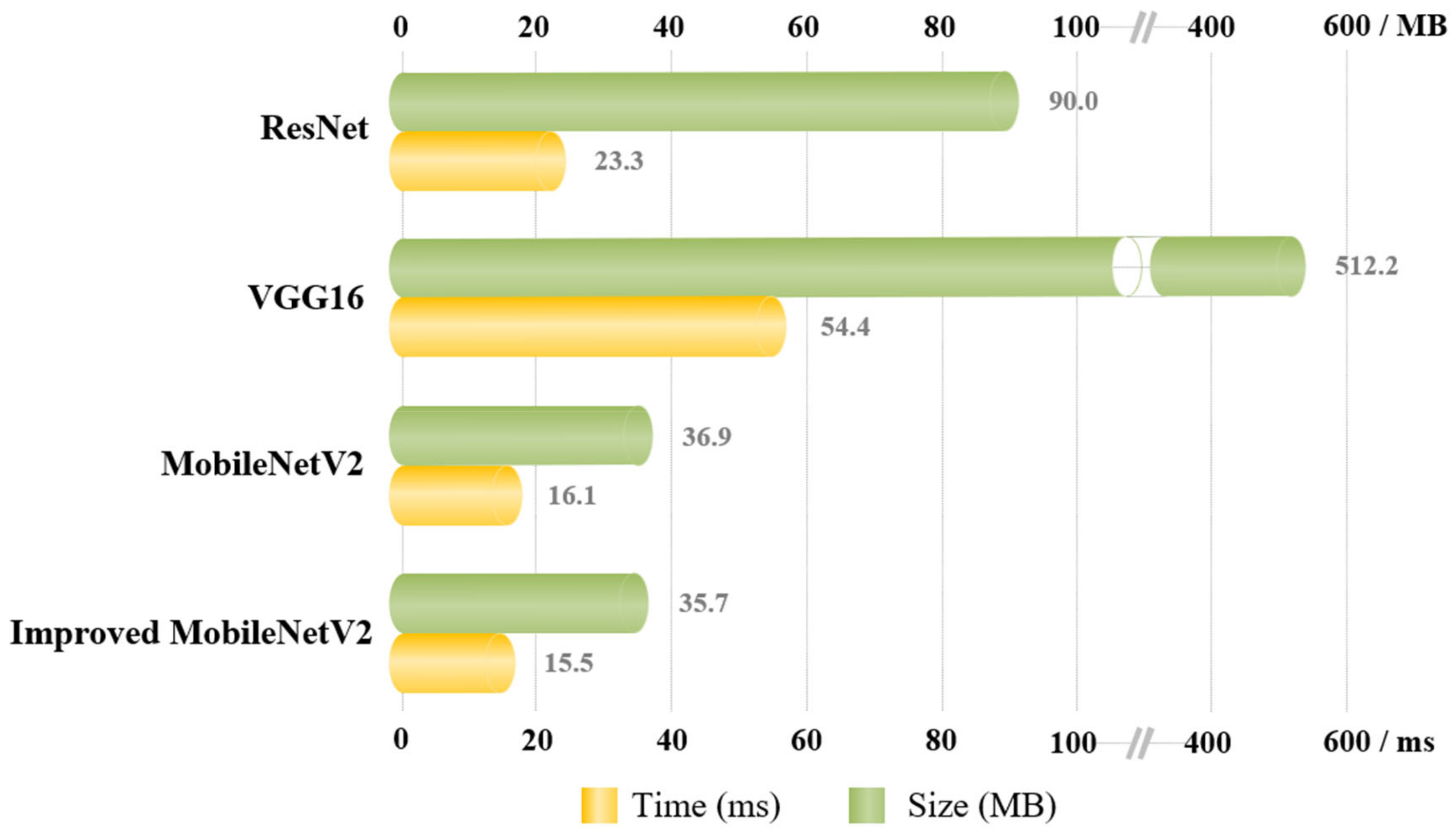
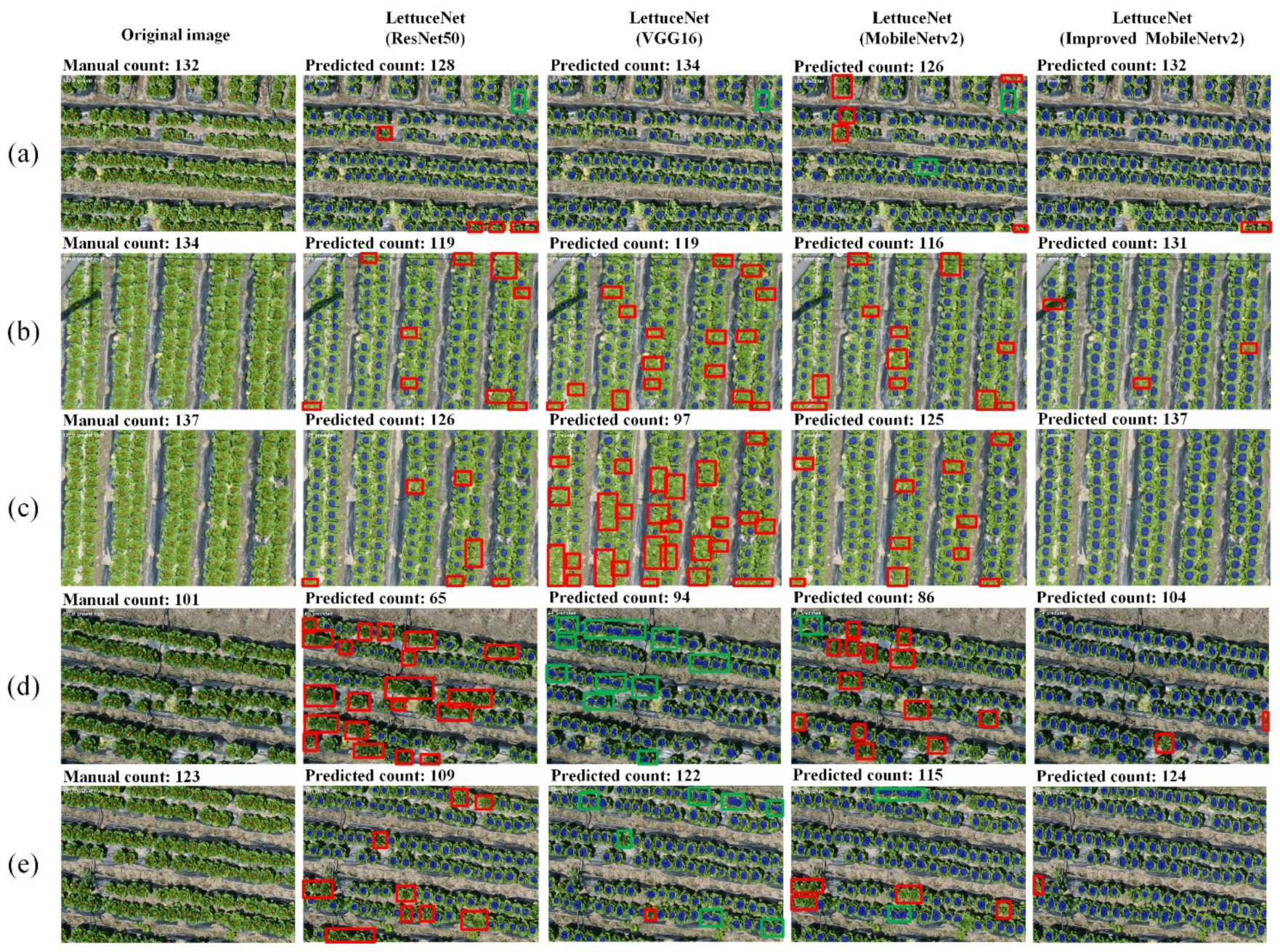
3.1. Evaluation of the Accuracy and Efficiency of LettuceNet Counting

To verify whether our improved MobileNetV2 can enable LettuceNet to achieve better performance, the counting accuracies of LettuceNet using different backbone networks are compared on the SAAS-L dataset (

Table 1. Count performance of different backbone networks on the SAAS-L dataset.

Backbone	Venue, Year	MAE	RMSE	nRMSE	R2
ResNet50	CVPR, 2009	8.5391	12.7231	0.0877	0.9328
VGG16	ICLR, 2015	10.9140	18.8136	0.1297	0.8531
MobileNetV2	CVPR, 2018	7.7042	11.2965	0.0780	0.9469
Improved MobileNetV2	This study	2.4486	4.0247	0.0276	0.9933

), including the classical Residual Network with 50 layers (ResNet50) [25], Visual Geometry Group 16 (VGG16) [26], and MobileNet Version 2 (MobileNetV2) [11]. The results indicate that LettuceNet equipped with the improved MobileNetV2 as the backbone network achieves the better performance, with the counting accuracy of MAE, RMSE, nRMSE and R² being 2.4486, 4.0247, 0.0276 and 0.9933, respectively.

In addition, the results of model operation efficiency comparison show that LettuceNet performs better when equipped with improved MobileNetV2 as the backbone network. As shown in Figure 5, it is found that the size of the LettuceNet model using the improved MobileNetV2 as the backbone is about 35.7 MB, which is 60.33%, 93.03% and 3.25% lower than the size of the LettuceNet model using ResNet50, VGG16 and MobileNetV2 as the backbone, respectively. In addition, the efficiency of the model is evaluated by calculating the time taken to test multiple images and using the average time. The average processing time is approximately 15.5 ms, which is 33.40%, 71.49%, and 3.72% less than the time of the LettuceNet model using ResNet50, VGG16, and MobileNetV2 as the backbone, respectively.

To evaluate the validity of the model improvement in this study, the corresponding ablation experiments were performed. As shown in

Table 2. Comparison of counting performance under different normalization methods.

Backbone	Normalization Method	MAE	RMSE	nRMSE	R2
ResNet50	BN	8.5391	12.7231	0.0877	0.9328
VGG16	BN	10.9140	18.8136	0.1297	0.8531
MobileNetV2	BN	7.7042	11.2956	0.0780	0.9469
ResNet50	GN	2.7196	4.0846	0.0282	0.9930
VGG16	GN	3.9307	6.1983	0.0427	0.9841
Improved MobileNetV2	GN	2.4486	4.0247	0.0276	0.9933

, normalizing with GN significantly improves LettuceNet’s performance. When using Res-Net50 as the backbone, the MAE is reduced to 2.7196, RMSE to 4.0846, nRMSE to 0.0282, and R² is improved to 0.9930. With VGG16 as the backbone, the MAE is reduced to 3.9307, RMSE to 6.1983, nRMSE to 0.0427, and R² is improved to 0.9841. The proposed LettuceNet achieves better evaluation metrics when equipped with the improved MobileNetV2 under different normalization methods.

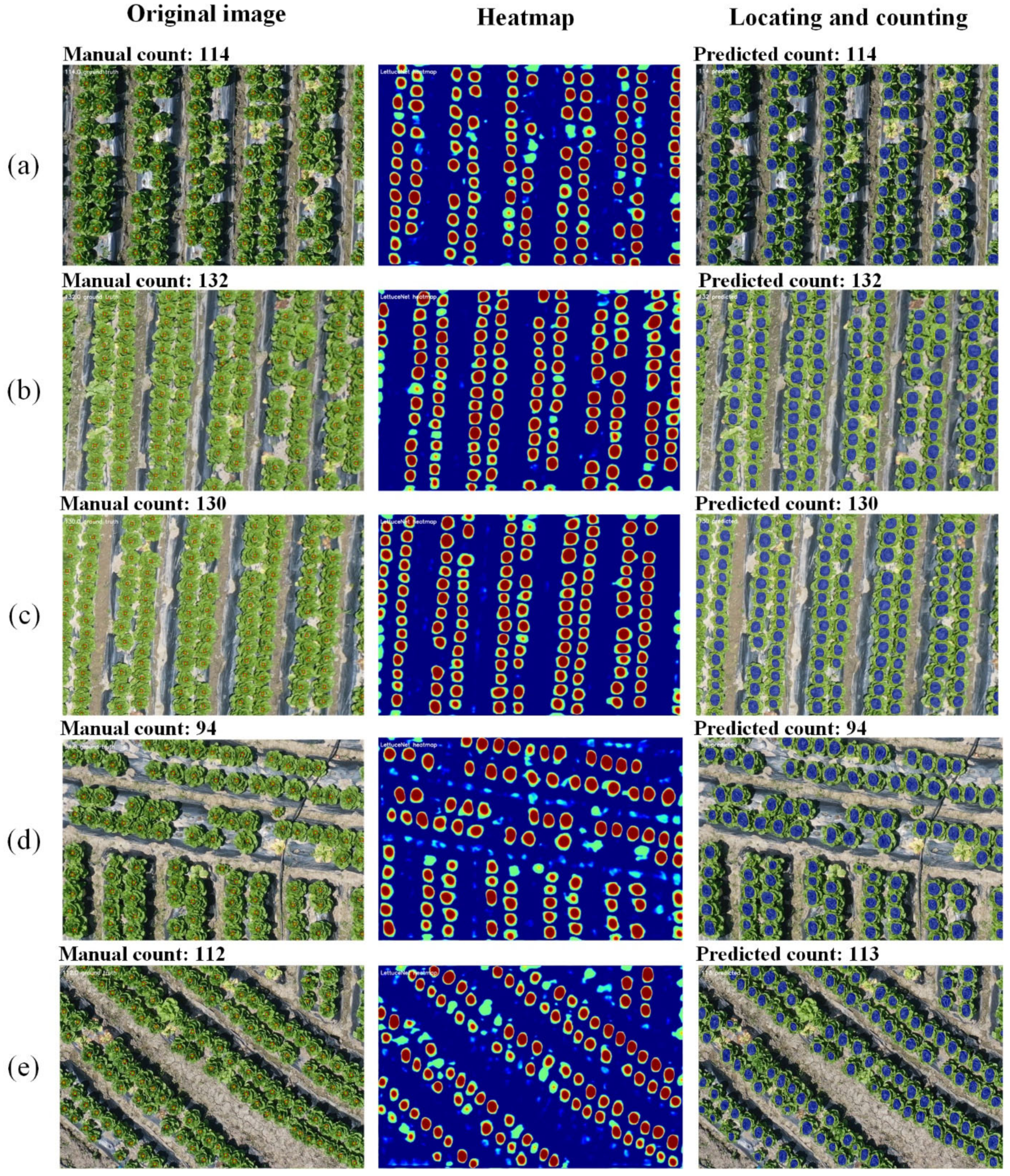
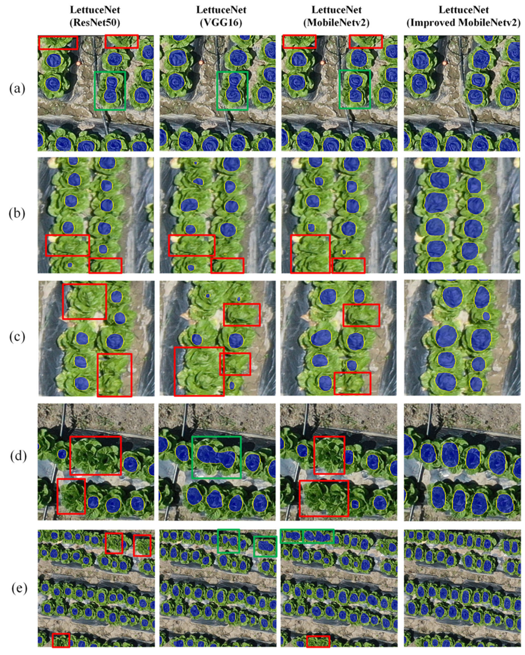
3.2. Localization Evaluation of LettuceNet

Figure 6 shows the localization effect of the LettuceNet model using the improved MobileNetV2 as the backbone for lettuce counts on the SAAS-L dataset. It can be seen that LettuceNet can complete the task of lettuce localization and counting under different sparsity levels and different light intensities. Meanwhile, the area and degree of interest of the LettuceNet model could be visualized clearly from the heat map.

Figure 7 and Figure 8 further examine the effectiveness of LettuceNet’s localization in lettuce images with different border and texture features, as well as varying degrees of tight arrangement. As shown in

Table 3. Localization performance of different backbone networks on the SAAS-L dataset.

Backbone	F-Score	Increase Rate over Improved MobileNetV2
ResNet50	0.8943	−8.68%
VGG16	0.8227	−15.93%
MobileNetV2	0.9156	−6.44%
Improved MobileNetV2	0.9791	\

, the F-Score of the LettuceNet model with the improved MobileNetV2 as the backbone is 0.9791, while that of the LettuceNet models with ResNet50, VGG16 and MobileNetV2 as the backbone is 0.8943, 0.8227, and 0.9156, respectively. The results indicate that the LettuceNet using the improved MobileNetV2 as the backbone network could complete the lettuce localization tasks in scenes with different boundary and texture features and different tightness of lettuce arrangements.

According to Figure 7 and Figure 8, LettuceNet with ResNet50, VGG16, and MobileNetV2 as the backbone networks encounters issues in locating lettuce images with tight arrangements. Specifically, LettuceNet with VGG16 as the backbone network exhibits a small number of false positives in the prediction results (row 1, Figure 8). In contrast, LettuceNet (rows 2–3, Figure 8) using ResNet, VGG16, and MobileNetV2 as the backbone network would have a large number of missed detections for lettuce images with unclear borders, and fuzzy texture features. In the localization of overly tightly arranged lettuce (rows 4–5, Figure 8), LettuceNet using ResNet50 and MobileNetV2 as the backbone networks (red boxes) suffers from varying degrees of missing detections, whereas LettuceNet using VGG16 as the backbone network appears to recognize multiple lettuces as a single one (green boxes).

3.3. Comparison of LettuceNet with Existing Similar Methods

The proposed LettuceNet is further compared in terms of accuracy with five representative point-supervised advanced network architectures that could be used for lettuce counting, including Multi-Column Convolutional Neural Network (MCNN) [27], Extended Convolutional Neural Networks (CSRNets) [28], Scale Aggregation Network (SANet) [29], TasselNet version 2 (TasselNetV2) [30] and Focused Inverse Distance Transformation Map (FIDTM) [31]. The performance comparison of lettuce counting using these methods on the SAAS-L dataset is given in

Table 4. Performance of different methods on the SAAS-L dataset.

Method	Venue, Year	MAE	RMSE	nRMSE	R2
MCNN	CVPR, 2016	21.6751	24.3227	0.1742	0.3569
CSRNet	CVPR, 2018	11.6435	14.8340	0.1065	0.8502
SANet	ECCV, 2018	10.2312	13.8073	0.1016	0.8769
TasselNetV2	PLME, 2019	19.5449	20.1694	0.1568	0.4132
FIDTM	Arxiv, 2021	17.8176	18.4937	0.1421	0.5765
LettuceNet	This study	2.4486	4.0247	0.0276	0.9933

, and the results indicate that the LettuceNet has the better performance in all evaluation metrics, with 13.27% higher R² and 72.83% lower nRMSE compared to the second most accurate SANet in terms of counting accuracy.

Moreover, the LettuceNet is further compared with these above five counting methods in terms of the model operation efficiency (Figure 9), and the results indicate that the LettuceNet has slightly lower operation efficiency than the MCNN, SANet, and TasselNetV2 in terms of running time and model size, but its operation efficiency is much higher than CSRNets and FIDTM. As shown in Figure 9, the LettuceNet tests a single image at 15.5 ms, which is slightly slower than MCNN, SANet, and TasselNetV2 with 1.1 ms, 6.8 ms, and 2.1 ms, respectively, but much faster than CSRNets and FIDTM with 119.5 ms, and 529.6 ms. Overall, the comparison with other existing similar counting method results indicates that the proposed LettuceNet has the higher accuracy and relatively high model operation efficiency.

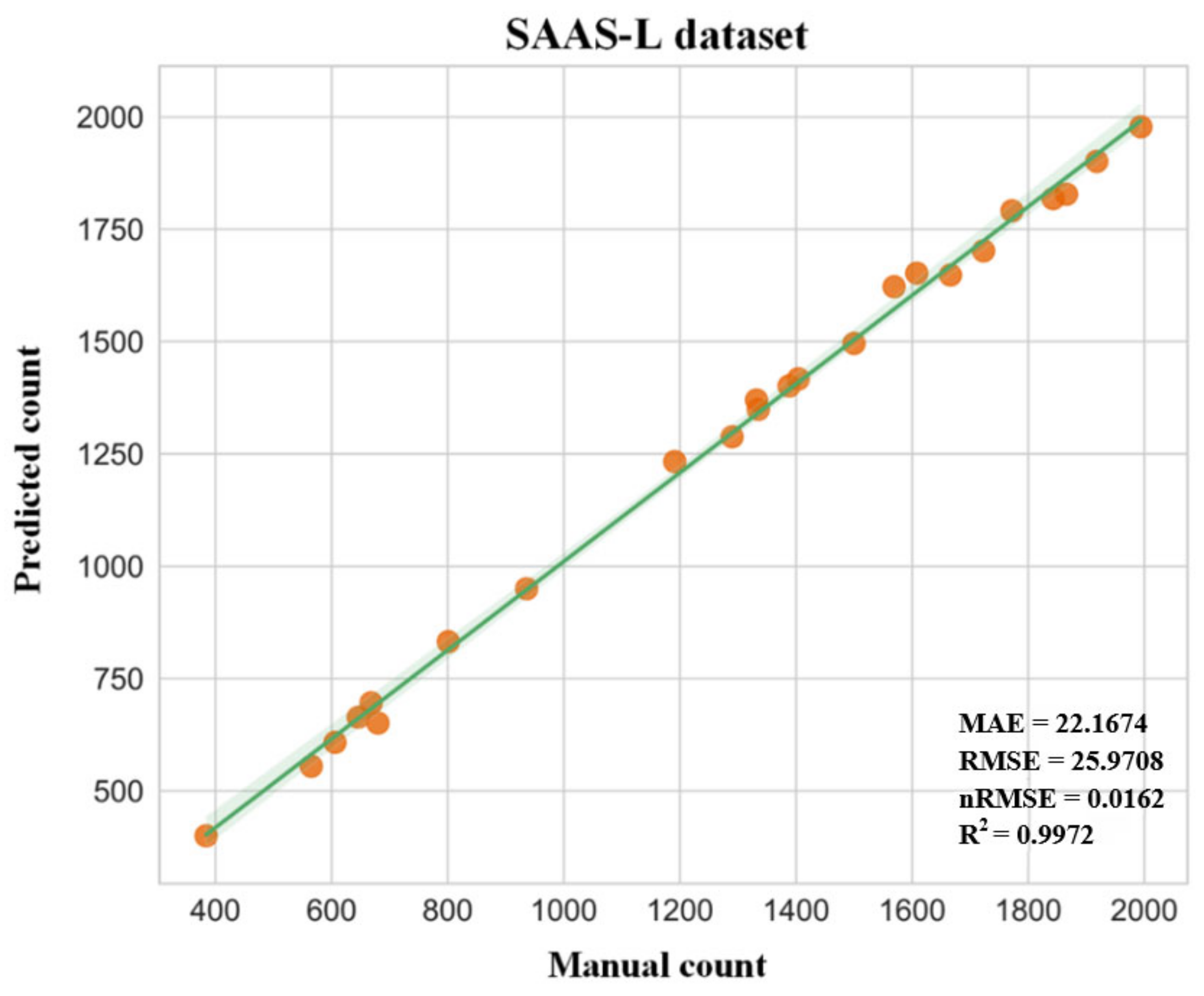
3.4. Generalizability Evaluation of LettuceNet

The ability to show good performance under different datasets is related to whether LettuceNet can be extended to other application scenarios. To further validate the generalization capability of LettuceNet and its counting accuracy in non-specific environments, additional experiments were conducted on the Global Wheat Head Detection (GWHD) dataset (https://www.global-wheat.com/index.html, accessed on 21 February 2024). In this validation experiment, the LettuceNet was used alone for training and testing on the GWHD dataset. A total of 2041 images were randomly selected from the GWHD dataset as the training set, and 451 images were used as the test set. The original resolution of those images is 1024 × 1024. The number of wheat heads in each image varies from 3 to around 120.

Table 5. Performance of different methods on the GWHD dataset.

Method	Venue, Year	MAE	RMSE	nRMSE	R2
MCNN	CVPR, 2016	13.4583	14.7319	0.2096	0.7262
CSRNet	CVPR, 2018	6.9403	8.4934	0.1347	0.8868
SANet	ECCV, 2018	12.0519	14.0147	0.1972	0.7419
TasselNetV2	PLME, 2019	5.1772	6.1824	0.0982	0.9357
FIDTM	Arxiv, 2021	10.1745	11.6043	0.1872	0.7876
LettuceNet	This study	5.8173	7.6048	0.1070	0.9057

gives the performance comparison between LettuceNet and other different counting methods on the test dataset of GWHD. The results indicate that the MAE, RMSE, nRMSE, and R² of LettuceNet are 5.8173, 7.6048, 0.1070, and 0.9057, respectively, which are very close to the performance of TasselNetV2, which is specifically used for wheat spikelet counting, and far outperforms the performance of MCNN, CSRNets, SANet and FIDTM.

Figure 10 displays the visual effects of LettuceNet’s counting of wheat heads on the GWHD dataset, showing that LettuceNet can also perform well in locating scenes with sparse objects. As shown in rows 1–3, Figure 10, the LettuceNet could identify and localize the wheat heads with obvious features and large differences from the background and has good object feature extraction and fusion between different feature levels. Although there are some false positives in LettuceNet’s prediction, as shown in rows 4–5, Figure 10, mainly because the wheat heads and the background with similar characteristics are mixed under strong light irradiation, and thus the LettuceNet predict plant leaves or weeds with similar characteristics to wheat heads as wheat heads. Overall, the performance of LettuceNet in wheat counting tasks is excellent and stable, which proves that LettuceNet exhibits strong generalization ability in non-specific environments.

3.5. Boundary Effects Evaluation of LettuceNet

Boundary effects are a significant factor impacting counting accuracy in target detection and image segmentation research. Similarly, the method in this study is inevitably influenced by boundary effects. In this study, LettuceNet was tested on 24 original lettuce images with a resolution of 5472 × 3648, randomly selected from the SAAS-L dataset. The manual counts for these images ranged from 400 to 2000 per image. To reduce hardware requirements for model training, each original lettuce image was segmented into 16 non-overlapping images with a resolution of 1368 × 912 during preprocessing, resulting in a total of 384 segmented sub-images. The counting results of these segmented sub-images were then stitched together to reconstitute the 24 original images.

The validation results, as shown in Figure 11, show that the counting accuracy R² (0.9972) for the 24 stitched lettuce images is comparable to that of the 384 test sub-images R² (0.9933), indicating that the proposed LettuceNet model is less affected by the boundary effects. Even though, compared with the manual count number, there will still be a certain degree of localization error, especially at the boundaries of image stitching. As shown in Figure 12, there were lettuces in the suture boundaries of the images that were not successfully localized and counted (A–C), which means that the model predicted some false positives or repeated localization and counting of the same target (D). In general, the proposed LettuceNet is less affected by boundary effects, which may be partly attributed to the fact that LettuceNet only accepts supervision from a single pixel point when training lettuce classes. When a lettuce has more than one prediction block, LettuceNet tries to reduce the redundant blocks; and when a lettuce does not have any prediction block corresponding to it, LettuceNet tries to generate a separate block for that lettuce.

4. Discussion

4.1. Advantages of LettuceNet

High-density lettuce planting patterns are widely applied in agricultural production, yet automated plant counting faces challenges due to the complex lighting variations in lettuce images captured by UAVs and the difficulty of annotating densely populated lettuce images. This limits the availability of high-quality, multi-point data required for strongly supervised DL methods. This study proposes the LettuceNet architecture and demonstrates its efficacy in the task of lettuce counting. The evaluation results show that the improved MobileNetV2, as the backbone of LettuceNet, achieves computation accuracy in terms of MAE, RMSE, nRMSE, and R² of 2.4486, 4.0247, 0.0276, and 0.9933, respectively, with a localization accuracy F-Score of 0.9791, surpassing traditional backbones such as MobileNetV2, ResNet50, and VGG16. This can be attributed to the use of different normalization methods and the application of inverted residual structures in the improved MobileNetV2, enhancing gradient propagation, and reducing inference time and memory usage [14,32]. Moreover, LettuceNet is based on point supervision, a weakly supervised method, requiring only one point label per lettuce during model training. This annotation method is less error-prone compared to multi-point and bounding box labels, as it only requires ensuring the point label is within each lettuce, without needing precise center placement. Additionally, the time cost of point label is significantly lower than that of multi-point and bounding box labels [33,34].

Although many advanced lightweight backbone networks have been proposed in recent years, MobileNetV2 as a classical module is still widely applied [35,36]. In this study, the improved MobileNetV2 is chosen over the latest backbone networks mainly due to its balanced performance in terms of accuracy, efficiency, and model stability. Although advanced backbone networks may improve model performance, the overall architectural design and its applicability to specific research and datasets are more critical [37,38]. As shown in Table 1, when LettuceNet uses the improved MobileNetV2 with lightweight and fewer parameters as the backbone network, it even outperforms the more advanced ResNet50 as the backbone network. This may be due to the superior model architecture and the inverted residual structure being more suitable for the lettuce counting task in this study; furthermore, some studies have shown that advanced backbone networks with more parameters and more complex structures do not necessarily perform better than lightweight and fewer parameter backbone networks [39,40,41].

In addition, since some previous point-supervised counting studies rarely used object detection or instance segmentation models as comparison models, this study selected five representative point-supervised counting models as comparison methods (Table 4), and the evaluation results indicate that LettuceNet outperforms the state-of-the-art counting methods, such as MCNN, CSRNets, SANet, TasselNetV2, and FIDTM. This is related to several advantages of LettuceNet’s network structure, including the incorporation of the ASPP structure in the MFFM module, the robust DM decoder structure, and the adoption of LC-Loss [42,43]. Compared to the MCNN, CSRNets, and other methods that capture randomly distributed targets, LettuceNet has an advantage in high-throughput crop phenotyping counting with uniform distributions. Additionally, Xiong et al. [30], embedded local visual context into TasselNetV2, enhancing its performance in the task of wheat spike counting. However, unlike the spatial overlap of wheat spikes, the closely arranged lettuce overlap on the same plane in the SAAS-L dataset makes TasselNetV2 less applicable, while LettuceNet embeds the watershed algorithm and improves counting accuracy through the fusion of local and global information.

Furthermore, while object detection and instance segmentation methods, such as YOLOV10 and the Segment Anything Model (SAM), are potential solutions, these methods rely on strong supervision training and require precise annotations, a complex process that is prone to errors, and are not suitable for dense and high-density lettuce counting [44,45]. In contrast, LettuceNet only requires point labeling for training, which is simpler, less error-prone, and has lower time costs.

In summary, LettuceNet delivers outstanding performance in lettuce counting and localization tasks through its innovative point-supervised training approach, unique model architecture, including the inverted residual structure and different normalization methods, providing a new solution for similar visual tasks.

4.2. Future Improvements for LettuceNet

Although the study results have demonstrated that LettuceNet achieves high accuracy in the localization and counting of high-density lettuce, there are still some issues that merit further investigation and optimization. Firstly, this study was particularly focused on the diversity factors of the environment where the lettuce population resides, such as planting distance, light intensity, shading degree, and the clarity of the boundaries between adjacent crops. These environmental factors have a significant impact on the accurate counting and localization of lettuce. To this end, the research team has collected a diverse dataset, SAAS-L, containing 161,760 lettuce samples. Moreover, the primary objective of this study was to achieve accurate lettuce counting and localization under actual field conditions with different environments, providing a foundation for future applications such as field yield estimation. Therefore, the experimental setting was designed with a single flight condition and a single growth stage, which is a common approach in many similar advanced studies [46,47,48]. However, the altitude of UAV flights, the flight posture, and the characteristic changes of lettuce at different growth stages are critical factors that can influence the practical application of UAV-related field feature detection tasks. To address this, we plan to collect and analyze a more comprehensive dataset covering a wider area and a broader range of lettuce at different growth and fertility stages, captured by UAVs at various flight altitudes. This expanded dataset will enable further validation of the generalization and robustness of the LettuceNet method.

Secondly, due to the adoption of a weakly supervised learning strategy, LettuceNet is unable to accurately predict the size and boundary details of lettuce. To address this issue, we plan to explore the application of object detection or instance segmentation models to the SAAS-L dataset, with the aim of achieving accurate area and boundary prediction for lettuce, while maintaining the accuracy of counting and localization.

Finally, we will further optimize the localization and counting capabilities of LettuceNet by selecting and improving more advanced backbone networks and loss functions, with the expectation of achieving accurate lettuce area and boundary prediction on the basis of weak supervision and conducting a comprehensive comparison and evaluation with advanced object detection and instance segmentation models.

5. Conclusions

In this study, based on a weakly supervised DL approach, a novel network, specifically for locating and counting high-density lettuce in UAV images, called LettuceNet, was developed on a large high-throughput dense lettuce image dataset. The proposed LettuceNet architecture employed an improved MobileNetV2 as the foundational backbone network, making it more advantageous for lightweight application scenarios. This improved MobileNetV2 serves as a feature extraction network, while the ASPP structure is utilized for fusing the semantic information at multiple levels to obtain a feature map with rich semantic information and reliability. Furthermore, within the LettuceNet architecture, a hybrid loss function, LC-Loss, is employed to support the localization and counting of lettuce based on point-level labels and to effectively differentiate highly overlapping lettuce. A comparative evaluation of LettuceNet that utilized different backbone networks, including ResNet50, VGG16, MobileNetV2, and the proposed improved MobileNetV2 for lettuce counting was conducted. The results showed that the LettuceNet model, utilizing the enhanced MobileNetV2 as the backbone network, achieved superior performance in counting accuracy, localization accuracy, and computational efficiency. Specifically, the counting accuracy metrics included a Mean Absolute Error (MAE) of 2.4486, Root Mean Squared Error (RMSE) of 4.0247, normalized RMSE (nRMSE) of 0.0276, and an R² of 0.9933. Additionally, the F-Score for localization accuracy reached 0.9791. In addition, the localization effect of the LettuceNet model using the improved MobileNetV2 as the backbone for lettuce counting indicates that the proposed LettuceNet could complete the localization and counting tasks for lettuce under different sparsity levels and different light irradiation.

Moreover, the proposed LettuceNet is further compared in terms of accuracy and efficiency with other advanced network architectures that could be used for plant counting, including MCNN, CSRNets, SANet, TasselNetV2, and FIDTM. The results indicate that the proposed LettuceNet has the higher accuracy and relatively high model operation efficiency, with 13.27% higher R² and 72.83% lower nRMSE compared to the second most accurate SANet in terms of counting accuracy.

Furthermore, the LettuceNet also performed well in the wheat counting task, with MAE, RMSE, nRMSE, and R² of 5.8173, 7.6048, 0.1070, and 0.9057, respectively, which was very close to the performance of TasselNetV2, which is specifically used for wheat spike counting, and this proved that LettuceNet has strong generalization ability in non-specific environments. In conclusion, our LettuceNet provides a cost-effective and efficient method to achieve efficient and accurate localization and counting of high-density lettuce in the field based on UAV images.

Given that there are currently limited model methods available for accurate localization and counting of high-density lettuce plants under high-throughput conditions, our proposed LettuceNet is of great significance to field management practices. Future research will concentrate on developing weakly supervised methods to enhance the accuracy of counting both complete and incomplete lettuce plants, as well as estimating the coverage area of high-density lettuce plants. Furthermore, there are plans to gather and analyze more comprehensive datasets encompassing a broader range of areas and multiple growth stages of lettuce, utilizing UAV-captured images at varying altitudes and angles to validate the generalization and robustness of the LettuceNet model.

References

1. Zhou, J.; Li, P.; Wang, J. Effects of Light Intensity and Temperature on the Photosynthesis Characteristics and Yield of Lettuce. Horticulturae 2022, 8, 178. [Google Scholar] [CrossRef]
2. de Oliveira, E.Q.; Neto, F.B.; de Negreiros, M.Z.; Júnior, A.P.B.; de Freitas, K.K.C.; da Silveira, L.M.; de Lima, J.S. Produção e valor agroeconômico no consórcio entre cultivares de coentro e de alface. Hortic. Bras. 2005, 23, 285–289. [Google Scholar] [CrossRef]
3. Khoroshevsky, F.; Khoroshevsky, S.; Bar-Hillel, A. Parts-per-Object Count in Agricultural Images: Solving Phenotyping Problems via a Single Deep Neural Network. Remote Sens. 2021, 13, 2496. [Google Scholar] [CrossRef]
4. Wu, J.; Yang, G.; Yang, X.; Xu, B.; Han, L.; Zhu, Y. Automatic Counting of in situ Rice Seedlings from UAV Images Based on a Deep Fully Convolutional Neural Network. Remote Sens. 2019, 11, 691. [Google Scholar] [CrossRef]
5. Bai, X.; Liu, P.; Cao, Z.; Lu, H.; Xiong, H.; Yang, A.; Cai, Z.; Wang, J.; Yao, J. Rice Plant Counting, Locating, and Sizing Method Based on High-Throughput UAV RGB Images. Plant Phenom. 2023, 5, 20. [Google Scholar] [CrossRef]
6. Li, Y.; Bao, Z.; Qi, J. Seedling maize counting method in complex backgrounds based on YOLOV5 and Kalman filter tracking algorithm. Front. Plant Sci. 2022, 13, 1030962. [Google Scholar] [CrossRef] [PubMed]
7. Feng, A.; Zhou, J.; Vories, E.; Sudduth, K.A. Evaluation of cotton emergence using UAV-based imagery and deep learning. Comput. Electron. Agric. 2020, 177, 105711. [Google Scholar] [CrossRef]
8. Machefer, M.; Lemarchand, F.; Bonnefond, V.; Hitchins, A.; Sidiropoulos, P. Mask R-CNN Refitting Strategy for Plant Counting and Sizing in UAV Imagery. Remote Sens. 2020, 12, 3015. [Google Scholar] [CrossRef]
9. Bauer, A.; Bostrom, A.G.; Ball, J.; Applegate, C.; Cheng, T.; Laycock, S.; Rojas, S.M.; Kirwan, J.; Zhou, J. Combining computer vision and deep learning to enable ultra-scale aerial phenotyping and precision agriculture: A case study of lettuce production. Hortic. Res. 2019, 6, 70. [Google Scholar] [CrossRef]
10. Petti, D.; Li, C.Y. Weakly-supervised learning to automatically count cotton flowers from aerial imagery. Comput. Electron. Agric. 2022, 194, 106734. [Google Scholar] [CrossRef]
11. Sandler, M.; Howard, A.; Zhu, M.; Zhmoginov, A.; Chen, L. MobileNetV2:Inverted Residuals and Linear Bottlenecks. In Proceedings of the 31st IEEE Conference on Computer Vision and Pattern Recognition (CVPR), Salt Lake City, UT, USA, 18–22 June 2018; pp. 4510–4520. [Google Scholar] [CrossRef]
12. Yang, M.; Yu, K.; Zhang, C.; Li, Z.; Yang, K. DenseASPP for Semantic Segmentation in Street Scenes. In Proceedings of the 31st IEEE/CVF Conference on Computer Vision and Pattern Recognition (CVPR), Salt Lake City, UT, USA, 18–22 June 2018. [Google Scholar] [CrossRef]
13. Howard, A.G.; Zhu, M.; Chen, B.; Kalenichenko, D.; Wang, W.; Weyand, T.; Andreetto, M.; Adam, H. MobileNets: Efficient Convolutional Neural Networks for Mobile Vision Applications. arXiv 2017, arXiv:1704.04861. [Google Scholar]
14. Wu, Y.; He, K.; He, K. Group Normalization. arXiv 2018, arXiv:1803.08494. [Google Scholar]
15. Yu, F.; Koltun, V. Multi-Scale Context Aggregation by Dilated Convolutions. arXiv 2016, arXiv:1511.07122. [Google Scholar]
16. Ronneberger, O.; Fischer, P.; Brox, T. U-Net:Convolutional Networks for Biomedical Image Segmentation. arXiv 2015, arXiv:1505.04597. [Google Scholar] [CrossRef]
17. Badrinarayanan, V.; Kendall, A.; Cipolla, R. Segnet: A deep convolutional encoder-decoder architecture for image segmentation. arXiv 2015, arXiv:1511.00561. [Google Scholar] [CrossRef] [PubMed]
18. Wu, K.; Otoo, E.; Shoshani, A. Optimizing connected component labeling algorithms. In Image Processing, Medical Imaging; SPIE: Bellingham, WA, USA, 2005; Available online: https://ui.adsabs.harvard.edu/abs/2005SPIE.5747.1965W/abstract (accessed on 12 November 2022).
19. Li, Z.; Li, Y.; Yang, Y.; Guo, R.; Yang, J.; Yue, J.; Wang, Y. A high-precision detection method of hydroponic lettuce seedlings status based on improved Faster RCNN. Comput. Electron. Agric. 2021, 182, 106054. [Google Scholar] [CrossRef]
20. Ghosal, S.; Zheng, B.; Chapman, S.C.; Potgieter, A.B.; Jordan, D.R.; Wang, X.; Singh, A.K.; Singh, A.; Hirafuji, M.; Ninomiya, S.; et al. A Weakly Supervised Deep Learning Framework for Sorghum Head Detection and Counting. Plant Phenom. 2019, 2019, 1525874. [Google Scholar] [CrossRef] [PubMed]
21. Afonso, M.; Fonteijn, H.; Fiorentin, F.S.; Lensink, D.; Mooij, M.; Faber, N.; Polder, G.; Wehrens, R. Tomato Fruit Detection and Counting in Greenhouses Using Deep Learning. Front. Plant Sci. 2020, 11, 571299. [Google Scholar] [CrossRef] [PubMed]
22. Laradji, I.H.; Rostamzadeh, N.; Pinheiro, P.O.; Vazquez, D.; Schmidt, M. Where Are the Blobs: Counting by Localization with Point Supervision. Comput. Vis.—ECCV 2018, 2018, 560–576. [Google Scholar] [CrossRef]
23. Bearman, A.; Russakovsky, O.; Ferrari, V.; Fei-Fei, L. What’s the Point: Semantic Segmentation with Point Supervision. In Proceedings of the 14th European Conference on Computer Vision (ECCV), Amsterdam, The Netherlands, 11–14 October 2016. [Google Scholar] [CrossRef]
24. Beucher, S.; Meyer, F. The morphological approach to segmentation: The watershed transformation. In Mathematical Morphology in Image Processing; CRC Press: Boca Raton, FL, USA, 2018; Volume 34, pp. 433–481. [Google Scholar]
25. Deng, J.; Dong, W.; Socher, R.; Li, L.-J.; Li, K.; Fei-Fei, L. ImageNet: A Large-Scale Hierarchical Image Database. In Proceedings of the IEEE-Computer-Society Conference on Computer Vision and Pattern Recognition Workshops, Miami Beach, FL, USA, 20–25 June 2009. [Google Scholar] [CrossRef]
26. Simonyan, K.; Zisserman, A. Very deep convolutional networks for large-scale image recognition. arXiv 2014, arXiv:1409.1556. [Google Scholar]
27. Zhang, Y.; Zhou, D.; Chen, S.; Gao, S.; Ma, Y. Single-Image Crowd Counting via Multi-Column Convolutional Neural Network. In Proceedings of the 2016 IEEE Conference on Computer Vision and Pattern Recognition (CVPR), Seattle, WA, USA, 27–30 June 2016. [Google Scholar] [CrossRef]
28. Li, Y.; Zhang, X.; Chen, D. CSRNet: Dilated Convolutional Neural Networks for Understanding the Highly Congested Scenes. In Proceedings of the 31st IEEE/CVF Conference on Computer Vision and Pattern Recognition (CVPR), Salt Lake City, UT, USA, 18–23 June 2018. [Google Scholar] [CrossRef]
29. Cao, X.; Wang, Z.; Zhao, Y.; Su, F. Scale Aggregation Network for Accurate and Efficient Crowd Counting. In Proceedings of the 15th European Conference on Computer Vision (ECCV), Munich, Germany, 8–14 September 2018. [Google Scholar] [CrossRef]
30. Xiong, H.; Cao, Z.; Lu, H.; Madec, S.; Liu, L.; Shen, C. TasselNetv2: In-field counting of wheat spikes with context-augmented local regression networks. Plant Methods 2019, 15, 150. [Google Scholar] [CrossRef]
31. Liang, D.; Xu, W.; Zhu, Y.; Zhou, Y. Focal Inverse Distance Transform Maps for Crowd Localization. IEEE Trans. Multimed. 2022, 25, 6040–6052. [Google Scholar] [CrossRef]
32. Lan, Y.; Huang, K.; Yang, C.; Lei, L.; Ye, J.; Zhang, J.; Zeng, W.; Zhang, Y.; Deng, J. Real-time identification of rice weeds by UAV low-altitude remote sensing based on improved semantic segmentation model. Remote Sens. 2021, 13, 4370. [Google Scholar] [CrossRef]
33. He, S.; Zou, H.; Wang, Y.; Li, B.; Cao, X.; Jing, N. Learning Remote Sensing Object Detection with Single Point Supervision. IEEE Trans. Geosci. Remote Sens. 2024, 62, 3343806. [Google Scholar] [CrossRef]
34. Shi, Z.; Mettes, P.; Snoek, C.G.M. Focus for Free in Density-Based Counting. Int. J. Comput. Vis. 2024, 1–18. [Google Scholar] [CrossRef]
35. Xie, Z.; Ke, Z.; Chen, K.; Wang, Y.; Tang, Y.; Wang, W. A Lightweight Deep Learning Semantic Segmentation Model for Optical-Image-Based Post-Harvest Fruit Ripeness Analysis of Sugar Apples. Agriculture 2024, 14, 591. [Google Scholar] [CrossRef]
36. Wang, Y.; Gao, X.; Sun, Y.; Liu, Y.; Wang, L.; Liu, M. Sh-DeepLabv3+: An Improved Semantic Segmentation Lightweight Network for Corn Straw Cover Form Plot Classification. Agriculture 2024, 14, 628. [Google Scholar] [CrossRef]
37. Xiao, F.; Wang, H.; Xu, Y.; Shi, Z. A Lightweight Detection Method for Blueberry Fruit Maturity Based on an Improved YOLOv5 Algorithm. Agriculture 2024, 14, 36. [Google Scholar] [CrossRef]
38. Chen, P.; Dai, J.; Zhang, G.; Hou, W.; Mu, Z.; Cao, Y. Diagnosis of Cotton Nitrogen Nutrient Levels Using Ensemble MobileNetV2FC, ResNet101FC, and DenseNet121FC. Agriculture 2024, 14, 525. [Google Scholar] [CrossRef]
39. Qiao, Y.; Liu, H.; Meng, Z.; Chen, J.; Ma, L. Method for the automatic recognition of cropland headland images based on deep learning. Int. J. Agric. Biol. Eng. 2023, 16, 216–224. [Google Scholar] [CrossRef]
40. Öcal, A.; Koyuncu, H. An in-depth study to fine-tune the hyperparameters of pre-trained transfer learning models with state-of-the-art optimization methods: Osteoarthritis severity classification with optimized architectures. Swarm Evol. Comput. 2024, 89, 101640. [Google Scholar] [CrossRef]
41. Sonmez, M.E.; Sabanci, K.; Aydin, N. Convolutional neural network-support vector machine-based approach for identification of wheat hybrids. Eur. Food Res. Technol. 2024, 250, 1353–1362. [Google Scholar] [CrossRef]
42. Wang, Y.; Kong, X.; Guo, K.; Zhao, C.; Zhao, J. Intelligent Extraction of Terracing Using the ASPP ArrU-Net Deep Learning Model for Soil and Water Conservation on the Loess Plateau. Agriculture 2023, 13, 1283. [Google Scholar] [CrossRef]
43. Laradji, I.H.; Saleh, A.; Rodriguez, P.; Nowrouzezahrai, D.; Azghadi, M.R.; Vazquez, D. Weakly supervised underwater fish segmentation using affinity LCFCN. Sci. Rep. 2021, 11, 17379. [Google Scholar] [CrossRef] [PubMed]
44. Wang, A.; Chen, H.; Liu, L.; Chen, K.; Lin, Z.; Han, J.; Ding, G. YOLOv10: Real-Time End-to-End Object Detection. arXiv 2024, arXiv:2405.14458v1. [Google Scholar]
45. Kirillov, A.; Mintun, E.; Ravi, N.; Mao, H.; Rolland, C.; Gustafson, L.; Xiao, T.; Whitehead, S.; Berg, A.C.; Lo, W.Y.; et al. Segment Anything. arXiv 2023, arXiv:2304.02643v1. [Google Scholar]
46. Wang, Q.; Li, C.; Huang, L.; Chen, L.; Zheng, Q.; Liu, L. Research on Rapeseed Seedling Counting Based on an Improved Density Estimation Method. Agriculture 2024, 14, 783. [Google Scholar] [CrossRef]
47. Xu, X.; Gao, Y.; Fu, C.; Qiu, J.; Zhang, W. Research on the Corn Stover Image Segmentation Method via an Unmanned Aerial Vehicle (UAV) and Improved U-Net Network. Agriculture 2024, 14, 217. [Google Scholar] [CrossRef]
48. Yang, T.; Zhu, S.; Zhang, W.; Zhao, Y.; Song, X.; Yang, G.; Yao, Z.; Wu, W.; Liu, T.; Sun, C.; et al. Unmanned Aerial Vehicle-Scale Weed Segmentation Method Based on Image Analysis Technology for Enhanced Accuracy of Maize Seedling Counting. Agriculture 2024, 14, 175. [Google Scholar] [CrossRef]
Figure 1. The location of the study area and distribution of the lettuce field.
Agriculture 14 01412 g001
Figure 2. Examples of lettuce labeling for (a) a single variety of healthy lettuce individuals; and (b) tightly packed groups of lettuce (the green dots are point-level labels).
Agriculture 14 01412 g002
Figure 3. The architecture of the LettuceNet. (The term layer m (1/n) in the figure indicates that after convolutional layer m, the size of the feature map is reduced by a factor of 1/n relative to the input image size. If 1/n is not specified, the feature map size remains the same as the previous layer. For example, the feature map size for Layer 6 is 1/16 of the input image size, which is identical to the feature map size for Layer 5 (i.e., 1/16). The feature map size for Layer 1 is the same as the input image size (i.e., 1/1), and so on; The number of feature maps refers to the number of output feature maps after convolutional processing. For the original input, the model has 3 feature maps, corresponding to the R, G, and B color channels; The term Rate refers to the dilation rate of the Atrous convolution; The notation k × k Conv indicates that the convolution kernel has dimensions of k × k; The Upsample by i refers to increasing the feature map size by a factor of i).
Agriculture 14 01412 g003
Figure 4. Structure and internal details of the improved MobileNetV2. (The expansion_factor and bottleneck_num will be used to parameterize the convolutional layer respectively; Layer 1 performs only one deep convolution; from layer 2 to layer 8, each layer has the same internal structure of inverted residuals, but with different expansion and bottleneck coefficients; Layers 3–5 output feature maps to the DM, and layer 8 outputs feature maps to the MFFM (see the architecture of LettuceNet in Figure 3)).
Agriculture 14 01412 g004
Figure 5. Comparison of LettuceNet operation efficiency using ResNet50, VGG16, MobileNetV2 and improved MobileNetV2 as the backbone network, respectively.
Agriculture 14 01412 g005
Figure 6. The localization effects of the LettuceNet model using improved MobileNetV2 as a backbone network for lettuce counts on the five test images from the SAAS-L dataset for (a) clear borders, clear texture features, and tight arrangement; (b,c) unclear borders, fuzzy texture features, and tight arrangement; (d,e) relatively clear border and texture features, and compact irregular arrangement. (The red area in the second column represents the probability that the pixel point is a lettuce class, with darker colors representing a higher probability of being lettuce and vice versa. The blue area in the third column is the blobs consisting of neighboring pixel points with a probability greater than 0.5).
Agriculture 14 01412 g006
Figure 7. Comparison of the overall performance for LettuceNet localization using different backbone networks for lettuce images with (a) clear borders, clear texture features, and tight arrangement; (b,c) unclear borders, fuzzy texture features, and tight arrangement; (d,e) relatively clear border and texture features, and overly tight arrangement. Red boxes indicate that the lettuce is undetected; green boxes indicate that two or more lettuces are detected as one.
Agriculture 14 01412 g007
Figure 8. Comparison of local visualizations of LettuceNet localization using different backbone networks in randomly selected small area lettuce images with (a) clear borders, clear texture features, and tight arrangement; (b,c) unclear borders, fuzzy texture features, and tight arrangement; (d,e) relatively clear border and texture features, and overly tight arrangement. (Red boxes indicate that the lettuce is undetected; green boxes indicate that two or more lettuces are detected as one).
Agriculture 14 01412 g008
Figure 9. Comparison of the proposed LettuceNet with MCNN, CSRNets, SANet, TasselNetV2, and FIDTM on the operational efficiency of lettuce counting tasks.
Agriculture 14 01412 g009
Figure 10. LettuceNet visualization of counting results from the GWHD dataset of wheat heads with (ac) obvious features and large differences from the background; (d,e) similar features and mixed with the background under strong light. (The first column shows the original RGB test images, the second column shows the heat map, and the third column shows the localization and counting map; The red area in the second column represents the probability that the pixel point is a wheat head class, with darker colors representing a higher probability of being wheat head and vice versa. The blue area in the third column is the blobs consisting of neighboring pixel points with a probability greater than 0.5.).
Agriculture 14 01412 g010
Figure 11. Coefficients of determination of the LettuceNet on 24 original images (resolution 5472 × 4648). (The orange dots represent 24 counting experiments, and the green lines are 1:1 lines across the origin. The closer the orange dot is to the green line, the closer the predicted count value is to the actual manual count value).
Agriculture 14 01412 g011
Figure 12. Localization results with LettuceNet model for a stitched lettuce image most affected by boundary effects (The blue areas represent individual lettuces and are blobs of adjacent pixels, each of which has a probability greater than 0.5 of belonging to the lettuces category; The red boxes indicate lettuces that were not detected due to boundary effects; The green boxes indicate lettuces that were repeatedly detected due to boundary effects). (AC) areas where lettuce was not detected due to boundary effects; (D) areas where lettuce is repeatedly detected due to boundary effects.
Agriculture 14 01412 g012