Spatial Mapping of Soil CO₂ Flux in the Yellow River Delta Farmland of China Using Multi-Source Optical Remote Sensing Data

Abstract

The spatial prediction of soil CO₂ flux is of great significance for assessing regional climate change and high-quality agricultural development. Using a single satellite to predict soil CO₂ flux is limited by climatic conditions and land cover, resulting in low prediction accuracy. To this end, this study proposed a strategy of multi-source spectral satellite coordination and selected seven optical satellite remote sensing data sources (i.e., GF1-WFV, GF6-WFV, GF4-PMI, CB04-MUX, HJ2A-CCD, Sentinel 2-L2A, and Landsat 8-OLI) to extract auxiliary variables (i.e., vegetation indices and soil texture features). We developed a tree-structured Parzen estimator (TPE)-optimized extreme gradient boosting (XGBoost) model for the prediction and spatial mapping of soil CO₂ flux. SHapley additive explanation (SHAP) was used to analyze the driving effects of auxiliary variables on soil CO₂ flux. A scatter matrix correlation analysis showed that the distributions of auxiliary variables and soil CO₂ flux were skewed, and the linear correlations between them (r < 0.2) were generally weak. Compared with single-satellite variables, the TPE-XGBoost model based on multiple-satellite variables significantly improved the prediction accuracy (RMSE = 3.23 kg C ha⁻¹ d⁻¹, R² = 0.73), showing a stronger fitting ability for the spatial variability of soil CO₂ flux. The spatial mapping results of soil CO₂ flux based on the TPE-XGBoost model revealed that the high-flux areas were mainly concentrated in eastern and northern farmlands. The SHAP analysis revealed that PC2 and the TCARI of Sentinel 2-L2A and the TVI of HJ2A-CCD had significant positive driving effects on the prediction accuracy of soil CO₂ flux. The above results indicate that the integration of multiple-satellite data can enhance the reliability and accuracy of spatial predictions of soil CO₂ flux, thereby supporting regional agricultural sustainable development and climate change response strategies.

1. Introduction

Carbon dioxide (CO₂) is one of the most important sources of greenhouse gas emissions, accounting for 76% of total global greenhouse gas emissions [1]. Large-scale CO₂ emissions lead to water acidification, climate anomalies, glacier melting, and a series of other problems [2,3]. Globally, agriculture is the primary source of CO₂ emissions, contributing 25% of total anthropogenic emissions [4]. On the contrary, elevated CO₂ (eCO₂) can stimulate the rate of photosynthesis in plants, accelerate root renewal, and thus promote an increase in crop yield [5,6]. Soil CO₂ flux is a measurement index that refers to the amount of CO₂ emitted by the soil into the atmosphere per unit time [7]. It is used to describe the rate at which carbon dioxide is released from the soil into the atmosphere [8]. Predicting the spatial variability of soil CO₂ flux is essential for assessing the impact of climate change on agricultural crop production, which is of great significance for coping with regional climate change and achieving agricultural sustainable development.

Auxiliary variables are important considerations in the spatial prediction of soil CO₂ flux, including the climate, soil, and topography. Regional climate variables, such as temperature, precipitation, and atmospheric pressure, can indirectly affect soil CO₂ flux. For example, some scholars analyzed the internal and external drivers of soil CO₂ flux changes [9] and used the continuous wavelet transform method to perform power spectrum analysis in both the time and frequency domains [10] to find that soil CO₂ flux is positively correlated with temperature [9,10]. However, Camarda et al. also believed that temperature may be masked by other variables at some points in time. For example, during winter, there was a strong pressure disturbance [9], accompanied by a decrease in atmospheric pressure. Simultaneously, soil CO₂ flux values increased, driven by the physical principle known as pressure pumping [9]. Gebremichael et al. used the restricted maximum likelihood estimation of a linear mixed-effects model and obtained results showing that rainfall events stimulate CO₂ emissions (i.e., the Birch Effect) [11]. However, the effect of climate on CO₂ flux is also disturbed by soil texture. Camarda et al. believed that soil CO₂ flux had a very low dependence on precipitation. This was attributed to the coarse texture of the soil and its extremely low clay content, resulting in minimal changes in permeability from the dry season to the rainy season [9].

Additionally, tillage and terrain are important auxiliary variables influencing soil CO₂ flux. Breiman et al. employed random forest analysis to elucidate the variability in CO₂ flux [12]. Their findings indicated that the most pronounced reduction in CO₂ flux attributed to no-till agriculture occurs under conditions characterized by arid environments, clayey soils, long-term experimentation, soils with low organic carbon content, and the implementation of crop rotation [13]. Andrews et al. showed that drip irrigation management strategies reduce unit CO₂ emissions while improving water use efficiency and maintaining consistent crop yields [14]. Topography has a significant effect on soil carbon flux, and soil CO₂ emissions on ridges are higher than those in depressions. Topography controls the vertical and horizontal redistribution of soil moisture and the distribution of permafrost [15]. However, the largest contributions to the variation in absolute soil CO₂ emissions were related to soil texture, crop rotation, the test duration, and soil organic carbon content, but not to tillage practices. Therefore, there is still debate about the effective contribution of no-till practices to soil CO₂ emissions [13].

In recent years, remote sensing spectroscopy has been used to monitor environmental phenomena in large spaces [16], and it can quickly obtain environmental information at different times and places, which helps to predict the spatial distribution of soil carbon dioxide more accurately. For example, Crabbe et al. (2019) first used LANDSAT-8 LST to estimate the seasonal and interannual variations in forest soil carbon dioxide efflux (FCO₂) and used remote sensing images to estimate land surface temperature [16]. A linear mixed-effects model considering land surface temperature-driven FCO₂ changes was established, and it was found that there was a strong correlation between LANDSAT-8 LST and field-observed temperature. In addition, MODIS LST products have been widely used to monitor FCO₂ in different types of forests in Canada and the United States [17,18,19] and have been shown to be a useful proxy for soil temperature in the parameterization of the ecosystem respiration model [20]. Valerio et al. established an empirical formula using SMOS data and field measurements to estimate pCO₂ (partial pressure of CO₂) in the Amazon plume [21]. Using GOSAT satellite data, Chen et al. analyzed a spatio-temporal model of CO2 in the Chinese urban atmosphere and its influencing factors [22]. The remote sensing spectrum has been proven to have a strong correlation with CO₂ [16]. To our knowledge, there are few studies on the application of remote sensing spectroscopy to the spatial prediction of CO₂ in agricultural soil. SMOS has a relatively low spatial resolution and is not applicable within 100 km of the coastline [21]. The GOSAT satellite data only cover the period 2010–2019 [22]. In previous studies, we found that the satellite data used mainly focus on MODIS images [18,19,23]. However, the spatial resolution of MODIS optical imagery and the accuracy of atmospheric correction are low, which is not suitable for fine soil CO₂ flux mapping in small areas. Moreover, a single-satellite observation is often limited by variables such as coverage frequency and weather conditions, and it is difficult to fully capture the complex dynamics of soil CO₂ flux. Aiming at this limitation, this paper proposes a strategy of multi-source satellite spectral collaboration to improve the spatial prediction accuracy of agricultural soil CO₂ flux.

Therefore, the aim of this study is (1) to apply seven remote sensing satellite data (i.e., GF1-WFV, GF6-WFV, GF4-PMI, CB04-MUX, HJ2A-CCD, Sentinel 2-L2A, and Landsat 8-OLI) images and extracted the vegetation index and soil texture features; (2) to construct a tree-structured Parzen estimator (TPE)-optimized extreme gradient boosting (XGBoost) model to predict farmland soil CO₂ flux in the Yellow River Delta of China and to perform spatial mapping; and (3) to evaluate the driving effect of auxiliary variables from multi-satellite remote sensing images on soil CO₂ flux by SHapley additive explanation (SHAP) analysis.

2. Materials and Methods

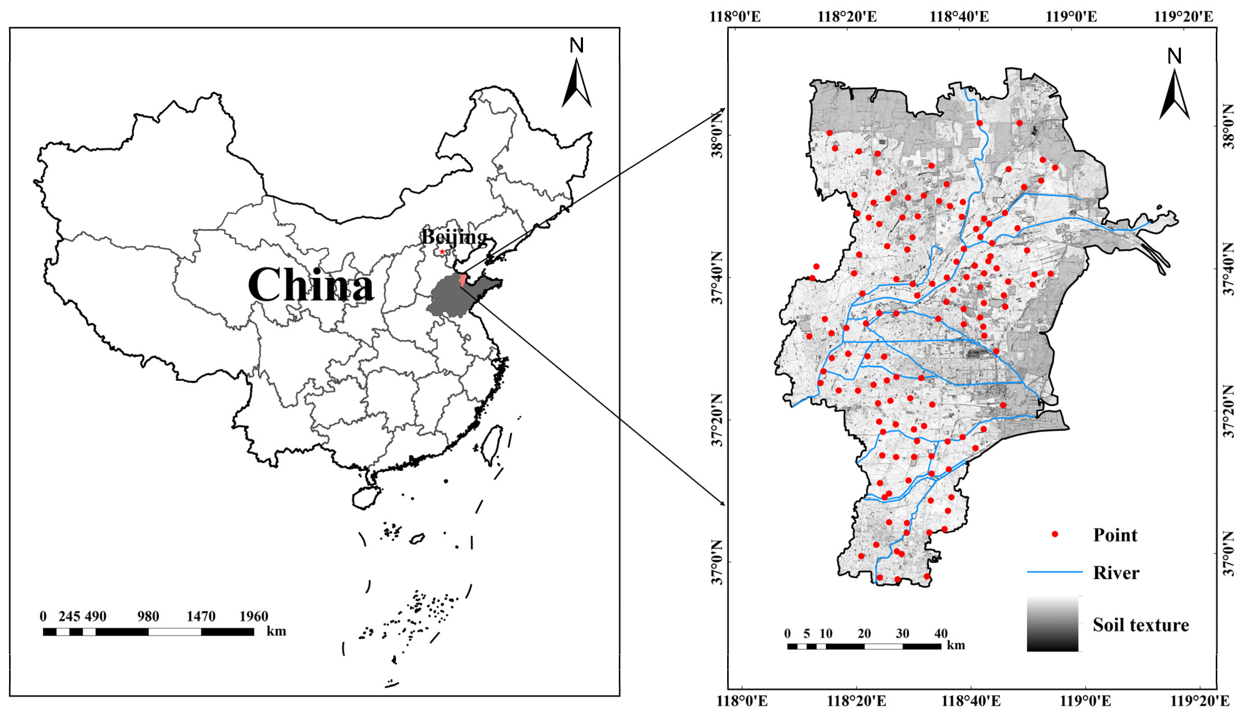
2.1. Study Area

The study area is situated within the Yellow River Delta (YRD) in China (Figure 1) (36°55′–38°10′ N, 118°07′–119°10′ E). The terrain slopes from southwest to northeast along the Yellow River, which belongs to the warm temperate continental monsoon climate. The soil in this region is categorized into five types: cinnamon soil, lime concretion black soil, fluvo-aquic soil, saline soil, and paddy soil. Fluvo-aquic soil is the primary cultivated soil in the study area, which is suitable for wheat, corn, cotton, and other crops. According to the statistical yearbook of Dongying in 2023, the average temperature in the study area is 14.2 °C, the annual precipitation amounts to 794.2 mm, and the annual sunshine hours total 2398.7 h (http://www.dongying.gov.cn/art/2023/10/17/art_38815_10406344.html, (accessed on 1 March 2024)).

2.2. Soil CO₂ Collection

In the farmland of the study area, a total of 133 sampling points were randomly and evenly arranged from 22nd September 2022 to 28th September 2022. Daily measurements of CO₂ flux were taken at 8:00–10:00 a.m. and 3:00–5:00 p.m. The concentration of soil CO₂ flux was ascertained by employing the continuous airflow closure method, and a cylindrical plexiglass chamber (20 cm in diameter and 30 cm in height) was installed in the soil of each sample. The air chamber was inserted into 5 cm of soil, and the air in the glass chamber was connected via a pipe from the air outlet to the pump suction phase velocimeter (FZ2800–2, Guangzhou, China). The measurement interval between sampling points was 10 min, and the initial and final CO₂ contents (unit ppm) were recorded on-site in three parallel measurements. The initial CO₂ content was transformed into the emission flux in accordance with Equation (1) (unit: kg C ha⁻¹ d⁻¹) [24]:

$$\mathit{AE}=c\times v\times 22\times 1440\times {10}^4\times {10}^{-6}/ (\mathit{mv}\times 0.0177)$$

(1)

AE represents the CO₂ volatilization flux, c represents the content of soil CO₂ flux (10⁻³ m mol mol⁻¹) in the pump suction phase speedometer, v represents the airflow velocity (0.25 L min⁻¹), 22 represents the molar mass of CO₂ (g mol⁻¹), 1440 converts min⁻¹ to day⁻¹ (1 d 1440 min), 104 converts m⁻² to ha⁻¹, 10⁻⁶ converts mg C to kg C, mv is the molar volume of CO₂, and 0.0177 is the covered area of the gas chamber (m²).

2.3. Multi-Source Remote Sensing Variables

We selected a diverse array of optical satellite remote sensing data sources, including GF1-WFV, GF6-WFV, GF4-PMI, CB04-MUX, HJ2A-CCD, Sentinel 2-L2A, and Landsat 8-OLI, to furnish comprehensive data support for this research. Among them, the data of GF1-WFV, GF6-WFV, GF4-PMI, CB04-MUX, and HJ2A-CCD come from the China Centre for Resources Satellite Data and Application (https://www.cresda.com/zgzywxyyzx/index.html, (accessed on 1 March 2024)). Sentinel 2-L2A data come from the European Space Agency (https://scihub.copernicus.eu, (accessed on 12 November 2022)), and Landsat 8-OLI data come from the United States Geological Survey (USGS) server (https://earthexplorer.usgs.gov, (accessed on 1 March 2024)). GF4-PMI, CB04-MUX, and HJ2A-CCD satellites transited on 21 September 2022, the Sentinel 2-L2A satellite transited on 23 September 2022, the GF1-WFV satellite transited on 26 September 2022, and the Landsat 8-OLI satellite transited on 28 September 2022. The selection of the time point of the data was carefully considered to ensure that the sampling time is highly consistent with CO₂ and that the influence of interference factors such as cloud coverage is eliminated to the greatest extent. The band and its range and central wavelength and the spatial resolution of the seven kinds of optical satellite remote sensing are shown in

Table 1. Information of seven optical remote sensing satellites.

Image and Resolution (m)	Band Serial Number and Wavelength/Center Wavelength (μm)
GF1-WFV (16)	B1 (0.45–0.52), B2 (0.52–0.59), B3 (0.63–0.69), B4 (0.77–0.89)
GF6-WFV (16)	B1 (0.45–0.52), B2 (0.52–0.59), B3 (0.63–0.69), B4 (0.77–0.89), B5 (0.69–0.73), B6 (0.73–0.77), B7 (0.40–0.45), B8 (0.59–0.63)
GF4-PMI (400)	B2 (0.519), B3 (0.550), B4 (0.628), B5 (0.770)
CB04-MUX (17)	B1 (0.45–0.52), B2 (0.52–0.59), B3 (0.63–0.69), B4 (0.77–0.89)
HJ2A-CCD (30)	B1 (0.485), B2 (0.555), B3 (0.660), B4 (0.830), B5 (0.710)
Sentinel 2-L2A (10)	B1 (0.443), B2 (0.490), B3 (0.560), B4 (0.665), B5 (0.705), B6 (0.740), B7 (0.783), B8 (0.842), B8A (0.865), B9 (0.945), B10 (1.375), B11 (1.610)
Landsat 8-OLI (30)	B1 (0.43–0.45), B2 (0.45–0.51), B3 (0.53–0.59), B4 (0.64–0.67), B5 (0.85–0.88), B6 (1.57–1.65), B7 (2.11–2.29), B9 (1.36–1.38)

. GF1-WFV, GF6-WFV, GF4-PMI, CB04-MUX, and HJ2A-CCD contain the same four bands; the band ranges are 0.45–0.52 μm for the blue band, 0.52–0.59 μm for the green band, 0.63–0.69 μm for the red band, and 0.77–0.89 μm for the near-infrared band. In addition, Landsat 8-OLI has the largest band range, including 12 bands. The band ranges of GF1-WFV and CB04-MUX are narrow, containing only four bands.

2.4. Auxiliary Variables

The remote sensing images of the seven satellites were preprocessed by ENVI 5.6 software through radiation calibration, atmospheric correction, orthorectification, resampling, and cutting of the study area. The resolution was unified to 30 m × 30 m. The vegetation index was a proxy for vegetation conditions by analyzing red, near-infrared, and blue wavelengths to help calculate photosynthetically active radiation (PAR) and carbon fluxes. The vegetation index reveals the spectral characteristics of the vegetation’s ability to absorb and fix CO₂, which affects the monitoring and estimation of soil CO₂ flux. We selected eight vegetation indices to ensure that each satellite could calculate the same vegetation index. Based on the preprocessed images, the band operation tool of ENVI 5.6 software was used to calculate eight vegetation index variables, including the modified chlorophyll absorption in reflectance index (MCARI), triangular vegetation index (TVI), transformed CARI (TCARI), renormalized difference VI (RDVI), green vegetation index (VIgreen), plant senescence reflectance index (PSRI), normalized difference vegetation index (NDVI), and green normalized difference vegetation index (GNDVI) (

Table 2. Vegetation index formulas based on seven remote sensing images.

Index	Formula	Reference
MCARI	$\left(\left(n\mathrm{ir} - \mathrm{re}d\right)- 0.2 \times \left(\mathrm{nir} - \mathrm{green}\right)\right)\times (\mathrm{nir}/\mathrm{red})$	[25]
TVI	$0.5 \times (120 \times (\mathrm{nir} - \mathrm{green}) - 200 \times (\mathrm{red} - \mathrm{green}))$	[26]
TCARI	$3 \times ((\mathrm{nir} - \mathrm{red}) - 0.2 \times (\mathrm{nir} - \mathrm{green}) \times (\mathrm{nir}/\mathrm{red}))$	[27]
RDVI	$(\mathrm{nir} - \mathrm{red})/\sqrt{(\mathrm{nir}+\mathrm{red})}$	[28]
VIgreen	$(\mathrm{green} - \mathrm{red})/(\mathrm{green}+\mathrm{red})$	[29]
PSRI	$(\mathrm{red} - \mathrm{blue})/\mathrm{nir}$	[30]
GNDVI	$(\mathrm{nir} - \mathrm{green})/(\mathrm{nir}+\mathrm{green})$	[31]
NDVI	$(\mathrm{nir} - \mathrm{red})/(\mathrm{nir}+\mathrm{red})$	[32]

).

Based on the raw bands of GF1-WFV (four bands), GF6-WFV (eight bands), GF4-PMI (four bands), CB04-MUX (four bands), HJ2A-CCD (four bands), Sentinel 2-L2A (12 bands), and Landsat 8-OLI (eight bands) remote sensing images, we used ENVI 5.6 software to calculate the gray co-occurrence matrix. Then, eight eigenvalues were extracted, including mean (MEAN), variance (VAR), homogeneity (HOM), contrast (CTRA), dissimilarity (DIS), entropy (ENT), angular second moment (SECM), and correlation (CORR). The eigenvalues of each satellite band and their distribution are shown in Figure 2. GF1-WFV, GF6-WFV, GF4-PMI, CB04-MUX, HJ2A-CCD, Sentinel 2-L2A, and Landsat 8-OLI obtained 32, 64, 32, 32, 40, 96, and 64 texture features, respectively.

In order to retain the original spectral band information and reduce the dimensions of variables, principal component analysis (PCA) was used to reduce the dimensionality of all texture processing results in ENVI 5.6 software. Furthermore, the first three principal components were taken as auxiliary variables for predicting the soil CO₂ flux. The total variance contribution rates of the first three principal components (PCs) of CB04-MUX, GF1-WFV, GF4-PMI, GF6-WFV, HJ2A-CCD, Landsat 8-OLI, and Sentinel 2-L2A images were 91.77%, 99.82%, 93.35%, 87.00%, 86.07%, 97.36%, and 89.21%, respectively (Figure 2). PC1 and PC2 in the seven images typically showed strong aggregation in the visible (VIS) and near-infrared (NIR) bands, and the wavelength range was concentrated within 0.45 to 0.78 μm. The PCs derived from certain satellite images may highlight changes in specific bands to a greater extent than others. PC1 and PC2 of Landsat 8-OLI reflected a broader spectral range, including the shortwave infrared (SWIR) band (1.57–1.65 μm). PC1 and PC2 of GF1-WFV, CB04-MXU, and GF4-PMI were aggregated in the visible light band (0.52–0.55 μm), and PC1 of GF6-WFV had strong loads at B4 (about 0.77–0.89 μm) and B5 (about 0.69–0.73 μm). PC3 of HJ2A-CCD and Sentinel 2-L2A showed a relatively high band-change concentration, mainly concentrated in the short-infrared band (0.83–1.61 μm). PC3 of Landsat 8-OLI was concentrated in the higher short-infrared band range (1.36–2.11 μm).

2.5. Machine Learning

2.5.1. Tree-Structured Parzen Estimator

The tree-structured Parzen estimator (TPE) is a Bayesian-based hyperparameter optimization method [33]. The TPE has good global exploration ability and is not prone to fall into the local optimal state, which makes it suitable for optimizing data with high spatial and temporal variability [34]. Compared with random search methods, the TPE has higher learning efficiency and less suppression by local minima, which enables it to locate the global minima more accurately [35], thus achieving more efficient optimization [36]. The TPE models the conditional probability distribution $p(x|y)$ and the edge probability distribution p(y) and then computes the posterior probability distribution $p(y|x)$ by the Bayesian formula. The TPE uses two density functions to define $p(x|y)$ [33]:

$$p(x|y)=\left\{\begin{array}{c}l(x) if y<y^{*}\hfill \\ g(x) if y\ge y^{*}\hfill \end{array}\right.$$

(2)

l(x) is established using the observation space {x(i)} of the soil CO₂ flux, which corresponds to a loss f(x(i)) less than y *, and g(x) is established using the remaining observations. The TPE uses the expected improvement (EI) as the collection function. Since $p(y|x)$ cannot be obtained, the Bayesian formula is used for the following transformation:

$$E{I}_{y^{*}}(x)={\int }_{-\infty }^{y^{*}}(y^{*}-y)p(y|x)\mathit{dy}={\int }_{-\infty }^{y^{*}}(y^{*}-y){\displaystyle \frac{p(x|y)p(y)}{p(x)}}\mathit{dy}$$

(3)

where y * represents the threshold of soil CO₂ flux. Let γ = p (y < ${y }^{*}$), which represents a certain quantile of the TPE algorithm used to divide l(x) and g(x), and the range is (0, 1). In order to simplify the above formula, the denominator is constructed:

$$p(x)=\int p(x|y)p(y)\mathit{dy}=\gamma l(x)+(1-\gamma )g(x)$$

(4)

Secondly, for molecules, we can obtain

$${\int }_{-\infty }^{y^{*}}(y^{*}-y)p(x|y)p(y)\mathit{dy}=l(x){\int }_{-\infty }^{y^{*}}(y^{*}-y)p(y)\mathit{dy}=\gamma y^{*}l(x)-l(x){\int }_{-\infty }^{y^{*}}p(y)\mathit{dy}$$

(5)

Finally, EI can be simplified to

$$E{I}_{y^{*}}(x)={\displaystyle \frac{\gamma y^{*}l(x)-l(x){\int }_{-\infty }^{y^{*} }p(y)\mathit{dy}}{\gamma l(x)+(1-\gamma )g(x)}}\propto {\left(\gamma +{\displaystyle \frac{g(x)}{l(x)}}(1-\gamma )\right)}^{-1}$$

(6)

To maximize EI, at point x, the probability of l(x) is high, while the probability of g(x) is low. In each iteration, the algorithm returns the candidate x* with the largest EI:

$$x^{*}=\mathit{argmax} E{I}_{y^{*} }(x)$$

(7)

2.5.2. eXtreme Gradient Boosting

The eXtreme gradient boosting (XGBoost) method is a machine learning algorithm based on the gradient tree. On the basis of the gradient boosting decision tree (GDBT), it adds regular terms, including the number of leaf nodes and the sum of the squares of the number of leaf nodes [37]. XGBoost consists of n decision trees, each of which focuses on the residual of the previous tree, and uses a gradient algorithm to find new decision trees [38]. The XGBoost model has the advantage of a lower computational cost than the support vector machine (SVM) model [38]. Compared with the traditional GBDT method, which only uses the first derivative, the XGBoost model performs the second-order Taylor expansion on the loss function, thus making its prediction performance significantly better than the traditional method [39]. XGBoost defines a loss function to minimize the prediction error of the model and designs a regularization function to control the complexity of the model [40], whose objective function ($S^{(t)}$) consists of a loss function and a regularization term. The objective function ($S^{(t)}$) is as follows:

$$S^{(t)}=\sum _{i=1}^{n}L(y_i,{\widehat{y}}_i)+\sum _{k=1}^t\Omega \left(f_k\right)$$

(8)

where $y_i$ is the i-th observed value of soil CO₂ flux, ${\widehat{y}}_i$ is the predicted value at step t (Equation (9)), L and Ω are the loss function the regularization term (Equation (10)), and $f_k$ denotes the k-th tree.

$${\widehat{y}}_i={\sum }_{k=1}^t{f}_k\left(x_i\right)$$

(9)

$$\Omega (f_k)=\gamma T+{\displaystyle \frac{1}{2}} \lambda {\sum }_{j=1}^T{\omega }_j^2$$

(10)

where x_i is the i-th input data point, T represents the total number of nodes in the middle of the decision tree, $\gamma$ represents the complexity of leaf nodes, $\lambda$ is a compromise parameter that measures the penalty, and ${\omega }_j^{ }$ is the fraction on the j-th leaf.

Then, taking k-step optimization as an example, the optimized objective function (Equation (11)) can be approximated by second-order Taylor expansion:

$$S^{\left(t\right)}\cong \sum _{i=1}^n\left[L\left(y_i,{\widehat{y}}_i^{\left(k-1\right)}\right)+g_i{f}_k\left(x_i\right)+{\displaystyle \frac{1}{2}}{h}_i{f}_k^2\left(x_i\right)\right]+\Omega (f_k)$$

(11)

$$g_i={\partial }_{{\widehat{y}}^{\left(t-1\right)}}L\left(y_i,{\widehat{y}}_i^{\left(t-1\right)}\right)$$

(12)

$$h_i={\partial }_{{\widehat{y}}^{\left(t-1\right)}}^2 L\left(y_i,{\widehat{y}}_i^{\left(t-1\right)}\right)$$

(13)

where $g_i$ and $h_i$ are the first and second derivatives of the loss function, respectively, and then the constant term of Equation (11) is removed to obtain the approximate target (Equation (14)):

$$S^{\left(t\right)}=\sum _{i=1}^n\left[g_i{f}_k\left(x_i\right)+{\displaystyle \frac{1}{2}}{h}_i{f}_k^2\left(x_i\right)\right]+\Omega \left(f_k\right)$$

(14)

Then, defining the j-th leaf $I_j=\left\{i\right|q(x_i)=j\}$ as an instance, Equation (14) can be expanded as follows:

$$S^{\left(t\right)}=\sum _{j=1}^T\left[\left(\sum _{i\in I_j}{g}_i\right){\omega }_j+{\displaystyle \frac{1}{2}}\left(\sum _{i\in I_j}{h}_i+\lambda \right){\omega }_j^2\right] +\gamma T$$

(15)

where T represents the total leaf node of the XGBoost model, ω_j and γ represent the score of the j-th leaf and the complexity of the leaf node, respectively, and λ is a compromise parameter to measure the penalty. The core hyperparameters and information of the XGBoost model are shown in

Table 3. Information about the main hyperparameters of the XGBoost model.

Hyperparameters	Type	Range	Explanation
subsample	float	(0.72, 1)	The proportion of random sampling per tree
num_boost_round	int	(50, 500)	The number of boosting iterations during the training process
eta	float	(0.04, 0.36)	The learning rate
lambda	float	(0, 7)	The regularization part of XGBoost processing
min_child_weight	float	(1.2, 4.8)	The sum of weights of the minimum leaf node sample
colsample_bytree	float	(0.72, 1)	The proportion of features used for training to all features
colsample_bynode	float	(0.72, 1)	The subsampling rate of each node split column
max_depth	int	(2, 9)	The maximum depth of a tree

.

2.6. Verification

In this study, 133 samples were randomly divided into a training set with 70% of the data and a testing set with 30% to build prediction models for the seven types of satellites. The root-mean-square error (RMSE) (Equation (16)) and coefficient of determination (R²) (Equation (17)) were used to evaluate the accuracy of different satellites:

$$\mathrm{RMSE}=\sqrt{{\displaystyle \frac{1}{\mathrm{n}}}\sum _{\mathrm{i}=1}^{\mathrm{n}}{(\widehat{p}({\mathrm{x}}_{\mathrm{i}}) - p({\mathrm{x}}_{\mathrm{i}}))}^2}$$

(16)

$${\mathrm{R}}^2={\left[{\displaystyle \frac{{\sum }_{\mathrm{i}=1}^{\mathrm{n}}\left(p({\mathrm{x}}_{\mathrm{i}}) -\overline{p({\mathrm{x}}_{\mathrm{i}})}\right)\left(\widehat{p}({\mathrm{x}}_{\mathrm{i}}) -\overline{\widehat{p}({\mathrm{x}}_{\mathrm{i}})}\right)}{\sqrt{{\sum }_{\mathrm{i}=1}^{\mathrm{n}}{\left(p({\mathrm{x}}_{\mathrm{i}}) -\overline{p({\mathrm{x}}_{\mathrm{i}})}\right)}^2{\left(\widehat{p}({\mathrm{x}}_{\mathrm{i}}) - \overline{\widehat{p}({\mathrm{x}}_{\mathrm{i}})}\right)}^2}}}\right]}^2$$

(17)

$\widehat{p}(x_i)$ and $p(x_i)$ are the true and predicted values of soil carbon dioxide content, respectively, and $\overline{p(x_i)}$ and $\overline{\widehat{p}(x_i)}$ are the average values of the true values of soil carbon dioxide content and the average values of the model estimates at 133 sample points, respectively.

2.7. SHAP Analysis

SHapley additive explanations (SHAP) is a method for explaining machine learning model predictions based on SHapley value theory in cooperative game theory. SHAP determines how much each feature contributes to the results by calculating the contribution of each feature to the predicted results of different combinations [41]. Compared with traditional interpretation methods, SHAP provides a clear visualization of the influence of individual features in the sample prediction on the prediction results, thus improving the global interpretability of the targets [42]. SHAP is widely used to interpret various machine learning models to help users understand the model’s predictive process. The SHapley value can be regarded as the contribution of the feature to the difference between the actual prediction (including x_i) and the average prediction (without x_i). $f(S\cup \{x_i\})-f(S)$ can represent the marginal contribution of x_i. The calculation of SHAP values involves evaluating all subsets of the feature space, and the specific formula is as follows [35]:

$${\varphi }_i(f,x)={\displaystyle \frac{1}{N!}}\sum _{S\subseteq p\backslash x_i}\left[\right|S|!(N-\left|S\right|-1)!\left]\right[f(S\cup \{x_i\})-f(S)]$$

(18)

x is the input feature, N is the number of input features in x, f is the original prediction model, ${\varphi }_i$ is the attribution factor (SHapley value), P is all the eigenvalues set, S is the feature subset of the model excluding the eigenvalue $x_i$, and $\left|S\right|$ is the number of non-zero items in S. In this study, based on the SHAP results of a single satellite, the first two important variables of each satellite were selected to form auxiliary variables for the multi-satellite collaborative prediction of soil CO₂ flux.

3. Results

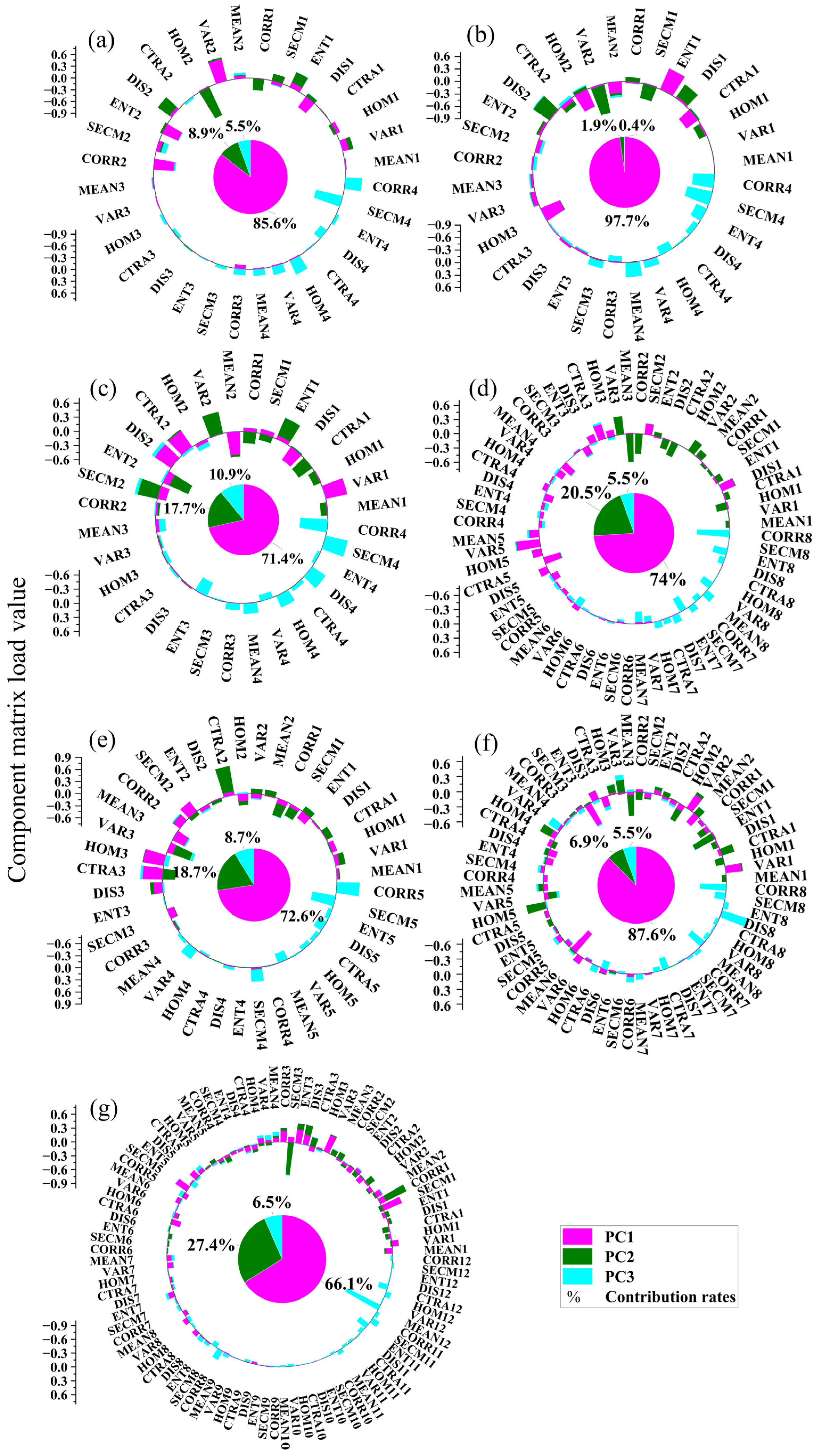
3.1. Statistical Analysis

Figure 3 shows the normalized numerical distribution of soil CO₂ fluxes and other auxiliary variables in each single-satellite image data source. Among the variables of these satellites, only the numerical distributions of PC1 of CB04-MUX and soil CO₂ flux were similar, which exhibited left-skewed distributions. The distribution trends of soil texture variables of different satellites were left-skewed (i.e., PC1 of HJ2A-CCD and PC2 of GF6-WFV) or right-skewed (i.e., PC1 of GF1-WFV, GF6-WFV, and Landsat 8-OLI, and PC2 of GF4-PMI). The TVI values of all satellites were consistent and close to a normal distribution. Similarly, the VIgreen values of most satellites (except Sentinel 2-L2A) also showed significant normality. The numerical distribution trends of MCARI and TCARI in GF1-WFV, GF6-WFV, Landsat 8-OLI, and Sentinel 2-L2A were similar, all exhibiting a left-skewed distribution. Conversely, the numerical distributions of other index variables across different satellites exhibited complex distribution characteristics. The numerical distribution characteristics of the above variables indicate that different satellites are affected by weather conditions and land cover, resulting in the complexity of soil texture and vegetation index variables. That is, it is difficult to use the auxiliary variables of a single satellite for the nonlinear spatial prediction of soil CO₂ flux.

Among the vegetation index variables, different satellite data demonstrate some common linear correlation patterns. The positive correlations between MCARI and TCARI, RDVI and GNDVI, and NDVI and GNDVI were high across multiple datasets (r ≥ 0.80). However, the negative correlation between VIgreen and PSRI was higher in some datasets (r ≤ −0.50). The correlation among soil texture variables is more complex, with a positive correlation between PC2 and PC3 of GF6-WFV (r = 0.78) and a negative linear correlation between PC1 and PC3 of GF1-WFV (r = −0.60). In addition, positive correlations between soil CO₂ flux and vegetation indices (i.e., MCARI and TCARI from the CB04-MUX data) (r = 0.20) and soil texture (PC1 and PC2 from the Sentinel 2-L2A data) (r = 0.14 and r = 0.16) were obvious, and the negative correlation between soil CO₂ flux and PC1 was obvious in HJ2A-CCD data (r = −0.17). It is notable that the linear relationships between soil CO₂ fluxes and single-satellite environmental variables are generally weak, which may indicate that soil CO₂ flux predictions need to take into account more satellite data.

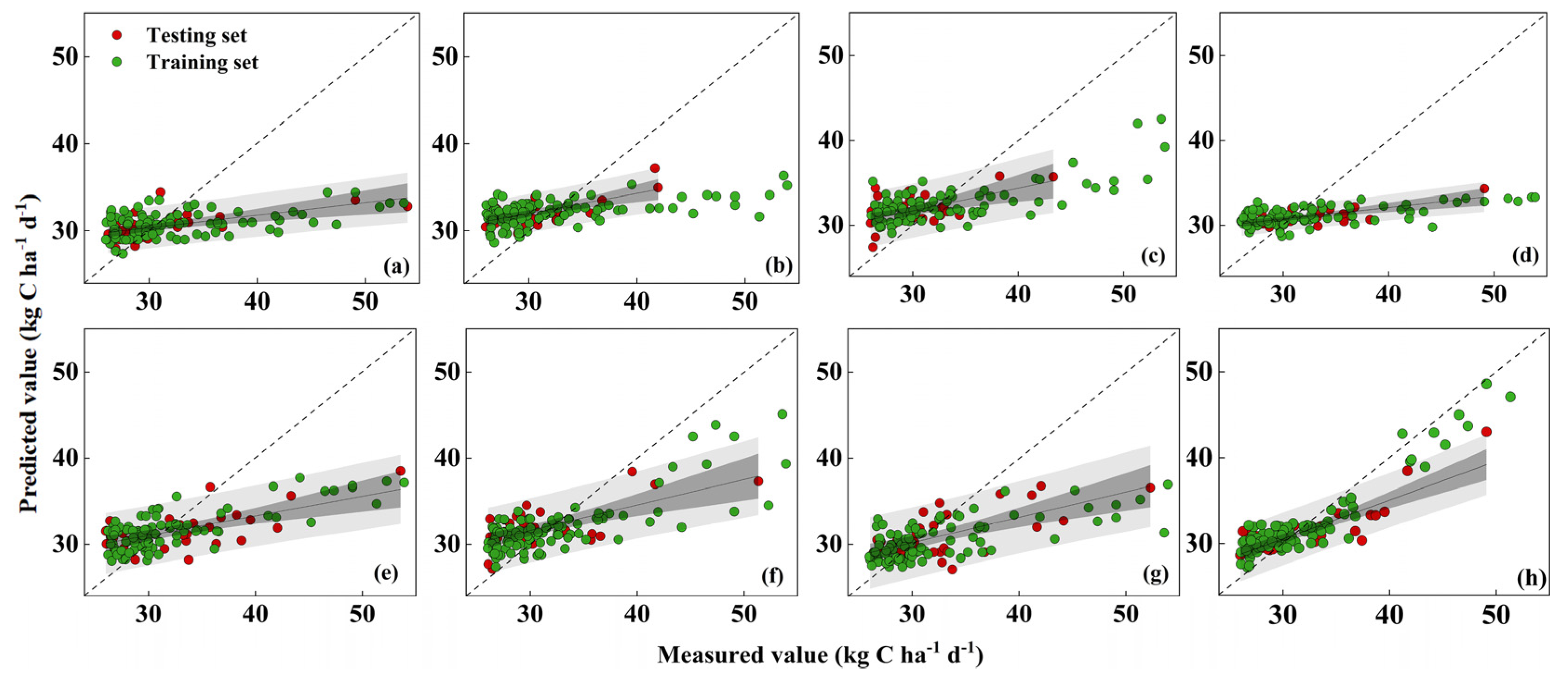
3.2. Accuracy Evaluation of Single-Satellite Prediction

Table 4. Prediction accuracy of soil CO₂ flux using TPE-XGBoost model.

		STD (kg C ha−1 d−1)	RMSE (kg C ha−1 d−1)	R²
GF1-WFV	Testing set	1.36	3.46	0.41
	Training set	1.33	6.27	0.28
GF6-WFV	Testing set	0.90	3.94	0.45
	Training set	1.03	6.34	0.36
GF4-PMI	Testing set	1.77	3.49	0.29
	Training set	2.20	5.51	0.50
CB04-MUX	Testing set	1.39	5.15	0.36
	Training set	1.43	6.11	0.22
HJ2A-CCD	Testing set	2.14	5.10	0.42
	Training set	2.22	4.90	0.57
Sentinel 2-L2A	Testing set	2.59	4.87	0.45
	Training set	2.16	5.42	0.47
Landsat 8-OLI	Testing set	2.31	4.12	0.43
	Training set	3.17	4.57	0.62
All	Testing set	2.75	3.23	0.73
	Training set	4.09	2.29	0.87

shows the prediction accuracy of soil CO₂ flux from a single-satellite image based on the TPE-XGBoost model. Compared with other satellites, Landsat 8-OLI (R² = 0.43), Sentinel 2-L2A (R² = 0.45), and HJ2A-CCD (R² = 0.42) had higher prediction accuracy on the testing set, indicating that the auxiliary variables of these satellites had a strong fitting ability for the soil CO₂ flux. The testing set prediction accuracy of GF6-WFV (R² = 0.45), CB04-MUX (R² = 0.36), and GF1-WFV (R² = 0.41) satellites was higher than that on the training set. This shows that the auxiliary variables extracted by these satellites have poor adaptability to the prediction model. Interestingly, even though HJ2A-CCD, Sentinel 2-L2A, and Landsat 8-OLI exhibited high fitting capabilities (R²), their RMSEs were higher than those of other satellites. In other words, there is high uncertainty in the prediction of soil CO₂ flux by a single satellite, indicating that the auxiliary variables extracted by the same satellites have mutual inhibition. This phenomenon is also reflected in the scatter plot. Figure 4 shows the scatter comparison of predicted and measured soil CO₂ fluxes from the seven satellites. Compared with other satellites, GF6-WFV had a more compact scatter distribution and fewer extreme values. The seven types of satellites generally overestimated the CO₂ flux in the low-value region, and there was an underestimation of the measured soil CO₂ flux when the value was above 32 kg C ha⁻¹ d⁻¹. The dispersion of the single satellite is far away from the 1:1 diagonal, and the residual value is high, which indicates the weak nonlinear interpretation ability for the soil CO₂ flux.

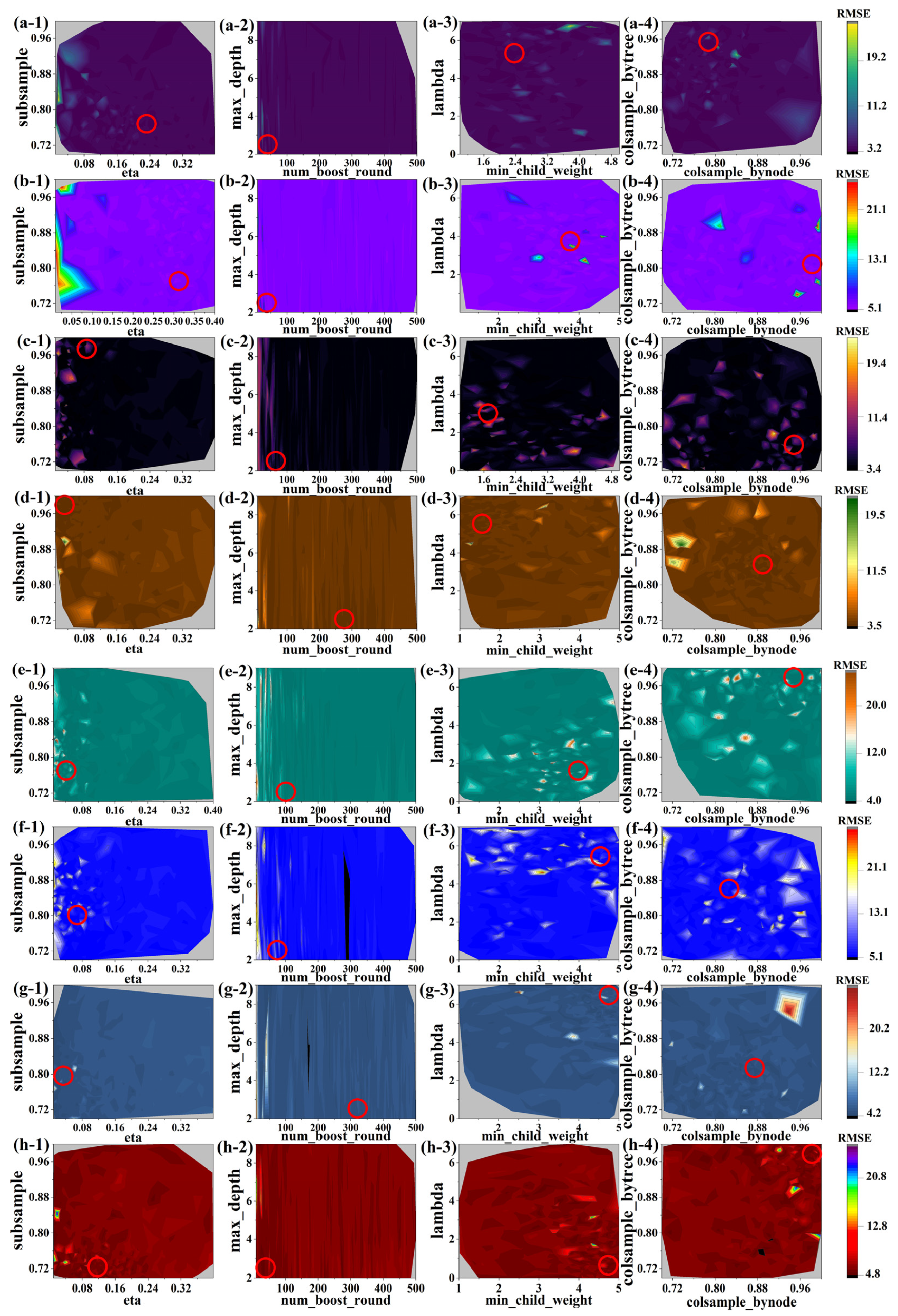
3.3. Hyperparameter Optimization

The hyperparameters of the XGBoost model with multi-satellite and single-satellite data are optimized by the TPE algorithm. Figure 5 shows the iterative trend of RMSE during TPE optimization. Obviously, the iterations in TPE optimization have a tendency for sparsity and aggregation. In each hyperparameter iteration process, there is a region with the densest iteration sample points (such as num_boost_round (0–100) and eta (0–0.10)). There are significant differences between the densely sampled areas and the sparsely sampled areas, and the optimal parameters tend to appear near the densely sampled areas. This is because the TPE always selects the next sampling point on the basis of the previous iteration to approximate the optimal parameter. After multiple iterations, the probability of the optimal hyperparameter appearing in the densely sampled region is much higher than that in the sparsely sampled region. The iterative sampling points of the hyperparameter num_boost_round are distributed in a banded manner, while the sampling points of other hyperparameters (such as min_child_weight and colsample_bynode) are clustered in a patchy manner. In addition, the minimum RMSE distributions of different satellite data for the same hyperparameter are different. During the iterative process of eta, subsample, and num_boost_round, the minimum RMSE distribution of most satellite data is relatively concentrated, especially in the 0–100 region of num_boost_round. However, in the max_depth iteration, the lowest RMSE for all satellite data appeared in the two-to-three region, showing high consistency. For other hyperparameters (such as min_child_weight and lambda), the minimum RMSE distribution of different satellite data is more dispersed, covering several different numerical regions.

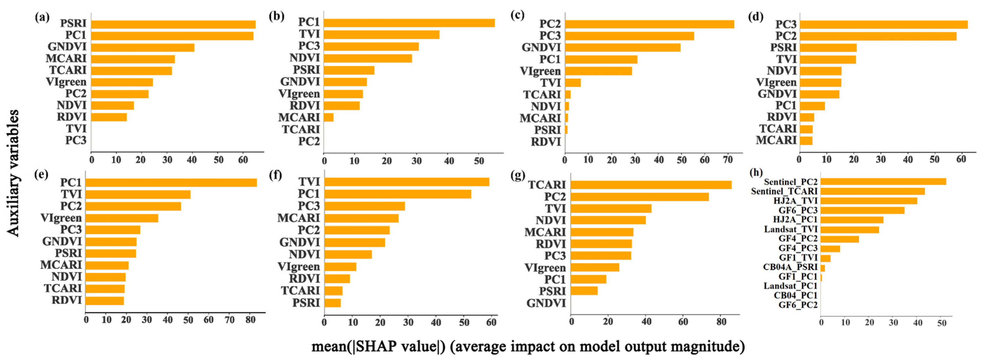
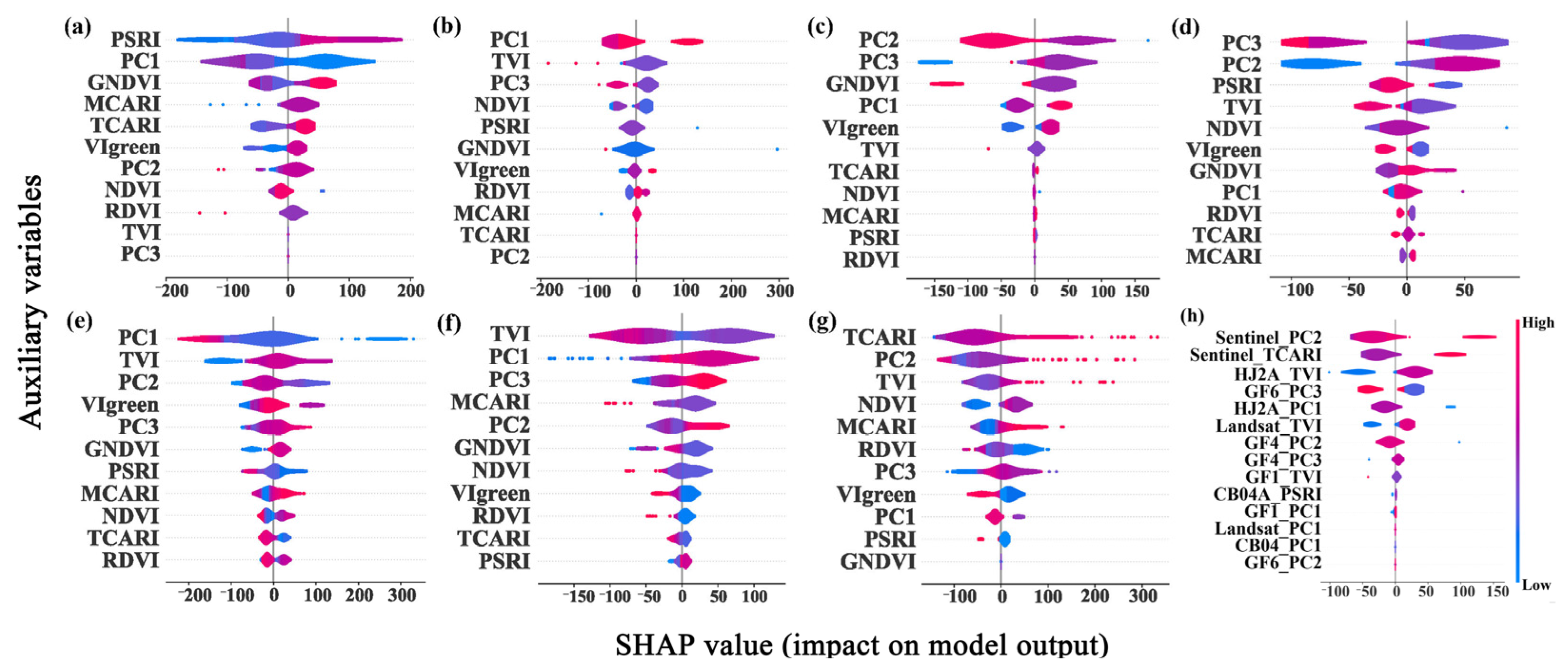
3.4. Variable Importance

Figure 6 shows the variable importance of single-satellite data for the prediction of soil CO₂ flux based on SHAP analysis. Soil texture characteristics exhibited significant importance in the prediction of soil CO₂ flux. PC1 of CB04-MUX, GF1-WFV, HJ2A-CCD, and Landsat 8-OLI data and PC2 and PC3 of GF4-PMI and GF6-WFV data had the highest driving force for the prediction accuracy of CO₂ flux. In the CB04-MUX and HJ2A-CCD satellites, PC1 had a significant negative driving effect on soil CO₂ flux, while PC1 of the GF1-WFV and Landsat 8-OLI data was positive (Figure 7). Similarly, PC2 of GF4-PMI and PC3 of GF6-WFV were negative drivers for soil CO₂ flux, while PC3 of GF4-PMI and PC2 of GF6-WFV were positive.

As another key variable, the vegetation index also plays a significant role in the prediction of soil CO₂ flux. The contributions of the TVI of GF1-WFV, HJ2A-CCD, and Landsat 8-OLI, as well as the PSRI and TCARI of CB04-MUX and Sentinel 2-L2A, to the prediction accuracy of soil CO₂ flux were relatively high. Other index variables, such as the GNDVI, MCARI, VIgreen, NDVI, and RDVI, had a weak driving force. The TVI of GF1-WFV and Landsat 8-OLI data had a negative driving effect on the prediction of soil CO₂ flux, while the TVI of HJ2A-CCD was positive. In CB04-MUX and Sentinel 2-L2A, the PSRI and TCARI had significant positive driving effects on soil CO₂ flux, while other indices, such as the GNDVI, MCARI, and VIgreen, had weak driving effects.

3.5. Multi-Satellite Prediction Accuracy and Variable Importance

Based on the SHAP results of a single satellite, the first two important auxiliary variables of each satellite were selected to predict the soil CO₂ flux based on the TPE-XGBoost model. Compared with the prediction accuracy of the single-satellite data, the prediction accuracy of the multi-satellite auxiliary variables for soil CO₂ flux was higher (RMSE = 3.23 kg C ha⁻¹ d⁻¹ and R² = 0.73). Furthermore, the difference between the training set and the testing set of the multi-satellite auxiliary variables is small, indicating that the auxiliary variables from multi-satellite data have a stronger ability to explain the spatial variability of soil CO₂ flux. Figure 4 shows the scatter comparison of predicted and measured soil CO₂ fluxes from multi-satellite data. The soil CO₂ flux predicted by multi-satellite auxiliary variables showed an overestimation in the low-value region, but the scatter points in the high-value region were closer to the diagonal, and the underestimation was not significant.

The driving effects of multiple-satellite auxiliary variables on soil CO₂ flux are presented in Figure 6. Among all of the variables, PC2 of Sentinel 2-L2A data had the greatest impact on the prediction accuracy of soil CO₂ flux, followed by the TCARI of Sentinel 2-L2A data, the TVI of HJ2A-CCD data, and PC3 of GF6-WFV data. Other variables, such as PC1 of HJ2A-CCD data and the TVI of Landsat 8-OLI data, had a relatively minor influence on the prediction accuracy of soil CO₂ flux. Additionally, PC2 and the TCARI of Sentinel 2-L2A data, as well as the TVI of HJ2A-CCD data, had significant positive driving effects on the prediction accuracy of soil CO₂ flux, whereas PC3 and PC1 of GF6-WFV and HJ2A-CCD data had negative effects.

3.6. The Spatial Mapping of Soil CO₂ Flux Using the TPE-XGBoost Model

The TPE-XGBoost model was used to map soil CO₂ flux in the study area. The mapping results of the model were close to the range of the actual sampling data (Figure 8), which demonstrated the powerful ability of the model to predict the soil CO₂ flux in nonlinear space with multi-source remote sensing variables. The mapping results showed that the high CO₂ flux in the soil was mainly concentrated in farmland near the eastern cities, which may be related to urban expansion and intensive agricultural activities. The northern saline-alkali lands and the areas near rivers also showed higher soil CO₂ flux, while the southern and western regions showed lower soil CO₂ flux. The spatial distribution of soil CO₂ flux in farmland in the study area has significant complexity and heterogeneity. It is influenced not only by natural geographical variables (such as soil type and hydrological conditions) but also by human activities (such as the urbanization process and agricultural management methods).

4. Discussion

4.1. Effects of Auxiliary Variables on Soil CO₂ Flux

In this study, the soil texture characteristics represented by soil texture (i.e., PC1, PC2, and PC3) had a significant impact on soil CO₂ flux. Soil texture regulates soil CO₂ flux by influencing physical variables such as soil moisture, soil temperature, and soil pressure. The soil types in the study area include aquic soil, paddy soil, loamy soil, and clay soil. Compared with sandy soil, the soil loses less water [43] and the soil is wetter, resulting in increased CO₂ flux from the soil [44]. Soil texture also affects soil temperature [45]. Warmer soil usually has a higher rate of soil CO₂ flux [46]. The study area is saline-alkali land, and the intensification of soil salinization will make the surface prone to erosion [47], and high pressure will increase the soil CO₂ flux at these erosion sites [48]. High erosion causes the instability of soil aggregates, increases the exposure of SOC to microbial decomposition, and promotes the production of more CO₂ from SOC consumption [49].

In addition to soil texture, vegetation also had a significant effect on the spatial variation in soil CO₂ flux. Vegetation indices such as the NDVI directly affect the soil CO₂ flux [46] through the growth status and productivity of vegetation (vegetation cover, root function, and transpiration). Vegetation absorbs CO₂ from the atmosphere through photosynthesis [50] and releases CO₂ back to the soil through root respiration [51], affecting the carbon cycle of the soil. Areas with high vegetation coverage tend to have higher rates of soil CO₂ flux [52,53,54]. High vegetation coverage not only provides a rich carbon source for the soil [54] but also promotes the growth and metabolism of microorganisms by improving the soil environment (such as humidity and temperature) [51,55]. This increases the release of CO₂. In addition, with high vegetation coverage [46], root respiration will be enhanced, promoting soil CO₂ flux. These findings are consistent with the positive driving effects of vegetation indices such as the TVI on soil CO₂ flux in this study and emphasize the key role of vegetation in regulating soil CO₂ flux. Moreover, human activities, such as the use of chemical fertilizers, also affect soil CO₂ flux. Fertilization can increase organic carbon storage [56] and contribute significantly to soil CO₂ flux [57].

4.2. Limitations

In this study, a variety of remote sensing satellite images combined with the TPE-XGBoost model were used to predict and map the soil CO₂ flux in farmland soil in the YRD of China. It is evident that the multi-source remote sensing strategy can enhance the spatial prediction accuracy of soil CO₂ flux. However, there are still some limitations in this study that need to be explored in future studies. First, due to the limited access to data and the high cost of inputs, this study failed to achieve the full coverage of remote sensing image types, especially hyperspectral data. As a result of the failure to utilize the finer and richer spectral information provided by hyperspectral images, the ability of hyperspectral bands to respond to soil CO₂ flux cannot be explored more deeply. Second, there are significant differences in the number of wavelengths and bands between different images. This difference leads to some vegetation indices (such as those calculated based on the red-edge band of the Sentinel image) being overlooked in order to maintain the same vegetation index. The absence of these indices may limit the in-depth understanding of the complex relationship between vegetation and soil CO₂ flux. Third, the collection time of soil CO₂ flux was in September, and there was a lack of continuous multi-season observation data. Since seasonal changes in climate and vegetation growth conditions have significant effects on soil CO₂ flux, it is difficult for studies to fully assess changes on broader time and spatial scales with data from a single season. Fourth, this study only sampled farmland ecosystems and ignored the soil CO₂ flux of other important ecosystem types, such as wetland, forest land, and grassland, in the YRD. The uniformity of this sampling type may lead to limitations in the generalization of the study results to other ecosystems, which cannot fully reflect the characteristics of soil CO₂ flux at regional scales. Since different ecosystems play different roles in the process of CO₂ absorption and flux, the relationship between them is of great significance for the accurate assessment of regional carbon balance and ecological environment. In addition, there are many variables affecting soil CO₂ flux. Climatic variables such as solar radiation, air temperature, and soil moisture also have a certain impact on soil CO₂ flux. Due to their numerousness and complexity, environmental variables have different influences on soil CO₂ flux, so climate variables such as solar radiation were not considered in this article.

Therefore, hyperspectral remote sensing data should be actively introduced in future studies so as to more comprehensively and accurately investigate the spatio-temporal variation characteristics of soil CO₂ flux. Combining multi-temporal remote sensing data to make spatio-temporal predictions is the key to further improving the prediction accuracy in future studies. Accordingly, CO₂ flux data from multiple seasons should be taken into consideration in the future and combined with multi-temporal remote sensing data to reveal the spatio-temporal variability of CO₂ flux. At the same time, subsequent studies should build a comprehensive monitoring network for soil CO₂ flux in wetland, forest, and grassland ecosystems in the YRD so as to improve the universality of soil CO₂ flux prediction models in various soil utilization types. In addition, the complex relationship between environmental variables and soil CO₂ will be further explored in future studies so as to provide a more comprehensive and accurate scientific basis for regional agricultural sustainable development and response to climate change.

5. Conclusions

In this study, multi-source satellite remote sensing data were employed to improve the spatial prediction accuracy of soil CO₂ flux. The optimal hyperparameters were obtained from the XGBoost model optimized by the TPE algorithm, and it was discovered that the optimal hyperparameters often appear in the dense sampling area during TPE iteration. There is a complex linear relationship between the soil texture and vegetation indices of different satellite data and soil CO₂ flux. Compared with single-satellite prediction, the multi-source satellite data model combined with TPE-XGBoost demonstrates a superior capability to explain the spatial variability of soil CO₂ flux. The high soil CO₂ flux in farmland in the study area is mainly concentrated in eastern and northern farmlands. Vegetation indices and soil texture characteristics have significant positive driving effects on the prediction accuracy of soil CO₂ flux. The photosynthesis and root respiration of vegetation, as well as the regulating effect of soil texture on water and temperature, jointly promoted soil CO₂ flux in farmland in the study area. That is to say, increases in soil moisture and temperature promote microbial activity and accelerate the decomposition of organic carbon, thus increasing the soil CO₂ flux. In the future, we can delve into changes in the complex relationship between auxiliary variables and soil CO₂ flux in different geographical regions and seasons. This will contribute to a deeper understanding of the spatial and temporal distributions of soil CO₂ flux and its driving mechanism and contribute to the mitigation of regional climate warming and the promotion of sustainable agricultural development.

References

1. Change, On Climate. Intergovernmental panel on climate change. World Meteorol. Organ. 2007, 52, 1–43.
2. Fan, R.; Zhang, B.; Li, J.; Zhang, Z.; Liang, A. Straw-derived biochar mitigates CO2 emission through changes in soil pore structure in a wheat-rice rotation system. Chemosphere 2020, 243, 125329. [Google Scholar] [CrossRef]
3. Forte, A.; Fiorentino, N.; Fagnano, M.; Fierro, A. Mitigation impact of minimum tillage on CO2 and N2O emissions from a Mediterranean maize cropped soil under low-water input management. Soil. Till. Res. 2017, 166, 167–178. [Google Scholar] [CrossRef]
4. De Stefano, A.; Jacobson, M.G. Soil carbon sequestration in agroforestry systems: A meta-analysis. Agroforest. Syst. 2018, 92, 285–299. [Google Scholar] [CrossRef]
5. Deng, Y.; He, Z.; Xiong, J.; Yu, H.; Xu, M.; Hobbie, S.E.; Reich, P.B.; Schadt, C.W.; Kent, A.; Pendall, E. Elevated carbon dioxide accelerates the spatial turnover of soil microbial communities. Glob. Chang. Biol. 2016, 22, 957–964. [Google Scholar] [CrossRef]
6. Okubo, T.; Liu, D.; Tsurumaru, H.; Ikeda, S.; Asakawa, S.; Tokida, T.; Tago, K.; Hayatsu, M.; Aoki, N.; Ishimaru, K. Elevated atmospheric CO2 levels affect community structure of rice root-associated bacteria. Front. Microbiol. 2015, 6, 136. [Google Scholar] [CrossRef]
7. Takahashi, A.; Hiyama, T.; Takahashi, H.A.; Fukushima, Y. Analytical estimation of the vertical distribution of CO2 production within soil: Application to a Japanese temperate forest. Agr. Forest Meteorol. 2004, 126, 223–235. [Google Scholar] [CrossRef]
8. Hannam, K.D.; Midwood, A.J.; Neilsen, D.; Forge, T.A.; Jones, M.D. Bicarbonates dissolved in irrigation water contribute to soil CO2 efflux. Geoderma 2019, 337, 1097–1104. [Google Scholar] [CrossRef]
9. Camarda, M.; De Gregorio, S.; Capasso, G.; Di Martino, R.M.R.; Gurrieri, S.; Prano, V. The monitoring of natural soil CO2 emissions: Issues and perspectives. Earth-Sci. Rev. 2019, 198, 102928. [Google Scholar] [CrossRef]
10. Scudero, S.; D’Alessandro, A.; Giuffrida, G.; Gurrieri, S.; Liuzzo, M. Wavelet-based filtering and prediction of soil CO2 flux: Example from Etna volcano (Italy). J. Volcanol. Geoth. Res. 2022, 421, 107421. [Google Scholar] [CrossRef]
11. Gebremichael, A.; Orr, P.J.; Osborne, B. The impact of wetting intensity on soil CO2 emissions from a coastal grassland ecosystem. Geoderma 2019, 343, 86–96. [Google Scholar] [CrossRef]
12. Breiman, L. Random forests. Mach. Learn. 2001, 45, 5–32. [Google Scholar] [CrossRef]
13. Bregaglio, S.; Mongiano, G.; Ferrara, R.M.; Ginaldi, F.; Lagomarsino, A.; Rana, G. Which are the most favourable conditions for reducing soil CO2 emissions with no-tillage? Results from a meta-analysis. Int. Soil Water Conse. 2022, 10, 497–506. [Google Scholar] [CrossRef]
14. Andrews, H.M.; Homyak, P.M.; Oikawa, P.Y.; Wang, J.; Jenerette, G.D. Water-conscious management strategies reduce per-yield irrigation and soil emissions of CO2, N2O, and NO in high-temperature forage cropping systems. Agr. Ecosyst. Environ. 2022, 332, 107944. [Google Scholar] [CrossRef]
15. Song, X.; Wang, G.; Ran, F.; Chang, R.; Song, C.; Xiao, Y. Effects of topography and fire on soil CO2 and CH4 flux in boreal forest underlain by permafrost in northeast China. Ecol. Eng. 2017, 106, 35–43. [Google Scholar] [CrossRef]
16. Crabbe, R.A.; Janouš, D.; Dařenová, E.; Pavelka, M. Exploring the potential of LANDSAT-8 for estimation of forest soil CO2 efflux. Int. J. Appl. Earth Obs. 2019, 77, 42–52. [Google Scholar] [CrossRef]
17. Huang, N.; Gu, L.; Black, T.A.; Wang, L.; Niu, Z. Remote sensing-based estimation of annual soil respiration at two contrasting forest sites. J. Geophys. Res. Biogeo. 2015, 120, 2306–2325. [Google Scholar] [CrossRef]
18. Wu, C.; Gaumont-Guay, D.; Black, T.A.; Jassal, R.S.; Xu, S.; Chen, J.M.; Gonsamo, A. Soil respiration mapped by exclusively use of MODIS data for forest landscapes of Saskatchewan, Canada. ISPRS J. Photogramm. 2014, 94, 80–90. [Google Scholar] [CrossRef]
19. Huang, N.; Gu, L.; Niu, Z. Estimating soil respiration using spatial data products: A case study in a deciduous broadleaf forest in the Midwest USA. J. Geophys. Res. Atmos. 2014, 119, 6393–6408. [Google Scholar] [CrossRef]
20. Gao, Y.; Yu, G.; Li, S.; Yan, H.; Zhu, X.; Wang, Q.; Shi, P.; Zhao, L.; Li, Y.; Zhang, F. A remote sensing model to estimate ecosystem respiration in Northern China and the Tibetan Plateau. Ecol. Model. 2015, 304, 34–43. [Google Scholar] [CrossRef]
21. Valerio, A.M.; Kampel, M.; Ward, N.D.; Sawakuchi, H.O.; Cunha, A.C.; Richey, J.E. CO2 partial pressure and fluxes in the Amazon River plume using in situ and remote sensing data. Cont. Shelf Res. 2021, 215, 104348. [Google Scholar] [CrossRef]
22. Chen, X.; He, Q.; Ye, T.; Liang, Y.; Li, Y. Decoding spatiotemporal dynamics in atmospheric CO2 in Chinese cities: Insights from satellite remote sensing and geographically and temporally weighted regression analysis. Sci. Total Environ. 2024, 908, 167917. [Google Scholar] [CrossRef]
23. Gong, W.; Huang, C.; Houghton, R.A.; Nassikas, A.; Zhao, F.; Tao, X.; Lu, J.; Schleeweis, K. Carbon fluxes from contemporary forest disturbances in North Carolina evaluated using a grid-based carbon accounting model and fine resolution remote sensing products. Sci. Remote Sens. 2022, 5, 100042. [Google Scholar] [CrossRef]
24. Thottathil, S.D.; Reis, P.C.; Prairie, Y.T. Magnitude and drivers of oxic methane production in small temperate lakes. Environ. Sci. Technol. 2022, 56, 11041–11050. [Google Scholar] [CrossRef]
25. Daughtry, C.S.; Walthall, C.L.; Kim, M.S.; De Colstoun, E.B.; McMurtrey Iii, J.E. Estimating corn leaf chlorophyll concentration from leaf and canopy reflectance. Remote Sens. Environ. 2000, 74, 229–239. [Google Scholar] [CrossRef]
26. Broge, N.H.; Leblanc, E. Comparing prediction power and stability of broadband and hyperspectral vegetation indices for estimation of green leaf area index and canopy chlorophyll density. Remote Sens. Environ. 2001, 76, 156–172. [Google Scholar] [CrossRef]
27. Haboudane, D.; Miller, J.R.; Tremblay, N.; Zarco-Tejada, P.J.; Dextraze, L. Integrated narrow-band vegetation indices for prediction of crop chlorophyll content for application to precision agriculture. Remote Sens. Environ. 2002, 81, 416–426. [Google Scholar] [CrossRef]
28. Roujean, J.; Breon, F. Estimating PAR absorbed by vegetation from bidirectional reflectance measurements. Remote Sens. Environ. 1995, 51, 375–384. [Google Scholar] [CrossRef]
29. Gitelson, A.A.; Kaufman, Y.J.; Stark, R.; Rundquist, D. Novel algorithms for remote estimation of vegetation fraction. Remote Sens. Environ. 2002, 80, 76–87. [Google Scholar] [CrossRef]
30. Fernández-Manso, A.; Fernández-Manso, O.; Quintano, C. SENTINEL-2A red-edge spectral indices suitability for discriminating burn severity. Int. J. Appl. Earth Obs. 2016, 50, 170–175. [Google Scholar] [CrossRef]
31. Gitelson, A.A.; Merzlyak, M.N. Signature analysis of leaf reflectance spectra: Algorithm development for remote sensing of chlorophyll. J. Plant Physiol. 1996, 148, 494–500. [Google Scholar] [CrossRef]
32. Rouse, J.W.; Haas, R.H.; Schell, J.A.; Deering, D.W.; Harlan, J.C. Monitoring the Vernal Advancements and Retrogradation; Texas A & M University: College Station, TX, USA, 1974. [Google Scholar]
33. Putatunda, S.; Rama, K. A comparative analysis of hyperopt as against other approaches for hyper-parameter optimization of XGBoost. In Proceedings of the 2018 International Conference on Signal Processing and Machine Learning, Shanghai, China, 28–30 November 2018; pp. 6–10. [Google Scholar]
34. Yu, J.; Zheng, W.; Xu, L.; Meng, F.; Li, J.; Zhangzhong, L. TPE-CatBoost: An adaptive model for soil moisture spatial estimation in the main maize-producing areas of China with multiple environment covariates. J. Hydrol. 2022, 613, 128465. [Google Scholar] [CrossRef]
35. Chen, C.; Seo, H. Prediction of rock mass class ahead of TBM excavation face by ML and DL algorithms with Bayesian TPE optimization and SHAP feature analysis. Acta Geotech. 2023, 18, 3825–3848. [Google Scholar] [CrossRef]
36. Maurice, C.; Madrigal, F.; Lerasle, F. Hyper-optimization tools comparison for parameter tuning applications. In Proceedings of the 2017 14th IEEE International Conference on Advanced Video and Signal Based Surveillance (AVSS), Lecce, Italy, 29 August–1 September 2017; IEEE: New York, NY, USA, 2017; pp. 1–6. [Google Scholar]
37. Chao, Z.; Chang, C.; Haiqing, X.U.; Lin, X. Multi-source Remote Sensing Crop Identification Based on XGBoost Algorithm in Cloudy and Foggy Area. Nongye Jixie Xuebao Trans. Chin. Soc. Agric. Mach. 2022, 53, 149–156. [Google Scholar]
38. Dong, J.; Zeng, W.; Wu, L.; Huang, J.; Gaiser, T.; Srivastava, A.K. Enhancing short-term forecasting of daily precipitation using numerical weather prediction bias correcting with XGBoost in different regions of China. Eng. Appl. Artif. Intel. 2023, 117, 105579. [Google Scholar] [CrossRef]
39. Xu, H.; Qin, W.; Sun, Y. An Improved XGBoost Prediction Model for Multi-Batch Wafer Yield in Semiconductor Manufacturing. IFAC-Pap. 2022, 55, 2162–2166. [Google Scholar] [CrossRef]
40. Liu, J.; Zhang, S.; Fan, H. A two-stage hybrid credit risk prediction model based on XGBoost and graph-based deep neural network. Expert Syst. Appl. 2022, 195, 116624. [Google Scholar] [CrossRef]
41. Ren, X.; Mi, Z.; Cai, T.; Nolte, C.G.; Georgopoulos, P.G. Flexible Bayesian Ensemble Machine Learning Framework for Predicting Local Ozone Concentrations. Environ. Sci. Technol. 2022, 56, 3871–3883. [Google Scholar] [CrossRef]
42. Leng, L.; Zhang, W.; Liu, T.; Zhan, H.; Li, J.; Yang, L.; Li, J.; Peng, H.; Li, H. Machine learning predicting wastewater properties of the aqueous phase derived from hydrothermal treatment of biomass. Bioresour. Technol. 2022, 358, 127348. [Google Scholar] [CrossRef]
43. Teh, C.B.S.; Cheah, S.S.; Kulaveerasingam, H. Development and validation of an oil palm model for a wide range of planting densities and soil textures in Malaysian growing conditions. Heliyon 2024, 10, e32561. [Google Scholar] [CrossRef] [PubMed]
44. Kotani, A.; Saito, A.; Kononov, A.V.; Petrov, R.E.; Maximov, T.C.; Iijima, Y.; Ohta, T. Impact of unusually wet permafrost soil on understory vegetation and CO2 exchange in a larch forest in eastern Siberia. Agr. Forest Meteorol. 2019, 265, 295–309. [Google Scholar] [CrossRef]
45. Dilustro, J.J.; Collins, B.; Duncan, L.; Crawford, C. Moisture and soil texture effects on soil CO2 efflux components in southeastern mixed pine forests. Forest Ecol. Manag. 2005, 204, 85–95. [Google Scholar] [CrossRef]
46. Teodoro, P.E.; Rossi, F.S.; Teodoro, L.P.R.; Santana, D.C.; Ratke, R.F.; Oliveira, I.C.D.; Silva, J.L.D.; Oliveira, J.L.G.D.; Silva, N.P.D.; Baio, F.H.R.; et al. Soil CO2 emissions under different land-use managements in Mato Grosso do Sul, Brazil. J. Clean. Prod. 2024, 434, 139983. [Google Scholar] [CrossRef]
47. Li, S.; Zhao, L.; Wang, C.; Huang, H.; Zhuang, M. Synergistic improvement of carbon sequestration and crop yield by organic material addition in saline soil: A global meta-analysis. Sci. Total Environ. 2023, 891, 164530. [Google Scholar] [CrossRef]
48. Gao, H.; Song, X.; Wu, X.; Zhang, N.; Liang, T.; Wang, Z.; Yu, X.; Duan, C.; Han, Z.; Li, S. Interactive effects of soil erosion and mechanical compaction on soil DOC dynamics and CO2 emissions in sloping arable land. Catena 2024, 238, 107906. [Google Scholar] [CrossRef]
49. Du, X.; Hu, H.; Wang, T.; Zou, L.; Zhou, W.; Gao, H.; Ren, X.; Wang, J.; Hu, S. Long-term rice cultivation increases contributions of plant and microbial-derived carbon to soil organic carbon in saline-sodic soils. Sci. Total Environ. 2023, 904, 166713. [Google Scholar] [CrossRef] [PubMed]
50. Tripathi, I.M.; Mahto, S.S.; Kushwaha, A.P.; Kumar, R.; Tiwari, A.D.; Sahu, B.K.; Jain, V.; Mohapatra, P.K. Dominance of soil moisture over aridity in explaining vegetation greenness across global drylands. Sci. Total Environ. 2024, 917, 170482. [Google Scholar] [CrossRef] [PubMed]
51. Liu, Y.; Li, Q.; Wang, Q.; Zhang, Q.; Yang, Z.; Li, G. Arbuscular mycorrhizal fungi affect the response of soil CO2 emission to summer precipitation pulse following drought in rooted soils. Agr. Forest Meteorol. 2024, 352, 110023. [Google Scholar] [CrossRef]
52. Zhang, L.; Song, L.; Wang, B.; Shao, H.; Zhang, L.; Qin, X. Co-effects of salinity and moisture on CO2 and N2O emissions of laboratory-incubated salt-affected soils from different vegetation types. Geoderma 2018, 332, 109–120. [Google Scholar] [CrossRef]
53. Dencső, M.; Tóth, E.; Zsigmond, T.; Saliga, R.; Horel, Á. Grass cover and shallow tillage inter-row soil cultivation affecting CO2 and N2O emissions in a sloping vineyard in upland Balaton, Hungary. Geoderma Reg. 2024, 37, e792. [Google Scholar] [CrossRef]
54. Song, W.; Chen, S.; Wu, B.; Zhu, Y.; Zhou, Y.; Li, Y.; Cao, Y.; Lu, Q.; Lin, G. Vegetation cover and rain timing co-regulate the responses of soil CO2 efflux to rain increase in an arid desert ecosystem. Soil. Biol. Biochem. 2012, 49, 114–123. [Google Scholar] [CrossRef]
55. Lee, J.; Zhou, X.; Seo, Y.O.; Lee, S.T.; Yun, J.; Yang, Y.; Kim, J.; Kang, H. Effects of vegetation shift from needleleaf to broadleaf species on forest soil CO2 emission. Sci. Total Environ. 2023, 856, 158907. [Google Scholar] [CrossRef] [PubMed]
56. Golchin, A.; Misaghi, M. Investigating the effects of climate change and anthropogenic activities on SOC storage and cumulative CO2 emissions in forest soils across altitudinal gradients using the century model. Sci. Total Environ. 2024, 943, 173758. [Google Scholar] [CrossRef] [PubMed]
57. Wu, H.; Xin, J.; Zhang, Z.; Jia, L.; Ren, W.; Shen, Z. The overlooked role of deep soil in dissolved organic carbon transformation and CO2 emissions: Evidence from incubation experiments and FT-ICR MS characterization. Resour. Environ. Sustain. 2024, 17, 100161. [Google Scholar] [CrossRef]
Figure 1. The geographic location and distribution of samples in the study area.
Agriculture 14 01453 g001
Figure 2. Based on the texture features of the following remote sensing images, we performed principal component analysis (PCA) and obtained the load values of the component matrix: (a) CB04-MUX, (b) GF1-WVF, (c) GF4-PMI, (d) GF6-WFV, (e) HJ2A-CCD, (f) Landsat 8-OLI, and (g) Sentinel 2-L2A. The pie chart shows the cumulative contribution rate of the first three principal components (PCs) to the total variance.
Agriculture 14 01453 g002
Figure 3. The matrix scatter plots between soil CO2 flux and environmental variables are shown for (a) CB04-MUX, (b) GF1-WVF, (c) GF4-PMI, (d) GF6-WFV, (e) HJ2A-CCD, (f) Landsat 8-OLI, and (g) Sentinel 2-L2A images. In the lower-left corner of the figure, the point relationship between two variables is shown by the ScatterMatrix plot and the DistMatrix. The figure on the diagonal presents the HistMatrix and Linear regression of each variable to show the distribution characteristics of the data. The value in the upper-right corner shows the correlation coefficient between the two variables. The closer the value of these coefficients to 1 or −1, the stronger the positive or negative linear relationship between variables.
Agriculture 14 01453 g003
Figure 4. The scatterplots of measured and predicted soil CO2 fluxes established by using the TPE-XGBoost model are shown for (a) CB04-MUX, (b) GF1-WVF, (c) GF4-PMI, (d) GF6-WFV, (e) HJ2A-CCD, (f) Landsat 8-OLI, (g) Sentinel 2-L2A, and (h) multi-satellites. The testing set and the training set are distinguished by red and green, respectively. The linear fitting line, 95% confidence band, and 95% prediction band of the testing set are represented in the figure as a black solid line, dark gray shadow, and light gray shadow, respectively.
Agriculture 14 01453 g004
Figure 5. The TPE optimization process of XGBoost model parameters is as follows: (a) CB04-MUX, (b) GF1-WVF, (c) GF4-PMI, (d) GF6-WFV, (e) HJ2A-CCD, (f) Landsat 8-OLI, (g) Sentinel 2-L2A, and (h) multi-satellites. Among them, serial numbers 1–4 represent four different hyperparameters for each satellite. The horizontal and vertical axes are the sampled values of different hyperparameters, and RMSE is represented by the color band on the right. The points in the red circle are the optimal hyperparameters obtained after many iterations.
Agriculture 14 01453 g005
Figure 6. The contributions of auxiliary variables in the TPE-XGBoost model obtained by SHAP analysis are ranked as follows: (a) CB04-MUX, (b) GF1-WVF, (c) GF4-PMI, (d) GF6-WFV, (e) HJ2A-CCD, (f) Landsat 8-OLI, (g) Sentinel 2-L2A, and (h) multi-satellites data.
Agriculture 14 01453 g006
Figure 7. Positive and negative driving effects of environmental variables on soil CO2 flux in (a) CB04-MUX, (b) GF1-WVF, (c) GF4-PMI, (d) GF6-WFV, (e) HJ2A-CCD, (f) Landsat 8-OLI, and (g) Sentinel 2-L2A, (h) multi-satellites data. The closer the color is to red, the larger the Feature Value is, and the closer the color is to blue, the smaller the Feature Value is.
Agriculture 14 01453 g007
Figure 8. The spatial mapping of soil CO2 flux in the study area based on the TPE-XGBoost model.
Agriculture 14 01453 g008