Gini Coefficient-Based Feature Learning for Unsupervised Cross-Domain Classification with Compact Polarimetric SAR Data

Abstract

Remote sensing image classification usually needs many labeled samples so that the target nature can be fully described. For synthetic aperture radar (SAR) images, variations of the target scattering always happen to some extent due to the imaging geometry, weather conditions, and system parameters. Therefore, labeled samples in one image could not be suitable to represent the same target in other images. The domain distribution shift of different images reduces the reusability of the labeled samples. Thus, exploring cross-domain interpretation methods is of great potential for SAR images to improve the reuse rate of existing labels from historical images. In this study, an unsupervised cross-domain classification method is proposed that utilizes the Gini coefficient to rank the robust and stable polarimetric features in both the source and target domains (GRFST) such that an unsupervised domain adaptation (UDA) can be achieved. This method selects the optimal features from both the source and target domains to alleviate the domain distribution shift. Both fully polarimetric (FP) and compact polarimetric (CP) SAR features are explored for crop-domain terrain type classification. Specifically, the CP mode refers to the hybrid dual-pol mode with an arbitrary transmitting ellipse wave. This is the first attempt in the open literature to investigate the representing abilities of different CP modes for cross-domain terrain classification. Experiments are conducted from four aspects to demonstrate the performance of CP modes for cross-data, cross-scene, and cross-crop type classification. Results show that the GRFST-UDA method yields a classification accuracy of 2% to 12% higher than the traditional UDA methods. The degree of scene similarity has a certain impact on the accuracy of cross-domain crop classification. It was also found that when both the FP and circular CP SAR data are used, stable, promising results can be achieved.

1. Introduction

As a high-resolution active microwave remote sensing imaging system, polarimetric synthetic aperture radar (PolSAR) has all-day and all-weather working capability and provides abundant polarimetric scattering information for land cover interpretation [1]. In comparison to fully polarimetric (FP) SAR, compact polarimetric (CP) SAR not only retains polarization information to a certain extent but also offers a wider range of width and incident angle, catering to specific applications. At present, there exist three classical modes of operation for CP SAR, including π/4 mode [2,3], dual circular polarization (DCP) mode [4], and circular transmit and linear receive (CTLR) mode [5,6]. In theory, the change in transmitting wave can generate countless transmitting modes of CP SAR data. Suppose the scattering wave descriptor is utilized for modeling symmetric scattering. In that case, the models of different CP modes will not be uniform. They will rely on reflected wave parameters, which makes it difficult to develop unified feature extraction methods for an arbitrary CP mode [7]. Therefore, in one of the previous CP SAR works, we developed a unified representation method for an arbitrary CP mode [8,9]. Based on the general CP (GCP) SAR representation method, varieties of CP SAR-based decomposition algorithms, such as m-χ [10], m-δ [6,11], and m-α_s [12] decompositions, can be extended to explore the potential of different CP modes in ground object recognition, classification, parameter inversion, etc. This will enable high-precision land cover classification. Referring to ground object classification as an example, there has been limited exploration of the utilization of multi-mode CP SAR in this field, which is currently a focal point and area of interest within CP SAR research [13,14].

At present, most of the classification tasks with CP SAR data rely on a large number of labeled training samples to extract the information in CP SAR. With the advent of various spaceborne sensors, such as ALOS-2, TerraSAR-X, RADARSAT-2, Gaofen-3, RISAT-1, RADARSAT Constellation Mission, and SAOCOM, abundant different frequency bands (X, C, and L bands) and multi-temporal PolSAR and CP SAR data can be acquired, which provides a large amount of SAR data support for land-cover classification. However, the characteristics of SAR data themselves, such as the ground object direction, incident angle, polarization frequency band, and other factors, vary greatly. This makes the different SAR data characterization of land-cover classes vary greatly; that is, there is a serious phenomenon of distribution shifts between training data (source domain) and test data (target domain) [15,16,17,18,19,20], which leads to the low reusability of the original large number of labeled samples. Moreover, the unique imaging characteristics of SAR data result in significant speckle noise, posing challenges for labeling and requiring substantial time investment [21]. Therefore, exploring cross-domain interpretation methods for GCP SAR data can address the issue of domain distribution shifts between CP SAR data and improve the reuse rate of the original large number of labeled samples. For the purpose of cross-domain applications, existing annotation information or training models can be transferred to newly acquired similar scene data through domain adaptation. This technique falls under the category of homogeneous transfer learning and provides an effective solution for cross-domain problems [22,23,24].

In the classification of remote sensing images, according to the presence or absence of labeled data in the target domain, domain adaptation can be categorized into supervised and unsupervised domain adaptation methods. When the target domain has a few labeled samples and distribution shifts of the source domain and target domain are unobvious, various forms of inductive transfer learning are proposed as a type of supervised domain adaptation method [25,26,27]. In addition, for the case where there are labeled samples in the target domain, supervised domain adaptation also includes classifier domain adaptation methods, mainly classifier domain adaptation based on active learning [28] and semi-supervised learning [29]. When the distribution shifts between the target and source domains are significant, especially when the target domain lacks labeled data, direct feature extraction from the source domain with labels provides a limited contribution to the target domain classification. Therefore, feature-level domain adaptation methods are proposed and belong to unsupervised domain adaptation methods [30,31,32]. The essence of this kind of method is to seek a special feature space and transform the source domain and the target domain into the same feature space to ensure that the features of the source domain and the target domain can suppress the domain distribution shifts in the special space. This enables stable transfer of the source domain to the target domain, thereby facilitating cross-domain classification. Additionally, this kind of method exhibits high flexibility and wide coverage, aligning well with actual application requirements. When source and target domain feature alignment is optimal, a significant number of labeled samples of the source domain can be effectively utilized, thereby improving the labeled sample reuse rate within the source domain. Given these advantages, it is unsurprising that this approach remains the most widely used in unsupervised cross-domain classification [16,33].

Compared with the unsupervised domain adaptation methods of optical remote sensing, the development of the methods of SAR and PolSAR is relatively limited. In terms of unsupervised cross-domain classification of SAR images, Qin et al. [34] proposed a transductive transfer learning method to achieve good cross-domain classification results in the land-cover classification of PolSAR. Zhang et al. [35] proposed a multi-level domain adaptation method for multi-band single-polarization SAR data. In addition, some scholars have recently proposed unsupervised domain adaptation methods for SAR data images based on adversarial learning [36,37,38]. In the unsupervised cross-domain classification of PolSAR images, Dong et al. [39] introduced unsupervised domain adaptation based on deep adversarial into PolSAR image classification and proposed a polarimetric scattering feature-guided adversarial network for unsupervised polarimetric image classification. Satisfactory results have been obtained. Hua et al. [40] proposed an unsupervised domain adaptation network based on coordinate attention and weighted clustering in PolSAR image classification and achieved high classification accuracy. However, the above research methods focus more on domain distribution alignment and ignore the important property of stable description of polarimetric features in PolSAR data for different domain targets. These methods based on deep learning lack the interpretability of polarimetric features and cross-domain classification results in terms of deep-domain adaptation networks.

At present, there are few investigations on the unsupervised cross-domain image classification of the CP SAR data, and the main difficulties lie in two aspects. The first aspect is eliminating redundant features and obtaining robust CP SAR features that achieve a stable description of objects in different domains. These features can effectively characterize various scattering characteristics in both the source and target domains, thereby mitigating the class distribution shifts. For GCP SAR data, which contain a lot of polarimetric information, the optimization of polarimetric features is particularly important for unsupervised cross-domain image classification based on GCP SAR data. The second aspect is to map the source and target domains onto a common feature space, achieving effective feature alignment between them. This enables the successful transfer of labeled samples from the source domain to the target domain [15]. Therefore, considering the challenges in the aspects above, we propose an unsupervised cross-domain classification method that utilizes the Gini coefficient to rank the robust and stable polarimetric features in the source and target domains (GFRST) such that an unsupervised domain adaptation (UDA) can be provided, named the GFRST-UDA method that effectively overcomes these difficulties.

Furthermore, based on this approach, we achieve unsupervised cross-domain image classification using GCP SAR data and obtain highly accurate results. The detailed procedure is as follows: Step 1 involves extracting the CP features, acquiring the polarization scattering feature information, and constructing a feature set for both source and target domains. Step 2: Due to the challenging nature of the first aspect of unsupervised cross-domain image classification, we propose the GFRST method. This involves selecting robust features that significantly contribute to both source and target domain classification through the feature optimization technique, which can be applied to tasks in both domains. Step 3: To address the second challenge, varieties of UDA methods are employed to accomplish the task of aligning features between source and target domains. By integrating with the GFRST method, we propose the GFRST-UDA method for accurately aligning CP feature parameters between source and target domains. Step 4: The labeled samples in the source domain are applied to the target domain after feature alignment, and the target domain classification task is realized based on the classical supervised classification methods. In detail, the contribution of our work is described as follows:

(1)

We extend the polarimetric decomposition method of specific CP modes to that of GCP mode and extract the GCP decomposition parameters to provide more abundant CP information for CP SAR cross-domain classification.

(2)

This study comprehensively explores the potential of multi-mode GCP SAR data in cross-domain classification and realizes the stable description of targets in different domains by GCP features. Furthermore, based on the proposed method, we extract optimal CP feature parameters that contribute to the feature classification effect of both the source and target domains and enhance the alignment effect of feature parameters in domain adaptation methods.

(3)

Based on the proposed stable and robust method, four types of unsupervised cross-domain image classification are carried out. This includes cross-domain classification of GCP data from different sensors over the same area, GCP data acquired over different areas, FP + GCP data over different areas, and FP + GCP data over different crop types.

(4)

In the land-cover classification of PolSAR, most of the studies only consider the FP information without considering the partial polarimetric information, such as the CP information. To the best of our knowledge, this is the first work in which we combine FP and CP features for cross-domain classification and realize high-precision cross-data source, cross-scene, and cross-crop type image classification based on the multi-mode GCP SAR and FP + GCP SAR features, respectively.

2. Study Area and Data Collection

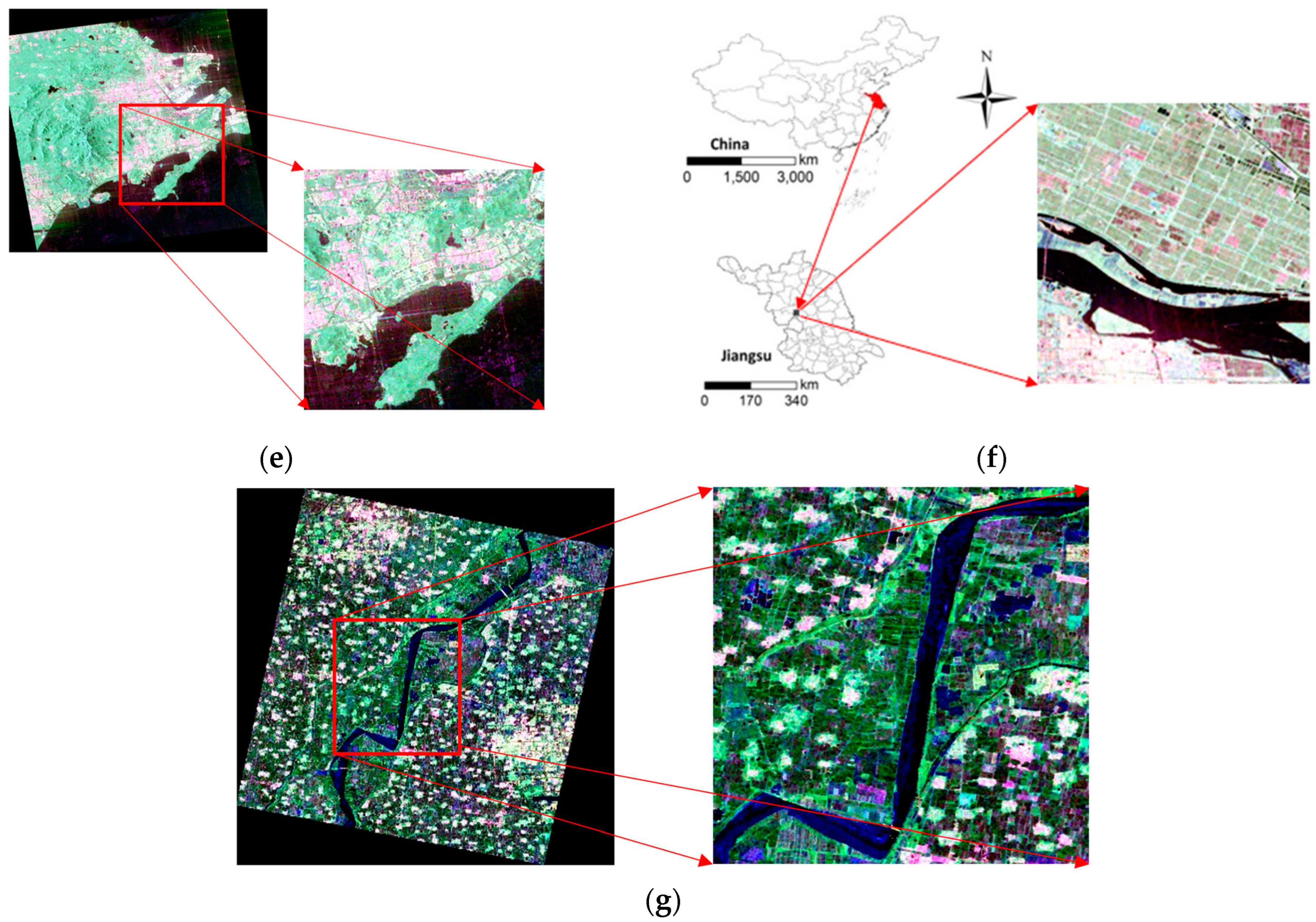
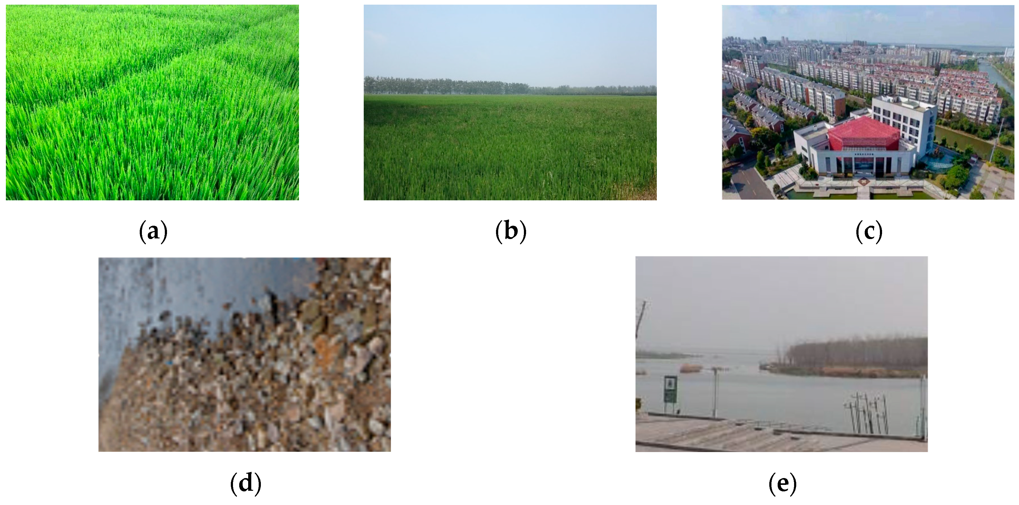
2.1. Study Area

The study area includes four regions: San Francisco, USA; Qingdao, China coastal area; rice area in Jiangsu, China; and wheat area in Yellow River, China. For San Francisco, the area is roughly divided into water, vegetation, urban, etc., and there are distinct differences among various ground objects. For Qingdao, the area includes water, vegetation, and urban. This area is a coastal area similar to San Francisco and is an ideal research area for cross-domain classification research. For rice areas in Jiangsu, the vegetation in this area is mainly rice. Due to the different selection of rice varieties and planting methods by farmland operators, this area is mainly divided into two different types of rice, namely direct-sown japonica rice paddy (D-J) and transplanting hybrid rice paddy (T-H). And other ground objects include urban, shoals, and water. For the wheat area in Yellow River, the vegetation in this area is mainly wheat, and the wheat type is winter wheat. We selected the rice planting area and the Yellow River wheat area as the study area to study the cross-domain classification of crops based on GCP SAR data. Figure 1 shows the Pauli decomposition pseudo-color image of the study area.

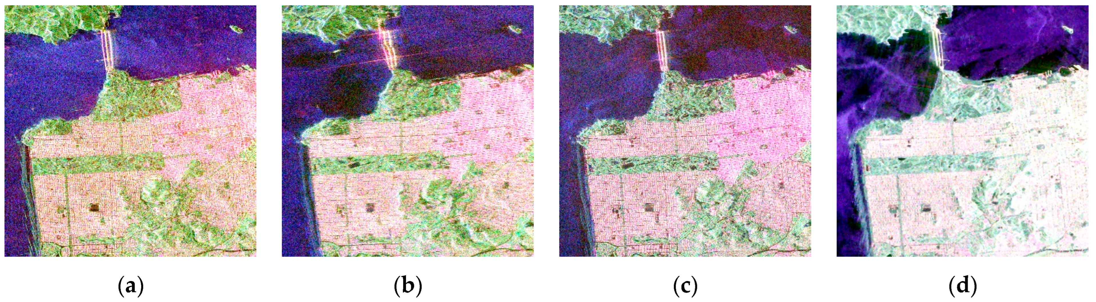
2.2. Data Collection

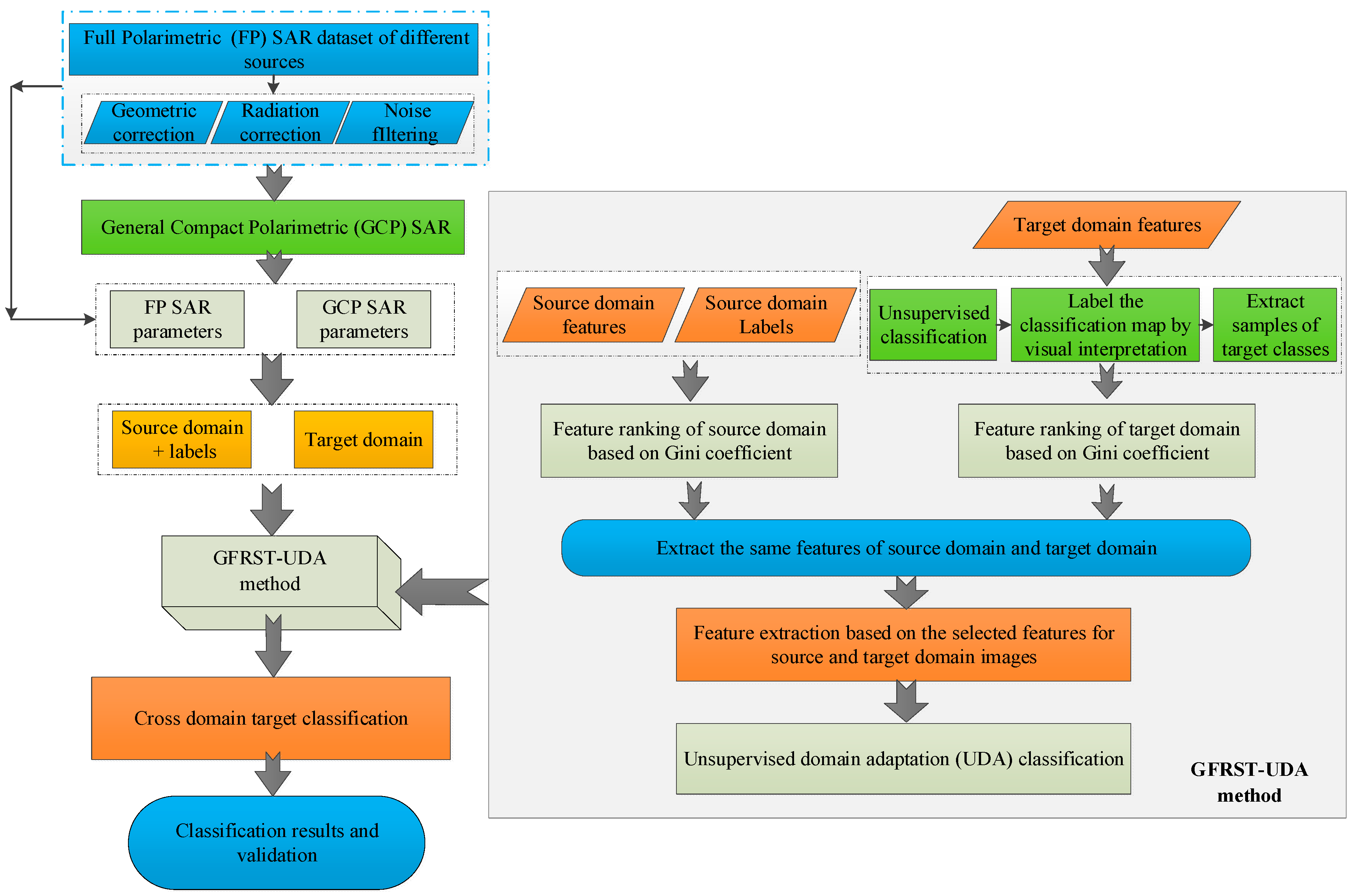
For the study area, we acquired seven SAR images from seven radar satellites, where the SAR frequency band is the C or L band. For San Francisco, we selected FP SAR data of four radar satellites, including RADARSAT-2 and GF-3 C band, ALOS-1 PALSAR-1, and ALOS-2 PALSAR-2 L band (Fine-Quad) single-look complex (SLC) data, respectively. For Qingdao, we selected GF-3 C band FP SAR data. For the rice area in Jiangsu, we selected RADARSAT-2 C band FP SAR data. The data were acquired on 16 September 2015, and the phenological period of rice is the Heading–Flowering stage. Rice paddies in this period are in the growth stage, showing typical rice characteristics on radar images. For the wheat area in Yellow River, we also selected RADARSAT-2 C band FP SAR data. The image acquisition time is 31 March 2023, and the wheat phenological period is a regreening–elongation stage, which shows typical wheat characteristics on radar images. In particular, the SAR images covering rice and wheat regions during two phenological stages are suitable for cross-domain crop classification research.

Table 1. FP SAR data parameters of multiple radar satellite data for the multi-study area.

Data Acquisition (D/M/Y)	SAR Frequency Band	Pixel Spacing (A × R, m)	Center Incidence Angle (°)	Study Area	Satellite Sensor
9 April 2008	C band	4.73 × 4.82	28.92	San Francisco, CA, USA	RADARSAT-2
11 November 2009	L band	9.37 × 3.54	23.87	San Francisco, CA, USA	ALOS-1 PALSAR-1
24 March 2015	L band	2.86 × 3.21	33.88	San Francisco, CA, USA	ALOS-2 PALSAR-2
27 March 2018	C band	2.25 × 5.79	31.35	San Francisco, CA, USA	GF-3
20 September 2017	C band	4.50 × 5.00	48.75	Qingdao, China	GF-3
16 September 2015	C band	5.20 × 7.60	39.95	Jiangsu, China	RADARSAT-2
31 March 2023	C band	4.73 × 4.74	26.70	Yellow River, China	RADARSAT-2

shows the detailed parameter information of seven FP SAR data of multiple radar satellite data for the multi-study area.

For seven FP SAR data, based on the new method proposed in this study, four types of cross-domain classification include cross-domain classification of GCP data from different sensors over the same area, GCP data acquired over different areas, FP + GCP data over different areas, and FP + GCP data over different crop types. In addition, for Jiangsu, when the RADARSAT-2 satellite transits, field surveyors use the high-precision Global Positioning System (GPS) to obtain the boundaries of these five kinds of ground objects as ground truth data, including thirty-five rice sample parcels (twenty-four T-H plots and eleven D-J plots) and eight water, eight shoal, and ten urban plots. Figure 2 shows field investigation pictures of five kinds of ground objects in Jiangsu. Furthermore, for Yellow River, when the RADARSAT-2 satellite transits, we also conduct field experiments. We use GPS to obtain the boundaries of these three kinds of ground objects as ground truth data. Figure 3 shows field investigation pictures of three kinds of ground objects in the Yellow River.

3. Methodology

For the seven FP SAR data in the study areas, first of all, data preprocessing is carried out, including radiometric calibration, geometric correction, and speckle noise filtering. In particular, the parameters required for the radiometric calibration phase are provided by the original FP SAR data header file. And we resample the image to 10 × 10 m. In addition, the image is speckle-filtered using a 7 × 7 Lee filter. Then, the unified framework of GCP is constructed, and the source domain and target domain datasets are selected to extract GCP and FP feature parameters. Furthermore, based on the proposed novel GFRST-UDA method, the source and target domains are transferred to the same feature space. Finally, the supervised classification and validation of the cross-domain target domain are carried out based on the supervision classification method. Figure 4 shows the flow chart of the methodology. In addition, a detailed description of the GFRST-UDA method in the flow chart is presented in Section 3.2.

3.1. FP/GCP SAR Feature Extraction

3.1.1. GCP SAR Data

The electromagnetic field is often represented in the form of a transverse ellipse, which contains two parameters, namely the ellipse orientation angle θ and the ellipticity angle χ, as follows [7,8]:

$${\overrightarrow{E}}_i\left(\theta ,\chi \right)=\left[\begin{array}{c}a\\ b\end{array}\right]=\left[\begin{array}{cc}\cos \theta & -\sin \theta \\ \sin \theta & \cos \theta \end{array}\right]\left[\begin{array}{c}\cos \chi \\ j\sin \chi \end{array}\right]=\left[\begin{array}{c}\cos \theta \cos \chi -j\sin \theta \sin \chi \\ \sin \theta \cos \chi +j\cos \theta \sin \chi \end{array}\right]$$

(1)

where a and b are the complex values of the transmitting wave and ${\left|a\right|}^2+{\left|b\right|}^2=1$. For an arbitrary scattering matrix S, the CP signal is totally dependent on θ and χ. For left circular, right circular, and linear $\mathsf{\pi }/4$ transmitted waves, the values of $\left(\begin{array}{cc}\theta ,& \chi \end{array}\right)$ are $\left(\left[\begin{array}{cc}-\mathsf{\pi }/2& \mathsf{\pi }/2\end{array}\right]\begin{array}{cc},& \mathsf{\pi }/4\end{array}\right)$, $\left(\begin{array}{cc}\left[\begin{array}{cc}-\mathsf{\pi }/2& \mathsf{\pi }/2\end{array}\right],& -\mathsf{\pi }/4\end{array}\right)$, and $\left(\begin{array}{cc}\mathsf{\pi }/4,& 0\end{array}\right)$. In addition, in this study, four typical GCP modes, including left circular, two elliptical polarizations, and linear $\mathsf{\pi }/4$ transmitted waves, are discussed, respectively, with the values of $\left(\begin{array}{cc}\theta ,& \chi \end{array}\right)$ as $\left(\mathsf{\pi }/4\begin{array}{cc},& \mathsf{\pi }/4\end{array}\right)$, $\left(\begin{array}{cc}\mathsf{\pi }/4,& \mathsf{\pi }/6\end{array}\right)$, $\left(\begin{array}{cc}\mathsf{\pi }/4,& \mathsf{\pi }/8\end{array}\right)$ and $\left(\begin{array}{cc}\mathsf{\pi }/4,& 0\end{array}\right)$. Then, for any transmitting wave ${\overrightarrow{E}}_i\left(\begin{array}{cc}\theta ,& \chi \end{array}\right)$, the receiving wave ${\overrightarrow{E}}_r\left(\begin{array}{cc}\theta ,& \chi \end{array}\right)$ is as follows:

$${\overrightarrow{E}}_r\left(\theta ,\chi \right)=S{\overrightarrow{E}}_i\left(\theta ,\chi \right)=\left[\begin{array}{cc}{S}_{\mathrm{HH}}& S_{\mathrm{HV}}\\ S_{\mathrm{VH}}& S_{\mathrm{VV}}\end{array}\right]\left[\begin{array}{c}a\\ b\end{array}\right]=\left[\begin{array}{c}a{S}_{\mathrm{HH}}+b{S}_{\mathrm{HV}}\\ b{S}_{\mathrm{VV}}+a{S}_{\mathrm{VH}}\end{array}\right]$$

(2)

${\overrightarrow{E}}_r\left(\begin{array}{cc}\theta ,& \chi \end{array}\right)$ in (2) is the representation of linear H/V polarization basis. Let ${\overrightarrow{E}}_r\left(\begin{array}{cc}\theta ,& \chi \end{array}\right)={\left[\begin{array}{cc}{E}_{\mathrm{H}\mathrm{C}}& E_{\mathrm{V}\mathrm{C}}\end{array}\right]}^{\mathrm{T}}$, where $E_{\mathrm{H}\mathrm{C}}=a{S}_{\mathrm{H}\mathrm{H}}+b{S}_{\mathrm{H}\mathrm{V}}$, $E_{\mathrm{V}\mathrm{C}}=b{S}_{\mathrm{V}\mathrm{V}}+a{S}_{\mathrm{V}\mathrm{H}}$, and T denotes matrix transpose. When a and b are not 0, $E_{\mathrm{H}\mathrm{C}}$ contains $S_{\mathrm{H}\mathrm{H}}$, and $E_{\mathrm{V}\mathrm{C}}$ contains $S_{\mathrm{V}\mathrm{V}}$. The backscattering characteristics of the target are mainly retained in the co-polarization ratio. When $a\ne 0$ and $b\ne 0$, the backscattering vector in (2) can be described by the formula as follows:

$$\left[\begin{array}{c}{E}_1\\ E_2\end{array}\right]=\left[\begin{array}{cc}{a}^{-1}& 0\\ 0& b^{-1}\end{array}\right]{\overrightarrow{E}}_r\left(\theta ,\chi \right)=\left[\begin{array}{c}{S}_{\mathrm{HH}}+{\displaystyle \frac{b}{a}}{S}_{\mathrm{HV}}\\ S_{\mathrm{VV}}+{\displaystyle \frac{a}{b}}{S}_{\mathrm{VH}}\end{array}\right]$$

(3)

where E₁ and E₂ are the normalized elements of ${\overrightarrow{E}}_r\left(\begin{array}{cc}\theta ,& \chi \end{array}\right)$ to represent the characteristics of backscattering waves. From (3), two new CP vectors can be expressed as:

$$\begin{array}{l}{\overrightarrow{k}}_1={\left[\begin{array}{cc}{E}_1& E_2\end{array}\right]}^{\mathrm{T}}\\ {\overrightarrow{k}}_2={\left[\begin{array}{cc}{E}_1+E_2& E_1-E_2\end{array}\right]}^{\mathrm{T}}/\sqrt{2}\end{array}$$

(4)

The corresponding second-order statistics, i.e., the compact polarization covariance matrix and coherence matrix of the normalized vector, are used to describe the partially polarized scattered wave as follows:

$$C_2=\langle {\overrightarrow{k}}_1{\overrightarrow{k}}_1^{*\mathrm{T}}\rangle =\left[\begin{array}{cc}\langle {\left|E_1\right|}^2\rangle & \langle E_1{E}_2^{*}\rangle \\ \langle E_2{E}_1^{*}\rangle & \langle {\left|E_2\right|}^2\rangle \end{array}\right]$$

(5)

$$T_2=\langle {\overrightarrow{k}}_2{\overrightarrow{k}}_2^{*T}\rangle =\left[\begin{array}{cc}\frac{\langle {\left|E_1+E_2\right|}^2\rangle }{2}& \frac{\langle \left(E_1+E_2\right){\left(E_1-E_2\right)}^{*}\rangle }{2}\\ \frac{\langle \left(E_1-E_2\right){\left(E_1+E_2\right)}^{*}\rangle }{2}& \frac{\langle {\left|E_1-E_2\right|}^2\rangle }{2}\end{array}\right]$$

(6)

where ^*T represents matrix conjugate transpose, and $〈·〉$ represents the mean value. C₂ and T₂ are obtained from two new target CP scattering vectors (k₁ and k₂) constructed based on GCP theory. It is essentially two second-order statistics of CP SAR in the same space. The GCP SAR description operator vector, covariance, and coherence matrix in (3), (5), and (6) provide a unified method for the scattering analysis of CP SAR data.

3.1.2. GCP Decomposition Parameters

The outer product of the Jones vector and its conjugate transpose vector can have a 2 × 2 Hermitian matrix:

$$E{E}^{*\mathrm{T}}=\left[\begin{array}{cc}{E}_x{E}_x^{*}& E_x{E}_{\mathrm{y}}^{*}\\ E_{\mathrm{y}}{E}_x^{*}& E_{\mathrm{y}}{E}_{\mathrm{y}}^{*}\end{array}\right]$$

(7)

Stoke vector g can be defined as [5]:

$$g=\left[\begin{array}{c}\begin{array}{c}{g}_0\\ g_1\end{array}\\ \begin{array}{c}{g}_2\\ g_3\end{array}\end{array}\right]=\left[\begin{array}{c}\begin{array}{c}{E}_x{E}_x^{*}+E_y{E}_y^{*}\\ E_x{E}_x^{*}-E_y{E}_y^{*}\end{array}\\ \begin{array}{c}{E}_x{E}_y^{*}+E_y{E}_x^{*}\\ j\left(E_x{E}_y^{*}-E_y{E}_x^{*}\right)\end{array}\end{array}\right]=\left[\begin{array}{c}\begin{array}{c}{\left|E_x\right|}^2+{\left|E_y\right|}^2\\ {\left|E_x\right|}^2-{\left|E_y\right|}^2\end{array}\\ \begin{array}{c}2\mathrm{Re}\left(E_x{E}_y^{*}\right)\\ -2\mathrm{Im}\left(E_x{E}_y^{*}\right)\end{array}\end{array}\right]$$

(8)

Based on Equations (3), (5) and (6), the Stokes vector representing the target scattering in the GCP mode is as follows:

$$g=\left[\begin{array}{c}\begin{array}{c}{g}_0\\ g_1\end{array}\\ \begin{array}{c}{g}_2\\ g_3\end{array}\end{array}\right]=\left[\begin{array}{c}\begin{array}{c}{\left|E_1\right|}^2+{\left|E_2\right|}^2\\ {\left|E_1\right|}^2-{\left|E_2\right|}^2\end{array}\\ \begin{array}{c}2\mathrm{Re}\left(E_1{E}_2^{*}\right)\\ -2\mathrm{Im}\left(E_1{E}_2^{*}\right)\end{array}\end{array}\right]$$

(9)

Based on the Stokes vector, various CP decomposition parameters in different modes can be obtained.

(1)

GCP H/α decomposition

H/α decomposition is the eigenvalue decomposition of the coherence matrix or covariance matrix of the target, and then the target is decomposed into three scattering components, and the eigenvalue and eigenvector are used to express the polarization information [41]. Some researchers have converted the H/α decomposition method in FP SAR to the H/α decomposition of CP SAR, but it can only be applied in specific CP modes [42,43]. This section extends the H/α decomposition to GCP SAR. For the GCP SAR corresponding to two polarimetric channels, the coherence matrix T₂ (Equation (6)) is a 2 × 2 nonnegative definite Hermitian matrix, and its eigenvalue decomposition is shown in Equation (10). In addition, Equation (11) is the corresponding unitary transformation matrix and the eigenvector.

$${\mathrm{T}}_2=\left[\begin{array}{cc}{\mathrm{T}}_{11}& {\mathrm{T}}_{12}\\ {\mathrm{T}}_{12}^{*}& {\mathrm{T}}_{22}\end{array}\right]=U\left[\begin{array}{cc}{\lambda }_1& \\ & {\lambda }_1\end{array}\right]U^{\mathrm{T}}={\lambda }_1{\overrightarrow{u}}_1{\overrightarrow{u}}_1^{*\mathrm{T}}+{\lambda }_2{\overrightarrow{u}}_2{\overrightarrow{u}}_2^{*\mathrm{T}}$$

(10)

where

$$\begin{array}{l}U=\left[\begin{array}{cc}{u}_{11}& u_{12}\\ u_{21}& u_{22}\end{array}\right]=\left[\begin{array}{cc}{\overrightarrow{u}}_1& {\overrightarrow{u}}_2\end{array}\right]\\ {\overrightarrow{u}}_i=e^{j{\phi }_i}{\left[\begin{array}{cc}\cos {\alpha }_i& \sin {\alpha }_i{e}^{j{\phi }_i{\delta }_i}\end{array}\right]}^{\mathrm{T}}, i=1,2\end{array}$$

(11)

After eigen decomposition of the GCP coherence matrix T₂, the polarization entropy H_CP, the average scattering angle α_CP, and the anisotropic A_CP are shown in Equations (12), (13) and (15).

$$H_{\mathrm{CP}}={\displaystyle \sum _{i=1}^2-P_i{\log }_2{P}_i}$$

(12)

$${\alpha }_{\mathrm{CP}}={\displaystyle \sum _{i=1}^2{P}_i\mathrm{arc}{\cos }^{-1}\left(\left|u_{1i}\right|\right)}$$

(13)

$$P_i=\frac{{\lambda }_i}{{\lambda }_1+{\lambda }_2}，i=1,2$$

(14)

$$A_{\mathrm{CP}}={\displaystyle \frac{{\lambda }_1-{\lambda }_2}{{\lambda }_1+{\lambda }_2}}={\displaystyle \frac{P_1-P_2}{P_1+P_2}}$$

(15)

where λ is the eigenvalue of GCP coherence matrix T₂, and the average scattering angle α_CP is from the unitary eigenvector μ_i.

(2)

GCP m-χ and m-δ decomposition

The three scattering components of the m-χ and m-δ decomposition, the physical meanings of which are similar to those of the Freeman–Durden decomposition [44] for FP SAR, are generated from the GCP SAR data as described by Equations (16)–(20) [10,11].

$$m=\sqrt{\left(g_1^2+g_2^2+g_3^2\right)}/g_0$$

(16)

$$\sin 2\chi =-g_3/\left(m{g}_0\right)$$

(17)

$$\delta =\arg (g_2+j{g}_3)$$

(18)

where m is the degree of polarization, δ is the relative phase, and χ is the ellipticity angle of the Poincaré sphere. They are all the child parameters of the Stokes vector, which can be obtained based on the Stokes vector of GCP systems from Equation (9). The Stokes parameter g₀, which is the total backscattered energy received by GCP systems, in combination with the GCP parameters m, δ, and χ, was used to generate the m-δ (as shown in Equation (19)) and m-χ decompositions (as shown in Equation (20)), respectively. P_d, P_v, and P_s correspond to double-bounce, the randomly polarized constituent (volume), and surface scattering.

$${\left[\begin{array}{c}{P}_d\\ P_v\\ p_s\end{array}\right]}_{m-\delta }=\left[\begin{array}{c}\sqrt{m{g}_0\left(1+\sin \delta \right)/2}\\ \sqrt{g_0\left(1-m\right)}\\ \sqrt{m{g}_0\left(1-\sin \delta \right)/2}\end{array}\right]$$

(19)

$${\left[\begin{array}{c}{P}_d\\ P_v\\ p_s\end{array}\right]}_{m-\chi }=\left[\begin{array}{c}\sqrt{m{g}_0\left(1-\sin 2\chi \right)/2}\\ \sqrt{g_0\left(1-m\right)}\\ \sqrt{m{g}_0\left(1+\sin 2\chi \right)/2}\end{array}\right]$$

(20)

(3)

GCP m-α_s decomposition

The m-α_s decomposition method is similar to the m-δ method. The symmetric scattering type α_s is closely related to the ellipticity of the compact scattered wave. α_s is in the [0, $\mathsf{\pi }/2$]. Here, 0 represents surface scattering, and $\mathsf{\pi }/2$ represents double-bounce scattering. From the first Stokes component (g₀), the symmetric scattering type (α_s) and the degree of polarization (m) were used to generate the m-α_s feature decomposition basis [12,45]:

$${\alpha }_{\mathrm{s}}={\displaystyle \frac{1}{2}}{\tan }^{-1}\left({\displaystyle \frac{\sqrt{g_1^2+g_2^2}}{\pm g_3}}\right)$$

(21)

$${\left[\begin{array}{c}{P}_d\\ P_v\\ p_s\end{array}\right]}_{m-{\alpha }_{\mathrm{s}}}=\left[\begin{array}{c}m{g}_0\left(1-\cos 2{\alpha }_{\mathrm{s}}\right)/2\\ g_0\left(1-m\right)\\ m{g}_0\left(1+\cos 2{\alpha }_{\mathrm{s}}\right)/2\end{array}\right]$$

(22)

Finally, based on the aforementioned GCP SAR theory, we have extended the polarimetric decomposition method, originally designed for specific CP modes, to encompass the GCP mode as well. The 22 GCP feature parameter sets constructed in this study are shown in

Table 2. Feature parameters of GCP SAR data.

Parameter Extraction Method	Feature Component	Feature Number
Stokes matrix	g0, g1, g2, g3	4
Backscattering intensity	σCV, σCR, σCH, σCL [14]	4
m-δ decomposition	Ps_m-δ, Pd_m-δ, Pv_m-δ	3
m-χ decomposition	Ps_m-χ, Pd_m-χ, Pv_m-χ	3
m-αs decomposition	Ps_m-αs, Pd_m-αs, Pv_m-αs	3
H/α decomposition	H, α, A	3
ΔαBCP/αBCP decomposition	ΔαBCP, αBCP [8]	2
Total	-	22

, including Stokes parameters, child parameters of the Stokes vector, and the GCP decomposition parameters.

3.1.3. FP SAR Feature Parameters

For FP SAR, we selected 22 FP SAR parameters. The 22 FP SAR parameters include the three components of the coherence matrix and five polarimetric decomposition parameters. In addition, we introduce the rotational domain polarimetric features. Finally, the 22 FP feature parameter sets we constructed are shown in

Table 3. Feature parameters of FP SAR data.

Parameter Extraction Method	Feature Component	Feature Number
H/α decomposition	H_Full, α_Full, A_Full	3
Freeman decomposition	Ps_F, Pd_F, Pv_F	3
ΔαB/αB decomposition [46]	αB, ΔαB, Φ	3
Yamaguchi decomposition [47]	Ps_Y, Pd_Y, Pv_Y, Ph_Y	4
Pauli decomposition	Pauli_1, Pauli_2, Pauli_3	3
Polarization characteristics of the rotating domain [48]	Re[T12(θnull)], Im[T12(θnull)], Re[T23(θnull)]	3
Polarimetric coherency matrix	T11, T22, T33	3
Total	-	22

.

3.2. GFRST-UDA Method

The Gini coefficient is an indicator used to describe the degree of confusion in the system and is less computationally intensive. It represents the probability that a randomly selected sample in the sample set is misclassified. The smaller the Gini coefficient, the smaller the probability that the selected sample in the set is misclassified; that is, the higher the purity of the set; otherwise, the lower the purity of the set. Therefore, when all the samples in the set are in the same category, the Gini coefficient is 0. Based on the idea of describing the set purity of the Gini coefficient and the physical structure of trees in random forests [49], we calculate the contribution of the Gini coefficient of each feature in each tree in random forest so as to evaluate the importance of the compact polarimetric feature.

Suppose that the feature set in the source domain or target domain data is $X=\left\{x_1,x_2,\cdots ,x_J\right\}$, J represents the number of features, and the number of classes is c. There are I decision trees in the random forest, then the Gini coefficient of the node q in the decision tree i is:

$$G_q^i={\displaystyle \sum _{c=1}^C{\displaystyle \sum _{c^{\prime }\ne c}{p}_q^i\left(c\right)p_q^i\left(c^{\prime }\right)=1-}}{\displaystyle \sum _{c=1}^C{\left(p_q^i\left(c\right)\right)}^2}$$

(23)

where $p_q\left(c\right)$ denotes the proportion of class c in node q. $p_q\left(c^{\prime }\right)$ denotes the proportion that is not class c in node q. For feature j, the change in its Gini coefficient on node q can be obtained by calculating the difference between the Gini coefficient of the feature before and after branching of the node. The change in the Gini coefficient here is the importance of feature j in node q of decision tree i, and the formula is:

$$V_q^i\left(j\right)=G_q^i-G_r^i-G_s^i$$

(24)

where $G_r^i$ and $G_s^i$ represent the Gini coefficient of the two new nodes after the node q of the decision tree i is branched, respectively. From this, the importance of feature x_j in decision tree i can be obtained:

$$M_j^i={\displaystyle \sum _{q\in Q}{V}_q^i\left(j\right)}$$

(25)

where Q denotes the set of nodes that feature x_j appears in decision tree i. When the contribution of feature x_j on each tree is obtained, the total contribution of x_j in the random forest can be obtained:

$$M_j={\displaystyle \sum _{i=1}^I{M}_j^i}$$

(26)

To facilitate the comparison of the contribution between each feature, the values are normalized:

$$VI{M}_j={\displaystyle \frac{M_j}{{\displaystyle \sum _{k=1}^J{M}_k}}}$$

(27)

By comparing the normalized contribution of each feature VIM_j, the priority ranking of each feature can be obtained. In summary, in a random forest, the Gini coefficient is used to select the best feature when the decision tree nodes are split. By comparing the change in the Gini coefficient when splitting with different features, the contribution of each feature to the purity improvement of the model can be assessed. The smaller the Gini coefficient, the greater the contribution of the feature to the purity of the model and the greater its importance. Therefore, in the GFRST-UDA proposed in this study, we introduce the Gini coefficient to rank the SAR feature parameters so as to select the feature parameters that contribute greatly to the classification effect.

The essential principle of the UDA method is to convert the features of the source domain and target domain, which are not similar in different spaces, into the same feature space. The degree of feature alignment may be affected when the feature is insufficient or excessive. Therefore, this study considers taking the lead in ranking and optimizing the features of both the source and target domains and then introducing different UDA methods for feature transfer. Since there are class labels in the source domain, the features of the source domain can be directly sorted and optimized based on the Gini coefficient. However, its optimal feature parameters are not necessarily effective for the classification effect of the target domain. Therefore, we consider feature selection based on the Gini coefficient for both source domain and target domain features, that is, select the parameters that contribute greatly to the classification of the source domain and target domain and then perform feature transfer based on different UDA methods.

However, since there are no class labels in the target domain, it is impossible to sort and optimize the target domain features directly. Therefore, we consider the unsupervised classification of the target image, and then the classification results are visually interpreted to give a small number of pseudo-labels of the determined ground-object classes. Finally, polarimetric features are sorted and optimized based on the target domain with pseudo-labels. The specific GFRST-UDA method can be divided into four steps.

Step 1: Firstly, a random forest model is constructed on labeled source domain data, and then the Gini coefficient of each node in each decision tree in the source domain is calculated. The contribution VIM of each feature is obtained by Equations (24)–(27). Then, all the source domain features are ranked in order of contribution VIM, and then the features with the top 95% contribution VIM are selected to construct the feature subset of the source domain. Among them, 95% are empirical selection, and the features that contribute little to the classification effect of the source domain are eliminated; that is, most of the contributing features are retained to avoid feature redundancy.

Step 2: The features of the target domain are first classified based on the unsupervised classification method, and then the classification map is visually interpreted, and a few pseudo-labels are given. Next, a random forest model of the target domain is constructed on the target domain with pseudo-label data. Moreover, as in step 1, all the target domain features are ranked in order of contribution VIM, and then the features with the top 95% contribution VIM are selected to construct the feature subset of the target domain.

Step 3: If the optimal feature parameters have contributed to the feature classification effect of both the source and target domains, the feature alignment effect of the optimal feature parameters will also be improved after the source and target domains are converted into the same space. Therefore, this step is to obtain the intersection of the optimal feature subset of the source domain and the optimal feature subset of the target domain to obtain the GFRST feature subset, which has a high contribution to the classification effect of the source domain and the target domain.

Step 4: Based on the GFRST feature subset, varieties of UDA methods are introduced for feature alignment, and the source and target domains are converted to the same feature space. Finally, the target domain after feature alignment is classified based on the supervised classification method to achieve cross-domain image classification. When evaluating the feature alignment effect of source and target domains, we introduce the concept of discrete coefficients to calculate the intra-class and inter-class discrete coefficients of source and target domains before and after alignment. The dispersion coefficient represents the dispersion degree of overall unit values, and the smaller the value, the smaller the dispersion degree. When the difference between the dispersion coefficients of the source and target domains after feature alignment is small, it is considered that the feature alignment effect is satisfactory. Otherwise, the feature alignment effect is poor. Discrete coefficients C_v can be defined as:

$$C_v={\displaystyle \frac{\sigma }{\mu }}$$

(28)

$$\sigma =\sqrt{{\displaystyle \frac{{\displaystyle \sum {(X-\mu )}^2}}{N}}}$$

(29)

$$\mu =\sqrt{{\displaystyle \frac{{\displaystyle \sum _{i=1}^{N}Xi}}{N}}}$$

(30)

where σ represents the standard deviation of the source or target domain, μ is the sample mean of the source or target domain, and N indicates the number of samples from the source domain or target domain.

In addition, in this study, we use seven UDA methods, including Subspace Alignment (SA) [50], Transfer Component Analysis (TCA) [30], Joint Distribution Adaptation (JDA), CORrelation Alignment (CORAL), Balanced Distribution Adaptation (BDA), Geodesic Flow Kernel (GFK), and Manifold Embedded Distribution Alignment (MEDA) methods, respectively [51,52,53,54,55]. In the feature alignment of domain adaptation, the construction of a domain adaptation optimization target is the key. For the SA method, the source domain is represented by the source subspace SX_S and the target domain is represented by the target subspace TX_T. S and T are the original data features of the source domain and the target domain, respectively. X_S and X_T are the eigenmatrices composed of the front D-dimensional eigenvectors after the transformation of the source domain and the target domain through principal component analysis, respectively. It is worth noting that in the experiment, D of D-dimensional eigenvectors is the number of optimal feature subsets based on the GFRST method. Furthermore, the linear transformation function M is obtained by minimizing the divergence of the Bregman matrix from X_S to X_T.

$$F(M)={\Vert X_{S}M-X_T\Vert }_F^2$$

(31)

$$M^{*}=\underset{M}{argmin(F(M))}=X_s^T{X}_T$$

(32)

where ${\Vert \cdot \Vert }_F^2$ indicates the Frobenius norm. The subspace after source domain alignment is SX_SM^*, and the subspace after target domain alignment is TX_T.

SA only performs first-order feature alignment between the source domain and the target domain, while CORAL performs second-order feature alignment between the two domains. In this study, C_S and C_T are defined as covariance matrices of source and target domains, respectively, and covariance alignment is to learn a second-order feature transformation A to minimize the feature distance between the source domain and the target domain. Its optimization objective function is as follows:

$$\underset{A}{\min }{\Vert C_S-C_T\Vert }_F^2=\underset{A}{\min }{\Vert A^T{C}_{S}A-C_T\Vert }_F^2$$

(33)

$$z^r=\{\begin{array}{c}{x}^r\cdot {(C_S+E_S)}^{-\frac{1}{2}}\cdot {(C_T+E_T)}^{-\frac{1}{2}},r=s\\ x^r,r=t\end{array}$$

(34)

where E_S and E_T are identity matrices with the same size of source and target domains, respectively.

In addition, TCA, JDA, BDA, and MEDA methods are used to construct optimization objective functions by calculating the maximum mean difference in the edge distribution, the maximum mean difference in the conditional distribution, and the maximum mean difference based on adaptive factors, respectively. Following the alignment of features through domain adaptation, supervised classification is subsequently performed using a typical supervised classifier. In this study, the supervised classifier we select is the K-Nearest Neighbor classifier.

4. Results and Discussion

Based on the methodology in Section 2, the cross-domain classification is carried out from four aspects, which include cross-domain classification of GCP data from different sensors over the same area, GCP data acquired over different areas, FP + GCP data over different areas, and FP + GCP data over different crop types. For the four aspects, we label the cross-domain classification groups as experimental transfer groups 1, 2, 3, and 4.

Table 4. Experimental groups for different cross-domain classification.

Experimental Transfer Group 1		Experimental Transfer Group 2		Experimental Transfer Group 3		Experimental Transfer Group 4
	Source Domain→Target Domain		Source Domain→Target Domain		Source Domain→Target Domain		Source Domain→Target Domain
a	ALOS1-Sanf→RS2-Sanf	a	GF3-Qingdao→RS2-Sanf	a	GF3-Qingdao→RS2-Sanf	a	GF3-Qingdao→RS-2 Yellow River
b	ALOS2-Sanf→RS2-Sanf	b	GF3-Qingdao→ALOS1-Sanf	b	GF3-Qingdao→ALOS1-Sanf	b	RS2-Qingdao→RS-2 Yellow River
c	GF3-Sanf→RS2-Sanf	c	GF3-Qingdao→ALOS2-Sanf	c	GF3-Qingdao→ALOS2-Sanf	c	Jiangsu T-H→RS-2 Yellow River
d	RS2-Sanf→ALOS1-Sanf	d	GF3-Qingdao→GF3-Sanf	d	GF3-Qingdao→GF3-Sanf	d	Jiangsu D-J→RS-2 Yellow River
e	ALOS2-Sanf→ALOS1-Sanf	e	ALOS2-Sanf→GF3-Qingdao	e	RS2-Sanf→GF3-Qingdao	-
f	GF3-Sanf→ALOS1-Sanf	-		f	ALOS1-Sanf→GF3-Qingdao	-
g	RS2-Sanf→ALOS2-Sanf	-		g	ALOS2-Sanf→GF3-Qingdao	-
h	ALOS1-Sanf→ALOS2-Sanf	-		h	GF3-Sanf→GF3-Qingdao	-
i	GF3-Sanf→ALOS2-Sanf	-		-		-
j	RS2-Sanf→GF3-Sanf	-		-		-
k	ALOS1-Sanf→GF3-Sanf	-		-		-
l	ALOS2-Sanf→GF3-Sanf	-		-		-

shows the experimental groups for different cross-domain classifications.

4.1. Cross-Domain Image Classification Based on the GCP SAR Images

4.1.1. Images from Different Sensors over the Same Area

As shown in Table 4, the experimental transfer group 1 includes 12 cross-domain image pairs involving four FP SAR data from different radar satellites in San Francisco. Based on GCP theory, 22 CP parameters are extracted from four FP SAR data, and then cross-domain classification is studied based on the GFRST-UDA method.

(1)

GFRST feature selection

Taking the CP SAR data with circular polarization transmitting as an example, based on the GFRST method feature selection, the optimal feature subset that contributes to feature alignment is selected. Figure 5 shows the feature importance ranking for CP SAR data with circular polarization transmitting. There are obvious differences in feature importance ranking for the four CP SARs. The reason is that although the data are acquired in the same area, due to the different radar imaging frequency bands and imaging time, the differences in various scattering characteristics are obvious, so the ranking results are different. It can be seen from

Table 5. Feature selection parameters based on the GFRST method for CP SAR data with circular polarization transmitting.

	RS2→ALOS1	RS2→ALOS2	RS2→GF3	ALOS1→ALOS2	ALOS1→GF3	ALOS2→GF3
Feature Number	13	11	13	13	11	11
Optimal parameters	Pd_m-δ, g1, σCL, Pd_m-χ, Pd_m-αs, g0, αBCP, σCR, α, σCH, Pv_m-αs, Pv_m-δ, Pv_m-χ	Pd_m-δ, g1, σCL, Pd_m-χ, Pd_m-αs, g0, σCR, σCH, Pv_m-αs, Pv_m-δ, Pv_m-χ	g1, σCL, Pd_m-αs, g0, αBCP, σCR, α, σCH, Pv_m-αs, Pv_m-δ, Pv_m-χ, H, A	Ps_m-αs, Pd_m-αs, Pd_m-χ, Pd_m-δ, g1, σCV, σCL, σCR, g0, Pv_m-δ, σCH, Pv_m-χ, Pv_m-αs	αBCP, α, Pd_m-αs, g1, σCL, σCR, g0, Pv_m-δ, σCH, Pv_m-χ, Pv_m-αs	Ps_m-δ, g1, Ps_m-χ, Pd_m-αs, Pv_m-αs. Pv_m-δ σCR. Pv_m-χ, σCL, g0, σCH

that 22 CP parameters retain about half of the CP parameters after feature selection based on the GFRST method. The CP decomposition parameters, including the double-bounce scattering component (Pd_m-α_s) and the volume scattering component (Pv_m-δ and Pv_m-χ), are selected for the optimal feature set in the six cross-domain image pairs. The main reason is that the decomposition parameters are significantly different in the source and target domains’ three types of ground objects. Two backscattering coefficients (σ_CR, σ_CH) and Stokes component g₀ that represent the total power of the planar electromagnetic wave are also selected to the optimal feature set for each of the six cross-domain image pairs. These optimal features can describe the target stably under different scenes.

(2)

Evaluation of cross-domain classification results based on the GFRST-UDA method

After feature selection based on the GFRST-UDA method, we use seven UDA methods to classify the target domains of 12 cross-domain image pairs, respectively. It can be seen from

Table 6. The overall accuracy of cross-different sensors classification based on the GFRST-UDA method for CP SAR data with circular polarization transmitting.

	ALOS1→RS2	ALOS2→RS2	GF3→RS2	RS2→ALOS1	ALOS2→ALOS1	GF3→ALOS1	RS2→ALOS2	ALOS1→ALOS2	GF3→ALOS2	RS2→GF3	ALOS1→GF3	ALOS2→GF3
GFRST-SA	0.938	0.961	0.935	0.832	0.958	0.821	0.895	0.948	0.726	0.945	0.914	0.804
GFRST-TCA	0.936	0.968	0.935	0.842	0.940	0.882	0.879	0.905	0.863	0.945	0.931	0.779
GFRST-JDA	0.943	0.963	0.949	0.847	0.947	0.835	0.953	0.951	0.926	0.940	0.917	0.940
GFRST-CORAL	0.922	0.956	0.934	0.793	0.957	0.807	0.797	0.959	0.795	0.950	0.921	0.782
GFRST-BDA	0.943	0.965	0.949	0.847	0.947	0.836	0.839	0.951	0.926	0.940	0.917	0.940
GFRST-GFK	0.940	0.956	0.940	0.831	0.959	0.822	0.894	0.949	0.728	0.942	0.914	0.803
GFRST-MEDA	0.944	0.968	0.970	0.841	0.946	0.930	0.967	0.942	0.960	0.937	0.921	0.939
Supervised classification	0.987			0.977			0.944			0.979

that the GFRST-UDA method has the ability to achieve high cross-different sensors classification accuracy, and the overall accuracy can reach more than 80%. For various GFRST-UDA methods, the cross-domain classification results of each pair exhibit slight variations. Moreover, even under the same GFRST-UDA method, there are subtle differences in the classification results of cross-domain images from radar satellites. This is attributed to the varying performance of different methods and dissimilarities in the distribution of features between source and target domains.

It is evident from Figure 6 that the cross-domain classification accuracy between C-band radar satellite SAR data as the source domain and L-band radar satellite SAR data as the target domain achieves an overall accuracy of approximately 78%. However, when L-band radar satellite SAR data serve as the source domain and C-band radar satellite SAR data act as the target domain, the cross-domain classification accuracy surpasses 85%. The reasons primarily lie in two aspects. Firstly, in cross-domain classification, not all CP parameters contribute positively to the classification of ground objects, and feature redundancy exists. Secondly, multi-source CP SAR parameters exhibit diverse representations of scattering information for various ground objects in the cross-domain classification of multi-source SAR. The second reason lies in the inherent difficulty of improving cross-domain classification due to the heterogeneity of radar satellite sensors across different frequency bands. However, the GFRST-UDA method effectively extracts CP SAR parameters contributing to classification results in both source and target domains, thereby mitigating cross-domain imbalance to some extent (Figure 7a). Additionally, Figure 7b presents the classification accuracy of four methods for 12 cross-domain image pairs. The GFRST-UDA method exhibits higher classification accuracy than both the UDA and GFRS (Gini coefficient feature ranking only in the source domain)-UDA methods, with results closest to those obtained through supervised classification.

Using the ALOS1-Sanf→GF3-Sanf cross-domain pair as an example, Figure 8 displays cross-domain images (ALOS1-Sanf→GF3-Sanf) classification maps for CP SAR data. Comparing the results of Figure 8a–d, it can be observed that the GFRST-SA result (Figure 8c) significantly outperforms Figure 8a,b. Particularly in the black frame area where the ground truth is pure water, misclassification occurs in Figure 8a,b, while Figure 8c produces accurate classification results. The resulting map from Figure 8c is also closest to the supervised classification result map (Figure 8d).

To validate the efficacy of GFRST-UDA in feature alignment, Figure 9 illustrates the scatter plots of source and target domains’ feature alignment. It is evident from Figure 9 that the source and target domains do not share the same feature space. By applying the JDA method, we can align the features of both domains to a common space, denoted as Figure 9b,b₁,b₂ for the aligned source domain and Figure 9c,c₁,c₂ for the aligned target domain. From Figure 9b,c, it is evident that the feature alignment between source and target domains is highly effective after the process. Specifically, compared to Figure 9b,c, and Figure 9b₁,c₁ alignments, Figure 9b₂,c₂ alignments exhibit better results for water classes. Therefore, GFRST-JDA methods outperform JDA and GFRS-JDA approaches in terms of feature alignment. To quantitatively measure the impact of the GFRST-UDA on feature alignment, we computed the inter-class and intra-class dispersion coefficients for both source and target domains before and after feature alignment. The dispersion coefficient indicates the degree of discreteness in overall unit values, with smaller values indicating less dispersion. Figure 10 shows the histograms of the dispersion coefficient of source and target domains and aligned source and target domains. Compared to Figure 10a,b, the inter-class and intra-class dispersion coefficients of both source and target domains after alignment in Figure 10c are the most similar. Conversely, Figure 10a,b exhibit significant differences in these same coefficients between the two domains. Therefore, quantitative analysis of discrete coefficients can further verify GFRST-UDA’s efficacy in feature alignment.

4.1.2. Images Acquired over Different Areas

As shown in Table 4, the experimental transfer group 2 includes five cross-domain image pairs involving five FP SAR data from different radar satellites in San Francisco and Qingdao.

Table 7. The overall accuracy of cross-different areas classification based on the GFRST-UDA method for CP SAR data with circular polarization transmitting.

	GF3-Qingdao→RS2-Sanf	GF3-Qingdao→ALOS1-Sanf	GF3-Qingdao→ALOS2-Sanf	GF3-Qingdao→GF3-Sanf	ALOS2-Sanf→GF3-Qingdao
GFRST-SA	0.913	0.957	0.884	0.899	0.908
GFRST-TCA	0.881	0.942	0.872	0.851	0.920
GFRST-JDA	0.937	0.920	0.914	0.898	0.935
GFRST-CORAL	0.839	0.948	0.896	0.891	0.524
GFRST-BDA	0.930	0.934	0.900	0.901	0.913
GFRST-GFK	0.878	0.922	0.879	0.889	0.867
GFRST-MEDA	0.901	0.915	0.869	0.874	0.914
Supervised classification	0.987	0.977	0.944	0.979	0.980

shows the overall accuracy of cross-different areas classification based on the GFRST-UDA method for CP SAR data. For various GFRST-UDA methods, the results of cross-domain classification may differ slightly but can achieve higher accuracy, with an overall accuracy exceeding 85%. The areas of Qingdao and San Francisco are both coastal areas, and the types of ground objects are similar, which is an important reason for the high accuracy of cross-domain classification. As shown in Figure 11, the cross-domain classification results based on the GFRST-UDA method outperform those based on the UDA and GFRS-UDA methods in all five cross-domain image pairs, approaching the accuracy of supervised classification results. Specifically, the GFRST-UDA method yields cross-domain classification results with an accuracy that is 3% to 5% higher than that of the UDA method.

Taking two cross-domain image pairs (GF3-Qingdao→RS2-Sanf and ALOS2-Sanf→GF3-Qingdao) as examples, Figure 12 displays cross-domain image classification results for CP SAR data. Comparing the results of Figure 12a–d, it can be observed that the GFRST-SA result (Figure 12c) significantly outperforms Figure 12a,b. Particularly in the black frame area where the ground truth is water class, misclassification occurs in Figure 12,b, while Figure 12c produces accurate classification results. The resulting map from Figure 12c is also closest to the supervised classification result map (Figure 12d). Comparing the results of Figure 12a₁–d₁, it can be observed that the GFRST-SA result (Figure 12c₁) outperforms Figure 12a₁,b₁ significantly. Particularly in the yellow frame area where the ground truth is water class, there is a phenomenon that Figure 12a₁,b₁ are misclassified as vegetation class while Figure 12c produces accurate classification results. The resulting map from Figure 12c₁ is also closest to the supervised classification result map (Figure 12d₁). Therefore, the GFRST-UDA method demonstrates superior performance in cross-domain classification of GCP data acquired over different areas, resulting in higher accuracy for cross-domain classification.

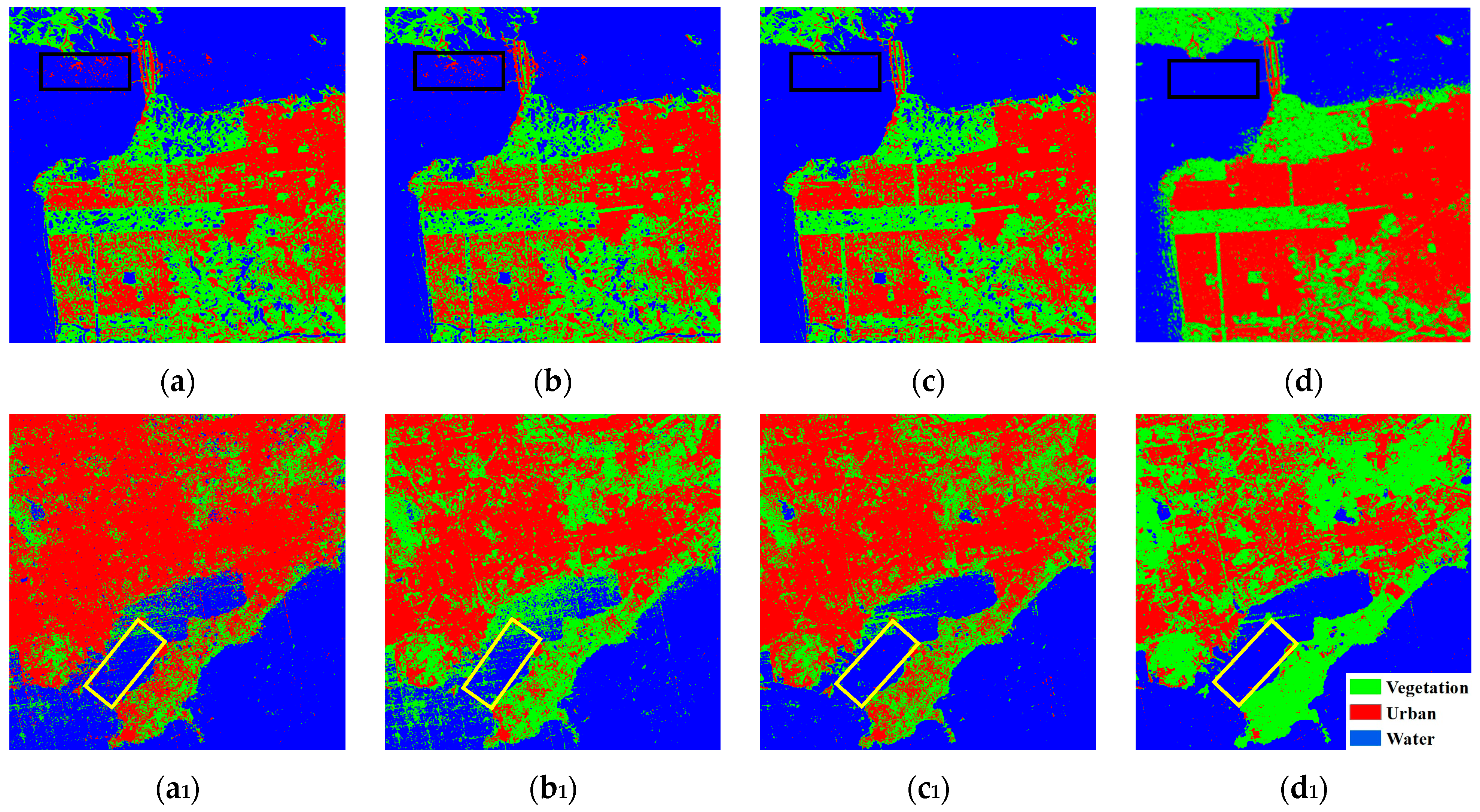
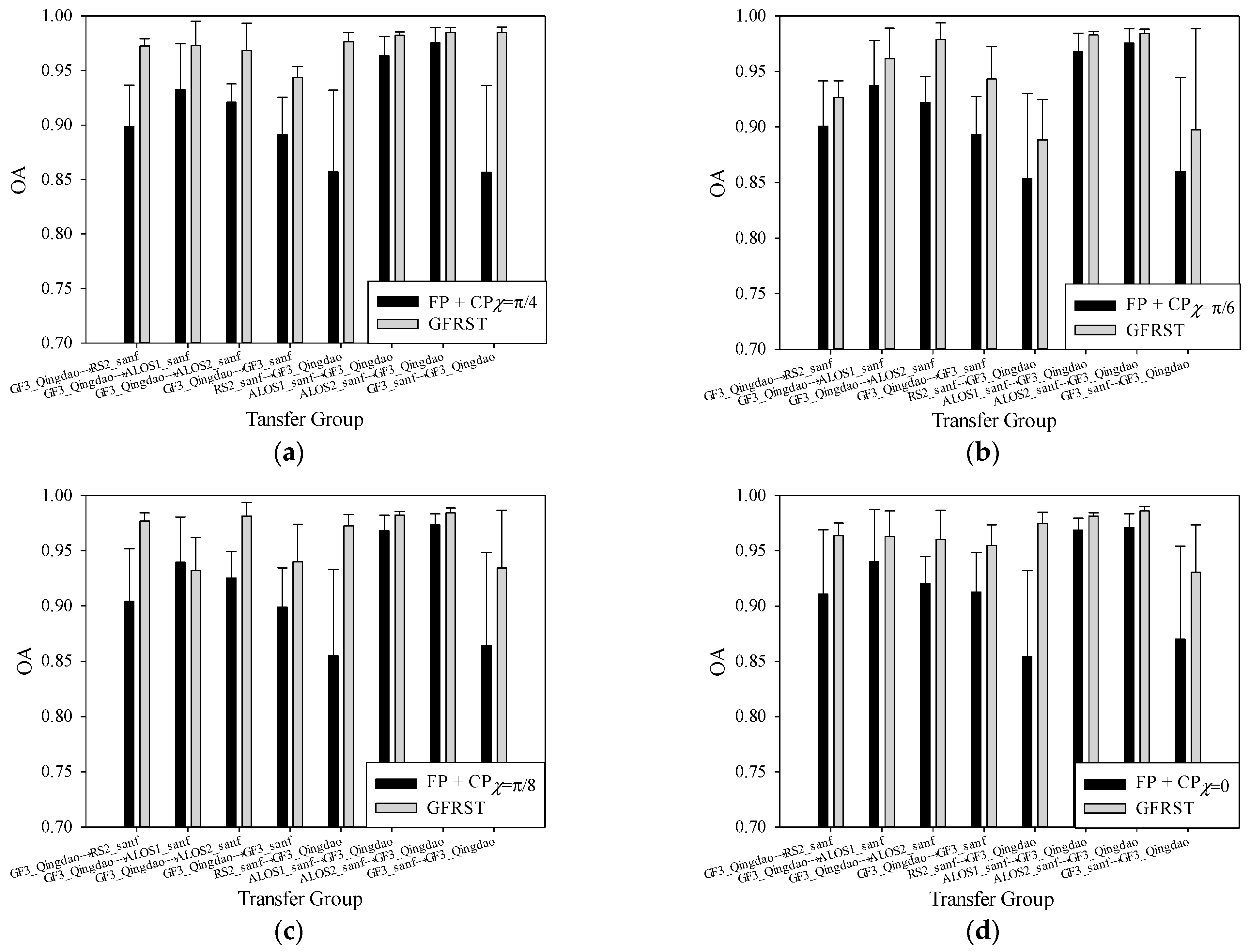
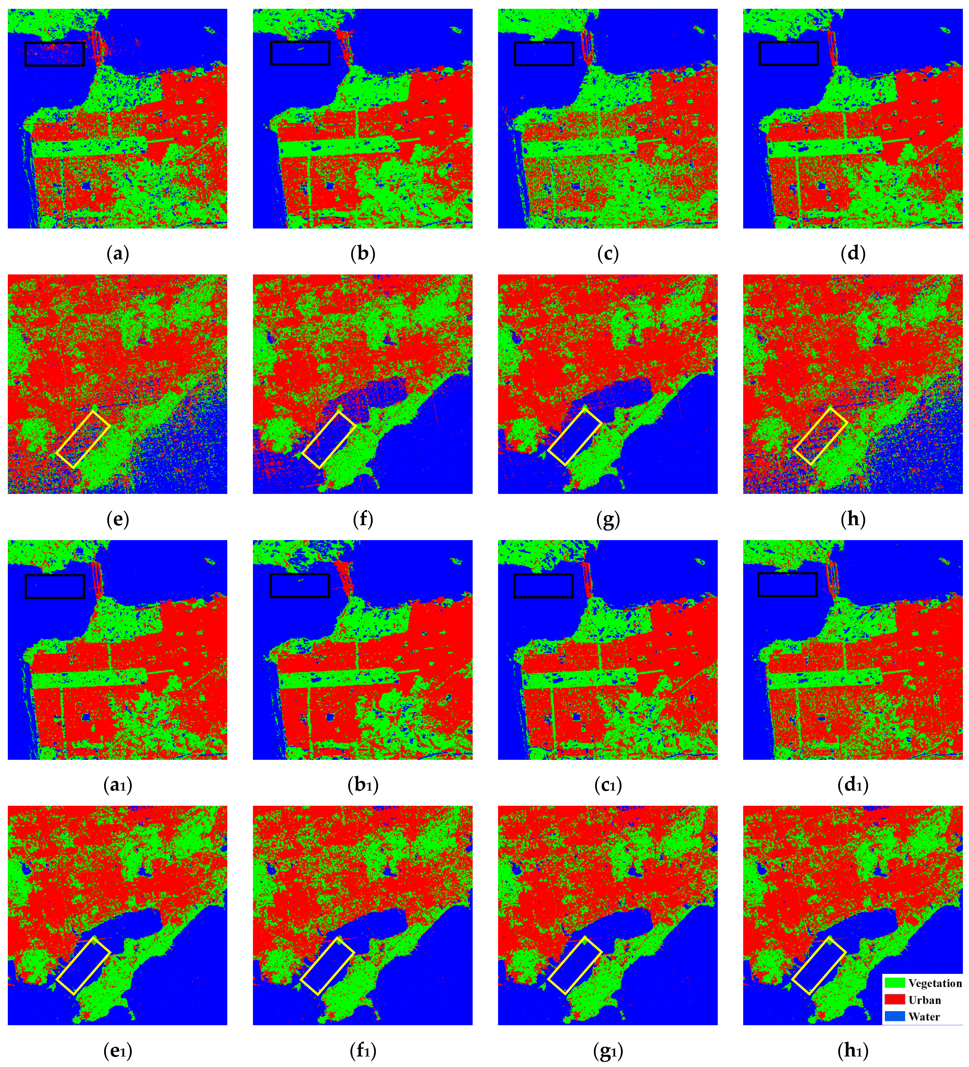
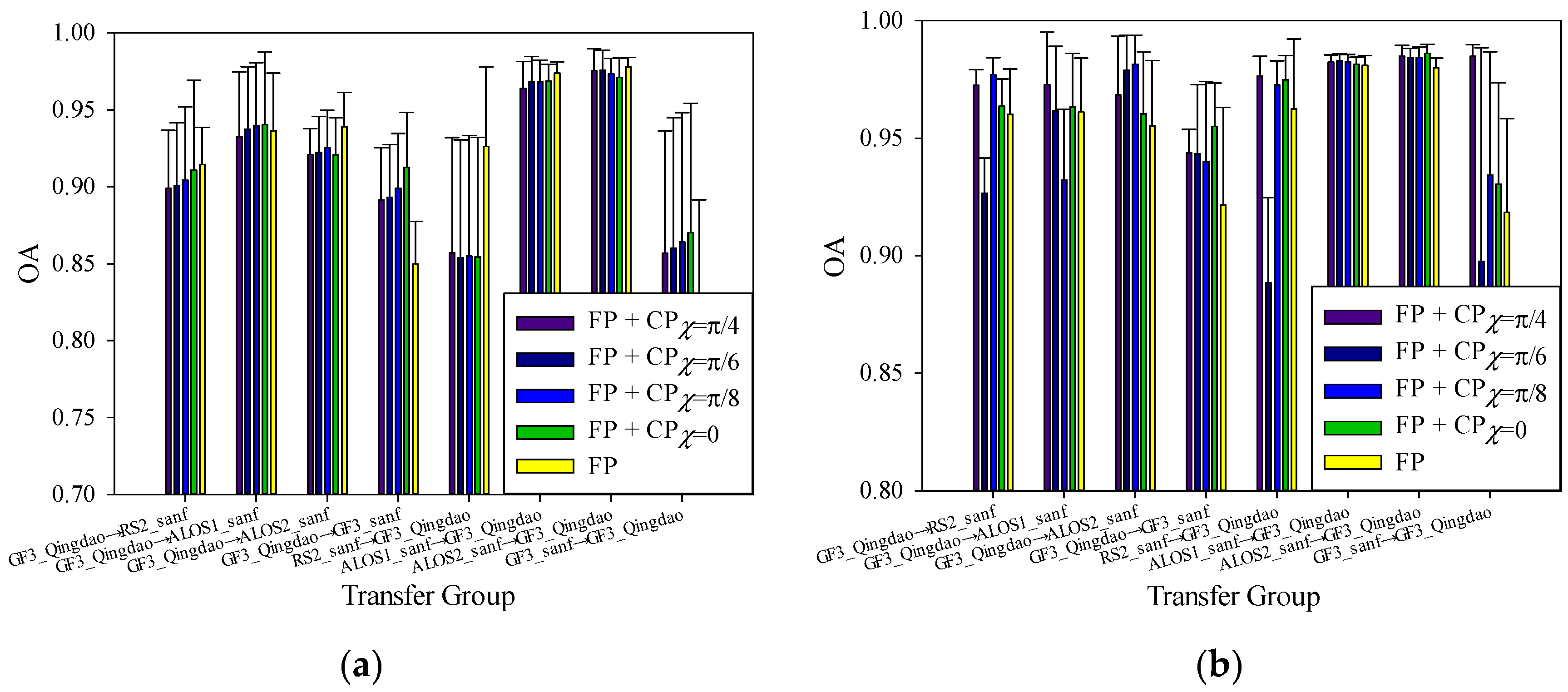
4.2. Cross-Domain Image Classification Based on the FP + GCP SAR Images

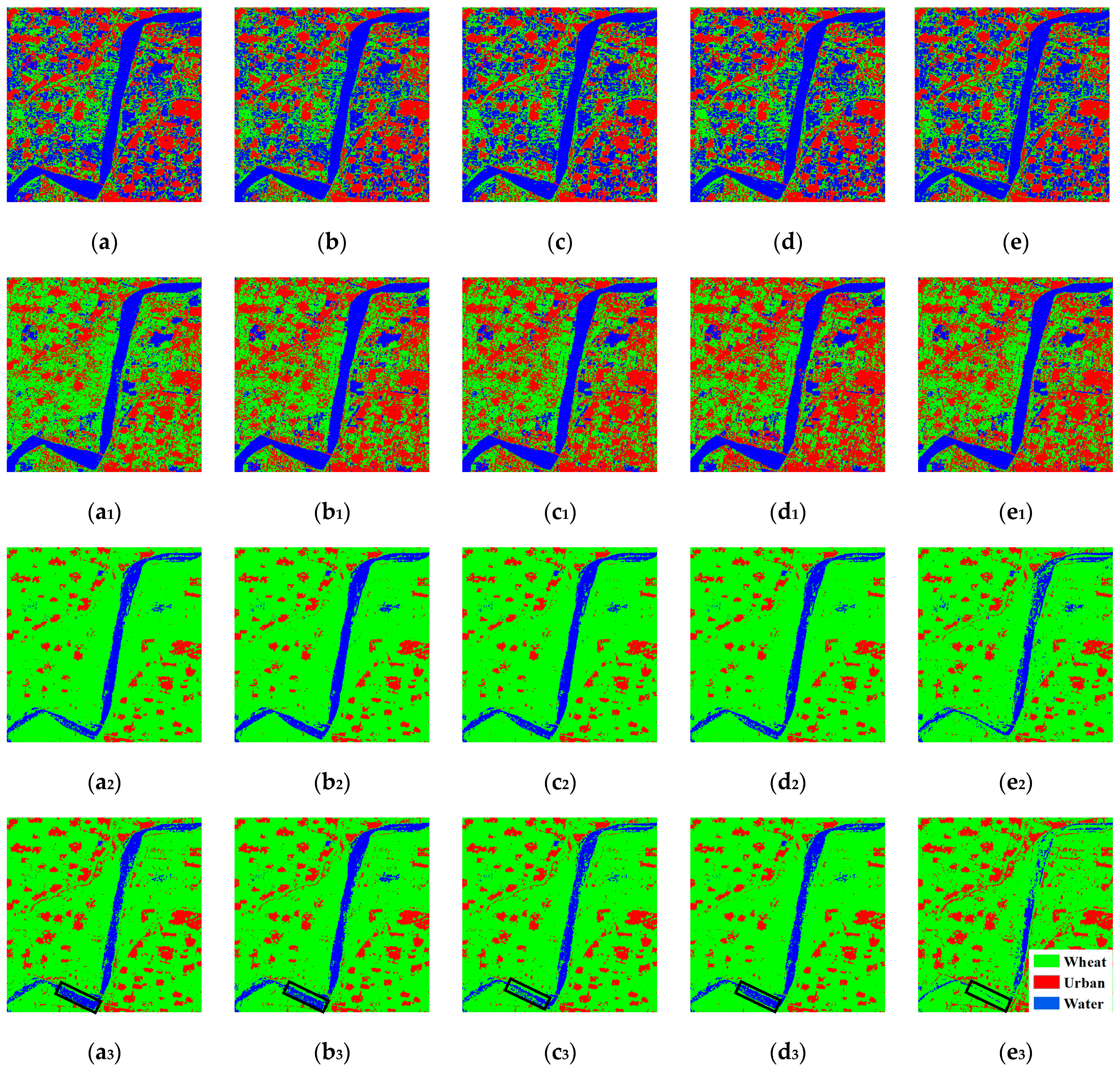
4.2.1. Cross-Scene Image Classification

With the variation in θ and χ, numerous transmitting modes can be acquired from CP SAR data. In the cross-domain classification of FP + GCP data over different areas, we have selected four typical GCP modes, including left circular polarization, two elliptical polarizations, and linear π/4 transmitting polarization waves. In this section, FP SAR data serve as the primary component to construct 44 subsets of polarization feature parameters (FP SAR + GCP SAR) with four typical GCP SAR datasets. The aim is to investigate the potential of various GCP modes for cross-domain classification tasks. As shown in Table 4, the experimental transfer group 3 comprises eight cross-domain image pairs, including five FP SAR data from different radar satellites over the San Francisco and Qingdao areas.

Table 8. The overall accuracy of the cross-domain classification based on the UDA and GFRST-UDA methods for the FP + CP SAR data with circular polarization transmitting.

	GF3 Qingdao→RS2 Sanf	GF3 Qingdao→ALOS1-Sanf	GF3 Qingdao→ALOS2 Sanf	GF3 Qingdao→GF3-Sanf	RS2 Sanf→GF3 Qingdao	ALOS1 Sanf→GF3 Qingdao	ALOS2 Sanf→GF3 Qingdao	GF3 Sanf→GF3 Qingdao
SA	0.886	0.948	0.912	0.874	0.784	0.958	0.976	0.795
GFRST-SA	0.972	0.970	0.962	0.942	0.970	0.980	0.980	0.982
CORAL	0.831	0.852	0.897	0.844	0.794	0.937	0.949	0.802
GFRST-CORAL	0.967	0.937	0.937	0.942	0.979	0.980	0.981	0.984
JDA	0.933	0.960	0.932	0.928	0.885	0.983	0.980	0.908
GFRST-JDA	0.967	0.987	0.985	0.941	0.979	0.986	0.985	0.979
GFK	0.900	0.930	0.910	0.868	0.798	0.953	0.979	0.768
GFRST-GFK	0.971	0.958	0.943	0.952	0.966	0.979	0.982	0.983
BDA	0.931	0.936	0.939	0.922	0.958	0.976	0.978	0.970
GFRST-BDA	0.973	0.990	0.987	0.928	0.975	0.983	0.990	0.988
MEDA	0.912	0.969	0.935	0.912	0.923	0.976	0.991	0.897
GFRST-MEDA	0.985	0.995	0.997	0.957	0.990	0.986	0.991	0.993

shows the overall accuracy of the cross-domain classification based on the UDA and GFRST-UDA methods for the FP + CP SAR (θ = π/4, χ = π/4) data. The GFRST-UDA method yields higher accuracy in cross-domain classification results for each pair compared to the UDA method.

Figure 13 shows the scatter plots of source and target domain feature alignment. From Figure 13b,c, the JDA method enables the conversion of both source and target domains into the same space. Compared to Figure 13b,c alignments, Figure 13b₁,c₁ alignments exhibit better results for water classes. Therefore, the GFRST-JDA method outperforms the JDA method in terms of feature alignment. In Figure 14a–d, the cross-domain image classification of eight cross-domain image pairs is evaluated using FP + GCP SAR parameters with four CP modes, which demonstrated higher accuracy compared to the UDA method. And the overall accuracy is improved by 2–12%.

Figure 15 shows the cross-domain image classification results of eight cross-domain image pairs for the FP + CP SAR (θ = π/4, χ = π/4) data. Comparing Figure 15a,a₁, it can be observed that the GFRST-SA result (Figure 15a₁) outperforms Figure 15a significantly. When San Francisco is considered as the source domain and Qingdao as the target domain, the classification map depicted in Figure 15e₁–h₁ exhibits significantly superior performance compared to that of Figure 15e–h. Particularly in the yellow frame area where the ground truth is water class, there is a phenomenon that Figure 15e–h is misclassified as urban class while Figure 15e₁–h₁ produce accurate classification results. Moreover, Figure 16 shows the overall accuracy of cross-domain classification for four FP + GCP SAR and the FP SAR data, respectively. From Figure 16, it is evident that the classification accuracy of Figure 16b surpasses that of Figure 16a. In comparison to the classification accuracy of the five cases in Figure 16b, the FP + CP SAR (θ = π/4, χ = π/4) based on the GFRST-UDA method can achieve higher classification accuracy in eight cross-domain image pairs with greater stability. This indicates that the circular polarization mode’s CP parameter is advantageous for cross-domain classification.

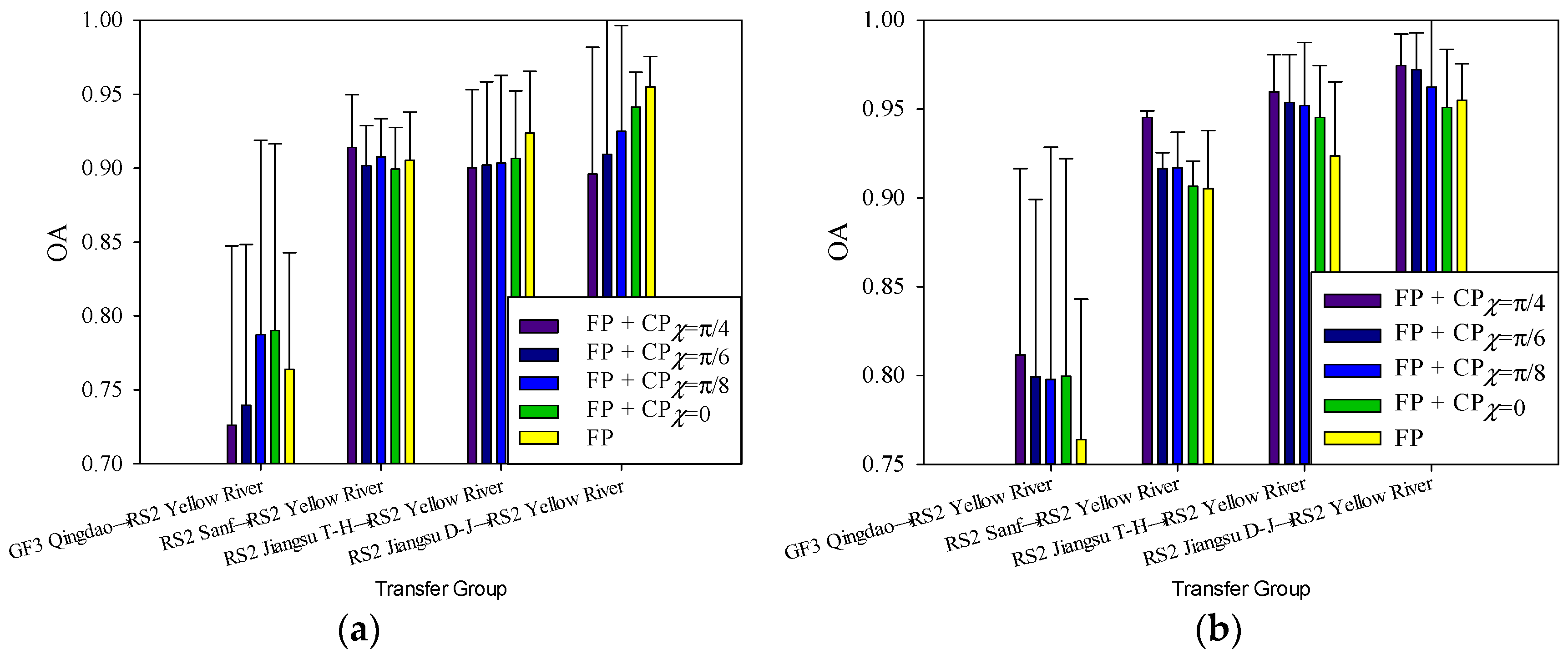
4.2.2. Cross-Crop Type Image Classification

In the study of cross-domain classification of SAR images based on FP + GCP, this section presents detailed experiments on image classification across different crop areas based on the FP + GCP SAR data. As shown in Table 4, the experimental transfer group 4 includes four cross-domain image pairs involving four FP SAR data from different radar satellites in San Francisco, Qingdao, and Jiangsu. Figure 17 shows the overall accuracy statistics of cross-domain classification based on the UDA and GFRST-UDA methods for the FP + GCP SAR data. In Figure 17a–d, the cross-domain image classification of four image pairs is evaluated using FP + GCP SAR parameters with different CP modes based on the GFRST-UDA method, which demonstrated higher accuracy compared to the UDA method. And the overall accuracy was improved by 2–9%.

Comparing cross-domain image classification results maps of the UDA and GFRST-UDA methods, Figure 18 shows cross-domain image classification results. As shown in Figure 18, the classification results of Figure 18a₂,a₃ are significantly superior to those of Figure 18a,a₁. The primary factor lies in the similarity between rice and wheat planting areas, while coastal vegetation exhibits distinct differences from those of wheat areas on radar imagery. Consequently, minimizing scene disparities in cross-domain image classification enhances feature alignment efficacy and elevates classification accuracy. Taking the RS-2 Jiangsu D-J→RS-2 Yellow River cross-domain pair as an example, this study compares the classification results of cross-domain images based on the GFRST-UDA method using four sets of the FP + GCP SAR data. The cross-domain image classification map for the FP + CP SAR (θ = π/4, χ = π/4) outperforms those for the FP + CP SAR (θ = π/4, χ = π/6), the FP + CP SAR (θ = π/4, χ = π/8), and the FP + CP SAR (θ = π/4, χ = 0), as illustrated in Figure 18a₃–e₃. Furthermore, the classification results are significantly better than the cross-domain image classification maps obtained by solely using the FP SAR data. Especially in the black frame area, the ground truth of the black frame is that it represents pure water. Figure 18a₃ is correctly identified as water class. However, Figure 18b₃–e₃ are mistakenly classified as wheat instead of water.

Moreover, Figure 19 shows the overall accuracy of cross-domain classification for the FP + CP SAR and the FP SAR data, respectively. As depicted in Figure 19, the classification accuracy of Figure 19b surpasses that of Figure 19a. In comparison to the classification accuracy of the five cases in Figure 19b, the FP + CP SAR (θ = π/4, χ = π/4) based on the GFRST-UDA method can achieve higher classification accuracy in four cross-domain image pairs with greater stability. Similarly, this indicates that the circular polarization mode’s CP parameter is advantageous for cross-domain classification.

In addition, the RS2 Jiangsu D-J→RS2 Yellow River and RS2 Jiangsu T-H→RS2 Yellow River exhibit superior cross-domain classification accuracy compared to GF3 Qingdao→RS2 Yellow River and RS2 Sanf→RS2 Yellow River. Furthermore, the cross-domain classification accuracy of RS2 Jiangsu D-J→RS2 Yellow River is marginally higher than that of RS2 Jiangsu T-H→RS2 Yellow River. This is because the planting scene of D-J is more analogous to that of wheat. The radar image of the rice planting area was acquired on 16 September, during the Heading–Flowering stage of the rice phenological period, as depicted in Figure 2a,b. Moreover, D-J exhibited a longer growth cycle than T-H and had a shorter plant height than T-H. For the wheat planting area, we acquired an image on 31 March during the regreening–elongation stage of the phenological period. The plants were observed to be shorter, as depicted in Figure 3a. As a consequence of this, the planting scene of D-J rice is more akin to that of wheat, resulting in similar polarization scattering characteristics on radar images and promoting higher cross-domain classification accuracy. Therefore, the degree of scene similarity has a certain impact on the accuracy of cross-domain crop classification based on GCP SAR data. When the cross-domain scenes are more similar, higher accuracy can be achieved in cross-domain classification.

In this study, the feature contribution threshold employed in the GRFST method is selected based on empirical considerations. To investigate the generalizability of the feature contribution threshold on cross-domain classification results, we explore its impact on the accuracy of cross-domain classification by varying the size of the threshold. The study found that when the empirical contribution threshold is around 95%, the classification results of transferring from the source domain to the target domain are the best. At this threshold level, both domains retain the majority of relevant features while effectively eliminating redundant ones. Consequently, the proposed method finds efficacious features across domains, enhancing the overall performance of cross-domain classification.

In addition, we compared different feature alignment methods, as shown in Table 6. In general, GFRST-MEDA has the best classification effect after feature alignment. The reason is that the MEDA method uses manifold feature learning to solve the deteriorating feature representation problem. Then, it realizes dynamic distribution alignment; that is, the adaptation factor dynamically adjusts the weights aligned between the edge probability distribution and the conditional probability distribution. And MEDA also retains meaningful semantic relationships. One of this study’s important purposes is to use the GFRST method to optimize the polarization features and then classify the optimal features to obtain a better classification result.

5. Conclusions

This study proposes a novel unsupervised classification method with the aim to address two challenges in unsupervised cross-domain image classification, and for the first time, the performances of various CP SAR modes for cross-domain terrain type classification are evaluated. The method is validated from different cross-domain scenarios, including cross-data source, cross-scene, and cross-crop type on the GCP SAR data.

It is found that the optimal CP features (g₀, σ_CR, σ_CH, Pd_m-α_s, Pv_m-δ, and Pv_m-χ) can describe the target stably under different scenarios, thereby improving the cross-domain classification accuracy. In the cross-domain classification from images with different sensors over the same area, based on the proposed method, the classification accuracy is above 85%, which is 8% higher than that of the UDA method since the cross-domain feature distribution shift is much alleviated. Moreover, for the cross-domain classification from images acquired over different scenes, the proposed method yields classification results with an accuracy of 3% to 5% higher than that of the UDA method. In polarimetric SAR terrain type classification, most studies only consider the FP information and do not consider other partial polarimetric information, such as the CP information. By combining FP and CP features, especially the circular CP mode (θ = π/4, χ = π/4), the classification accuracy of cross-domain terrain type can be steadily improved. In addition, in cross-crop type image classification based on the FP + GCP SAR images, it is found that the degree of scene similarity affects the classification accuracy.

References

1. Yamaguchi, Y.; Sato, A.; Boerner, W.M.; Sato, R.; Yamada, H. Four-component scattering power decomposition with rotation of coherency matrix. IEEE Trans. Geosci. Remote Sens. 2011, 49, 2251–2258. [Google Scholar] [CrossRef]
2. Souyris, J.C.; Imbo, P.; Fjortoft, R.; Mingot, S.; Lee, J.S. Compact polarimetry based on symmetry properties of geophysical media: The/spl pi//4 mode. IEEE Trans. Geosci. Remote Sens. 2005, 43, 634–646. [Google Scholar] [CrossRef]
3. Souyris, J.C.; Mingot, S. Polarimetry based on one transmitting and two receiving polarizations: The π/4 mode. In Proceedings of the 2002 IEEE International Geoscience and Remote Sensing Symposium, IGARSS, Toronto, ON, Canada, 24–28 June 2002; pp. 629–631. [Google Scholar]
4. Stacy, N.; Preiss, M. Compact polarimetric analysis of X-band SAR data. In Proceedings of the 6th European Conference on Synthetic Aperture Radar, EUSAR, Dresden, Germany, 16–18 May 2006. [Google Scholar]
5. Raney, R.K. Dual-polarized SAR and stokes parameters. IEEE Geosci. Remote Sens. Lett. 2006, 3, 317–319. [Google Scholar] [CrossRef]
6. Raney, R.K. Hybrid-Polarity SAR Architecture. IEEE Trans. Geosci. Remote Sens. 2007, 45, 3397–3404. [Google Scholar] [CrossRef]
7. Yin, J.; Yang, J. Target Decomposition Based on Symmetric Scattering Model for Hybrid Polarization SAR Imagery. IEEE Geosci. Remote Sens. Lett. 2020, 18, 494–498. [Google Scholar] [CrossRef]
8. Yin, J.; Papathanassiou, K.P.; Yang, J. Formalism of Compact Polarimetric Descriptors and Extension of the ΔαB/αB Method for General Compact-Pol SAR. IEEE Trans. Geosci. Remote Sens. 2019, 57, 10322–10335. [Google Scholar] [CrossRef]
9. Yin, J.; Yang, J.; Zhou, L.; Xu, L. Oil Spill Discrimination by Using General Compact Polarimetric SAR Features. Remote Sens. 2020, 12, 479. [Google Scholar] [CrossRef]
10. Raney, R.K.; Cahil, J.T.S.; Patterson, G.W.; Bussey, D.B.J. The M-Chi decomposition of hybrid dual-polarimetric radar data. In Proceedings of the 2012 IEEE International Geoscience and Remote Sensing Symposium, IGARSS, Munich, Germany, 22–27 July 2012; pp. 5093–5096. [Google Scholar]
11. Charbonneau, F.J.; Brisco, B.; Raney, R.K.; McNairn, H.; Liu, C.; Vachon, P.W.; Shang, J.; DeAbreu, R.; Champagne, C.; Merzouki, A.; et al. Compact polarimetry overview and applications assessment. Can. J. Remote Sens. 2010, 36, S298–S315. [Google Scholar] [CrossRef]
12. Cloude, S.; Goodenough, D.; Chen, H. Compact decomposition theory. IEEE Geosci. Remote Sens. Lett. 2011, 9, 28–32. [Google Scholar] [CrossRef]
13. Guo, X.; Yin, J.; Li, K.; Yang, J. Fine Classification of Rice Paddy Based on RHSI-DT Method Using Multi-Temporal Compact Polarimetric SAR Data. Remote Sens. 2021, 13, 5060. [Google Scholar] [CrossRef]
14. Guo, X.; Yin, J.; Li, K.; Yang, J.; Shao, Y. Scattering Intensity Analysis and Classification of Two Types of Rice Based on Multi-Temporal and Multi-Mode Simulated Compact Polarimetric SAR Data. Remote Sens. 2022, 14, 1644. [Google Scholar] [CrossRef]
15. Gui, R.; Xu, X.; Yang, R.; Wang, L.; Pu, F. Statistical scattering component-based subspace alignment for unsupervised cross-domain PolSAR image classification. IEEE Trans. Geosci. Remote Sens. 2020, 59, 5449–5463. [Google Scholar] [CrossRef]
16. Tuia, D.; Persello, C.; Bruzzone, L. Domain adaptation for the classification of remote sensing data: An overview of recent advances. IEEE Geosci. Remote Sens. Mag. 2016, 4, 41–57. [Google Scholar] [CrossRef]
17. Qin, Y.; Bruzzone, L.; Li, B.; Ye, Y. Cross-domain collaborative learning via cluster canonical correlation analysis and random walker for hyperspectral image classification. IEEE Trans. Geosci. Remote Sens. 2018, 57, 3952–3966. [Google Scholar] [CrossRef]
18. Geng, J.; Deng, X.; Ma, X.; Jiang, W. Transfer learning for SAR image classification via deep joint distribution adaptation networks. IEEE Trans. Geosci. Remote Sens. 2020, 58, 5377–5392. [Google Scholar] [CrossRef]
19. Kouw, W.M.; Loog, M. An Introduction to Domain Adaptation and Transfer Learning. arXiv 2018, arXiv:1812.11806. [Google Scholar]
20. He, D.; Shi, Q.; Liu, X.; Zhong, Y.; Xia, G.; Zhang, L. Generating annual high resolution land cover products for 28 metropolises in China based on a deep super-resolution mapping network using Landsat imagery. GIScience Remote Sens. 2022, 59, 2036–2067. [Google Scholar] [CrossRef]
21. Qin, X.; Yang, J.; Zhao, L.; Li, P.; Sun, K. A Novel Deep Forest-Based Active Transfer Learning Method for PolSAR Images. Remote Sens. 2020, 12, 2755. [Google Scholar] [CrossRef]
22. Wang, M.; Deng, W. Deep visual domain adaptation: A survey. Neurocomputing 2018, 312, 135–153. [Google Scholar] [CrossRef]
23. Dalla Mura, M.; Prasad, S.; Pacifici, F.; Gamba, P.; Chanussot, J. Challenges and opportunities of multimodality and Data Fusion in Remote Sensing. In Proceedings of the 2014 22nd European Signal Processing Conference, EUSIPCO, Lisbon, Portugal, 1–5 September 2014; pp. 106–110. [Google Scholar]
24. Kouw, W.M.; Loog, M. A Review of Domain Adaptation without Target Labels. IEEE Trans. Pattern Anal. Mach. Intell. 2021, 43, 766–785. [Google Scholar] [CrossRef]
25. Kamishima, T.; Hamasaki, M.; Akaho, S. TrBagg: A Simple Transfer Learning Method and its Application to Personalization in Collaborative Tagging. In Proceedings of the 2009 Ninth IEEE International Conference on Data Mining, ICDM, Miami Beach, FL, USA, 6–9 December 2009; pp. 219–228. [Google Scholar]
26. Donahue, J.; Hoffman, J.; Rodner, E.; Saenko, K.; Darrell, T. Semi-supervised Domain Adaptation with Instance Constraints. In Proceedings of the 2013 IEEE Conference on Computer Vision and Pattern Recognition, CVPR, Portland, OR, USA, 23–28 June 2013; pp. 668–675. [Google Scholar]
27. Pereira, L.A.; da Silva Torres, R. Semi-supervised transfer subspace for domain adaptation. Pattern Recognit. 2018, 75, 235–249. [Google Scholar] [CrossRef]
28. Tuia, D.; Pasolli, E.; Emery, W. Using active learning to adapt remote sensing image classifiers. Remote Sens. Environ. 2011, 115, 2232–2242. [Google Scholar] [CrossRef]
29. Matasci, G.; Volpi, M.; Kanevski, M.; Bruzzone, L.; Tuia, D. Semi-supervised transfer component analysis for domain adaptation in remote sensing image classification. IEEE Trans. Geosci. Remote Sens. 2015, 53, 3550–3564. [Google Scholar] [CrossRef]
30. Pan, S.J.; Tsang, I.W.; Kwok, J.T.; Yang, Q. Domain Adaptation via Transfer Component Analysis. IEEE Trans. Neural Netw. 2011, 22, 199–210. [Google Scholar] [CrossRef] [PubMed]
31. Duan, L.; Xu, D.; Tsang, I.W. Domain Adaptation from Multiple Sources: A Domain-Dependent Regularization Approach. IEEE Trans. Neural Netw. Learn. Syst. 2012, 23, 504–518. [Google Scholar] [CrossRef]
32. Othman, E.; Bazi, Y.; Melgani, F.; Alhichri, H.; Alajlan, N.; Zuair, M. Domain Adaptation Network for Cross-Scene Classification. IEEE Trans. Geosci. Remote Sens. 2017, 55, 4441–4456. [Google Scholar] [CrossRef]
33. Zhang, J.; Li, W.; Ogunbona, P. Joint Geometrical and Statistical Alignment for Visual Domain Adaptation. In Proceedings of the 2017 IEEE Conference on Computer Vision and Pattern Recognition, CVPR, Honolulu, HI, USA, 21–26 July 2017; pp. 5150–5158. [Google Scholar]
34. Qin, X.; Yang, J.; Li, P.; Sun, W.; Liu, W. A Novel Relational-Based Transductive Transfer Learning Method for PolSAR Images via Time-Series Clustering. Remote Sens. 2019, 11, 1358. [Google Scholar] [CrossRef]
35. Zhang, W.; Zhu, Y.; Fu, Q. Adversarial deep domain adaptation for multi-band SAR images classification. IEEE Access 2019, 7, 78571–78583. [Google Scholar] [CrossRef]
36. Chen, Z.; Zhao, L.; He, Q.; Kuang, G. Pixel-Level and Feature-Level Domain Adaptation for Heterogeneous SAR Target Recognition. IEEE Geosci. Remote Sens. Lett. 2022, 19, 1–5. [Google Scholar] [CrossRef]
37. Lyu, X.; Qiu, X.; Yu, W.; Xu, F. Simulation-assisted SAR target classification based on unsupervised domain adaptation and model interpretability analysis. J. Radars 2022, 11, 168–182. [Google Scholar]
38. Zhao, S.; Zhang, Z.; Zhang, T.; Guo, W.; Luo, Y. Transferable SAR image classification crossing different satellites under open set condition. IEEE Geosci. Remote Sens. Lett. 2022, 19, 1–5. [Google Scholar] [CrossRef]
39. Dong, H.; Si, L.; Qiang, W.; Miao, W.; Zheng, C.; Wu, Y.; Zhang, L. A Polarimetric Scattering Characteristics-Guided Adversarial Learning Approach for Unsupervised PolSAR Image Classification. Remote Sens. 2023, 15, 1782. [Google Scholar] [CrossRef]
40. Hua, W.; Liu, L.; Sun, N.; Jin, X. A CA_Based Weighted Clustering Adversarial Network for Unsupervised Domain Adaptation PolSAR Image Classification. IEEE Geosci. Remote Sens. Lett. 2023, 20, 1–5. [Google Scholar] [CrossRef]
41. Cloude, S.R.; Pottier, E. An entropy based classification scheme for land applications of polarimetric SAR. IEEE Trans. Geosci. Remote Sens. 1997, 35, 68–78. [Google Scholar] [CrossRef]
42. Guo, R.; Liu, Y.B.; Wu, Y.H.; Zhang, S.X.; Xing, M.D.; He, W. Applying H/α decomposition to compact polarimetric SAR. IET Radar Sonar Navig. 2012, 6, 61–70. [Google Scholar] [CrossRef]
43. Zhang, H.; Xie, L.; Wang, C.; Wu, F.; Zhang, B. Investigation of the capability of H-α decomposition of compact polarimetric SAR. IEEE Geosci. Remote Sens. Lett. 2014, 11, 868–872. [Google Scholar] [CrossRef]
44. Freeman, A.; Durden, S.L. A three-component scattering model for polarimetric SAR data. IEEE Trans. Geosci. Remote Sens. 1998, 36, 963–973. [Google Scholar] [CrossRef]
45. Yin, J.; Yang, J. Symmetric scattering model based feature extraction from general compact polarimetric sar imagery. In Proceedings of the 2020 IEEE International Geoscience and Remote Sensing Symposium, IGARSS, Waikoloa, HI, USA, 26 September–2 October 2020; pp. 1703–1706. [Google Scholar]
46. Yin, J.; Moon, W.M.; Yang, J. Novel model-based method for identification of scattering mechanisms in polarimetric SAR data. IEEE Trans. Geosci. Remote Sens. 2015, 54, 520–532. [Google Scholar] [CrossRef]
47. Yamaguchi, Y.; Moriyama, T.; Ishido, M.; Yamada, H. Four-component scattering model for polarimetric SAR image decomposition. IEEE Trans. Geosci. Remote Sens. 2005, 43, 1699–1706. [Google Scholar] [CrossRef]
48. Chen, S.W.; Wang, X.S.; Sato, M. Uniform polarimetric matrix rotation theory and its applications. IEEE Trans. Geosci. Remote Sens. 2013, 52, 4756–4770. [Google Scholar] [CrossRef]
49. Breiman, L. Random forests. Mach. Learn. 2001, 45, 5–32. [Google Scholar] [CrossRef]
50. Fernando, B.; Habrard, A.; Sebban, M.; Tuytelaars, T. Subspace Alignment For Domain Adaptation. In Proceedings of the 2014 IEEE Conference on Computer Vision and Pattern Recognition, CVPR, Columbus, OH, USA, 23–28 June 2014. [Google Scholar]
51. Long, M.; Wang, J.; Ding, G.; Sun, J.; Yu, P. Transfer feature learning with joint distribution adaptation. In Proceedings of the 2013 IEEE International Conference on Computer Vision, ICCV, Sydney, Australia, 1–8 December 2013; pp. 2200–2207. [Google Scholar]
52. Sun, B.; Feng, J.; Saenko, K. Return of frustratingly easy domain adaptation. In Proceedings of the AAAI Conference on Artificial Intelligence, Phoenix, AZ, USA, 12–17 February 2016. [Google Scholar]
53. Wang, J.; Chen, Y.; Hao, S.; Feng, W.; Shen, Z. Balanced Distribution Adaptation for Transfer Learning. In Proceedings of the 2017 IEEE International Conference on Data Mining, ICDM, New Orleans, LA, USA, 18–21 November 2017; pp. 1129–1134. [Google Scholar]
54. Gong, B.; Shi, Y.; Sha, F.; Grauman, K. Geodesic flow kernel for unsupervised domain adaptation. In Proceedings of the 2012 IEEE Conference on Computer Vision and Pattern Recognition, CVPR, Providence, RI, USA, 16–21 June 2012; pp. 2066–2073. [Google Scholar]
55. Wang, J.; Feng, W.; Chen, Y.; Yu, H.; Huang, M.; Yu, P.S. Visual Domain Adaptation with Manifold Embedded Distribution Alignment. In Proceedings of the 26th ACM international conference on Multimedia, Seoul, Republic of Korea, 22–26 October 2018; pp. 402–410. [Google Scholar]
Figure 1. The Pauli decomposition of FP SAR data ((ad) are SAR images from four radar satellites (RADARSAT-2, ALOS-1, ALOS-2, and GF-3) of San Francisco, respectively. (e) is a SAR image from GF-3 of Qingdao. (f) is a SAR image from RADARSAT-2 of Jiangsu. And (g) is a SAR image from RADARSAT-2 of Yellow River).
Agriculture 14 01511 g001aAgriculture 14 01511 g001b
Figure 2. Field investigation pictures of five kinds of ground objects in Jiangsu ((a) T-H. (b) D-J. (c) urban. (d) shoal. (e) water).
Agriculture 14 01511 g002
Figure 3. Field investigation pictures of three kinds of ground objects in Yellow River ((a) wheat. (b) water. (c) urban).
Agriculture 14 01511 g003
Figure 4. Flow chart of the methodology.
Agriculture 14 01511 g004
Figure 5. Feature importance ranking for source and target domains for CP SAR data with circular polarization transmitting.
Agriculture 14 01511 g005
Figure 6. The overall accuracy of cross-domain classification from SAR satellites with different band channels based on the UDA method for CP SAR data with circular polarization transmitting ((a) SA result. (b) TCA result. (c) JDA result. (d) CORAL result. (e) BDA result. (f) GFK result. (g) MEDA result. (h) MEAN result).
Agriculture 14 01511 g006
Figure 7. The overall accuracy of cross-domain classification for CP SAR data with circular polarization transmitting ((a) mean accuracy of cross-domain image classification. (b) mean accuracy of different SAR frequency bands cross-domain image classification. All CP-UDA: cross-domain classification based on all CP features. GFRS-UDA: cross-domain classification based on Gini coefficient feature ranking only in the source domain. GFRST-UDA: cross-domain classification based on the proposed method. Supervision: supervised classification based on the K-Nearest Neighbor classifier).
Agriculture 14 01511 g007
Figure 8. Cross-domain images (ALOS1-Sanf→GF3-Sanf) classification maps for CP SAR data with circular polarization transmitting ((a) SA result. (b) GFRS-SA result. (c) GFRST-SA result. (d) Supervision result).
Agriculture 14 01511 g008
Figure 9. The scatter plots of source and target domains feature alignment (ad) UJDA scatter plots. (a1d1) GFRS-UJDA scatter plots. (a2d2) GFRST-UJDA scatter plots. (a,a1,a2) scatter plots of the source domain. (b,b1,b2) scatter plots of the aligned source domain. (c,c1,c2) scatter plots of the aligned target domain. (d,d1,d2) scatter plots of the target domain.).
Agriculture 14 01511 g009aAgriculture 14 01511 g009b
Figure 10. The histograms of the dispersion coefficient of source and target domains and aligned source and target domains ((ac) are histograms of dispersion coefficient based on UJDA, GFRS-UJDA, and GFRST-UJDA methods, respectively).
Agriculture 14 01511 g010
Figure 11. The overall accuracy statistics of cross-domain image classification for CP SAR data with circular polarization transmitting.
Agriculture 14 01511 g011
Figure 12. Cross-domain image classification results for CP SAR data with circular polarization transmitting ((ad) (GF3-Qingdao→RS2-sanf) and (a1d1) (ALOS2-sanf→GF3-Qingdao) are cross-domain image classification maps based on SA, GFRS-SA, GFRST-SA, and supervision classification methods, respectively).
Agriculture 14 01511 g012
Figure 13. The scatter plots of source and target domain feature alignment ((ad) JDA scatter plots. (a1d1) GFRST-JDA scatter plots. (a,a1) scatter plots of the source domain. (b,b1) scatter plots of the aligned source domain. (c,c1) scatter plots of the aligned target domain. (d,d1) scatter plots of the target domain).
Agriculture 14 01511 g013
Figure 14. The overall accuracy of cross-domain classification based on the UDA and GFRST-UDA methods for the FP + GCP SAR data ((ad) are overall accuracy for the FP + CP SAR (θ = π/4, χ = π/4), the FP + CP SAR (θ = π/4, χ = π/6), the FP + CP SAR (θ = π/4, χ = π/8), and the FP + CP SAR (θ = π/4, χ = 0), respectively).
Agriculture 14 01511 g014
Figure 15. Cross-domain image classification results for the FP + CP SAR (θ = π/4, χ = π/4) data (ah) SA results. (a1h1) GFRST-SA results. The results from (ah) and from (a1h1) correspond to eight cross-domain pair classification maps, respectively.
Agriculture 14 01511 g015
Figure 16. The overall accuracy statistics of cross-domain classification for the FP + CP SAR and the FP SAR data, respectively ((a) UDA result. (b) GFRST-UDA result).
Agriculture 14 01511 g016
Figure 17. The overall accuracy of cross-domain classification based on the UDA and GFRST-UDA methods for the GCP SAR data (ad) are overall accuracy for the FP + CP SAR (θ = π/4, χ = π/4), the FP + CP SAR (θ = π/4, χ = π/6), the FP + CP SAR (θ = π/4, χ = π/8), and the FP + CP SAR (θ = π/4, χ = 0), respectively.
Agriculture 14 01511 g017
Figure 18. Cross-domain image classification maps for the FP + CP SAR (θ = π/4, χ = π/4), the FP + CP SAR (θ = π/4, χ = π/6), the FP + CP SAR (θ = π/4, χ = π/8), the FP + CP SAR (θ = π/4, χ = 0) and the FP SAR data based on the GFRST-USA method, respectively ((ae,a1e1,a2e2,a3e3) are cross-domain images (GF3 Qingdao, RS2 Sanf, RS2 Jiangsu T-H and RS2 Jiangsu D-J→RS2 Yellow River) results, respectively).
Agriculture 14 01511 g018
Figure 19. The overall accuracy of cross-domain classification for the FP + CP SAR and the FP SAR data, respectively ((a) UDA result. (b) GFRST-UDA result).
Agriculture 14 01511 g019