
Low-Cost Lettuce Height Measurement Based on Depth Vision and Lightweight Instance Segmentation Model


Abstract
1. Introduction
2. Materials and Methods
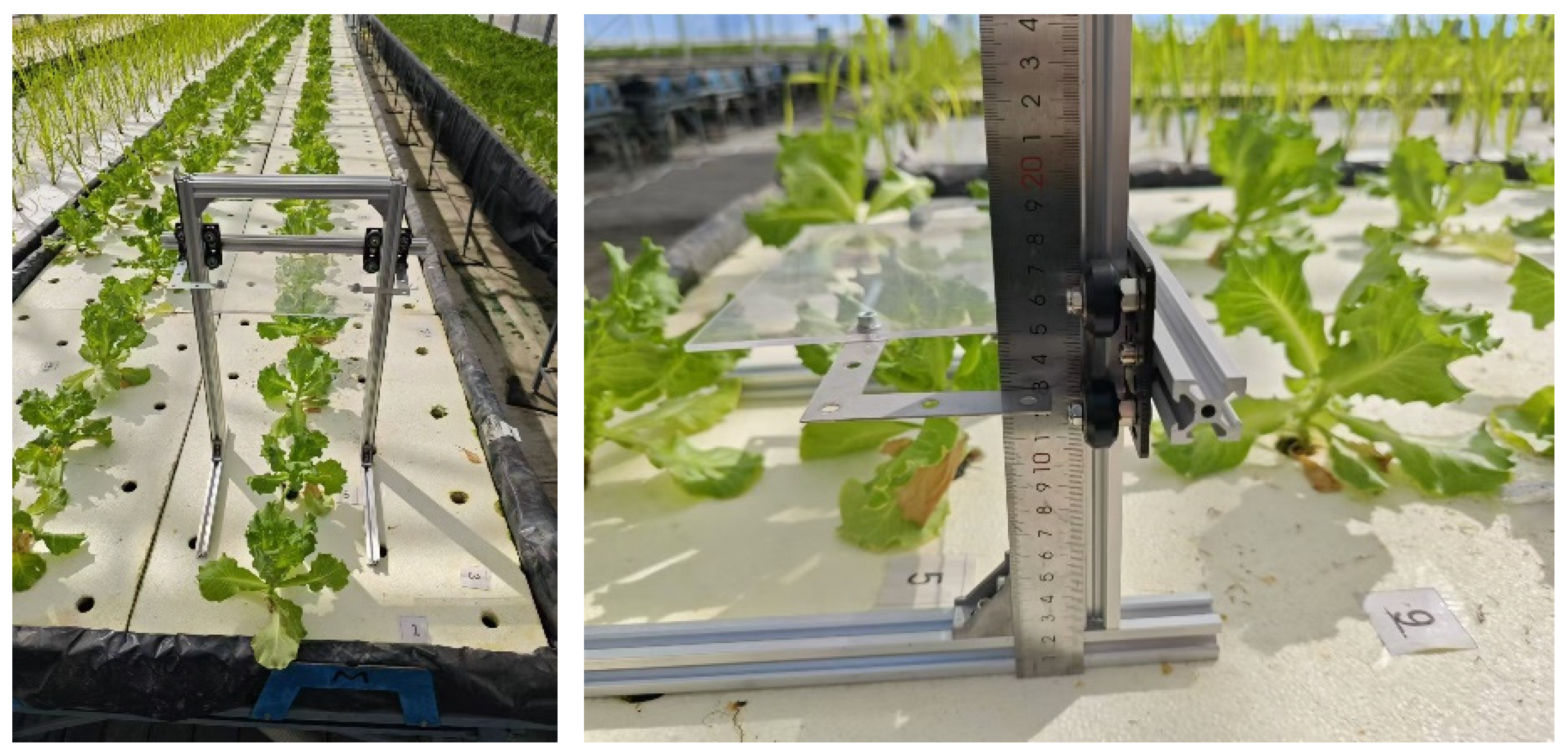
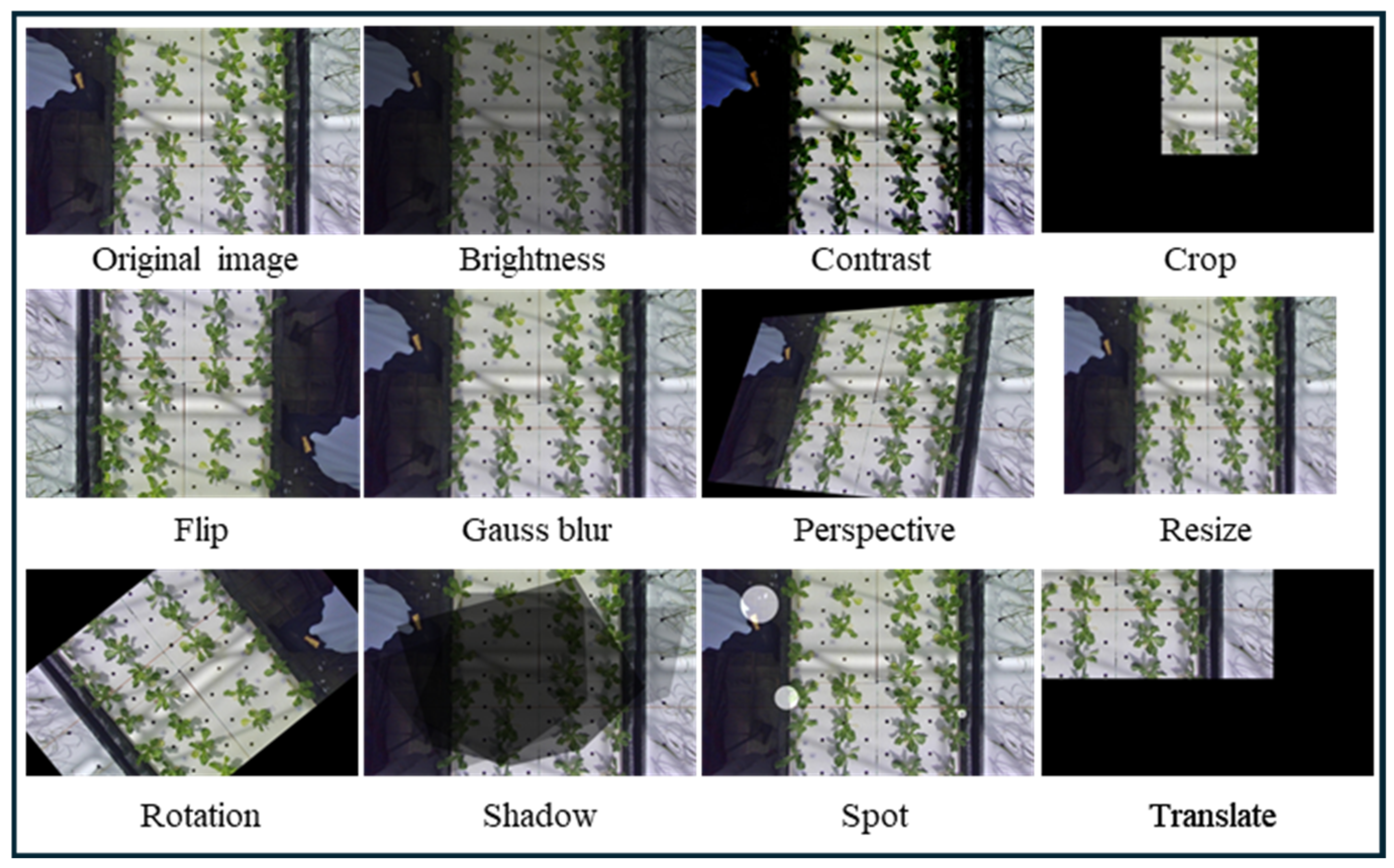
2.1. Data
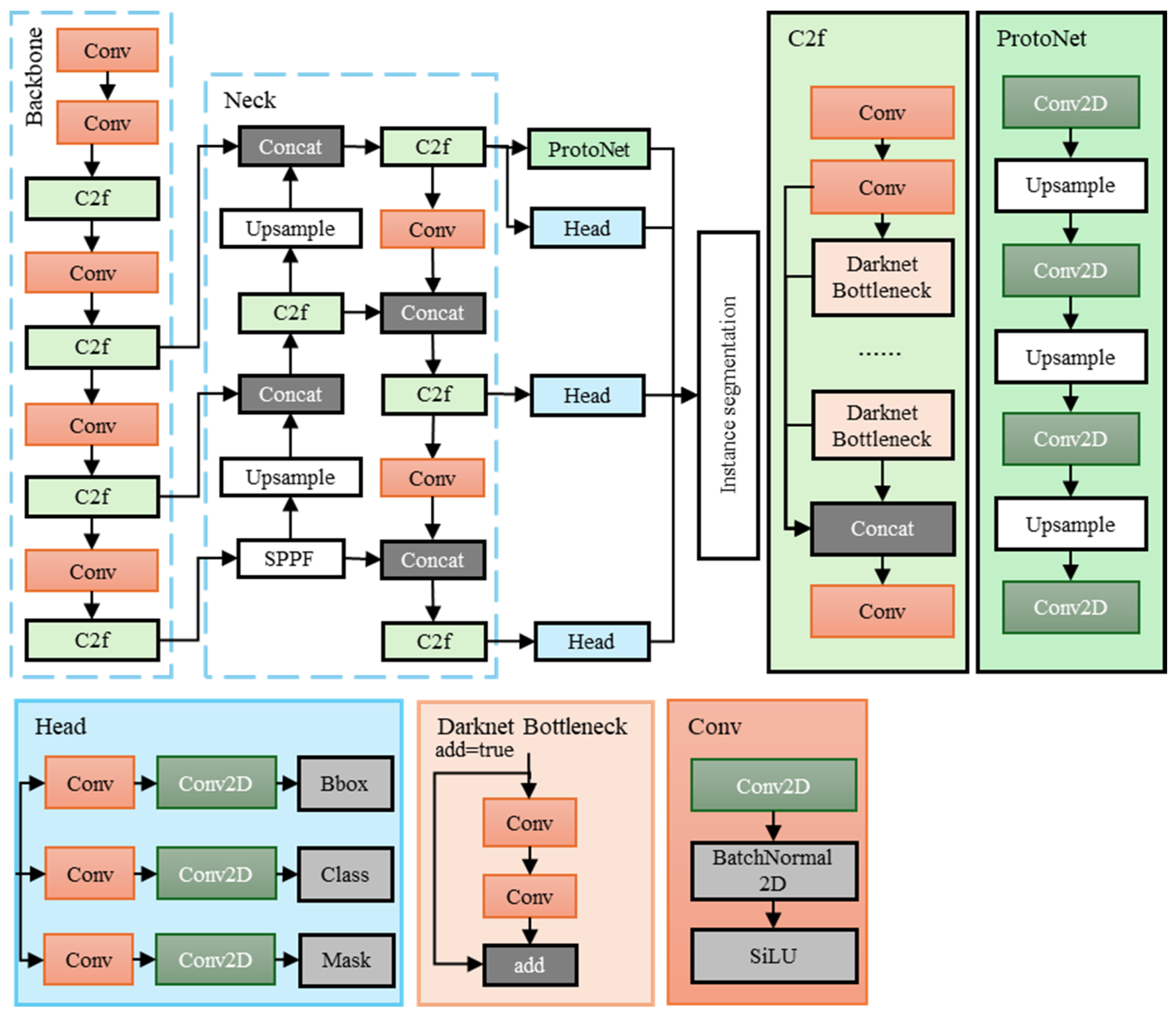
2.2. Lightweight Instance Segmentation Model
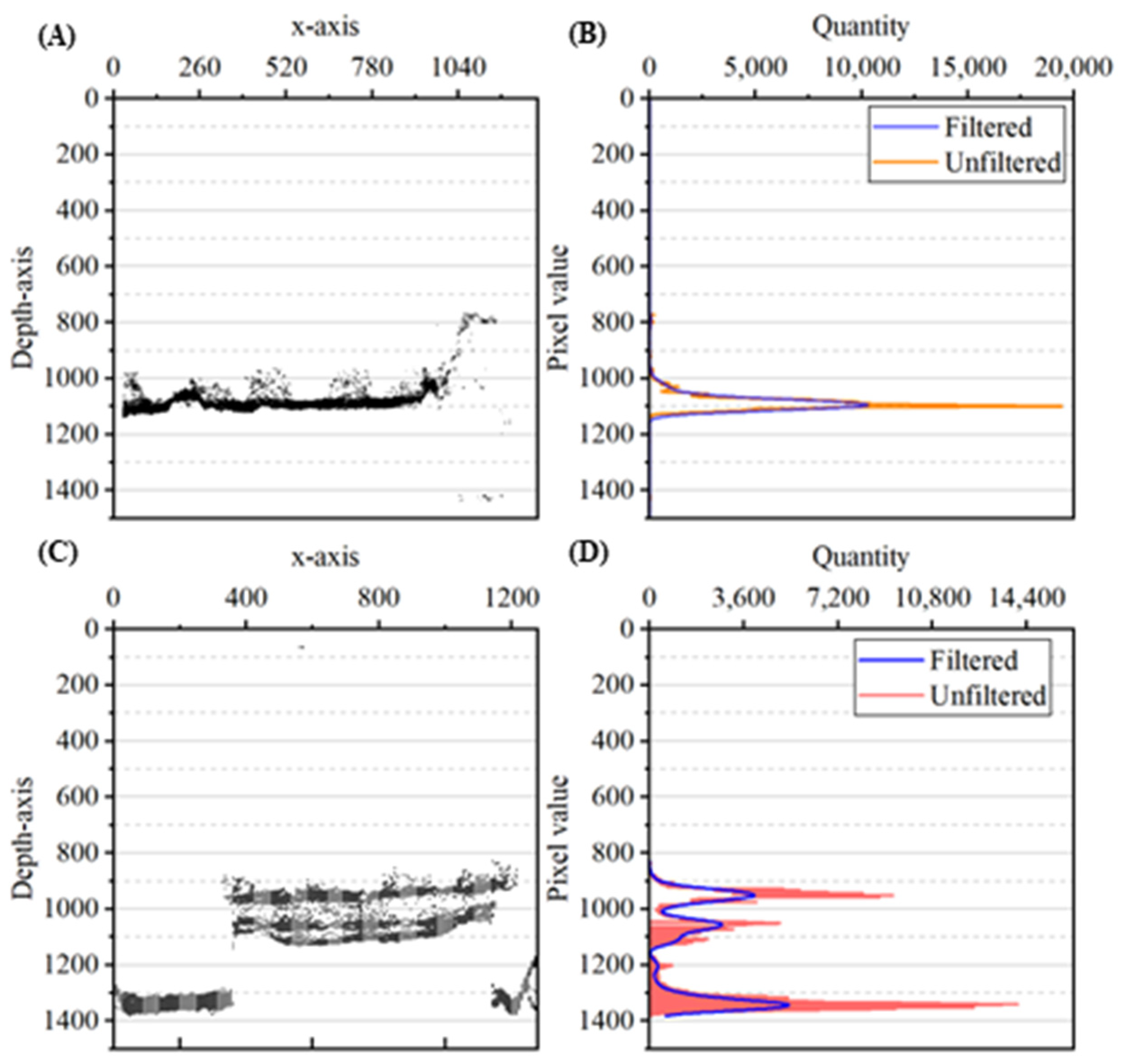
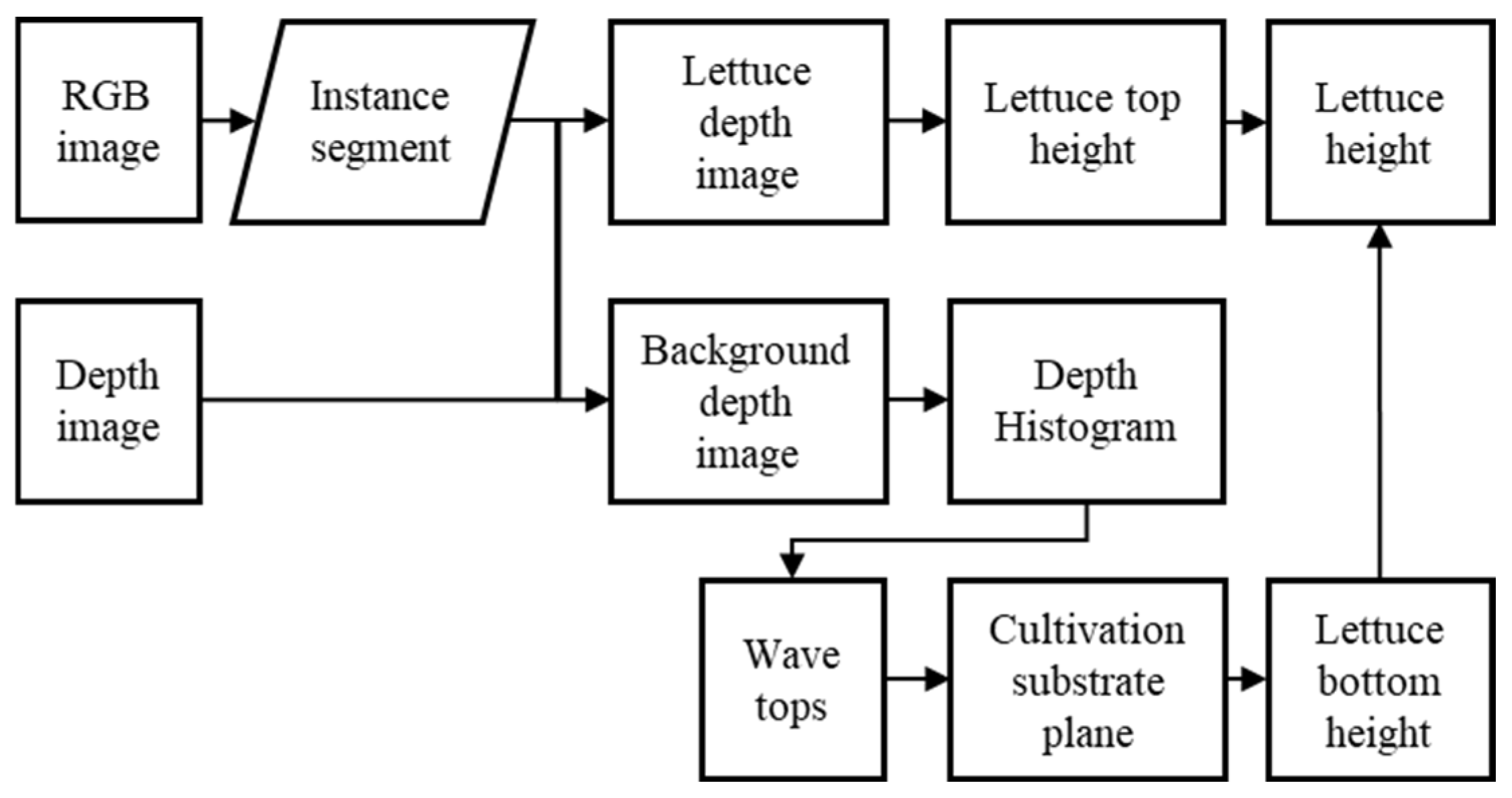
2.3. Measurement of Lettuce Plant Bottom Height
2.4. Multiple Lettuce Height Measurements
3. Experimental Details
3.1. Model Training
3.2. Lettuce Height Measurement Testing
3.3. Evaluation Indicators
4. Results
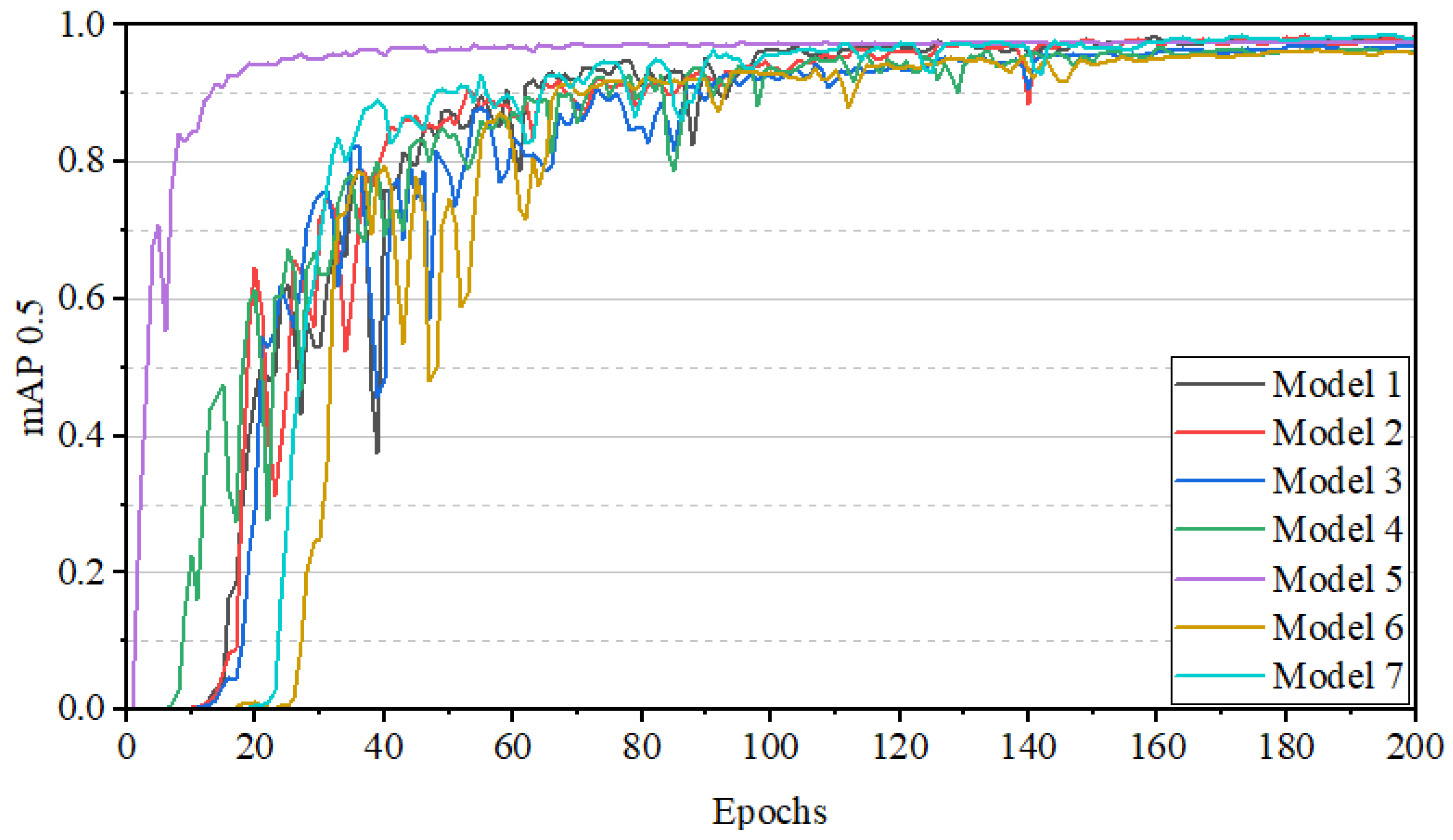
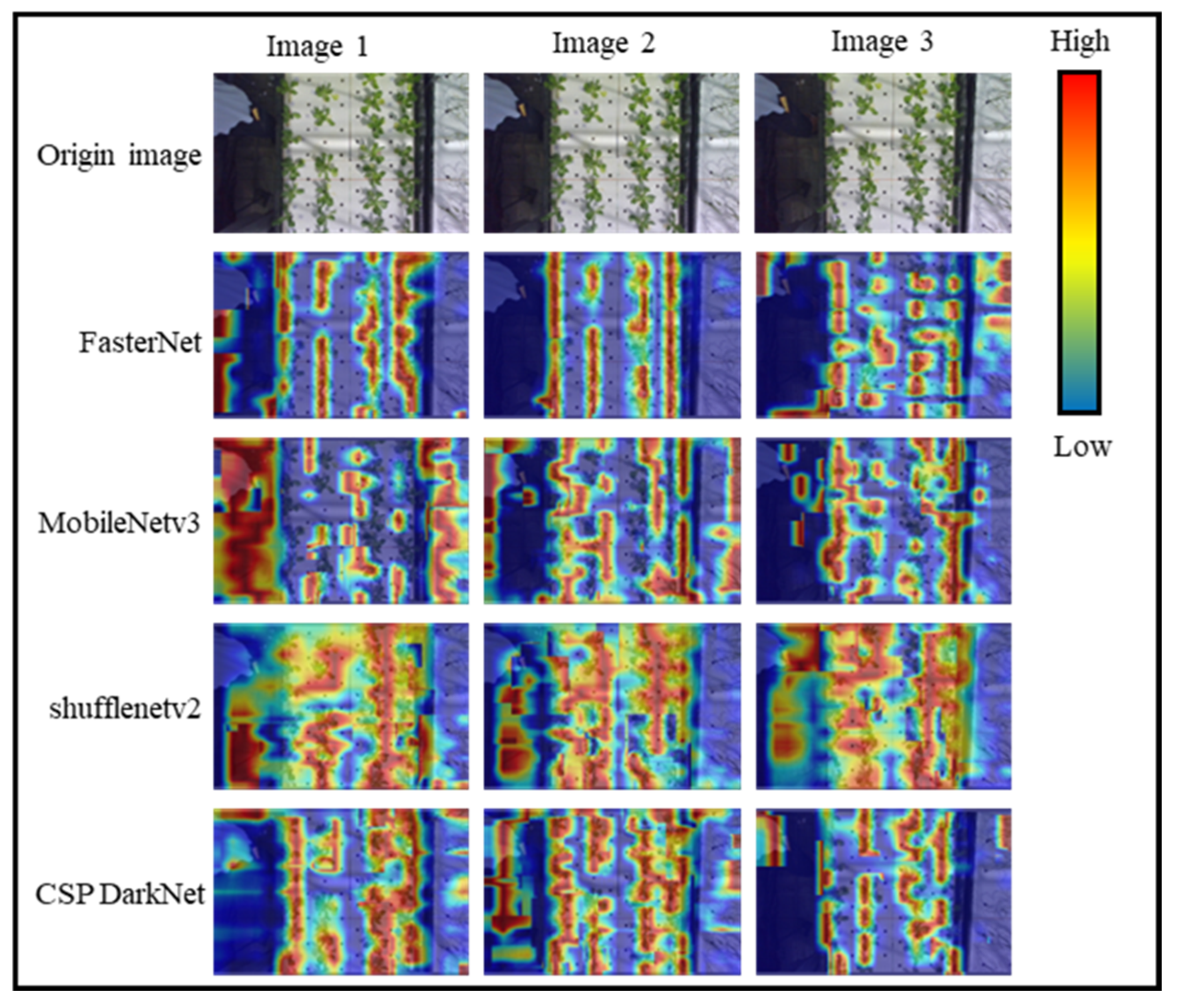
4.1. Instance Segmentation Model Training
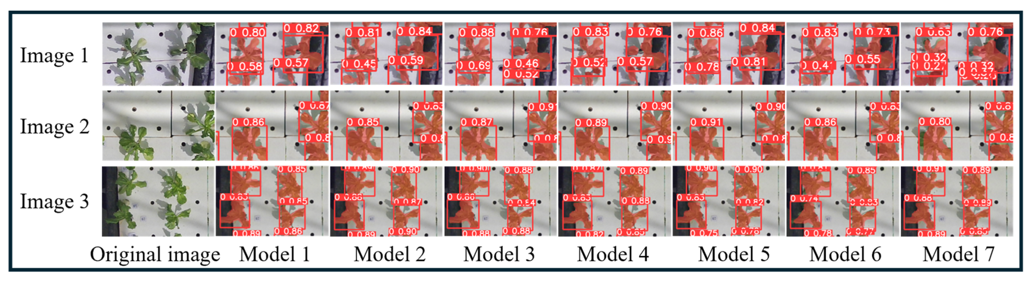
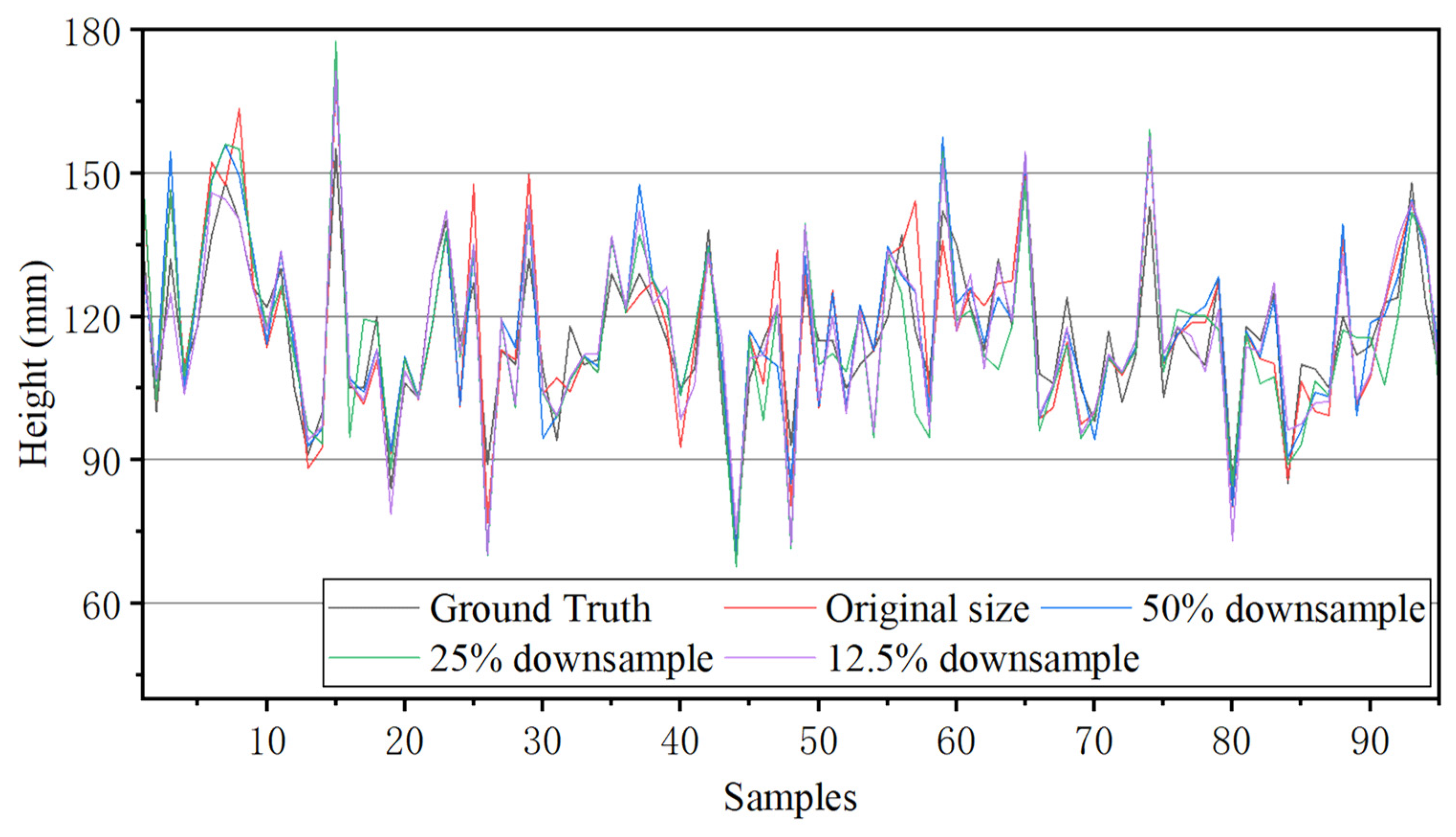
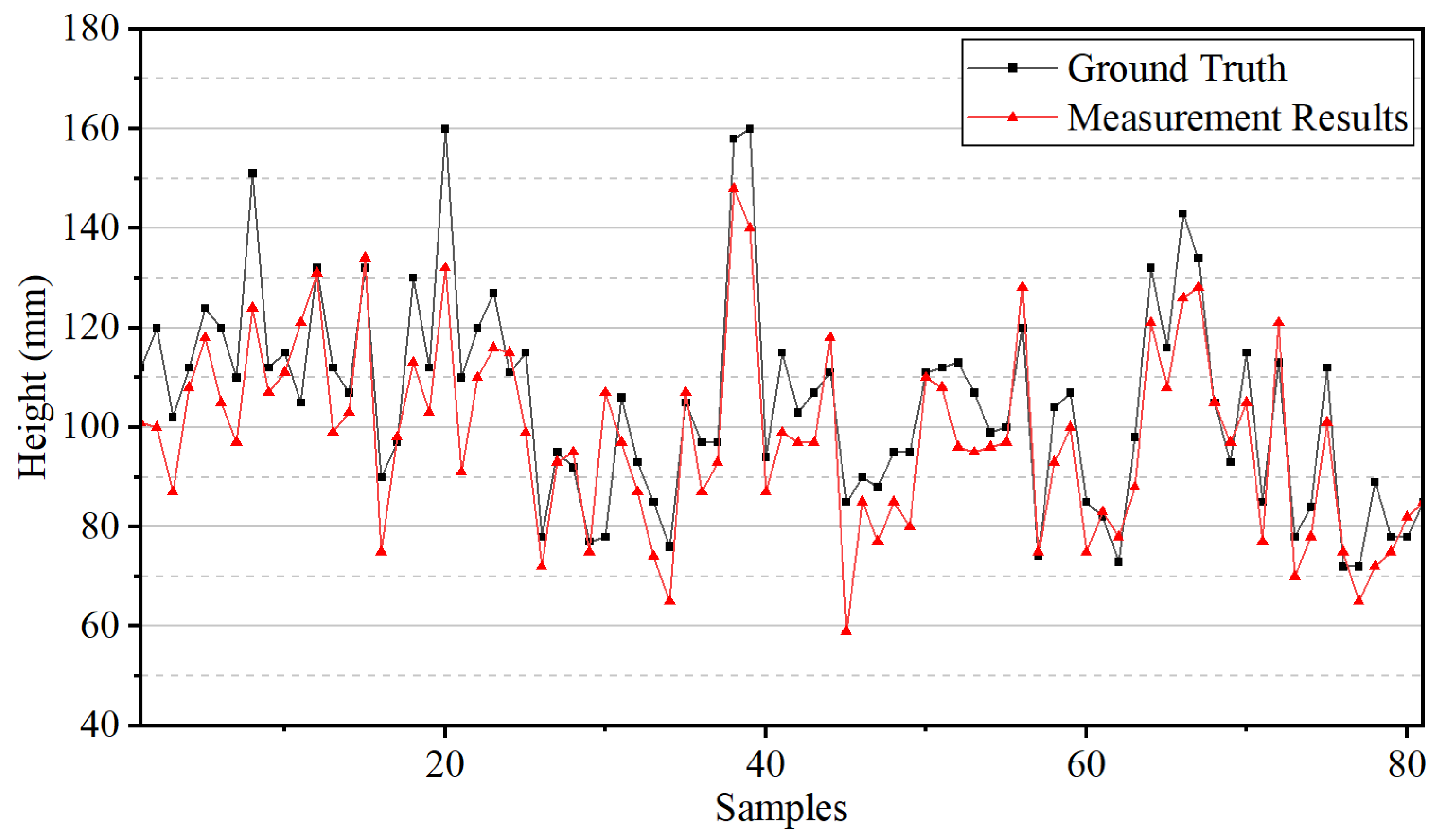
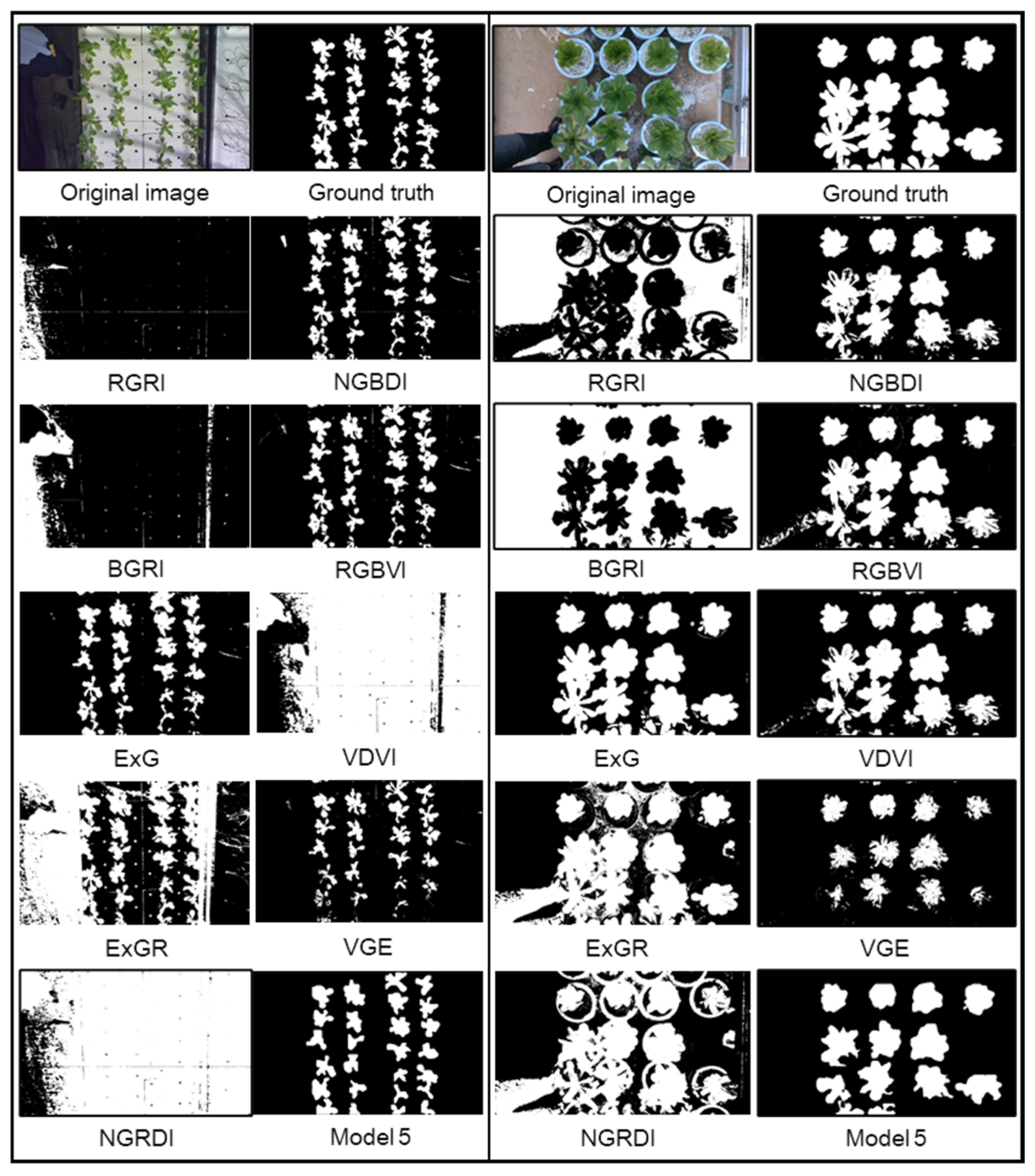
4.2. Plant Height Measurement Results
5. Discussion
- (a)
- Data acquisition improvement: Utilize a mobile acquisition platform to reduce the sensor’s sight distance, thereby enhancing the stability and consistency of the data.
- (b)
- Data optimization: Optimize the original data by increasing the calibration, filtering, and cleaning processes to improve the sensor’s data accuracy.
- (c)
- Engineering optimization: Redesign the engineering construction and deployment processes of deep learning models to further enhance code stability and operational efficiency.
6. Conclusions
Author Contributions
Funding
Institutional Review Board Statement
Data Availability Statement
Acknowledgments
Conflicts of Interest
References
- Petropoulou, A.S.; van Marrewijk, B.; de Zwart, F.; Elings, A.; Bijlaard, M.; van Daalen, T.; Jansen, G.; Hemming, S. Lettuce Production in Intelligent Greenhouses—3D Imaging and Computer Vision for Plant Spacing Decisions. Sensors 2023, 23, 2929. [Google Scholar] [CrossRef] [PubMed]
- Li, H.; Wang, Y.; Fan, K.; Mao, Y.; Shen, Y.; Ding, Z. Evaluation of Important Phenotypic Parameters of Tea Plantations Using Multi-Source Remote Sensing Data. Front. Plant Sci. 2022, 13, 898962. [Google Scholar] [CrossRef] [PubMed]
- Muñoz, M.; Guzmán, J.L.; Sánchez-Molina, J.A.; Rodríguez, F.; Torres, M.; Berenguel, M. A New IoT-Based Platform for Greenhouse Crop Production. IEEE Internet Things J. 2022, 9, 6325–6334. [Google Scholar] [CrossRef]
- Carli, D.; Brunelli, D.; Benini, L.; Ruggeri, M. An Effective Multi-Source Energy Harvester for Low Power Applications. In Proceedings of the 2011 Design, Automation & Test In Europe (Date), Dresden, Germany, 14–18 March 2011; IEEE: Grenoble, France, 2011; pp. 836–841. [Google Scholar]
- Neupane, C.; Pereira, M.; Koirala, A.; Walsh, K.B. Fruit Sizing in Orchard: A Review from Caliper to Machine Vision with Deep Learning. Sensors 2023, 23, 3868. [Google Scholar] [CrossRef]
- Yang, B.; Yang, S.; Wang, P.; Wang, H.; Jiang, J.; Ni, R.; Yang, C. FRPNet: An Improved Faster-ResNet with PASPP for Real-Time Semantic Segmentation in the Unstructured Field Scene. Comput. Electron. Agric. 2024, 217, 108623. [Google Scholar] [CrossRef]
- Rehman, T.U.; Mahmud, M.S.; Chang, Y.K.; Jin, J.; Shin, J. Current and Future Applications of Statistical Machine Learning Algorithms for Agricultural Machine Vision Systems. Comput. Electron. Agric. 2019, 156, 585–605. [Google Scholar] [CrossRef]
- Thakur, A.; Venu, S.; Gurusamy, M. An Extensive Review on Agricultural Robots with a Focus on Their Perception Systems. Comput. Electron. Agric. 2023, 212, 108146. [Google Scholar] [CrossRef]
- Gai, J.; Tang, L.; Brian, S. Plant Localization and Discrimination Using 2D+3D Computer Vision for Robotic Intra-Row Weed Control. In Proceedings of the 2016 ASABE International Meeting; American Society of Agricultural and Biological Engineers, Orlando, FL, USA, 17 July 2016. [Google Scholar]
- Wang, L.; Zheng, L.; Wang, M. 3D Point Cloud Instance Segmentation of Lettuce Based on PartNet. In Proceedings of the 2022 IEEE/CVF Conference on Computer Vision and Pattern Recognition Workshops (CVPRW), New Orleans, LA, USA, 19–20 June 2022; pp. 1646–1654. [Google Scholar]
- Ji, W.; Pan, Y.; Xu, B.; Wang, J. A Real-Time Apple Targets Detection Method for Picking Robot Based on ShufflenetV2-YOLOX. Agriculture 2022, 12, 856. [Google Scholar] [CrossRef]
- Xu, B.; Cui, X.; Ji, W.; Yuan, H.; Wang, J. Apple Grading Method Design and Implementation for Automatic Grader Based on Improved YOLOv5. Agriculture 2023, 13, 124. [Google Scholar] [CrossRef]
- Hu, T.; Wang, W.; Gu, J.; Xia, Z.; Zhang, J.; Wang, B. Research on Apple Object Detection and Localization Method Based on Improved YOLOX and RGB-D Images. Agronomy 2023, 13, 1816. [Google Scholar] [CrossRef]
- Xu, B.; Fan, J.; Chao, J.; Arsenijevic, N.; Werle, R.; Zhang, Z. Instance Segmentation Method for Weed Detection Using UAV Imagery in Soybean Fields. Comput. Electron. Agric. 2023, 211, 107994. [Google Scholar] [CrossRef]
- Zhang, X.; Li, F.; Zheng, H.; Mu, W. UPFormer: U-Sharped Perception Lightweight Transformer for Segmentation of Field Grape Leaf Diseases. EXPERT Syst. Appl. 2024, 249, 123546. [Google Scholar] [CrossRef]
- Wang, Y.; Yang, L.; Chen, H.; Hussain, A.; Ma, C.; Al-gabri, M. Mushroom-YOLO: A Deep Learning Algorithm for Mushroom Growth Recognition Based on Improved YOLOv5 in Agriculture 4.0. In Proceedings of the 2022 IEEE 20th International Conference on Industrial Informatics (INDIN), Perth, Australia, 25–28 July 2022; pp. 239–244. [Google Scholar]
- Cuong, N.H.H.; Trinh, T.H.; Meesad, P.; Nguyen, T.T. Improved YOLO Object Detection Algorithm to Detect Ripe Pineapple Phase. J. Intell. Fuzzy Syst. 2022, 43, 1365–1381. [Google Scholar] [CrossRef]
- Kose, E.; Cicek, A.; Aksu, S.; Tokatli, C.; Emiroglu, O. Spatio-Temporal Sediment Quality Risk Assessment by Using Ecological and Statistical Indicators: A Review of the Upper Sakarya River, Türkiye. Bull. Environ. Contam. Toxicol. 2023, 111, 38. [Google Scholar] [CrossRef]
- Liu, C.; Gu, B.; Sun, C.; Li, D. Effects of Aquaponic System on Fish Locomotion by Image-Based YOLO v4 Deep Learning Algorithm. Comput. Electron. Agric. 2022, 194, 106785. [Google Scholar] [CrossRef]
- Wang, A.; Qian, W.; Li, A.; Xu, Y.; Hu, J.; Xie, Y.; Zhang, L. NVW-YOLOv8s: An Improved YOLOv8s Network for Real-Time Detection and Segmentation of Tomato Fruits at Different Ripeness Stages. Comput. Electron. Agric. 2024, 219, 108833. [Google Scholar] [CrossRef]
- Wang, C.; Wang, Y.; Liu, S.; Lin, G.; He, P.; Zhang, Z.; Zhou, Y. Study on Pear Flowers Detection Performance of YOLO-PEFL Model Trained With Synthetic Target Images. Front. Plant Sci. 2022, 13, 911473. [Google Scholar] [CrossRef]
- Chen, C.; Zheng, Z.; Xu, T.; Guo, S.; Feng, S.; Yao, W.; Lan, Y. YOLO-Based UAV Technology: A Review of the Research and Its Applications. Drones 2023, 7, 190. [Google Scholar] [CrossRef]
- Dai, G.; Hu, L.; Fan, J. DA-ActNN-YOLOV5: Hybrid YOLO v5 Model with Data Augmentation and Activation of Compression Mechanism for Potato Disease Identification. Comput. Intell. Neurosci. 2022, 2022, e6114061. [Google Scholar] [CrossRef]
- Bai, B.; Wang, J.; Li, J.; Yu, L.; Wen, J.; Han, Y. T-YOLO: A Lightweight and Efficient Detection Model for Nutrient Buds in Complex Tea-plantation Environments. J. Sci. Food Agric. 2024, 104, 5698–5711. [Google Scholar] [CrossRef]
- Shi, H.; Shi, D.; Wang, S.; Li, W.; Wen, H.; Deng, H. Crop Plant Automatic Detecting Based on In-Field Images by Lightweight DFU-Net Model. Comput. Electron. Agric. 2024, 217, 108649. [Google Scholar] [CrossRef]
- Zhang, Z.; Lu, Y.; Zhao, Y.; Pan, Q.; Jin, K.; Xu, G.; Hu, Y. TS-YOLO: An All-Day and Lightweight Tea Canopy Shoots Detection Model. Agronomy 2023, 13, 1411. [Google Scholar] [CrossRef]
- Jiao, Z.; Huang, K.; Jia, G.; Lei, H.; Cai, Y.; Zhong, Z. An Effective Litchi Detection Method Based on Edge Devices in a Complex Scene. Biosyst. Eng. 2022, 222, 15–28. [Google Scholar] [CrossRef]
- Zhu, H.; Lu, Z.; Zhang, C.; Yang, Y.; Zhu, G.; Zhang, Y.; Liu, H. Remote Sensing Classification of Offshore Seaweed Aquaculture Farms on Sample Dataset Amplification and Semantic Segmentation Model. REMOTE Sens. 2023, 15, 4423. [Google Scholar] [CrossRef]
- Xiang, L.; Wang, D. A Review of Three-Dimensional Vision Techniques in Food and Agriculture Applications. Smart Agric. Technol. 2023, 5, 100259. [Google Scholar] [CrossRef]
- Liu, Y.; Yuan, H.; Zhao, X.; Fan, C.; Cheng, M. Fast Reconstruction Method of Three-Dimension Model Based on Dual RGB-D Cameras for Peanut Plant. Plant Methods 2023, 19, 17. [Google Scholar] [CrossRef] [PubMed]
- Stilla, U.; Xu, Y. Change Detection of Urban Objects Using 3D Point Clouds: A Review. ISPRS J. Photogramm. Remote Sens. 2023, 197, 228–255. [Google Scholar] [CrossRef]
- Zhang, Y.; Wu, M.; Li, J.; Yang, S.; Zheng, L.; Liu, X.; Wang, M. Automatic Non-Destructive Multiple Lettuce Traits Prediction Based on DeepLabV3 +. J. Food Meas. Charact. 2023, 17, 636–652. [Google Scholar] [CrossRef]
- Ye, Z.; Tan, X.; Dai, M.; Lin, Y.; Chen, X.; Nie, P.; Ruan, Y.; Kong, D. Estimation of Rice Seedling Growth Traits with an End-to-End Multi-Objective Deep Learning Framework. Front. Plant Sci. 2023, 14, 1165552. [Google Scholar] [CrossRef]
- Zhang, Q.; Zhang, X.; Wu, Y.; Li, X. TMSCNet: A Three-Stage Multi-Branch Self-Correcting Trait Estimation Network for RGB and Depth Images of Lettuce. Front. Plant Sci. 2022, 13, 982562. [Google Scholar] [CrossRef]
- Ma, Y.; Zhang, Y.; Jin, X.; Li, X.; Wang, H.; Qi, C. A Visual Method of Hydroponic Lettuces Height and Leaves Expansion Size Measurement for Intelligent Harvesting. Agronomy 2023, 13, 1996. [Google Scholar] [CrossRef]
- Song, P.; Li, Z.; Yang, M.; Shao, Y.; Pu, Z.; Yang, W.; Zhai, R. Dynamic Detection of Three-Dimensional Crop Phenotypes Based on a Consumer-Grade RGB-D Camera. Front. Plant Sci. 2023, 14, 1097725. [Google Scholar] [CrossRef] [PubMed]
- Grenzdörffer, G.J. Crop Height Determination with UAS Point Clouds. Int. Arch. Photogramm. Remote Sens. Spat. Inf. Sci. 2014, XL-1, 135–140. [Google Scholar] [CrossRef]
- Zhang, Y.; Li, M.; Li, G.; Li, J.; Zheng, L.; Zhang, M.; Wang, M. Multi-Phenotypic Parameters Extraction and Biomass Estimation for Lettuce Based on Point Clouds. Measurement 2022, 204, 112094. [Google Scholar] [CrossRef]
- Hu, Y.; Wang, L.; Xiang, L.; Wu, Q.; Jiang, H. Automatic Non-Destructive Growth Measurement of Leafy Vegetables Based on Kinect. Sensors 2018, 18, 806. [Google Scholar] [CrossRef] [PubMed]
- Malambo, L.; Popescu, S.C.; Murray, S.C.; Putman, E.; Pugh, N.A.; Horne, D.W.; Richardson, G.; Sheridan, R.; Rooney, W.L.; Avant, R.; et al. Multitemporal Field-Based Plant Height Estimation Using 3D Point Clouds Generated from Small Unmanned Aerial Systems High-Resolution Imagery. Int. J. Appl. Earth Obs. Geoinf. 2018, 64, 31–42. [Google Scholar] [CrossRef]
- Hämmerle, M.; Höfle, B. Direct Derivation of Maize Plant and Crop Height from Low-Cost Time-of-Flight Camera Measurements. Plant Methods 2016, 12, 50. [Google Scholar] [CrossRef] [PubMed]
- Song, Y.; Wang, J. Winter Wheat Canopy Height Extraction from UAV-Based Point Cloud Data with a Moving Cuboid Filter. Remote Sens. 2019, 11, 1239. [Google Scholar] [CrossRef]
- Qiu, R.; Zhang, M.; He, Y. Field Estimation of Maize Plant Height at Jointing Stage Using an RGB-D Camera. Crop J. 2022, 10, 1274–1283. [Google Scholar] [CrossRef]
- Xia, S.; Chen, D.; Wang, R.; Li, J.; Zhang, X. Geometric Primitives in LiDAR Point Clouds: A Review. IEEE J. Sel. Top. Appl. Earth Obs. Remote Sens. 2020, 13, 685–707. [Google Scholar] [CrossRef]
- Jin, Z.; Tillo, T.; Zou, W.; Zhao, Y.; Li, X. Robust Plane Detection Using Depth Information From a Consumer Depth Camera. IEEE Trans. Circuits Syst. Video Technol. 2019, 29, 447–460. [Google Scholar] [CrossRef]
- Gupta, C.; Tewari, V.K.; Machavaram, R.; Shrivastava, P. An Image Processing Approach for Measurement of Chili Plant Height and Width under Field Conditions. J. Saudi Soc. Agric. Sci. 2022, 21, 171–179. [Google Scholar] [CrossRef]
- Guo, X.; Guo, Q.; Feng, Z. Detecting the Vegetation Change Related to the Creep of 2018 Baige Landslide in Jinsha River, SE Tibet Using SPOT Data. Front. Earth Sci. 2021, 9. [Google Scholar] [CrossRef]
- Chen, J.; Kao, S.; He, H.; Zhuo, W.; Wen, S.; Lee, C.-H.; Chan, S.-H.G. Run, Don’t Walk: Chasing Higher FLOPS for Faster Neural Networks. In Proceedings of the 2023 IEEE/CVF Conference on Computer Vision and Pattern Recognition (CVPR), Vancouver, BC, Canada, 18–22 June 2023; pp. 12021–12031. [Google Scholar]
- Han, D.; Yun, S.; Heo, B.; Yoo, Y. Rethinking Channel Dimensions for Efficient Model Design. In Proceedings of the 2021 IEEE/CVF Conference on Computer Vision and Pattern Recognition (CVPR), Nashville, TN, USA, 20–25 June 2021; pp. 732–741. [Google Scholar]
- Chen, R.; Han, L.; Zhao, Y.; Zhao, Z.; Liu, Z.; Li, R.; Xia, L.; Zhai, Y. Extraction and Monitoring of Vegetation Coverage Based on Uncrewed Aerial Vehicle Visible Image in a Post Gold Mining Area. Front. Ecol. Evol. 2023, 11, 1171358. [Google Scholar] [CrossRef]
- Otsu, N. A Threshold Selection Method from Gray-Level Histograms. IEEE Trans. Syst. Man Cybern. 1979, 9, 62–66. [Google Scholar] [CrossRef]
- Sezgin, M.; Sankur, B. Survey over Image Thresholding Techniques and Quantitative Performance Evaluation. J. Electron. Imaging 2004, 13, 146–165. [Google Scholar] [CrossRef]
- Liu, W.; Li, Y.; Liu, J.; Jiang, J. Estimation of Plant Height and Aboveground Biomass of Toona Sinensis under Drought Stress Using RGB-D Imaging. Forests 2021, 12, 1747. [Google Scholar] [CrossRef]
- Bahman, L. Height Measurement of Basil Crops for Smart Irrigation Applications in Greenhouses Using Commercial Sensors. Master’s Thesis, The University of Western Ontario, London, ON, Canada, 2019. [Google Scholar]


| Orbbec Gemini 336L | Realsense D435 | |
|---|---|---|
| Application scene | Hydroponics | Potting |
| Spatial error | <0.8% at 2 m | <2% at 2 m |
| Resolution | 1280 × 800 | 1280 × 720 |
| Field of view | 90° × 65° | 87° × 58° |
| Frame rate | 30 | 30 |
| Type | Parameters |
|---|---|
| Brightness | It = φB × I, φ ∈ [0.5–1] |
| Contrast | ICt = (255 × φCt)/(1 + eI−128), φCt ∈ [16, 32] |
| Crop | Acr = φCr × A, φCr ∈ [0.1, 1] |
| Flip | One of left–right or up–down flipping, or both. |
| Gauss blur | Kernel size in [3, 9] pixels. |
| Perspective | X-axis and y-axis transform angles are in the range of [−60, 60] degrees with a step size of 1. |
| Resize | X-axis and y-axis transform scales are in the range of [0.5, 1.5]. |
| Rotation | Rotation angle of [0, 359] degrees with the step size of 1. |
| Shadow | Shadow contours number in [1, 3]. |
| Spot | Spot number in [1, 10], spot size in [0, 160] pixels, transparency in [0.5, 0.7]. |
| Translate | X-axis and y-axis transform scale range of [−0.5, 0.5]. |
| Dataset | Total No. of Images | No. Images in Training Set | No. Images in Val Set | Train Targets | Val Targets | Random Transform |
|---|---|---|---|---|---|---|
| Dataset 1 | 80 | 60 | 20 | 1530 | 559 | None |
| Dataset 2 | 80 | 60 | 20 | 1378 | 388 | 11 types |
| Dataset 3 | 880 | 660 | 220 | 15,572 | 5727 | 11 types |
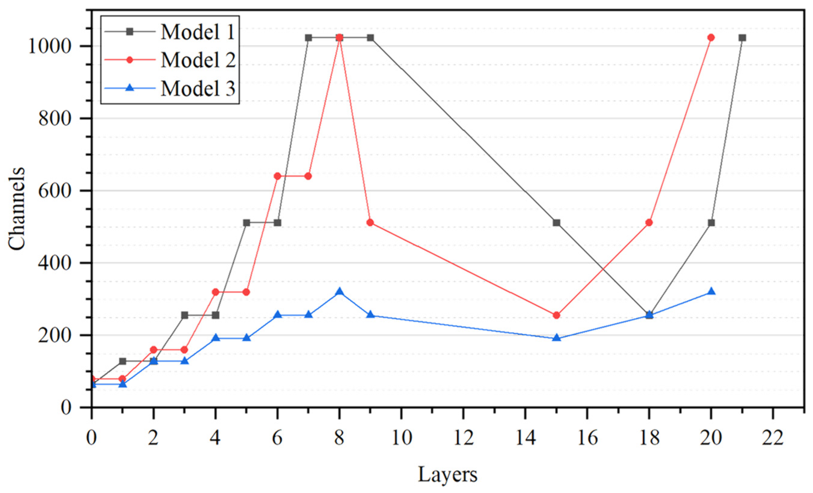
| Model | Dataset | Backbone | Channel Dimension Growth Relationships |
|---|---|---|---|
| Model 1 | Dataset 1 | CSP DarkNet | +2n |
| Model 2 | Dataset 1 | FasterNet T0 | +2n |
| Model 3 | Dataset 1 | FasterNet T0 | +16 |
| Model 4 | Dataset 2 | FasterNet T0 | +16 |
| Model 5 | Dataset 3 | FasterNet T0 | +16 |
| Model 6 | Dataset 1 | MobileNetv3 | Unmodified |
| Model 7 | Dataset 1 | ShuffleNetv2 | Unmodified |
| Model | P | R | mAP0.5 | Inference Time (s) | Parameters (M) | GFLOPs |
|---|---|---|---|---|---|---|
| Model 1 | 0.951 | 0.963 | 0.977 | 0.054 | 3.258 | 11.973 |
| Model 2 | 0.935 | 0.961 | 0.982 | 0.054 | 3.158 | 11.568 |
| Model 3 | 0.967 | 0.922 | 0.981 | 0.040 | 1.369 | 5.960 |
| Model 4 | 0.962 | 0.957 | 0.989 | 0.039 | 1.369 | 5.960 |
| Model 5 | 0.998 | 0.985 | 0.995 | 0.040 | 1.369 | 5.960 |
| Model 6 | 0.916 | 0.937 | 0.973 | 0.058 | 3.749 | 14.679 |
| Model 7 | 0.969 | 0.947 | 0.986 | 0.061 | 2.502 | 10.383 |
| Downsampling Ratios (Length of Side) | Pixels in Image | Instance Segmentation Time (s) | Height Measurement Time (s) | Time for All (s) | Average Accuracy | R2 |
|---|---|---|---|---|---|---|
| 1 | 921,600 | 0.071 | 0.748 | 0.818 | 93.666% | 0.882 |
| 0.7 | 451,584 | 0.075 | 0.307 | 0.381 | 94.115% | 0.902 |
| 0.5 | 230,400 | 0.067 | 0.172 | 0.239 | 93.464% | 0.876 |
| 0.354 | 115,491 | 0.070 | 0.073 | 0.143 | 94.339% | 0.907 |
Disclaimer/Publisher’s Note: The statements, opinions and data contained in all publications are solely those of the individual author(s) and contributor(s) and not of MDPI and/or the editor(s). MDPI and/or the editor(s) disclaim responsibility for any injury to people or property resulting from any ideas, methods, instructions or products referred to in the content. |
© 2024 by the authors. Licensee MDPI, Basel, Switzerland. This article is an open access article distributed under the terms and conditions of the Creative Commons Attribution (CC BY) license (https://creativecommons.org/licenses/by/4.0/).
Share and Cite
Zhao, Y.; Zhang, X.; Sun, J.; Yu, T.; Cai, Z.; Zhang, Z.; Mao, H. Low-Cost Lettuce Height Measurement Based on Depth Vision and Lightweight Instance Segmentation Model. Agriculture 2024, 14, 1596. https://doi.org/10.3390/agriculture14091596
Zhao Y, Zhang X, Sun J, Yu T, Cai Z, Zhang Z, Mao H. Low-Cost Lettuce Height Measurement Based on Depth Vision and Lightweight Instance Segmentation Model. Agriculture. 2024; 14(9):1596. https://doi.org/10.3390/agriculture14091596
Chicago/Turabian StyleZhao, Yiqiu, Xiaodong Zhang, Jingjing Sun, Tingting Yu, Zongyao Cai, Zhi Zhang, and Hanping Mao. 2024. "Low-Cost Lettuce Height Measurement Based on Depth Vision and Lightweight Instance Segmentation Model" Agriculture 14, no. 9: 1596. https://doi.org/10.3390/agriculture14091596
APA StyleZhao, Y., Zhang, X., Sun, J., Yu, T., Cai, Z., Zhang, Z., & Mao, H. (2024). Low-Cost Lettuce Height Measurement Based on Depth Vision and Lightweight Instance Segmentation Model. Agriculture, 14(9), 1596. https://doi.org/10.3390/agriculture14091596