Abstract
The Herrera township (86.0 km2), located in La Chorrera, is Panama’s leading pineapple production area. Ensuring sustainable agricultural management in this region is crucial for long-term productivity, resource conservation, and environmental protection. This study evaluates soil and irrigation water quality to provide insights into improved management practices. Soil samples were analyzed for pH, EC, OM, SM, CEC, texture, and content of Al, Ca, Cu, Fe, K, Mg, Mn, N, P, Si, Sr, and Zn. Water samples, including surface water and groundwater, were assessed for Ca, Fe, K, Mg, Mn, Na, N, HCO3, SO4, PO4, NO3-N, and salinity. Soil quality was evaluated using the Igeo, and geospatial techniques were applied to map the soil parameter distribution. The water quality analysis confirmed its suitability for irrigation, though groundwater in the central area requires caution due to elevated Na levels and a moderate risk of salinization. Soil maps indicate adequate levels of essential nutrients but highlight the need for N amendments. This study is the first comprehensive assessment of an agricultural township in Panama, providing critical data for decision-making and the adoption of sustainable agricultural practices that enhance resource management and mitigate climate change impacts.
1. Introduction
Agricultural activity is of great importance and a pillar of the primary economic sector. Panama launched the National Plan for Food and Nutritional Security in response to Sustainable Development Goal (SDG) two, “zero hunger”, and to promote sustainable agriculture [1].
Today, the optimization of agricultural processes represents one of the most important aspects related to food security worldwide. The development of an optimization tool ensures the proper use of soils, maximizing the gain in agricultural production [2]. Crucial elements such as market and production growth rates, governmental regulations, weather prediction, soil category, and crop type ensure effective agricultural planning and the maximization of net crop yield with limited resources [3]. Precision agriculture technologies have emerged as essential tools to achieve these goals, using data-driven approaches to improve soil and crop management, resource efficiency, and environmental sustainability [4].
Agricultural activities in many regions of the world are carried out using traditional and empirical methods, mainly due to limited access to applied technologies and financial constraints [5]. Despite the benefits of precision agriculture, the high investment cost and farm size constraints hinder its adoption [6]. However, advances such as visible and near-infrared (V-NIR) spectroscopy have made it possible to predict soil properties quickly and cost-effectively, contributing to accurate soil management [7]. Moreover, regular soil testing remains crucial in determining nutrient content and soil composition, facilitating decision-making regarding fertilizer and soil amendment applications [8].
Crop selection plays a crucial role in enhancing agricultural yields and optimizing resource allocation by determining the most suitable crops for specific soil types and weather conditions [9].
The chemical properties of farm soils limit the development of productive processes [10]. Although soils have potential fertility and a good nutrient content, the relationship between the different elements causes them to be retained in forms that crops cannot absorb. Therefore, it is important to evaluate the chemical properties of soils such as pH, OM (organic matter), SM (soil moisture), CEC (cation exchange capacity), texture, and EC (electrical conductivity), as these influence soil fertility and nutrient availability for crops [11,12,13,14].
Soil pH is a fundamental chemical parameter that regulates nutrient availability and plant uptake. Most nutrients are available to plants within a specific pH range, typically between 6.0 and 7.0, where microbial activity and chemical equilibria favor nutrient exchange [15]. A study employing an IoT (Internet of Things)-based soil pH management system demonstrated that maintaining the soil pH within crop-specific ranges significantly improved nutrient uptake and crop production [16]. Macronutrients like N (nitrogen), P (phosphorous), and K (potassium) exhibit higher solubility and plant accessibility at optimal pH levels, while micronutrients such Zn (zinc) and Fe (iron) tend to precipitate or become less bioavailable under highly alkaline or acidic conditions [16].
Despite soils often having a high base saturation and CEC, the high presence of Al (aluminum) and Na (sodium) in the colloids of these soils, together with an increase in drought (increasingly frequent), means that many of the elements present are not assimilable by plants, and therefore they will not be able to express their maximum yield potential [10].
The presence of certain ions like K in the soil can interfere with the uptake of other nutrients like Mg (magnesium) due to ion competition or antagonism [17]. The use of ISEs (ion-selective electrodes) allows the measurement of individual ion content in soil, enabling precise fertilizer application and minimizing ion interference effects [17,18]. Automated fertilization systems can maintain an optimal nutrient composition by supplying only the deficient ions, thereby preventing nutrient imbalances and improving plant uptake [17].
Organic amendments, such as compost and alfalfa pellets, can enhance soil fertility by providing slow-release nutrients and improving the soil structure and microbial activity [15,19]. A study on organic crop production demonstrated that the application of these amendments significantly improved nutrient uptake efficiency in wheat and barley, preventing deficiencies in N (nitrogen) and other nutrients [19]. Additionally, the soil OM plays a crucial role in microbial-driven nutrient cycling, fostering conditions that enhance biological processes essential for plant growth. Notably, mycorrhizal fungi form symbiotic associations with plant roots, facilitating P solubilization and uptake, thereby improving plant nutrient acquisition and resilience under nutrient-limited conditions [20].
Despite the advancements in soil chemical property management, challenges such as ion interference, nutrient imbalances, and environmental pollution persist [17]. Addressing these issues requires the development of integrated nutrient management systems that synergistically incorporate organic amendments, microbial inoculants, and precision agriculture technologies to enhance nutrient availability and soil health [15,19]. The implementation of technologies such as soil sensors, GPS, and variable-rate application systems enables site-specific nutrient management, optimizing fertilizer use and minimizing environmental impacts [21,22]. Policy and education programs are needed to promote the adoption of sustainable soil management practices, particularly in smallholder farming systems, where resource constraints often hinder technological adoption [15].
Understanding soil structural behavior at different scales is crucial for optimizing precision agriculture practices, particularly in soil management and irrigation efficiency. Recent studies utilizing X-ray computed tomography have demonstrated how soil modifications, such as incorporating glass powder and straw fibers, can alter the pore structure, permeability, and water retention capacity [23]. These findings are relevant for precision irrigation strategies, as controlling the soil porosity and permeability can improve water distribution, nutrient availability, and crop productivity in heterogeneous agricultural soils.
In the township of Herrera, pineapple is produced in export quality, the Panamanian pineapple being one of the most appreciated fruits in Europe and the world; in 2023, Spanish consumers chose it as the “Flavor of the Year” [24,25]. The investment for pineapple production in Panama is high, and about 50% is spent on inputs and irrigation, but even so, production is profitable [26]. Among the inputs required are nutrients such as Ca (calcium), K, Mg, Zn, N, P, and soil pH levels, which must be present in certain content ranges for optimal crop development [27]. Updated geochemical nutrient maps that include major and minor elements, as well as key soil properties, are critical for precision agriculture and efficient fertilizer application [28,29,30], which can translate into economic benefits for small and medium producers in rural sectors; therefore, this issue requires a Research, Development, and Innovation (R&D+i) approach.
Most producers prepare the soil before planting to achieve the best conditions for the development of the pineapple crop. The practices of plowing and planting in favor of the slope facilitate planting and harvesting, in turn causing rapid soil erosion, decreasing productivity, which leads to the implementation of living barriers as conservationist practices, representing a high investment, where 50% are inputs and irrigation [31].
Soil quality is assessed by indicators that reflect changes in soil capacity and function, which depend on soil type, use, function, and soil-forming factors. The progressive accumulation of salt in the soil’s surface layer, due to insufficient leaching, can reach levels that severely impact crop growth. This issue affects not only the soil but also the quality of irrigation water [32].
Tools like the Igeo (geo-accumulation index) help to assess soil pollution by comparing the current metal content to background values, guiding environmental management and informing scientific decision-making regarding soil quality in agricultural areas [33].
The water sources used for irrigation are influenced by physical and chemical components affecting nutrient solubility and availability [34]. The primary physicochemical components of irrigation water affecting crop growth include Cl (chloride), HCO3 (bicarbonate), Na, Ca, TH (total hardness), TDS (total dissolved solids), EC, pH, SAR (sodium adsorption ratio), and the percentage of Na [35]. SAR is a water quality parameter for evaluating the alkalinization hazard of irrigation waters, influencing both soil and water quality assessments [36].
PCA (principal component analysis) is a multivariate statistical method of data mining used to reduce the data size, while preserving as many changes in the dataset as possible, for faster and more efficient data processing, thus allowing us to identify data patterns and express them to highlight their similarities and differences [37]. In this study, PCA was used to identify relationships between soil nutrients and edaphic parameters, as well as to analyze the correlations between physicochemical parameters in irrigation water.
Updated geochemical nutrient maps of major and minor soil elements and other edaphic properties would help to make scientific and rational use of soil nutrient amendments. These maps could be the basis for the implementation of precision agriculture measures [28,29,30].
Geochemical maps introduce the concept of sustainability in the agricultural process, satisfying human food needs by making efficient use of non-renewable resources, sustaining the economic viability of agricultural operations, and improving the quality of life of small and medium-scale producers in rural areas.
The availability of geochemical data makes it possible to determine the areas most suitable for agricultural development, which makes it possible to use techniques such as sustainable intensification, reducing the use of land, labor, energy, nutrients, pesticides, and water in crops.
To contribute to the management of agricultural resources, this study seeks to evaluate the chemical quality of agricultural soils and irrigation water through geochemical analysis for the generation of nutrient maps, to provide them as support tools for small and medium farmers so that they can make efficient use of these inputs and increase their productivity.
2. Materials and Methods
2.1. Study Area
In the central area of the district of La Chorrera is the Herrera township, which represents the area with the highest pineapple production in the country (Figure 1). It has an area of 86.0 km2, with an estimated population of 23,424 inhabitants, indicating a growth of approximately 89% between 2010 and 2023 [38]. Herrera has a tropical climate with a prolonged dry season [39]. It is a warm climate with average temperatures of 27 to 28 °C; annual rainfall is the lowest in the country, less than 2500 mm, resulting in low relative humidity and high evaporation.
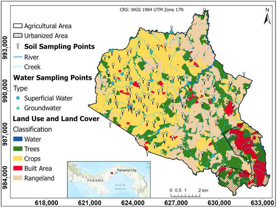
Figure 1.
Study area and sampling sites.
The study area is comprised of two watersheds, the lower part of the Panama Canal watershed and the upper part of the Caimito River watershed. These watersheds are of great importance for the operation of the Panama Canal and for supplying water to the surrounding populations.
The Panama Canal watershed has a great biological diversity influenced by its geological, geographic, and climatic characteristics; the Chagres River is the main river of the watershed; it has a high rainfall, which according to [40] has recently been affected by climatic variations, conditioning the availability of water for the proper functioning of the canal and human supply.
The Caimito River basin has shown a marked human influence, where the most developed sectors are agriculture and livestock; this is a basin that flows into the Pacific, with a topography that ranges from mountainous relief in the upper part to plains in the lower part; the basin shows changes in groundwater in the upper, middle, and lower parts as a result of climate change [41].
This area is characterized by the predominant presence of the Miocene Tucue (TM-CATu) volcanic geological formation. The volcanic rocks in the region are andesitic, basaltic, and tuffaceous in nature. These rocks provide a representative mineralogical content of clay minerals, feldspars, silica, and mafic minerals such as olivine and pyroxene [42]. The mineralogical composition of these rocks directly influences the soil geochemistry and texture of the region through physical and chemical weathering processes that are influenced by environmental factors such as temperature and precipitation [42,43,44].
The hydrogeology of the study area is controlled by the geological units present, mainly basalts and andesites that, when influenced by weathering and fracturing processes, create the necessary conditions of permeability and secondary porosity that allow groundwater storage [45]. Having a variable permeability, these aquifers are restricted to local fracture zones and are considered moderately productive [46]. This hydrogeological context is fundamental to understanding both the availability and quality of groundwater used for agricultural and domestic activities in the study area.
2.2. Sample Collection
Accessible areas within the Herrera township that are used for agricultural activities were considered for soil sampling. This approach made it possible to cover the main production areas of the region, ensuring that the samples adequately represented the edaphic characteristics of the soils used in local agriculture. As for water sampling, priority was given to rivers, streams, and wells used for crop irrigation. Samples were collected during the months of May through July 2024.
Soil samples were taken near the crops, where approximately 1 to 2 kg of soil was sampled using hand augers at a standard depth of 20 cm and stored in airtight plastic bags [47]. Each sample was georeferenced for subsequent spatial analysis, giving a total of 102 soil samples (see Figure 1 and Supplementary Table S1).
A total of 16 water samples were taken, 13 corresponding to surface sources (rivers and streams) used for crop irrigation and 4 well samples to evaluate groundwater conditions and identify a possible relationship between groundwater and agricultural activity (see Supplementary Table S2).
Physicochemical parameters such as pH, EC, salinity, temperature, DO (dissolved oxygen), and TDS were measured in the water samples with a multiparametric field probe (YSI, Professional Plus, Xylem Inc., Brannum Lane Yellow Springs, OH, USA), according to the instructions for in situ sampling of the Standard Methods for Examination of Water and Wastewater, 23rd Edition [48,49,50]. Each water sample was taken in plastic containers for the laboratory analysis of metals (preservative, HNO3 at pH < 2), NO3-N (nitrate) and SO4 (sulfates) (refrigeration, ≤ 6.00 °C), total N (total nitrogen) (preservative, H2SO4 at pH < 2.00), and PO4 (phosphate) (refrigeration, ≤ 6.00 °C).
2.3. Sample Preparation
Soil and water samples were taken to the laboratory of the Faculty of Civil Engineering of the Universidad Tecnológica de Panamá. The soil samples were dried in an oven at 60 °C for 24 h, then were disaggregated with a wooden roller and passed through a 2 mm sieve for further analysis. Twenty grams of the sieved samples was taken to a particle size of 74 μm using an agate roller for X-ray fluorescence metal testing at Laboratorio de Rayos X y Espectroscopía Mössbauer, at the Universidad de Panama. Water samples for sulfate analysis were filtered using 125 mm/diam ash-free filter paper for rapid quantitative analysis. For total N analysis, the pH of the samples was adjusted to 7 with 5 N NaOH solution. For metal analysis, water samples were digested at the Laboratorio de Análisis Industriales y Ciencias Ambientales (LABAICA) del Centro Experimental de Ingeniería of the Universidad Tecnológica de Panamá, where a volume of 3 mL of 65% HNO3 was added to 100 mL of sample, followed by heating in a hotplate to reduce the volume of the solution; the solution obtained was filtered using 125 mm/diam ash-free filter paper for rapid quantitative analysis and adjusted to a final volume of 100 mL with distilled water, which was stored in plastic bottles, ensuring the homogeneity of the sample for analysis.
2.4. Laboratory Analysis
2.4.1. Soil Analysis
Soil samples were taken to the laboratory of the Faculty of Civil Engineering of the Universidad Tecnológica de Panamá. Physicochemical parameters of pH, EC, TDS, and salinity were measured on the sieved samples at a 1:5 (w/v) suspension [51] with an OHAUSS T20M-C multiparameter. Soil texture tests were performed using the Bouyoucos densimeter method [52]. OM was determined by mass loss at 440 °C in a Hobersal HD150 furnace, according to ASTM D2974 [53]. CEC tests were carried out based on the potentiometer method [54].
Out of the 102 total soil samples collected for laboratory analysis, twenty were selected for soluble N (soluble nitrogen) analysis. These selected samples were homogeneously distributed across the study area and analyzed at the Laboratorio de Análisis Industriales y Ciencias Ambientales (LABAICA) of the Centro Experimental de Ingeniería at the Universidad Tecnológica de Panamá, following the persulfate digestion method (HACH 10072) [55], adapted for soil samples.
The sieved samples were sent to Laboratorio de Rayos X y Espectroscopía Mössbauer, at the Universidad de Panamá for the analysis of Al, Ca, Cu (copper), Fe, K, Mg, Mn (manganese), soluble N, P, Si (silicon), Sr (strontium), and Zn content by energy-dispersive X-ray fluorescence spectroscopy (ED-XRF) [4,56,57] with Epsilon4 equipment (Malvern Panalytical, Almelo, the Netherlands), with Omnian software, a pre-calibration routine for all elements based on a calibration curve, and a fundamental parameter (standardless) approach. Certified reference material was used to check both precision and accuracy: NIST 2710A (Montana soil), with recovery percentages between 95.0–100%. In terms of precision, the relative standard deviation (RSD) for all replicates was <10.0%. The limits of detection (LDs) for the different tests were pH = 1.00 × 10⁻², EC = 1.00 × 10⁻³ dS m−1, OM = 1.00 × 10⁻²%, SM = 1.00 × 10⁻²%, CEC = 4.40 × 10⁻¹ cmol kg−1, Al = 1.00 × 10⁻⁴%, Ca = 1.00 mg kg−1, Cu = 1.00 mg kg−1, Fe = 1.00 × 10⁻⁴%, K = 1.00 mg kg−1, Mg= 1.00 mg kg−1, Mn = 1.00 mg kg−1, soluble N = 2.00 mg kg−1, P = 1.00 mg kg−1, Si = 1.00 × 10 −4%, Sr = 1.00 mg kg−1, and Zn = 1.00 mg kg−1. Uncertainties were estimated with a 95.0% confidence interval where k = 2, using the bottom-up approach, described in the Eurachem Guide [58], which consists of identifying and quantifying the sources of uncertainty, and then combining them, where the expanded uncertainties (U exps) are as follows: pH = ±1.00 × 10⁻², EC = ±3.50 × 10⁻⁴ dS m−1, OM = ±1.50 × 10⁻²%, SM = ±1.00 × 10⁻²%, CEC = ±2.10 × 10⁻¹ cmol kg−1, Al = ±1.00 × 10⁻⁵%, Ca = ±1.00 × 10⁻¹ mg kg−1, Cu = ±1.00 × 10⁻¹ mg kg−1, Fe = ±1.00 × 10⁻⁵%, K = ±1.00 × 10⁻¹ mg kg−1, Mg= ±1.00 × 10⁻¹ mg kg−1, Mn = ±1.00 × 10⁻¹ mg kg−1, soluble N = ±2.40 × 10⁻² mg kg−1, P = ±1.00 × 10⁻¹ mg kg−1, Si = ±1.00 × 10⁻⁵%, Sr = ±1.00 × 10⁻¹ mg kg−1, and Zn = ±1.00 × 10⁻¹ mg kg−1. These quality controls ensured the quality of the measured results, making the overall results and conclusions of this study reliable.
2.4.2. Water Analysis
SO4 concentrations in water samples were analyzed following the SulfaVer 4 method (HACH 10248) [59] with certified reference material HC20362013 (Sigma Aldrich, St. Louis, MO, USA). Total N was quantified using the persulfate digestion method (HACH 10208) [60] with certified reference material Cat 15349 (Hach); NO3-N analysis was performed using the cadmium reduction method (HACH 8039) [61] with certified reference material HC17263711 (Sigma Aldrich); PO4 concentrations were determined following the PhosVer 3 Ascorbic Acid method (HACH 8048) [62] with certified reference material HC27970898 (Sigma Aldrich, St. Louis, MO, USA); and HCO3 analysis was performed using the phenolphthalein and total alkalinity method (HACH 8203) [63] with certified reference material 1427810 (Hach, Ames, IA, USA).
The metals Ca, Fe, K, Mg, Mn, and Na were analyzed in the Laboratorio de Análisis Industriales y Ciencias Ambientales (LABAICA) del Centro Experimental de Ingeniería of the Universidad Tecnológica de Panamá by flame atomic absorption spectrometry with AA-7000 equipment (Shimadzu, Kyoto, Japan), using the direct air-acetylene flame method [48] with certified reference material VHG-SM24-100, having a recovery percentages of 90.0–100%. In terms of precision, the relative standard deviation (RSD) for all replicates was <10.0%. The limits of detection (LDs) for the different tests were pH = 1.00 × 10⁻², TDS = 1.00 × 10⁻² mg L−1, DO = 1.00 × 10⁻² mg L−1, Saturation = 1.00 × 10⁻² %, Salinity = 1.00 × 10⁻² mg L−1, NO3-N = 3.00 × 10⁻¹ mg L−1, PO3 = 1.50 mg L−1, HCO3 = 10.0 mg L−1, SO4 = 2.00 mg L−1, total N = 1.00 mg L−1, Ca = 1.08 mg L−1, Fe = 7.10 × 10⁻¹ mg L−1, K = 8.00 × 10⁻² mg L−1, Mg = 1.30 × 10⁻¹ mg L−1, Mn = 5.90 × 10⁻¹ mg L−1, Na = 8.00 × 10⁻² mg L−1. Uncertainties were estimated with a 95% confidence interval where k = 2, using the bottom-up approach, described in the Eurachem Guide [58], which consists of identifying and quantifying the sources of uncertainty and then combining them, where the expanded uncertainties (U exp) are as follows: pH = ±1.00 × 10⁻², TDS = ±1.75 × 10⁻¹ mg L−1, DO = ±2.50 × 10⁻¹ mg L−1, Saturation = ±2.34 %, Salinity = ±2.00 × 10⁻² mg L−1, NO3-N = ±2.40 × 10⁻² mg L−1, PO3 = ±2.80 × 10⁻² mg L−1, HCO3 = ±3.20 × 10⁻¹ mg L−1, SO4 = ±1.36 mg L−1, total N = ±7.60 × 10⁻² mg L−1, Ca = ±5.91 × 10⁻¹ mg L−1, Fe = ±3.84 × 10⁻¹ mg L−1, K = ±1.31 × 10⁻¹ mg L−1, Mg = ±3.85 × 10⁻¹ mg L−1, Mn = ±3.96 × 10⁻¹ mg L−1, Na = ±2.70 × 10⁻¹ mg L−1. These quality controls ensured the quality of the measured results, making the overall results and conclusions of this study reliable.
2.5. Methods
2.5.1. Geo-Accumulation Index (Igeo)
The geo-accumulation index quantifies soil contamination using geochemical background values as a base to assess the content of metals in soil samples [64]. The Igeo is measured using Muller’s Equation (1).
where Cn is the measured content of the metal, Bn is the geochemical background value, and there is a figure of 1.5 for potential fluctuations in background values caused by lithogenic influences. In this study, the geochemical background values (Bns) used were Al = 13.7%, Ca = 2.00 × 10³ mg kg−1, Cu = 1.38 × 10² mg kg−1, Fe = 10.2 %, K = 3.13 × 10² mg kg−1, Mg = 9.55 × 10² mg kg−1, Mn = 2.47 × 10³ mg kg−1, P = 1.03 × 10³ mg kg−1, Si = 19.4 %, Sr = 1.22 × 10² mg kg−1, and Zn = 92.1 mg kg−1. These values correspond to a sample collected from the central region of the study area (code, 06-77; Table S1), characterized by belonging to the proximity of small patches of forest within the township, with low agricultural activity. This limited anthropogenic influence reduces the likelihood of artificial soil enrichment, rendering the sample more representative for evaluating soil contamination.
The Igeo scale, according to Müller [65], is divided into seven grades that indicate the quality of the soils, the definitions for which are listed in Table 1.

Table 1.
Muller’s geo-accumulation index (Igeo) classification [65].
2.5.2. Sodium Adsorption Ratio
The SAR is a critical parameter used to assess the suitability of water for agricultural irrigation, as it helps in understanding the potential impact of soil sodium on the soil structure and crop health [66,67]. The SAR is calculated using the concentrations of Na, Ca, and Mg ions in water. The SAR is calculated according to Equation (2) proposed by Lorenzo A. Richards [68], where the concentrations are in milliequivalents per liter.
2.6. Spatial Interpolation Methods for Soil Nutrient Mapping
Interpolation methods are essential in soil nutrient mapping, enabling the estimation of values at unsampled locations based on spatial patterns. This study selected Kriging and Inverse Distance Weighted (IDW) due to their distinct advantages in modeling soil nutrient distribution. Kriging, a geostatistical method, was chosen for its ability to incorporate spatial autocorrelation, ensuring unbiased predictions with minimal estimation variance. By analyzing semivariograms, Kriging assigns weights based on spatial dependence, allowing for a more accurate representation of nutrient distributions across heterogeneous landscapes [69]. Additionally, Kriging provides an estimation variance metric, which quantifies the reliability of interpolated values, making it a robust choice for applications requiring uncertainty assessment [70]. On the other hand, IDW was selected for its computational efficiency and simplicity, offering a practical alternative for generating soil nutrient maps without the need for complex statistical modeling. Unlike Kriging, IDW directly assigns weights based on inverse distance relationships, making it particularly effective in capturing localized variations in nutrient content, especially in datasets with a strong spatial heterogeneity [71]. Furthermore, IDW does not rely on assumptions of stationarity, making it a flexible approach for irregularly distributed soil samples.
Despite its strengths, Kriging has notable limitations that must be considered. Its accuracy is highly dependent on semivariogram modeling, meaning that an incorrect semivariogram can lead to biased predictions [69]. Additionally, Kriging assumes stationarity, which is often unrealistic in soil science, as nutrient distributions are influenced by factors such as topography, land use, and soil type variations [72]. Another key limitation is its reliance on high-density sampling, as sparse datasets may fail to capture the true spatial correlation, resulting in unreliable interpolations [73,74]. Similarly, IDW has its own constraints, including its tendency to produce over-smoothed surfaces, which can obscure critical spatial trends in soil nutrient variation [71]. Unlike Kriging, IDW does not provide an uncertainty estimation, limiting its applicability in decision-making processes where error quantification is necessary. Furthermore, IDW assumes that the influence of surrounding points decreases uniformly with distance, which may not accurately reflect the complex interactions governing soil nutrient dynamics [21].
Numerous authors, such as Munyati and Sinthumule [75], have discussed the challenge of selecting between Kriging and IDW for spatial interpolation. Their findings suggest that Ordinary Kriging is more suitable for mapping tree density in dense forests, whereas IDW performs better in scattered tree savannah woodlands. Similarly, in this study, IDW was found to be more effective for capturing localized variations in soil nutrients. By integrating both methods, this study leverages Kriging’s ability to provide statistically sound estimations with an uncertainty assessment and IDW’s practicality in handling spatial heterogeneity. This combined approach enhances the reliability of soil nutrient assessments, supporting more informed agricultural decision-making.
2.7. Data Processing
Data wrangling, statistical analysis, principal component analysis (PCA), and visualization were performed using Microsoft 365 Excel (version 2412, Build 16.0.18324.20092) and JupyterLab 4.0.7 with Python 3.10.14. The Riverside diagram for SAR was generated using Diagrammes 8.6. Spatial analysis and map generation were conducted in ArcGIS Pro 3.3.0, utilizing Kriging and Inverse Distance Weighted (IDW) interpolation methods for soil nutrient content mapping. Model validation was ensured by maintaining a Root Mean Square Standardized (RMSS) within the range of 0.8–1.2 and a Root Mean Square Error (RMS) approximating the standard deviations of nutrient content.
3. Results
3.1. Soil Caracterization
3.1.1. Physicochemical Analysis in Soils
Table 2 shows a statistical summary of the content of the physicochemical parameters analyzed in the soil samples from the Herrera township in Panama Oeste; the sample data are presented in Table S1. The mean value pH of the soil is 5.00, being very strongly acid according to the classification of the United States Department of Agricultural National Resources Conservation Service groups [13]. The mean EC is 1.54 × 10⁻¹ dS m−1, corresponding to non-saline soils [12]. The average soil organic matter is 8.43%, which is a high value, indicating that the soil is enriched with organic residues [14]. Humidity is moderate, with a mean value of 27.0% [76]. The area is dominated by a clay type soil (mean value of 65.0%, see soil texture Table 3) with a moderate cation exchange capacity (12.6 cmol kg−1 mean value), which is influenced by the acid pH of the soil [77].
Table 2.
Statistical overview of the content of physicochemical parameters measured in soil samples. Abbreviations: SD, standard deviation.
Table 3.
Texture of soil samples.
The most abundant elements in these soil samples are Si, with a mean value of 22.9 %; Al, with 15.2%; and Fe, with 9.09%. In terms of lower content, we have mean values of Ca>Mg>Mn>P>K (1.58 × 10³ mg kg−1 > 1.57 × 10³ mg kg−1 > 1.38 × 10³ mg kg−1 > 9.99 × 10² mg kg−1 > 6.01 × 10² mg kg−1, respectively). At an even lower content, we have mean values of Cu>Zn>Sr>soluble N (1.25 × 10² mg kg−1 > 8.50 × 101 mg kg−1 > 4.25 × 101 mg kg−1 > 3.08 × 101 mg kg−1, respectively).
Table 4 shows the Panama soil quality standard values, recommended as the maximum permissible for agricultural use, and values from other studies on agricultural soils. The mean value of Zn (85.0 mg kg−1) exceeds that established by the Panamanian standard [78] for agricultural soils and the value of other studies in Chorrera [79] and Colombia [80]. The mean values of this study for OM (8.43 %), Ca (1.58 × 10³ mg kg−1), Cu (1.25 × 10² mg kg−1), Fe (9.09 % mg kg−1), K (6.01 × 10² mg kg−1), Mn (1.38 × 10³ mg kg−1), and P (9.99 × 10² mg kg−1) were higher than those of other agricultural soil studies in La Chorrera [79] and Colombia [80]; and they were lower for CEC (12.6 cmol kg−1), Mg (1.57 × 10³ mg kg−1), and soluble N (30.8 mg kg−1) than Costa Rican soils [81].
Table 4.
Comparison of nutrient standards and reported agricultural soil values.
3.1.2. Spatial Variability in Soils
The study of the spatial variability in the content of elements in the soil through geostatistics, to know the distribution and mapping of their content in the soil, is a very useful tool in agriculture for the management of this natural resource [4]. Comparisons will be made between the maps generated by Kriging and IDW interpolation [12].
Edaphic Parameters
Figure 2 shows the interpolation maps for soil parameters of pH, electrical conductivity, and soil moisture; on the left, the maps were generated using the Kriging method; on the right, using the IDW method. According to the spatial distribution map of soil pH for Kriging and IDW, the northwestern zone of the township of Herrera has a very strong acid pH between 4.50 and 5.09, while the rest of the township has a strong acid pH (5.10 to 5.59); the area with a very strong acid pH is mainly dedicated to intensive pineapple agriculture; the other area corresponds to pastures dedicated to livestock and forest patches, with the exception of the area that is currently urbanized in the southeastern part of the township, where no samples were taken. Soil EC maps in both Kriging and IDW are non-saline (<2.00 dS m−1) throughout the study area; the same trend is found in SM, which is of moderate moisture (20.0–40.0%) throughout the study area.
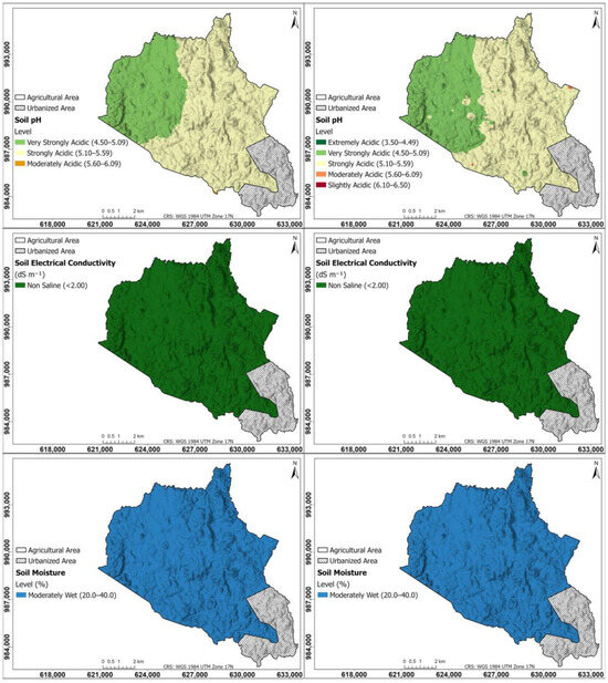
Figure 2.
Interpolation maps for soil parameters of pH, EC, and SM. On the (left), the maps were generated using the Kriging method; on the (right), using the IDW method.
Figure 3 shows the interpolation maps for soil parameters of soil organic matter and cation exchange capacity; on the left, the maps were generated using the Kriging method; on the right, using the IDW method. Soil OM maps in both Kriging and IDW are very high (>6.00%) in the western part of the township, and high (4.00–6.00%) in the rest of the study area. According to the CEC map, the CEC is moderate throughout the entire township, being higher in the northern and eastern parts, between 12.8 and 14.1 cmol kg−1, and in the rest of the study area, between 11.2 and 12.7 cmol kg−1; in the IDW, some points with CEC > 17.3 cmol kg−1 are observed.

Figure 3.
Interpolation maps for soil parameters of OM and CEC. On the (left), the maps were generated using the Kriging method; on the (right), using the IDW method.
Figure 4 shows a soil texture map of the agricultural area generated using the Thiessen polygon method; this map classifies the soil textures present in the region according to the data of the collected samples. According to the texture map, the texture is generally of the clay type in the study area, with certain exceptions, in which clay loam areas stand out in the northern and central part and areas of silty loam and silty clay in the southeastern part.

Figure 4.
Soil texture map of the agricultural area generated using the Thiessen polygon method. This map classifies the soil textures present in the region according to the data of the collected samples.
Primary Nutrients
Figure 5 shows the spatial distribution of the major nutrients for soluble N, P, and K in the agricultural soils of the study area: left maps generated using the Kriging interpolation method; right maps generated using the IDW interpolation method. The soluble N map shows a difference between the Kriging and IDW maps, Kriging shows a central zone with a content between 18.1 and 22.0 mg kg−1 and an external zone between 22.1 and 29.6 mg kg−1; IDW shows the northwestern part with a content higher than 29.6 mg kg−1, and the rest of the zone with a content lower than this, coinciding with the intensive cultivation zone with the highest amounts of soluble N.
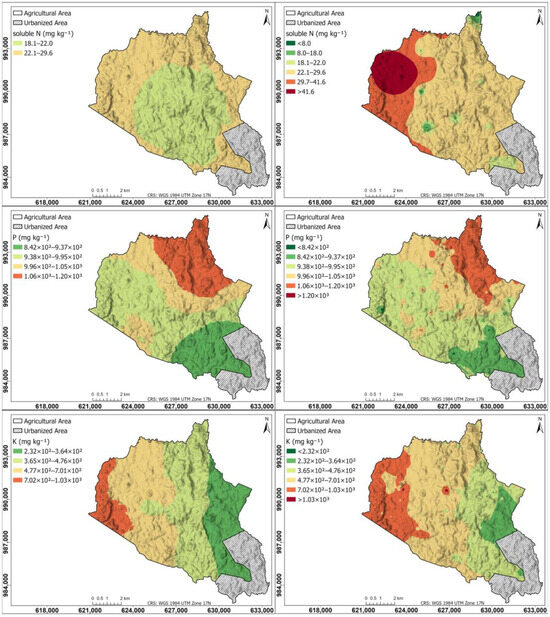
Figure 5.
Spatial distribution of the major nutrients for soluble N, P, and K in the agricultural soils of the study area. (Left) Maps generated using the Kriging interpolation method; (right) maps generated using IDW interpolation method.
The Kriging-generated map for soluble N produced suboptimal results due to the method’s sensitivity to data density. With only 20 sample points, the sparsity of the dataset prevented the semivariogram from accurately capturing the true spatial autocorrelation, leading to less reliable predictions. In contrast, IDW did not require semivariogram modeling, making it less susceptible to errors related to spatial structure estimation. This characteristic allowed IDW to be more robust in interpolating soluble N concentrations, particularly in situations where the spatial dependence structure was unknown. Its robustness stemmed from the stronger weighting of nearby sample points, following the principle that a point’s influence on the prediction decreases with distance. Consequently, IDW provided a more reliable spatial representation of soluble N distribution under the given sampling constraints.
The P map is similar in Kriging and IDW, with higher content in the northern part (>1.05 × 10³ mg kg−1), progressively decreasing towards the south (8.42 × 10² mg kg−1). For the K map in Kriging and IDW, the highest content is in the western part (>7.01 × 10² mg kg−1), progressively decreasing towards the eastern part (2.32 × 10² mg kg−1).
Secondary Nutrients
Figure 6 shows a spatial distribution of secondary nutrients for Ca and Mg in the agricultural soils of the study area: left maps generated using the Kriging interpolation method; right maps generated using the IDW interpolation method. The Ca map is similar in Kriging and IDW, with the highest content in the right half of the township (1.49 × 10²–3.21 × 10³ mg kg−1), an area corresponding mostly to pastures and livestock, and lower content in the western part dedicated to crops (8.31 × 10²–1.48 × 10³ mg kg−1), and within this area there is a region with high values (1.49 × 10³–3.21 × 10³ mg kg−1). The Mg map is similar in Kriging and IDW, with a central strip from north to south with higher content (1.92 × 10³–3.91 × 10³ mg kg−1) and lower values on both sides.
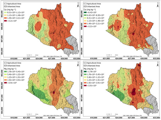
Figure 6.
Spatial distribution of secondary nutrients for Ca and Mg in agricultural soils of the study area. (Left) Maps generated using the Kriging interpolation method; (right) maps generated using the IDW interpolation method.
Micronutrients
Figure 7 shows a spatial distribution of micronutrients for Cu, Fe, Mn, and Zn in the agricultural soils of the study area: left maps generated using the Kriging interpolation method; right maps generated using the IDW interpolation method. The Cu map is similar in Kriging and IDW, with the highest content (1.35 × 10²–1.57 × 10² mg kg−1) in the southern part, decreasing progressively towards the northern part. The high Cu content in the central part of the study area can be attributed to the volcanic geology, characterized by basalts, andesites, and tuffs, which may contain Cu-bearing minerals released through weathering [82,83]. Additionally, the relief and drainage could be promoting Cu accumulation in lower areas due to sediment transport and deposition. Furthermore, agricultural activities, such as the use of Cu-based fungicides, may be contributing to its content in the soil, reinforcing the elevated values observed in the area.

Figure 7.
Spatial distribution of micronutrients for Cu, Fe, Mn, and Zn in the agricultural soils of the study area. (Left) Maps generated using the Kriging interpolation method; (right) maps generated using the IDW interpolation method.
The Fe and Zn maps are similar to each other, and similar in Kriging and IDW, with the highest values in the eastern hemisphere, decreasing progressively towards the western hemisphere. The IDW Mn map shows the southern part with the highest content (1.66 × 10³–2.60 × 10³ mg kg−1), decreasing progressively towards the northwestern part; unlike Kriging, which shows a smaller area of high content in the southern part.
The Mn Kriging map was affected by data non-stationarity, leading to suboptimal predictions due to Kriging’s assumption of a uniform spatial dependence structure. This non-stationarity is attributed to geological and land use factors. The study area consists of volcanic rocks (andesite, basalt, and tuff) rich in Mn-containing minerals, which vary in solubility and reactivity, influencing Mn release into the soil [82,83]. Additionally, redox conditions play a key role in Mn mobility, with reducing environments increasing Mn availability, while oxidizing conditions promote the formation of insoluble Mn oxides, limiting its bioavailability [84,85]. Furthermore, livestock activity contributes to localized Mn enrichment through organic matter deposition and soil acidification, enhancing Mn solubility [86]. Given these strong spatial variations, IDW proved to be more effective.
Other Elements Present in the Soil
Figure 8 shows a spatial distribution of other elements like Si and Sr in the agricultural soils of the study area: left maps generated using the Kriging interpolation method, right maps generated using the IDW interpolation method. The Si map is similar in Kriging and IDW, with the highest content in the western part (25.2–28.0%), decreasing progressively towards the east (17.2–20.9%); the Sr map in Kriging and IDW has a higher content in the northeastern part (46.3–98.7 mg kg−1), decreasing towards the southwestern part (19.1 mg kg−1).
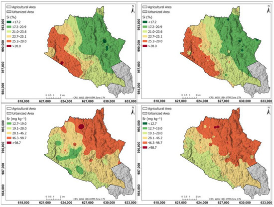
Figure 8.
Spatial distribution of other elements like Si and Sr in the agricultural soils of the study area. (Left) Maps generated using the Kriging interpolation method; (right) maps generated using the IDW interpolation method.
3.1.3. Multi-Element Analysis in Soils
Figure 9 shows a PCA plot of the relationships of the edaphic parameters and soil nutrients. According to the table of the strength of the relationships (Table 5), the most significant relationships are as follows: PC1 explains most of the variability in the data with a 28.4% contribution, followed by PC2 with 14.9% and PC3 with 11.7%. PC1 explains variations in OM (0.350), Fe (0.355), Mg (0.278), and Zn (0.261), which are predominant in the soils of the eastern area of the township that is in pasture for livestock and the forest patch; this explains that in this area that is in rest, and where there are contributions by organic matter from livestock, there is less demand for these nutrients; in this same factor, there is a negative contribution of Al (−0.431) and Si (−0.340), which are predominant in the more acid soils of the northwestern part of the township dedicated to intensive pineapple cultivation.

Figure 9.
PCA of relationship between edaphic parameters and soil nutrients.
Table 5.
PCA matrix for relationship between edaphic parameters and soil nutrients. Bold numbers correspond to PC1 or PC2 or PC3 and are more significant.
PC2 is dominated by Ca (0.454) and K (0.520), which indicates the influence of the fertilization of agricultural soils with these nutrients on this component. And PC3, with main contributions from SM (0.376), pH (0.236), Mg (0.377), and Cu (0.294), indicates the relationship of these edaphic parameters (SM, pH) with the availability of these nutrients.
The PCA graph shows clusters, corroborating that in the group of soils dedicated to intensive pineapple cultivation the presence of Al predominates, which makes these soils the most acidic in the township, while in the soils that are kept in pasture the presence of Ca, Fe, Mg, and Zn predominates, due to the lower demand for these nutrients.
3.1.4. Geo-Accumulation Index
The Igeo has been used to observe which elements may be influenced by anthropogenic activities and which are found in natural content. Figure 10 shows the box plot for the elements of this study. The elements that are naturally occurring, since they had an Igeo < 0, are P, Ca, Mn, Fe, Cu, Zn, Al, Si, and Sr; some of them had certain outliers above zero, such as Ca, Mn, Zn, and Si. The elements that have an Igeo < 1, and where some fraction of their presence may be linked to anthropogenic activities such as agricultural amendments, are K and Mg and some anomalous values of Ca and Zn.

Figure 10.
Box plot of the Igeo values for the elements analyzed in soil samples. Black lines indicate sediment quality categories: <0 uncontaminated, <1 uncontaminated to moderately contaminated, <2 moderately contaminated.
3.2. Irrigation Water Quality
3.2.1. Physicochemical Analysis in Water
Table 6 shows the summary statistics of physicochemical parameter concentrations measured in surface water and groundwater; the sample data are presented in Table S2. The pH has a mean of 6.49 in surface water, which helps to reduce carbonate concentrations and prevents the gradual increase of pH in the soil [87]; groundwater has a mean pH of 7.26, which optimizes the absorption of nutrients in crops, optimizing the solubility of essential nutrients. The mean EC in surface and groundwater is 7.00 × 10⁻² dS m−1 and 2.40 × 10⁻¹ mg L−1, respectively, being low enough to promote crop growth and health [88]. In surface water, the mean TDS is 44.8 mg L−1, and in groundwater there is a considerably higher mean TDS of 1.43 × 10² mg L−1; both mean levels are below 5.00 × 10² mg L−1, which is not considered a risk to crop health [89]. For DO, the mean of surface water and groundwater was 3.57 mg L−1 and 4.17 mg L−1 respectively; for the water body to be considered healthy the DO should be at least 6.50 mg L−1 [90]. Surface water had a mean saturation percentage of 44.6%, while groundwater had a mean of 53.9%; these percentages indicate the presence of clay soils [91]. For salinity, the mean levels of surface water and groundwater were 4.00 × 10⁻² mg L−1 and 1.10 × 10⁻¹ mg L−1, respectively; these values are significantly below 4.50 × 10² mg L−1, which indicates an excellent quality for agricultural use [92].
Table 6.
Statistical overview of the concentrations of physicochemical parameters measured in water samples.
The mean NO3-N levels for surface water were 4.00 × 10⁻² mg L−1 and for groundwater 1.10 × 10⁻¹ mg L−1; both levels are considered low, indicating no significant risk for agricultural growth [93]. PO4 had concentration levels of 1.30 × 10⁻¹ mg L−1 in surface water and 3.60 × 10⁻¹ mg L−1 in groundwater, concentrations considered insufficient to cover the PO4 needs of crops [94]. HCO3 had mean values of 18.0 mg L−1 for surface water and 1.05 × 10² mg L−1 for groundwater; the ideal range of HCO3 in risk waters is 60.0–1.00 × 10² mg L−1 [95]; concentrations below the range can cause instability in the pH of the water, and concentrations above the range greatly increase the pH, causing the removal of vital nutrients. The mean SO4 concentrations were 2.83 mg L−1 and 2.00 mg L−1 in surface water and groundwater, respectively; these concentrations are within the desirable range [96]. Total N had concentrations of 3.92 mg L−1 and 3.00 mg L−1 in surface water and groundwater, respectively; these concentrations are within the acceptable range, without affecting crops [97].
The most abundant elements in surface water were Na (8.27 mg L−1), Mg (3.25 mg L−1), Fe (3.03 mg L−1), Ca (2.05 mg L−1), and K (1.56 mg L−1). For groundwater, the elements with the most abundant means were Na (42.3 mg L−1), Ca (5.13 mg L−1), Mg (4.17 mg L−1), and K (1.87 mg L−1).
Table 7 shows the guideline values of the irrigation water standard in Panama for reused water [98] and international standards for irrigation water from The Texas A&M University [99], University of Massachusetts Amherst [100], and Food and Agriculture Organization of the United Nations (FAO) [101].
Table 7.
Comparison of irrigation water quality standards.
The pH of the surface and groundwater samples comply with the range recommended by the FAO [101]; however, some of the samples are slightly above the limit of 7.00 established by the University of Massachusetts Amherst [100], with values of 7.26 in surface water and 8.80 in groundwater.
As for EC, all the samples presented values significantly below the limits mentioned in the Panama [98] and FAO [101] standards. The maximum TDS measured in surface and groundwater samples was 119 mg L−1 and 321 mg L−1, respectively; both values comply with the standard established by the University of Massachusetts Amherst [100].
The NO3-N concentrations comply with the standards established by the regulations of the University of Massachusetts Amherst [100] and FAO [101], with limits of 5.00 mg L−1 and 15.0 mg L−1, respectively, with the highest concentration of 3.20 mg L−1 belonging to surface water.
The SO4 concentrations for surface and groundwater are considerably below the limit of 3.50 × 10⁵ mg L−1 of the Panama standard [98] and 500 mg L−1 according to FAO [101].
The maximum Ca concentrations for surface water were 4.49 mg L−1 and 10.0 mg L−1 in groundwater, both below the range established by the University of Massachusetts Amherst [100] (40.0 to 100 mg L−1).
For Fe concentrations, the groundwater meets all standards. Surface water complies with the Panama standard [98]; however, it presents concentrations above the limit of 5.00 mg L−1 established by the Texas A&M University [99], University of Massachusetts Amherst [100], and FAO [101] with a maximum concentration of 6.83 mg L−1.
Regarding Mg, none of the samples complies with the minimum limit of 25.0 mg L−1 established by the University of Massachusetts Amherst [100], since all of them present lower concentrations.
For Na, the concentrations in surface water and groundwater comply with Panama’s standards [98]. However, for the University of Massachusetts Amherst standard [100], which establishes a limit of 50.0 mg L−1, only surface water meets this threshold, while groundwater has maximum concentrations of 149 mg L−1.
3.2.2. Sodium Adsorption Ratio (SAR)
The Riverside diagram in Figure 11 uses Wilcox classification [102] to identify the quality of irrigation water considering the SAR and EC of the samples, which are divided into surface and groundwater.
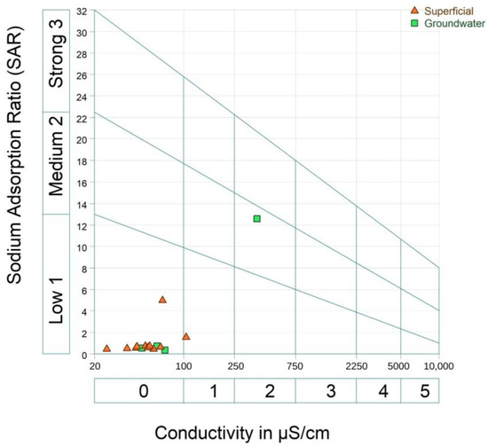
Figure 11.
Riverside diagram of irrigation water classification according to sodium and salinity risks for crops.
It is observed that most of the samples are below class 1, considered to have a low salinity risk, indicating that the water can be used for irrigation without salinization problems; equally, these samples have a low alkalinization level, indicating little danger of developing harmful levels of exchangeable sodium.
Surface water sample 06-70 (see Supplemental Table S2) is in class 1, indicating low salinization and alkalinization, being a safe irrigation source for crops and soils.
Groundwater sample 06-10C (see Supplementary Table S2) is in class 2, presenting a medium salinization and alkalinization risk, not suitable for crops with a low salinization tolerance and fine-textured soils with a high CEC.
3.2.3. Spatial Variability in Water
The spatial distribution of element concentrations in irrigation water is influenced by anthropogenic actions such as agricultural practice and the prolonged use of fertilizers [103]. Irrigation water facilitates the infiltration of metals from surface water to groundwater by rainfall and runoff, resulting in similar concentration patterns in both water sources [104].
Figure 12 shows spatial distribution maps of Ca, Fe, K, Mg, Mn, and Na concentrations in surface water and groundwater.
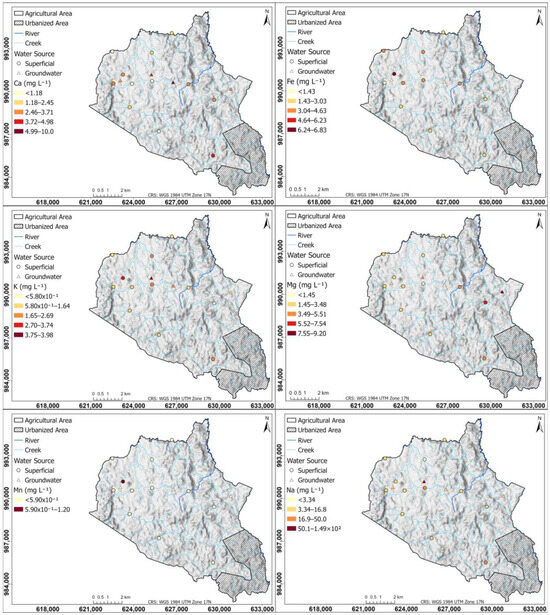
Figure 12.
Spatial distribution of Ca, Fe, K, Mg, Mn, and Na concentrations in surface and groundwater of the study area.
The Ca map presents a heterogeneous distribution in the study area. The maximum values of Ca (10.0 mg L−1), which predominates in groundwater, are located to the northwest, while the lowest concentrations (1.18 mg L−1) are distributed in the western region. To the south, a surface water sample shows higher than average concentrations of 4.98 mg L−1, likely due to domestic wastewater influence. This is attributed to the high level of urbanization in the southern part of the township, where an adequate wastewater treatment system is lacking.
Fe concentrations are high in surface waters due to the low velocity of the water bodies, which causes them to have a low DO, so that under these conditions Fe is converted to soluble forms [105]. The highest value of Fe (6.83 mg L−1 Fe) was found in a water body with very low flow. In groundwater, Fe concentrations are low (<1.43 mg L−1 Fe).
The K map shows a clear high concentration (>1.64 mg L−1) in the northwest of the study area as a sign of strong agricultural activity; these high concentrations are present in surface and groundwater sources, suggesting an interaction of agricultural activities with surface water bodies and K infiltration into aquifers. The lowest concentrations (5.80 × 10⁻¹ mg L−1) are distributed at the limits of the region where agricultural activity is beginning to cease. Concentrations of 2.69 mg L−1 higher than average are found in the south, where surface water is influenced by domestic wastewater activity.
High concentrations (>5.51 mg L−1) in the Mg map are observed in the southeast of the study region, which corresponds to a zone of livestock and crops activity; medium Mg concentrations (3.48 mg L−1) are present in the west of the study area in zones of intense agricultural activity. Concentrations of 5.51 mg L−1 higher than average are observed in the south, where surface water is influenced by domestic wastewater activity.
Mn in surface and groundwater was not detected, except in the water body (1.15 mg L−1 Mn) with low velocity and a low DO in the crop zone, whose anoxic condition allowed solubilization. In the map, the maximum concentrations (1.49 × 10² mg L−1) of Na are found in the middle region in both surface and groundwater sources, which indicates that the activities that take place in this region contribute to Na concentrations in nearby surface water bodies and that soil conditions allow infiltration into aquifers. This maximum concentration is also found in the southern part of the territory, where surface water is influenced by domestic wastewater activity.
3.2.4. Multi-Element Analysis in Water
Figure 13 shows a PCA of relationships between physicochemical parameters for surface and groundwater irrigation. According to Table 8 of relationship strengths, the most significant relationships are as follows: PC1 explains most of the variability in the data with a 41.0% contribution, and on the other hand, PC2 and PC3 explain 21.5% and 12.5%, respectively. With respect to PC1, this component could be related to natural sources by the dissolution of minerals from rocks and by the contributions of pH (0.418) and EC (0.428), related to the concentrations of HCO3 (0.409) and Na (0.370) present in groundwater, especially the well located in the central part of the township, which has the highest values of Na and HCO3. With respect to PC2, it seems to be related to agricultural activities of crops and livestock due to its contribution of DO (0.402), which favors the presence of PO4 (0.337) and Mg (0.427), which are incorporated with synthetic nutrient applications. Finally, PC3 seems to be related to sources of domestic wastewater and agricultural activities contamination by the contribution of NO3-N (0.460) and K (0.389), while Fe contributions (0.357) present in the hematite of the reddish soils of the tropical climate zone [106,107] are dissolved in water bodies with a low DO (−0.384).
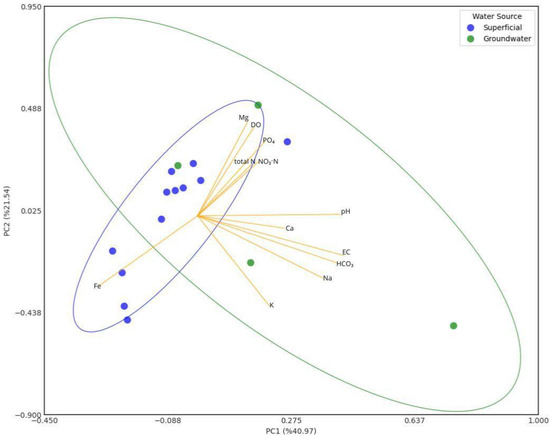
Figure 13.
PCA of relationships between physicochemical parameters for surface and groundwater irrigation.
Table 8.
Principal component analysis matrix for the relationship between physicochemical parameters for surface and groundwater irrigation. Bold numbers correspond to PC1 or PC2 or PC3 and are more significant.
The PCA diagram shows that surface water samples are mostly grouped in the western hemisphere: one group is in the lower left quadrant, where its Fe concentration and low DO concentration prevail; and another group is in the upper left quadrant. Groundwater samples are scattered, not following a trend, which evidences the difference in chemical composition between them.
From the principal component analysis, we observed that DO is a very important parameter in irrigation water, since it conditions the availability of major nutrients such as N and P, which is a very important consideration when selecting water for crop applications. While high EC concentrations are associated with high amounts of Na, this parameter should also be monitored, since Na can salinize soils and is not advisable for crops with a low salinization tolerance.
4. Discussion
4.1. Occurrence of Nutrients in Soil and Water According to Land Use
Regarding the occurrence of nutrients in the soil, the northwestern part of the township of Herrera in Panama Oeste, which is dedicated to pineapple-planting activity in greater intensity, was found to have the most acid pH and the highest content of OM, Si, N, and K; this can be explained by the application of fertilizer amendments with N and K [108] and the application of organic amendments, as well as the decomposition of residual plant material from the crops [109,110].
In the eastern hemisphere of the township, where there are mostly rangelands dedicated to livestock and patches of forests, a higher content of Ca, Fe, Mg, Sr and Zn was found, which could be explained by the fact that this area has a lower demand for nutrients and that the land use rests on pasture and forests [111,112].
In the northern part of the township, we found the highest amounts of P and in the southern part the highest amounts of Cu and Mn; it is possible that these are geochemical anomalies of the area, since these correspond to areas of rangelands and forest patches [113]. Mn is specific to the geology of the site where mafic volcanic rocks, rich in pyroxenes and olivine, can decompose and release Mn in soil-available forms [114]. Similarly, Cu can be derived from the alteration of accessory minerals present in volcanic rocks, such as Cu sulfides or secondary minerals formed during weathering processes [115]. Therefore, the high content of Cu and Mn in the soils of the region may be related to the mineralogical composition of the parent volcanic rocks and their subsequent transformation by geological and edaphic alteration processes.
Soil properties such as EC, CEC, moisture, and texture were homogeneous throughout the study area, giving us an idea of the aptitudes of the area, which in general can be used for agricultural work. Because the soil moisture is good, it is a non-saline soil, with a clayey texture and moderate CEC, which is conducive to agricultural activities [116].
Regarding the water used for irrigation in the northwestern part of the township dedicated to the most intense agricultural activity, K and Na are generally found in higher concentrations in both surface and groundwater, indicating that part of these may come from anthropogenic activities such as agriculture and the application of amendments [117]. In this same area, Fe and Mn were found in higher concentrations in surface water, which may be associated with their oxidation and dissolution on the surface, since the water has a slightly acid pH and less oxygen [118]. Ca was higher in the groundwater of the area, indicating that its presence is linked to the dissolution of material from the rocks of this aquifer [119].
For groundwater and surface water, Mg was found to have the highest concentration in the eastern part of the township; it is possible that this comes from the dissolution of the rocks of the site. The surface water sample taken in the southern part of the township near the urbanized area showed high values of Na and Ca and average values of K, Mg, and Mn, even higher or equal to the most active agricultural zone, which indicates the tainting of these waters with domestic wastewater [120] and prompts the warning that this source should not be used for irrigation or agricultural applications [100].
Although the waters are generally suitable for irrigation according to the standards [87,88,89,90], around the greatest agricultural activity certain points exceed the value of Fe (5.00 mg L−1) and Mn (2.00 × 10⁻¹ mg L−1), again linked to the slightly acidic pH of the waters and low oxygenation. The groundwater in the central zone exceeds the Na value (50.0 mg L−1) according to the University of Massachusetts standard [100], thus presenting a medium salinization and alkalinization risk for crops. This presence of Na is due to the solubilization of the rocks at this depth (52.0 m). This source is not regularly used for irrigation due to the rainfall in the area, and its use is considered only in cases where the dry season is longer than usual.
In general terms, relating water quality and its influence on the soil and crops, we can say that the data provided do not lead us to think that water can salinize the soil, since waters with values lower than 7.00 × 10⁻¹ dS m−1 are considered non-saline [121], and in this study this value is not reached, so the use of these waters has no risk of salinizing the soil or affecting crop growth.
4.2. Evaluation of Soil Suitability for Pineapple Cultivation
Our study area has clay soils (mean value 65.0% clay) of an oxisols type typical of tropical climates; these are acid soils with H+ and Al, Ca, Mg, and K content, which, although they are of low fertility for other types of crops (needing limestone amendments to adjust the pH and fertilizers to be productive), are recommended soils for pineapple cultivation [122]. The pineapple crop adapts well to acid soils with a pH between 4.50 and 5.50 [122], and with average pH values of 5.00 in our study area making it suitable for this crop. The pineapple plant is tolerant to soils with an acid pH, since it tolerates the exchange of Al and Mg that acidifies the soil [122,123].
It favors well-drained and aerated soils to reduce the risk of the pathogenic fungus Phytophthora, and it is recommended that slopes do not exceed 5% to facilitate mechanical tillage and avoid soil loss due to erosion [122]. Most of the areas dedicated to intensive pineapple cultivation have these conditions.
Regarding the requirements of the primary and secondary nutrients that the soil must have to support the pineapple crop, the optimum soluble N is 27.0 mg kg−1; P > 20.0 mg kg−1; the optimum K is 150 mg kg−1; Ca > 100 mg kg−1; and the optimum Mg is 50.0 mg kg−1 [124]. For the Herrera township, we have an average soluble N of 30.8 mg kg−1 and minimum of 2.00 mg kg−1, so depending on the site and its content it will be necessary to apply N amendments; for P, the mean value is 999 mg kg−1 and the minimum 554 mg kg−1, so in all the corregimiento the recommended value is met; for K, the mean value is 999 mg kg−1 and the minimum 133 mg kg−1, which, according to the maps generated, in almost all of the township complies with the optimum value (150 mg kg−1); for Ca, the minimum value is 446 mg kg−1, and the whole township complies with the recommended value; and for Mg, the mean value is 1.57 × 10³ mg kg−1, and the minimum is 53.7 mg kg−1 in some small areas, which means that the township complies with the optimum value. According to this evaluation, N amendments would be mostly required, and the monitoring of those nutrients whose content is close to the optimum would be necessary to know the right moment to make the amendment with the necessary nutrient.
The micronutrients Cu, Fe, Mn, and Zn are required to a lesser extent and are easily absorbed at an acid pH [124], such as is the pH of the soil of the Herrera township (a mean pH of 5.00). A deficiency in these nutrients can occur if the soil pH becomes higher than 6.00 [124]. Therefore, under current conditions no amendments of these micronutrients are required.
As for the evaluation of nutrients (Ca, Fe, K, Mg, Mn, NO3) in the water for irrigation, in general it is suitable according to the evaluated standards [87,88,89,90] in the entire corregimiento.
Regarding the use of groundwater for irrigation, which is an option for use during the dry season, it is not advisable to use the well in the central zone of the township (06-10C) as a source due to its high EC and Na concentrations, which represents a medium risk of the salinization and alkalinization of the soil, which would affect crops with a low tolerance to salinization [91].
4.3. Implications for Sustainable Natural Resource Management and Public Policy
The study of soil and irrigation water quality and its representation through nutrient maps is a very useful tool for the producer, since it will allow him to make intelligent amendments that in turn will allow him to maximize his economic benefits and reduce the impact on the environment [125]. Thus, this research seeks to innovate and contribute to the sustainable management of soil and water resources in the township of Herrera, which is known to produce export-quality pineapple, so that with this contribution farmers can implement the application of intelligent amendments and not ones based only on their traditional knowledge.
For the sustainable management of agricultural soils, practices such as soil health improvement, water management, and a reduction in pesticide use must be implemented [126], contributing to climate change adaptation.
As for the management, maintenance, and improvement of soil health, it is a topic for extensive research that needs to be implemented in the township of Herrera, since the agricultural zone is currently dedicated mainly to pineapple cultivation and the pasture zone to cattle raising. Practices such as reducing tillage, crop rotation, intercropping, polyculture, cover crops, and mulching [126] could be implemented, as these practices have been shown to increase crop yields by improving soil water retention, especially in times of drought; this also reduces soil erosion and thus the loss of nutrients through runoff during the rainy season.
Water management is very important; although Panama is a tropical country with abundant rainfall, it is necessary to make appropriate use of the resource in the dry season and when climatic phenomena such as El Niño occur, in which drought is widespread, causing great concern for farmers [127]. In these cases, measures such as smart irrigation and water harvesting can be implemented as measures against climate change [128].
Producers need to be accompanied by the State in the process of the sustainable management of the natural resources, water and soil, even more so in current climate change scenarios. Among Panama’s public policies is Law 352 of 2023, which establishes the State Agrifood Policy [91]; Article 72, paragraph 5 speaks of ensuring the sustainability and rational use of natural resources, water, soil, and biotic resources in general, within the framework of efforts to increase the productivity and competitiveness of the agrifood sector and its resilience to climate change.
5. Conclusions
This study has been developed to contribute to the sustainable management of the natural resources, water and soil, in the agricultural township of Herrera, Panama Oeste, as a support tool for small and medium farmers. In this context, maps of nutrients in soil and nutrient concentrations in water used for irrigation have been generated. This study is the first to characterize the soil resource of a complete agricultural township in Panama.
In general, the water resource complies with the standards for irrigation water in relation to the nutrients Ca, Fe, Mg, and Mn evaluated. As for Na, it complies with the irrigation water standards of the University of Massachusetts, except in the central agricultural area, where groundwater can be influenced by rock salts; so this source must be used with care, since it represents a risk of salinization and medium alkalinity for the soil and can affect crops with a low tolerance to salinity.
In terms of edaphic properties, the soil is non-saline, with moderate humidity, a high OM content, and moderate CEC, which gives it good properties for agricultural activity.
Depending on the crop to be grown, pH amendments would be required, since the soil is very acidic (a mean value pH of 5.00) in the area dedicated to crops; also, with respect to the other nutrients, depending on the crop, intelligent amendments could be made, taking the nutrient maps of this research as a reference line.
As for the evaluation of the soil and its suitability for pineapple cultivation, it is a well-drained clayey soil, with an average acid pH of 5.00, and it meets the required levels of P, K, Ca, Mg, Fe, Zn, Mn, and Cu. It does require N amendments, for which the soluble N map is a guide to make intelligent amendments of this primary nutrient, which is essential for good crop development.
Supplementary Materials
The following supporting information can be downloaded at: https://www.mdpi.com/article/10.3390/agriculture15070702/s1, Table S1: Assay data measured on soil samples for Herrera, Panama Oeste; and Table S2: Assay data measured in water samples for Herrera, Panama Oeste.
Author Contributions
Conceptualization, A.C.G.-V.; methodology, A.C.G.-V., F.J.G.-N., J.O., J.L., J.A. and F.V.; software, A.C.G.-V., J.A. and T.C.; validation, A.C.G.-V.; formal analysis, A.C.G.-V., T.C., J.O., J.L., J.A., M.D. and J.J.; investigation, A.C.G.-V. and T.C.; resources, A.C.G.-V.; data curation, A.C.G.-V.; writing—original draft preparation, A.C.G.-V., T.C., J.O., J.L., J.A., S.J.-O. and F.V.; writing—review and editing, A.C.G.-V., S.J.-O. and F.J.G.-N.; visualization, A.C.G.-V. and S.J.-O. supervision, A.C.G.-V., S.J.-O. and F.J.G.-N.; project administration, A.C.G.-V.; funding acquisition, A.C.G.-V. All authors have read and agreed to the published version of the manuscript.
Funding
This research was funded by the Secretaría Nacional de Ciencia, Tecnología e Innovación (SENACYT) of Panama, Project FIED23-06, Nutrient geochemical map for the agricultural zone of Herrera, Panama Oeste, grant number ID No. 139-2023; and the Sistema Nacional de Investigación (SNI) de Panama, SENACYT, grant number SNI economic incentive contract No. 010-2023.
Institutional Review Board Statement
Not applicable.
Data Availability Statement
Laboratory analysis data generated in this study are available in the supplemental tables in https://www.mdpi.com/article/10.3390/agriculture15070702/s1, Table S1: Assay data measured on soil samples for Herrera, Panama Oeste; and Table S2: Assay data measured in water samples for Herrera, Panama Oeste.
Acknowledgments
We thank the Universidad Tecnológica de Panamá (UTP) for their research support and the Centro de Estudios Multidisciplinarios en Ciencias, Ingeniería y Tecnología (CEMCIT AIP) for administering the project funds. We thank the Ministry of Agricultural Development Region 5, Panama Oeste, and the Honorable Representante of the township for liaising with the community, and the farmers of Herrera for giving us access to their farms to conduct this study.
Conflicts of Interest
The authors declare no conflicts of interest.
References
- ONU Sustainable Development Goals. Available online: https://www.undp.org/es/sustainable-development-goals (accessed on 1 February 2025).
- Castillo, E.; Delgado, O.; León, H.D.; Escartin, L.; Saéz, Y.; Collado, E. Mejoramiento del uso de suelo en la agricultura mediante herramientas basadas en optimización. I+D Tecnológico 2021, 17, 41–48. [Google Scholar] [CrossRef]
- Agarwal, J.; Vaswani, S.; Sharma, A.; Kaushik, D.; Bhardwaj, D. Optimization of Crop Yield Using Machine Learning. In Proceedings of the 2023 3rd International Conference on Technological Advancements in Computational Sciences (ICTACS), Tashkent, Uzbekistan, 1–3 November 2023; pp. 469–474. [Google Scholar]
- Jiménez-Ballesta, R.; García-Navarro, F.J.; Amorós, J.A.; Pérez-de-los-Reyes, C.; Bravo, S. On the Scarce Occurrence of Arsenic in Vineyard Soils of Castilla La Mancha: Between the Null Tolerance of Vine Plants and Clean Vineyards. Pollutants 2023, 3, 351–359. [Google Scholar] [CrossRef]
- Nursapina, K.U.; Uryngaliyeva, A.; Kuangaliyeva, T.K.; Balkibayeva, A. Factors Influencing Agricultural Innovations. J. Econ. Res. Bus. Adm. 2023, 146, 126–134. [Google Scholar] [CrossRef]
- Miller-Klugesherz, J.A.; Sanderson, M.R. Good for the Soil, but Good for the Farmer? Addiction and Recovery in Transitions to Regenerative Agriculture. J. Rural Stud. 2023, 103, 103123. [Google Scholar] [CrossRef]
- El Alem, A.; Hmaissia, A.; Chokmani, K.; Cambouris, A.N. Quantitative Study of the Effect of Water Content on Soil Texture Parameters and Organic Matter Using Proximal Visible—Near Infrared Spectroscopy. Remote Sens. 2022, 14, 3510. [Google Scholar] [CrossRef]
- Liuzza, L.M.; Bush, E.W.; Tubana, B.S.; Gaston, L.A. Determining Nutrient Recommendations for Agricultural Crops Based on Soil and Plant Tissue Analyses Between Different Analytical Laboratories. Commun. Soil Sci. Plant Anal. 2020, 51, 392–402. [Google Scholar] [CrossRef]
- Prem Kumar, S.; Sahifa, S.; Saadhana, B.N.; Sai Sahithi, M.; Pranathi Ketura, D. Crop Selection and Yield Prediction Using Intelligent Algorithms. In Proceedings of the 2024 International Conference on Expert Clouds and Applications (ICOECA), Bengaluru, India, 18–19 April 2024; pp. 420–425. [Google Scholar]
- Vargas, B. Propiedades Químicas del Suelo en Cuatro Fincas de la Agricultura Suburbana en Santiago de Cuba. Available online: https://www.researchgate.net/publication/350451816_Propiedades_quimicas_del_suelo_en_cuatro_fincas_de_la_agricultura_suburbana_en_Santiago_de_Cuba (accessed on 22 January 2025).
- Mustafa, A.R.A.; Abdelsamie, E.A.; Mohamed, E.S.; Rebouh, N.Y.; Shokr, M.S. Modeling of Soil Cation Exchange Capacity Based on Chemometrics, Various Spectral Transformations, and Multivariate Approaches in Some Soils of Arid Zones. Sustainability 2024, 16, 7002. [Google Scholar] [CrossRef]
- Benslama, A.; Khanchoul, K.; Benbrahim, F.; Boubehziz, S.; Chikhi, F.; Navarro-Pedreño, J. Monitoring the Variations of Soil Salinity in a Palm Grove in Southern Algeria. Sustainability 2020, 12, 6117. [Google Scholar] [CrossRef]
- Oshunsanya, S.O. Introductory Chapter: Relevance of Soil pH to Agriculture. In Soil pH for Nutrient Availability and Crop Performance; IntechOpen: London, UK, 2018; ISBN 978-1-78985-016-1. [Google Scholar]
- Riches, D.; Porter, I.J.; Oliver, D.P.; Bramley, R.G.V.; Rawnsley, B.; Edwards, J.; White, R.E. Review: Soil Biological Properties as Indicators of Soil Quality in Australian Viticulture. Aust. J. Grape Wine Res. 2013, 19, 311–323. [Google Scholar] [CrossRef]
- Mamatha, B.; Mudigiri, C.; Ramesh, G.; Saidulu, P.; Meenakshi, N.; Prasanna, C.L. Enhancing Soil Health and Fertility Management for Sustainable Agriculture: A Review. Asian J. Soil Sci. Plant Nutr. 2024, 10, 182–190. [Google Scholar] [CrossRef]
- Preshanth, V.P.; Parida, V.; Sharma, V.; Verma, Y.; Saini, Y. IOT Based Soil pH Level Maintaining System. Int. J. Sci. Eng. Dev. Res. 2022, 7, 110–113. [Google Scholar]
- Ban, B.; Lee, J.; Ryu, D.; Lee, M.; Eom, T.D. Nutrient Solution Management System for Smart Farms and Plant Factory. In Proceedings of the 2020 International Conference on Information and Communication Technology Convergence (ICTC), Jeju Island, Republic of Korea, 20–21 October 2020; pp. 1537–1542. [Google Scholar]
- Kumari, A.; Mishra, P.; Chaulya, S.K.; Prasad, G.M.; Nadeem, M.; Kisku, V.; Kumar, V.; Chowdhury, A. Estimation of Soil Nutrients and Fertilizer Dosage Using Ion-Selective Electrodes for Efficient Soil Management. Commun. Soil Sci. Plant Anal. 2024, 55, 1920–1941. [Google Scholar] [CrossRef]
- Malhi, S.S. Relative Effectiveness of Various Amendments in Improving Yield and Nutrient Uptake under Organic Crop Production. Open J. Soil Sci. 2012, 2, 299–311. [Google Scholar] [CrossRef]
- Sarwade, P.P.; Gaisamudre, K.N.; Gaikwad, R.S. Mycorrhizal Fungi in Sustainable Agriculture: Enhancing Crop Yields and Soil Health. Plantae Sci. 2024, 7, 55–61. [Google Scholar] [CrossRef]
- Singh, V. Advances in Precision Agriculture Technologies for Sustainable Crop Production. J. Sci. Res. Rep. 2024, 30, 61–71. [Google Scholar] [CrossRef]
- Zhang, Q. Precision Agriculture Technology for Crop Farming; CRC Press: Boca Raton, FL, USA, 2015; ISBN 978-0-429-15968-8. [Google Scholar]
- Wen, T.; Luo, Y.; Tang, M.; Chen, X.; Shao, L. Effects of Representative Elementary Volume Size on Three-Dimensional Pore Characteristics for Modified Granite Residual Soil. J. Hydrol. 2024, 643, 132006. [Google Scholar] [CrossRef]
- MICI Consumidores Españoles Eligen Piña Panameña como ‘Sabor del año 2023’. Available online: https://mici.gob.pa/2023/02/28/ (accessed on 6 February 2025).
- González, A.; Montenegro, V.; Hernández, D.; Domínguez, A.; Castañeda, Y.; Adames, R.; Percival, H.; Vergara, A.; Zamora, A.; Vargas, Y.; et al. Estudio geoquímico de pH y conductividad eléctrica en una finca piñera, Zanguenga, La Chorrera. I+D Tecnológico 2023, 19, 56–63. [Google Scholar] [CrossRef]
- Ministerio de Comercio e Industrias Análisis del Desempeño Reciente de las Exportaciones de Piña en Panamá y en el Mundo. Available online: https://intelcom.gob.pa/informe/analisis-del-desempeno-reciente-de-las-exportaciones-de-pina-en-panama-y-en-el-mundo (accessed on 6 February 2025).
- Intagri Requerimientos de Fertilidad de Suelos para el Cultivo de la Piñade la Piña|Intagri, S.C. Available online: https://www.intagri.com/articulos/frutales/requerimientos-de-fertilidad-de-suelo-para-pina (accessed on 6 February 2025).
- Suleymanov, A.; Abakumov, E.; Suleymanov, R.; Gabbasova, I.; Komissarov, M. The Soil Nutrient Digital Mapping for Precision Agriculture Cases in the Trans-Ural Steppe Zone of Russia Using Topographic Attributes. ISPRS Int. J. Geo-Inf. 2021, 10, 243. [Google Scholar] [CrossRef]
- Rhymes, J.; Chadwick, D.R.; Williams, A.P.; Harris, I.M.; Lark, R.M.; Jones, D.L. Evaluating the Accuracy and Usefulness of Commercially-Available Proximal Soil Mapping Services for Grassland Nutrient Management Planning and Soil Health Monitoring. Precis. Agric. 2023, 24, 898–920. [Google Scholar] [CrossRef]
- Wang, Y.; Qi, Q.; Wang, J.; Wang, M.; Ye, Y. The Potential of Image Segmentation Applied to Sampling Design for Improving Farm-Level Multi-Soil Property Mapping Accuracy. Precis. Agric. 2023, 24, 2350–2373. [Google Scholar] [CrossRef]
- Meena, N.K.; Gautam, R.; Tiwari, P.; Sharma, P. Nutrient Losses in Soil Due to Erosion. J. Pharmacogn. Phytochem. 2017, 6, 1009–1011. [Google Scholar]
- Navarro, G.; Navarro, S. Química Agrícola: Química del Suelo y de los Nutrientes Esenciales para las Plantas. Available online: https://www.mundiprensa.com/catalogo/9788484766568/quimica-agricola--quimica-del-suelo-y-de-los-nutrientes-esenciales-para-las-plantas (accessed on 22 January 2025).
- Rilwanu, T.U.Y.; Hassan, F.Y.; Usman, B.; Yalwa, I.R. GEO-Accumulation Index for Heavy Metals in Groundwater: A Study of Bompai and Sharada Industrial Estates, Kano Metropolis, Nigeria. J. Sustain. Nat. Resour. 2022, 3, 58–72. [Google Scholar]
- Esmail, A.O.E.; Rajab, K.S.R. Effect of Chemical Composition of Irrigation Water on Some Growth and Yield of Corn and P-Availability in Calcareous Soil. In Proceedings of the 2nd International Conference of Agricultural Sciences, Dnipro, Ukraine, 16–17 November 2022; pp. 699–706. [Google Scholar] [CrossRef]
- Acharya, G.D.; Solanki, M.R.; Hathi, M.V. Studies on Physico-Chemical Parameters of Irrigation Water, Prantij, Gujarat (India). Int. J. Chem. Sci. 2010, 8, 2377–2385. [Google Scholar]
- Rieu, M. Sodium Adsorption Ratio et estimation du pouvoir alcalinisant des eaux. Cahiers ORSTOM.Série Pédologie 1981, 18, 123–128. [Google Scholar]
- Vafakhah, M.; Janizadeh, S. Chapter 6-Application of Artificial Neural Network and Adaptive Neuro-Fuzzy Inference System in Streamflow Forecasting. In Advances in Streamflow Forecasting; Sharma, P., Machiwal, D., Eds.; Elsevier: Amsterdam, Netherlands, 2021; pp. 171–191. ISBN 978-0-12-820673-7. [Google Scholar]
- Instituto Nacional de Estadística y Censo. Available online: https://www.inec.gob.pa/publicaciones/Default3.aspx?ID_PUBLICACION=1199&ID_CATEGORIA=19&ID_SUBCATEGORIA=71 (accessed on 23 January 2025).
- Dávila-Sánchez, R. Capa de Clasificación Climática Según Dr. A. McKay (2000). 1:50.000. Panamá. Available online: https://www.arcgis.com/home/item.html?id=680dbb7153ff427196550e0646fb0f98 (accessed on 23 January 2025).
- ACP Cuenca Hidrográfica. Available online: https://pancanal.com/cuenca-hidrografica (accessed on 10 October 2024).
- Mosquera Ballejo, C. Soluciones Basadas En La Naturaleza Para Enfrentar los Riesgos Hidrometereológicos en el Sistema Municipal del Distrito de la Chorrera Ubicado en la Cuenca de Río Caimito, Panamá Oeste, Panamá. Master’s Thesis, CATIE, Turrialba, Costa Rica, 2023. [Google Scholar]
- Asniar, N.; Purwana, Y.M.; Surjandari, N.S. Tuff as Rock and Soil: Review of the Literature on Tuff Geotechnical, Chemical and Mineralogical Properties around the World and in Indonesia. AIP Conf. Proc. 2019, 2114, 050022. [Google Scholar] [CrossRef]
- Alexandre, P. Practical Geochemistry; Springer Textbooks in Earth Sciences, Geography and Environment; Springer International Publishing: Cham, Switzerland, 2021; ISBN 978-3-030-72452-8. [Google Scholar]
- Tuncay, T.; Dengiz, O. Chemical Weathering Rates and Geochemical-Mineralogical Characteristics of Soils Developed on Heterogeneous Parent Material and Toposequence. Carpathian J. Earth Environ. Sci. 2016, 11, 583–598. [Google Scholar]
- Jain, P.; Soni, A.; Shende, R. Management of Hard Rock Basaltic Aquifer through Aquifer Mapping: A Case Study of Nashik District, Maharashtra, India; IntechOpen: London, UK, 2023. [Google Scholar] [CrossRef]
- IMHPA. Mapa Hidrogeológico de Panamá-Instituto de Meteorología e Hidrología de Panamá. Available online: https://www.imhpa.gob.pa/es/mapa-hidrogeologicopanama (accessed on 23 January 2025).
- González-Valoys, A.C.; Esbrí, J.M.; Campos, J.A.; Arrocha, J.; García-Noguero, E.M.; Monteza-Destro, T.; Martínez, E.; Jiménez-Ballesta, R.; Gutiérrez, E.; Vargas-Lombardo, M.; et al. Ecological and Health Risk Assessments of an Abandoned Gold Mine (Remance, Panama): Complex Scenarios Need a Combination of Indices. Int. J. Environ. Res. Public Health 2021, 18, 9369. [Google Scholar] [CrossRef]
- Rice, E.W.; Baird, R.B.; Eaton, A.D. Standard Methods for the Examination of Water and Wastewater, 23rd ed.; American Public Health Association; American Water Works Association; Water Environment Federation: Washington, DC, USA, 2017; ISBN 978-0-87553-287-5. [Google Scholar]
- González-Valoys, A.C.; Vargas-Lombardo, M.; Higueras, P.; García-Navarro, F.J.; García-Ordiales, E.; Jiménez-Ballesta, R. Hydrochemistry of Groundwater from Tocumen Sector, Panamá City: An Assessment of Its Possible Usage during Emergency Events. Environ. Earth Sci. 2021, 80, 176. [Google Scholar] [CrossRef]
- Domínguez, A.; Segundo, F.; Arrocha, J.; Miranda, L.; Chong, T.; Sandoval, H.; Martínez, E.; Gutiérrez, E.; Rodríguez, R.; Nieto, C.; et al. Geochemical Insights into Health Risks from Potentially Toxic Elements in Rural Aqueducts of Cocle, Panama: Unveiling Links to Local Geology. Water 2025, 17, 110. [Google Scholar] [CrossRef]
- ASTM D4972-19; Standard Test Methods for pH of Soils. ASTM: West Conshohocken, PA, USA, 2024. [CrossRef]
- Bouyoucos, G.J. Hydrometer Method Improved for Making Particle Size Analyses of Soils. Agron. J. 1962, 54, 464–465. [Google Scholar] [CrossRef]
- ASTM D2974-14; Standard Test Methods for Moisture, Ash, and Organic Matter of Peat and Other Organic Soils. ASTM: West Conshohocken, PA, USA, 2020. Available online: https://www.astm.org/d2974-14.html (accessed on 4 March 2025).
- Jackson, M.L. Análisis Químico de Suelos; Omega: Barcelona, Spain, 1976; ISBN 84-282-0261-3. [Google Scholar]
- Hach Nitrogen (Total), HR (2-150 Mg/L N), Method 10072. Available online: https://www.hach.com/asset-get.download.jsa?id=7639983803&srsltid=AfmBOoqFAv0gj1oj418j74XM-SnPEFHEQzZkMlygiwQ_VX-j8S-_1-pi (accessed on 26 January 2025).
- Bravo, S.; Jiménez-Ballesta, R.; Amorós, J.A.; Pérez-de-los-Reyes, C.; Villena, J.; García-Navarro, F.J. Accumulation, Distribution Pattern and Potential Contamination of Sulphur in Vineyard Soils of the Valdepeñas Protected Denomination Origin. Sci. Total Environ. 2023, 904, 166642. [Google Scholar] [CrossRef] [PubMed]
- Jiménez-Ballesta, R.; Bravo, S.; Amorós, J.A.; Pérez-de-los-Reyes, C.; García-Pradas, J.; Sanchez, M.; García-Navarro, F.J. Occurrence of Some Rare Earth Elements in Vineyard Soils under Semiarid Mediterranean Environment. Environ. Monit. Assess. 2022, 194, 341. [Google Scholar] [CrossRef]
- Ellison, S.; Roesslein, M.; Williams, A.; Berglund, M. Eurachem/CITAC Guide CG4. Quantifying Measurement Uncertainty in Analytical Measurement. Available online: https://www.researchgate.net/publication/236884859_EurachemCITAC_Guide_CG4_Quantifying_Measurement_Uncertainty_in_Analytical_Measurement (accessed on 3 March 2025).
- Hach SulfaVer 4, (2–70 Mg/L SO4), Method 10248. Available online: https://www.hach.com/asset-get.download.jsa?id=9595814106&srsltid=AfmBOooEv3YHC5vrztF5hZdisdLzPWLDfB6fHDSFOOU8WEkLLd6A32cS (accessed on 29 January 2025).
- Hach Nitrogen (Total), LR (1-16 mg\L N), Method 10208. Available online: https://www.hach.com/p-nitrogen-total-tntplus-vial-test-lr-1-16-mgl-n-25-tests/TNT826?srsltid=AfmBOoowhRxc2Arm_qK2b4EF2zqLvLRJfjG7iK67HH6cGdN1gYkaFs11 (accessed on 25 January 2025).
- Hach Nitrate, HR (0.3–30.0 Mg/L NO3), Method 8039. Available online: https://www.hach.com/asset-get.download.jsa?id=7639983736&srsltid=AfmBOorfiJh41g72RgiyLOdTmAzuaJJHLG6N-XGJ1Z-yKAdyYHZ2nd1p (accessed on 27 January 2025).
- Hach Phosphorus (Reactive), (0.02–2.50 Mg/L PO4), Method 8048. Available online: https://coessing.org/wp-content/uploads/2018/08/phosphorus_reactive_ortho_8048.pdf (accessed on 26 January 2025).
- Hach Alkalinity, (10–4000 Mg/L CaCO3), Method 8203. Available online: https://www.hach.com/asset-get.download-en.jsa?id=7639983930&srsltid=AfmBOoqelb8H8d9HtPrRTQRLD4asHdh4793IVKaU_SRGJOReEJLumWex (accessed on 27 January 2025).
- Elemile, O.O.; Gana, A.J.; Ejigboye, P.O.; Ibitogbe, E.M.; Olajide, O.S.; Ibitoye, O.O. Analysis of Potentially Toxic Elements from Selected Mechanical Workshops Using the Geo-Accumulation Index and Principal Component Analysis in Omu-Aran Community, Nigeria. Environ. Monit. Assess. 2023, 195, 276. [Google Scholar] [CrossRef]
- Muller, G. Index of Geoaccumulation in Sediments of the Rhine River. J. Geol. 1979, 2, 108–118. [Google Scholar]
- Jamei, M.; Ali, M.; Karbasi, M.; Karimi, B.; Jahannemaei, N.; Farooque, A.A.; Yaseen, Z.M. Monthly Sodium Adsorption Ratio Forecasting in Rivers Using a Dual Interpretable Glass-Box Complementary Intelligent System: Hybridization of Ensemble TVF-EMD-VMD, Boruta-SHAP, and eXplainable GPR. Expert Syst. Appl. 2024, 237, 121512. [Google Scholar] [CrossRef]
- Permatasari, A.A.; Vienastra, S. Kelayakan Air Tanah Untuk Irigasi Pertanian Menggunakan Sodium Arbsoption Ratio (SAR). COMSERVA J. Penelit. Dan Pengabdi. Masy. 2022, 2, 497–505. [Google Scholar] [CrossRef]
- Richards, L.A. Diagnosis and Improvement of Saline and Alkali Soils; U.S. Department of Agriculture: Washington, DC, USA, 1954. [Google Scholar]
- Burgess, T.M.; Webster, R. Optimal Interpolation and Isarithmic Mapping of Soil Properties. J. Soil Sci. 1980, 31, 315–331. [Google Scholar] [CrossRef]
- Campbell, K. Kriging for Interpolation of Sparse and Irregularly Distributed Geologic Data; Los Alamos National Laboratory (LANL): Los Alamos, NM, USA, 1986. [Google Scholar]
- Qiao, P.; Li, P.; Cheng, Y.; Wei, W.; Yang, S.; Lei, M.; Chen, T. Comparison of Common Spatial Interpolation Methods for Analyzing Pollutant Spatial Distributions at Contaminated Sites. Environ. Geochem. Health 2019, 41, 2709–2730. [Google Scholar] [CrossRef]
- Song, X.-D.; Zhang, G.-L.; Liu, F.; Li, D.-C.; Zhao, Y.-G. Characterization of the Spatial Variability of Soil Available Zinc at Various Sampling Densities Using Grouped Soil Type Information. Environ. Monit. Assess. 2016, 188, 600. [Google Scholar] [CrossRef]
- Dash, P.K.; Miller, B.A.; Panigrahi, N.; Mishra, A. Exploring the Effect of Sampling Density on Spatial Prediction with Spatial Interpolation of Multiple Soil Nutrients at a Regional Scale. Land 2024, 13, 1615. [Google Scholar] [CrossRef]
- Qu, L.; Lu, H.; Tian, Z.; Schoorl, J.M.; Huang, B.; Liang, Y.; Qiu, D.; Liang, Y. Spatial Prediction of Soil Sand Content at Various Sampling Density Based on Geostatistical and Machine Learning Algorithms in Plain Areas. Catena 2024, 234, 107572. [Google Scholar] [CrossRef]
- Munyati, C.; Sinthumule, N.I. Comparative Suitability of Ordinary Kriging and Inverse Distance Weighted Interpolation for Indicating Intactness Gradients on Threatened Savannah Woodland and Forest Stands. Environ. Sustain. Indic. 2021, 12, 100151. [Google Scholar] [CrossRef]
- Omar, H. Slope Stability Using Remote Sensing and Geographic Information System Along Karak Highway. Master’s Thesis, Universiti Teknologi Malaysia, Johor, Malaysia, 2010. [Google Scholar]
- University of Georgia Cation Exchange Capacity and Base Saturation. Available online: https://extension.uga.edu/publications/detail.html?number=C1040&title=cation-exchange-capacity-and-base-saturation (accessed on 1 February 2025).
- Ministerio de Economía y Finanzas Norma Ambiental de Calidad de Suelos para Diversos Usos. Available online: https://www.cnpml.org.pa/images/nosotros/suelo/decrejecut2.pdf (accessed on 10 November 2024).
- Gutiérrez, M.; Isaac, J. Evaluación de la Pérdida de Suelo y Nutrientes por Erosión Hídrica en el Cultivo de Piña en la Chorrera, Panamá Oeste. Master’s Thesis, Universidad de Panamá, Panama, Panama, 2018. [Google Scholar]
- López Montoya, J. Determinación de los Requerimientos Nutricionales de la Piña Variedad MD-2 en Suelos Ácidos del Municipio de Santander de Quilichao. Ph.D Thesis, Universidad Nacional de Colombia, Bogotá, Colombia, 2017. [Google Scholar]
- Cornwell, E. Effects of Different Agricultural Systems on Soil Quality in Northern Limón Province, Costa Rica. Rev. De Biol. Trop. 2014, 62, 887. [Google Scholar] [CrossRef] [PubMed]
- Ekosse, G.I. Multivariate Analyses and Spatial Distribution of Manganese Minerals in Soils Close to an Abandoned Manganese Mine. Land Degrad. Dev. 2009, 20, 283–299. [Google Scholar] [CrossRef]
- Sparks, D.L.; Singh, B.; Siebecker, M.G. Environmental Soil Chemistry, 3rd ed.; Elsevier: Amsterdam, The Netherlands, 2022; ISBN 978-0-443-14034-1. [Google Scholar]
- Cotter, D.J.; Mishra, U.N. The Role of Organic Matter in Soil Manganese Equilibrium. Plant Soil 1968, 29, 439–448. [Google Scholar] [CrossRef]
- Xiang, H.F.; Banin, A. Solid-Phase Manganese Fractionation Changes in Saturated Arid-Zone Soils: Pathways and Kinetics. Soil Sci. Soc. Am. J. 1996, 60, 1072–1080. [Google Scholar] [CrossRef]
- Khan, Z.I.; Ahmad, K.; Ashraf, M.; Naqvi, S.A.H.; Seidavi, A.; Akram, N.A.; Laudadio, V.; Tufarelli, V. Evaluating Pasture and Soil Allowance of Manganese for Kajli Rams Grazing in Semi-Arid Environment. Trop. Anim. Health Prod. 2015, 47, 563–566. [Google Scholar] [CrossRef]
- Matkin, O.A.; Petersen, F.H. Why and How to Acidify Irrigation Water; Soil and Plant Laboratory Inc.: Orange, CA, USA, 1984. [Google Scholar]
- Isidoro-Ramirez, D.; Grattan, S.R. An Approach to Develop Site-Specific Criteria for Electrical Conductivity to Protect Agricultural Beneficial Uses That Accounts for Rainfall; University of California: San Diego, CA, USA, 2004. [Google Scholar]
- Nall, D.H.; Sedlak, R. Total Dissolved Solids in Reclaimed Water. Available online: https://ashraeny.starchapter.com/images/downloads/Technical_Articles/nail_ashraejournal_oct2013_rev1.pdf (accessed on 20 January 2025).
- Government of Northwest Territories Dissolved Oxygen (DO). Available online: https://www.gov.nt.ca/sites/ecc/files/dissolved_oxygen.pdf (accessed on 11 January 2025).
- Oklahoma State University Understanding Soil Water Content and Thresholds for Irrigation Management. Available online: https://extension.okstate.edu/fact-sheets/understanding-soil-water-content-and-thresholds-for-irrigation-management.html (accessed on 27 January 2025).
- Saludo, E.M.F.; Lagado, M.F.; Jose, A.M.A.S.; Agustin, C.P.; Lipardo, N.J.G.; Agustin, M.A. Water Salinity in Agriculture: Analyzing Irrigation Water Quality for Farmers. Int. J. Environ. Eng. Educ. 2023, 5, 111–118. [Google Scholar] [CrossRef]
- Zaporozec, A. Nitrate Concentrations under Irrigated Agriculture. Environ. Geol. 1983, 5, 35–38. [Google Scholar] [CrossRef]
- Elliott, H.A.; Jaiswal, D. Phosphorus Management for Sustainable Agricultural Irrigation of Reclaimed Water. J. Environ. Eng. 2012, 138, 367–374. [Google Scholar] [CrossRef]
- Plant-Prod Adjusting Irrigation Water-Bicarbonates vs., pH. Available online: https://www.plantprod.com/news/water-quality/ (accessed on 27 January 2025).
- EarthWorks Irrigation Water Guidelines. Available online: https://www.earthworksturf.com/pdf/soiltest/Irrigation_%20Water_Guidelines.pdf (accessed on 27 January 2025).
- FAO Water Quality for Agriculture. Available online: https://www.fao.org/4/t0234e/T0234E06.htm (accessed on 27 January 2025).
- MICI Reutilización de Las Aguas Residuales Tratadas. Available online: https://asep.gob.pa/wp-content/uploads/agua/legislacion/dgnti_24-99.pdf (accessed on 15 November 2024).
- FCCA Irrigation Water Quality Standards and Salinity Management Strategies. Available online: https://fcca.es/documentos/05_documentos_por_temas/Estandares%20de%20calidad%20de%20las%20aguas%20Tablas%20de%20estandares(3)/TOXICIDADES_ESPECIFICAS.pdf (accessed on 15 December 2024).
- University of Massachusetts Amherst Water Quality for Crop Production. Available online: https://ag.umass.edu/greenhouse-floriculture/greenhouse-best-management-practices-bmp-manual/water-quality-for-crop-production (accessed on 22 January 2025).
- FAO Guidelines for Irrigation Water Quality (G.N. No. 617 of 1999)|FAOLEX. Available online: https://www.fao.org/faolex/results/details/en/c/LEX-FAOC053079 (accessed on 29 January 2025).
- Wilcox, L.V. Classification and Use of Irrigation Waters; U.S. Department of Agriculture: Washington, DC, USA, 1955. [Google Scholar]
- El-Mashali, H.A.; Badran, H.M.; Elnimr, T. Metal Concentrations in Irrigation Canals and the Nile River in an Intensively Exploited Agricultural Area. Environ. Monit. Assess. 2015, 187, 136. [Google Scholar] [CrossRef]
- Zhang, Y.; Li, F.; Li, J.; Liu, Q.; Tu, C.; Suzuki, Y.; Huang, C. Spatial Distribution, Potential Sources, and Risk Assessment of Trace Metals of Groundwater in the North China Plain. Hum. Ecol. Risk Assess. Int. J. 2015, 21, 726–743. [Google Scholar] [CrossRef]
- Krueger, K.M.; Vavrus, C.E.; Lofton, M.E.; McClure, R.P.; Gantzer, P.; Carey, C.C.; Schreiber, M.E. Iron and Manganese Fluxes across the Sediment-Water Interface in a Drinking Water Reservoir. Water Res. 2020, 182, 116003. [Google Scholar] [CrossRef]
- Melo, V.F.; de Oliveira, J.C., Jr.; Batista, A.H.; Cherobim, V.F.; Favaretto, N. Goethite and Hematite in Bichromic Soil Profiles of Southern Brazil: Xanthization or Yellowing Process. CATENA 2020, 188, 104445. [Google Scholar] [CrossRef]
- Scheinost, A.C. Metal Oxides. In Encyclopedia of Soils in the Environment; Hillel, D., Ed.; Elsevier: Oxford, UK, 2005; pp. 428–438. ISBN 978-0-12-348530-4. [Google Scholar]
- Ugochukwu, E.J. Bioremediation of Arable Soil Using Nitrogen, Phosphorus, Potassium Fertilizer Treatment. Sustinere J. Environ. Sustain. 2019, 3, 15–23. [Google Scholar] [CrossRef]
- Pérez-Dalí, S.M.; Sánchez-Martín, Á.; Márquez-Moreno, J.; González-Pérez, J.A.; San-Emeterio, L.M.; María de la Rosa, J. Effects of Contrasting Organic Amendments on Carbon Stability and Soil Carbon Dynamics in Acidic and Alkaline Soils. In Proceedings of the EGU General Assembly Conference Abstracts, Vienna, Austria, 14–19 April 2024. [Google Scholar]
- Omokaro, G.O.; Osarhiemen, I.O.; Idama, V.; Airueghian, E.O.; West, S.T.; Igbigbi, F.E.; Nnake, D.C.; Obolokor, E.; Ahmed, A.; Omoshie, V.O. The Role of Organic Amendments and Their Impact on Soil Restoration: A Review. Asian J. Environ. Ecol. 2024, 23, 41–52. [Google Scholar] [CrossRef]
- Cole, N.A.; Schwartz, R.C.; Todd, R.W. Assimilation Versus Accumulation of Macro- and Micronutrients in Soils: Relations to Livestock and Poultry Feeding Operations123. J. Appl. Poult. Res. 2005, 14, 393–405. [Google Scholar] [CrossRef]
- Kumaresan, A.; Bujarbaruah, K.M.; Pathak, K.A.; Brajendra; Ramesh, T. Soil–Plant–Animal Continuum in Relation to Macro and Micro Mineral Status of Dairy Cattle in Subtropical Hill Agro Ecosystem. Trop. Anim. Health Prod. 2010, 42, 569–577. [Google Scholar] [CrossRef]
- Ma, Y.; Rate, A.W. Formation of Trace Element Biogeochemical Anomalies in Surface Soils: The Role of Biota. Geochem. Explor. Environ. Anal. 2009, 9, 353–367. [Google Scholar] [CrossRef]
- Mesa, D.; Paredes, O.; Sandoval, S.; Prieto, G. Atlas Geoquímico de Colombia, Concentración de Manganeso (Mn). 2020. Available online: https://www2.sgc.gov.co/sgc/mapas/Documents/Atlas-Geoquimico-de-Colombia-version-2020-Nota-Explicativa.pdf (accessed on 18 March 2025).
- Song, X.; Wang, Y.; Chen, L. Magmatic Ni-Cu-(PGE) Deposits in Magma Plumbing Systems: Features, Formation and Exploration. Geosci. Front. 2011, 2, 375–384. [Google Scholar] [CrossRef]
- Yang, W.; Zhang, Y.; Li, M. Sensing Technology of Soil Physical Properties. In Soil and Crop Sensing for Precision Crop Production; Li, M., Yang, C., Zhang, Q., Eds.; Springer International Publishing: Cham, Switzerland, 2022; pp. 19–48. ISBN 978-3-030-70432-2. [Google Scholar]
- Sefiani, S.; El Mandour, A.; Laftouhi, N.; Khalil, N.; Chehbouni, A.; Jarlan, L.; Hanich, L.; Khabba, S.; Kamal, S.; Markhi, A.; et al. Evaluation of Groundwater Quality and Agricultural Use Under a Semi-Arid Environment: Case of Agafay, Western Haouz, Morocco. Irrig. Drain. 2019, 68, 778–796. [Google Scholar] [CrossRef]
- Zhai, Y.; Cao, X.; Xia, X.; Wang, B.; Teng, Y.; Li, X. Elevated Fe and Mn Concentrations in Groundwater in the Songnen Plain, Northeast China, and the Factors and Mechanisms Involved. Agronomy 2021, 11, 2392. [Google Scholar] [CrossRef]
- USGS Hardness of Water. U.S.|Geological Survey. Available online: https://www.usgs.gov/special-topics/water-science-school/science/hardness-water (accessed on 6 February 2025).
- Guo, H.; Li, M.; Wang, L.; Wang, Y.; Zang, X.; Zhao, X.; Wang, H.; Zhu, J. Evaluation of Groundwater Suitability for Irrigation and Drinking Purposes in an Agricultural Region of the North China Plain. Water 2021, 13, 3426. [Google Scholar] [CrossRef]
- Seid, M.; Genanew, T. Evaluation of Soil and Water Salinity for Irrigation in North-Eastern Ethiopia: Case Study of Fursa Small Scale Irrigation System in Awash River Basin. Afr. J. Environ. Sci. Technol. 2013, 7, 167–174. [Google Scholar]
- Souza, L.F.d.S.; Reinhardt, D.H. Pineapple. In Tropical Fruits of Brazil; International Potash Institute: Horgen, Switzerland, 2007. [Google Scholar]
- Guinto, D.F.; Inciong, M.M. Soil Quality, Management Practices and Sustainability of Pineapple Farms in Cavite, Philippines: Part 1. Soil Quality. J. South Pac. Agric. 2012, 16, 30–41. [Google Scholar]
- Bartholomew, D.P.; Paull, R.E.; Rohrbach, K.G. The Pineapple: Botany, Production, and Uses; CABI Publishing: Oxon, UK, 2003; ISBN 978-0-85199-503-8. [Google Scholar]
- de la Luz Mora, M.; Rumpel, C.; Calabi-Floody, M. Smart Fertilizers and Innovative Organic Amendments for Sustainable Agricultural Systems; MDPI-Multidisciplinary Digital Publishing Institute: Basel, Switzerland, 2022; ISBN 978-3-0365-2762-8. [Google Scholar]
- Veste, M.; Sheppard, J.P.; Abdulai, I.; Ayisi, K.K.; Borrass, L.; Chirwa, P.W.; Funk, R.; Kapinga, K.; Morhart, C.; Mwale, S.E.; et al. The Need for Sustainable Agricultural Land-Use Systems. In Sustainability of Southern African Ecosystems Under Global Change: Science for Management and Policy Interventions; von Maltitz, G.P., Midgley, G.F., Veitch, J., Brümmer, C., Rötter, R.P., Viehberg, F.A., Veste, M., Eds.; Springer International Publishing: Cham, Germany, 2024; pp. 587–623. ISBN 978-3-031-10948-5. [Google Scholar]
- Aizprúa, J.C. El impacto del Fenómeno de El Niño en el Campo Panameño. Available online: https://www.tvn-2.com/contenido-exclusivo/impacto-fenomeno-nino-campo-panameno-agricultura-lluvias-sequia-medio-ambiente-contenido-exclusivo_1_2052560.html (accessed on 6 February 2025).
- Chartzoulakis, K.; Bertaki, M. Sustainable Water Management in Agriculture under Climate Change. Agric. Agric. Sci. Procedia 2015, 4, 88–98. [Google Scholar] [CrossRef]


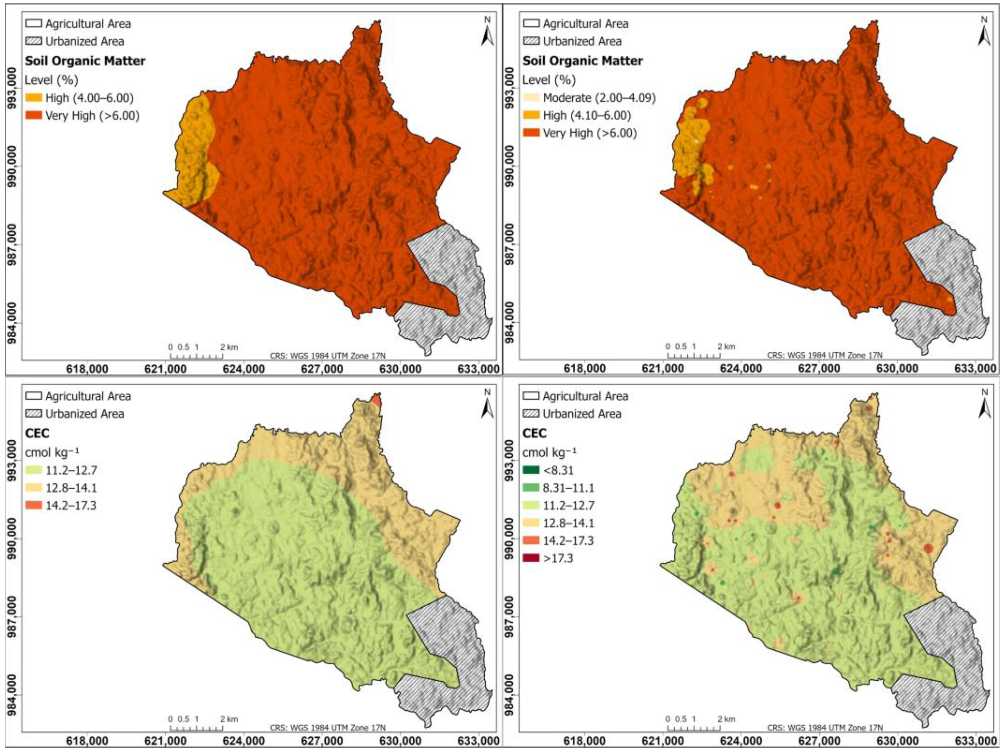
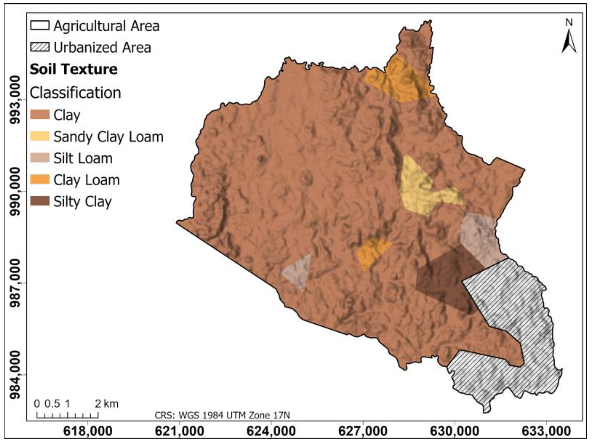

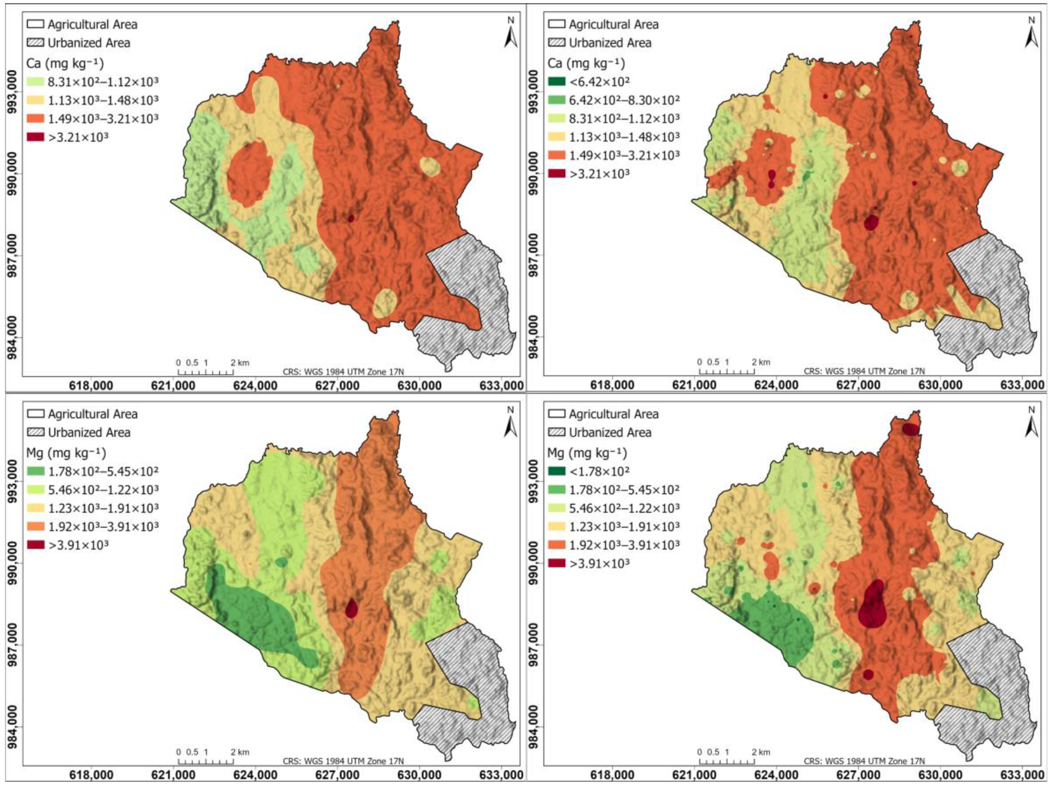
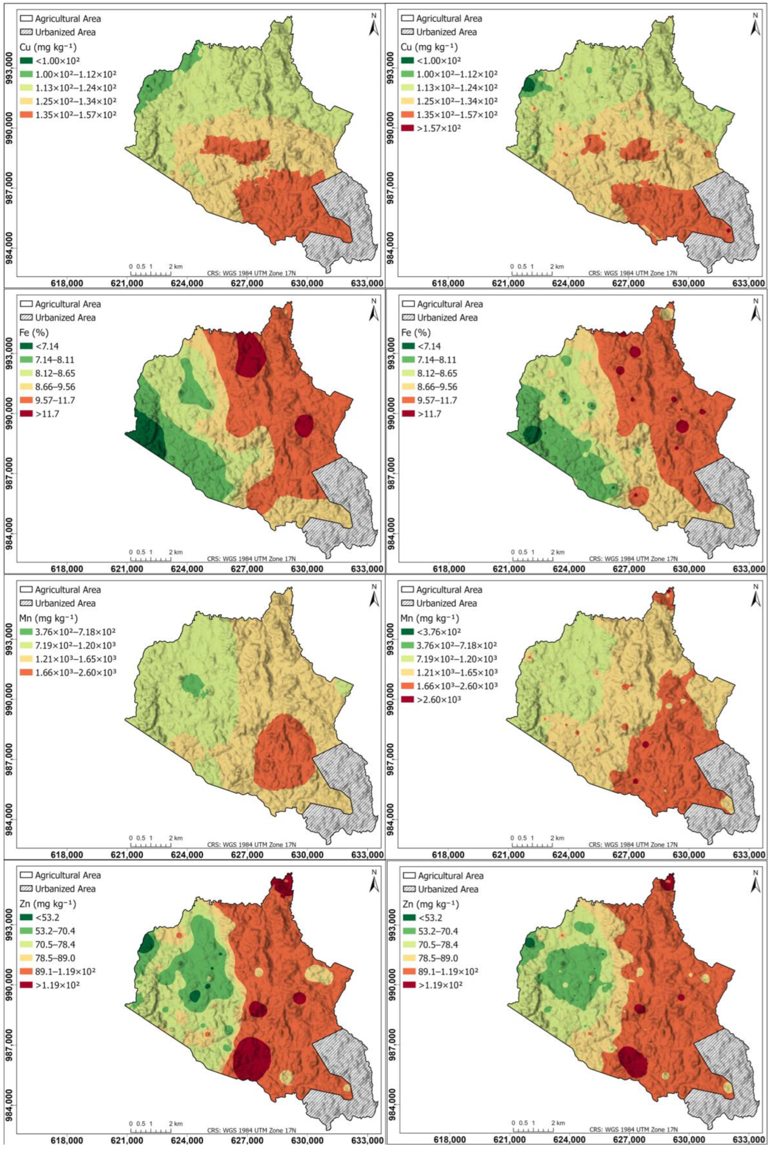
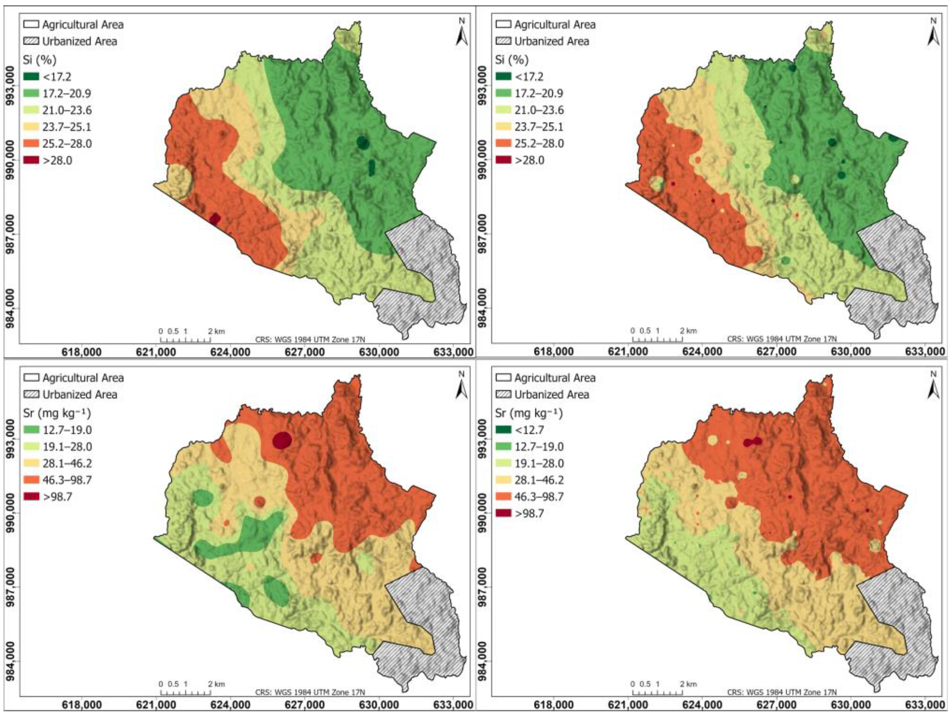
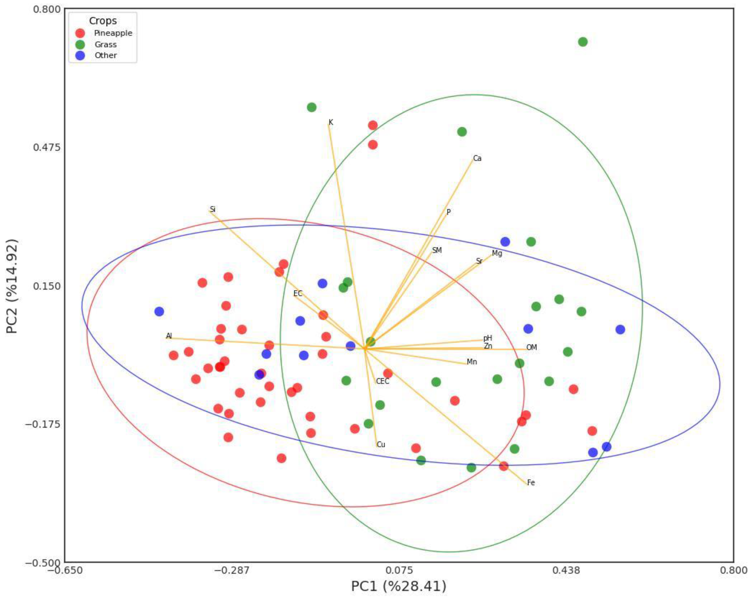
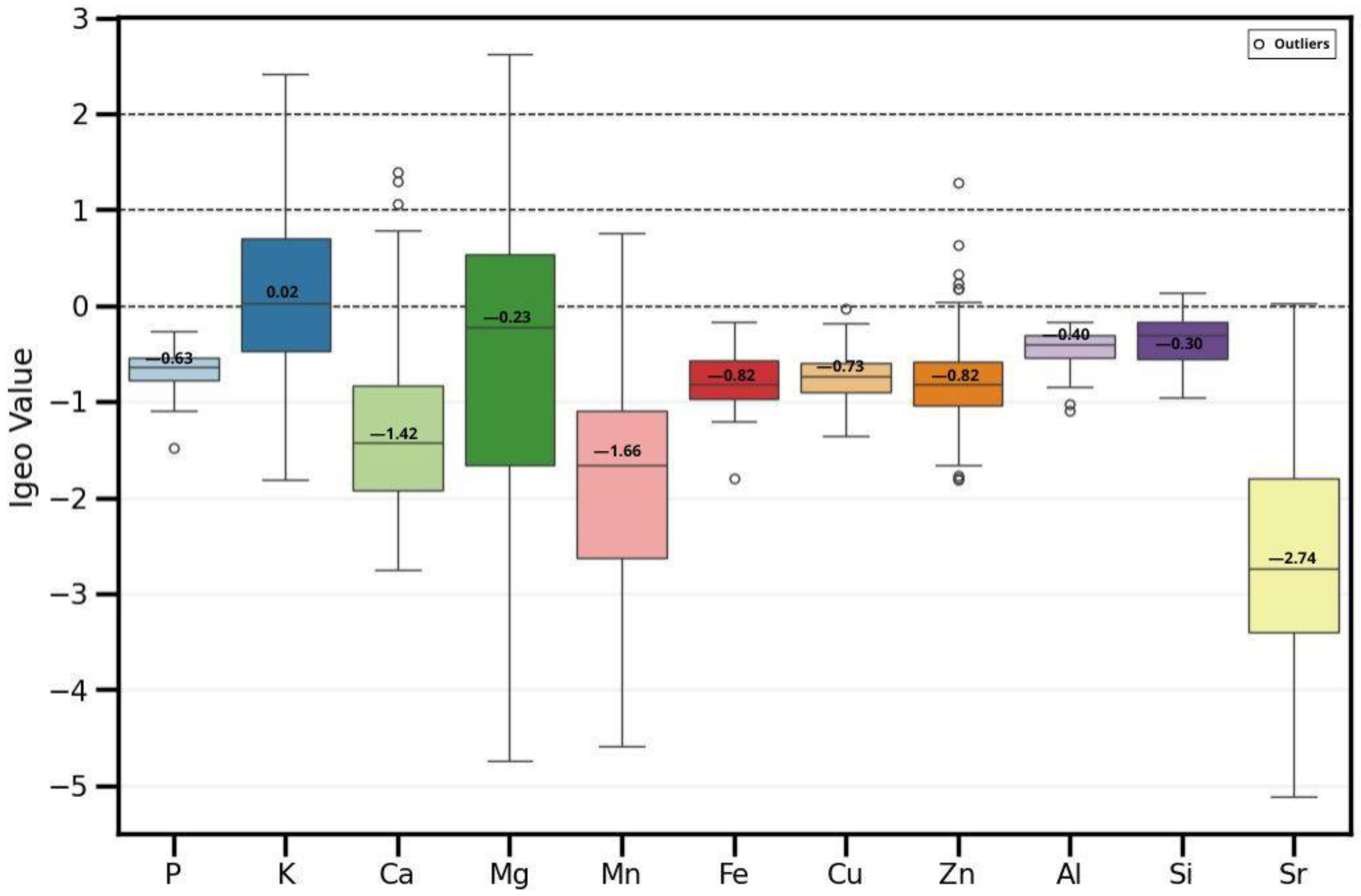

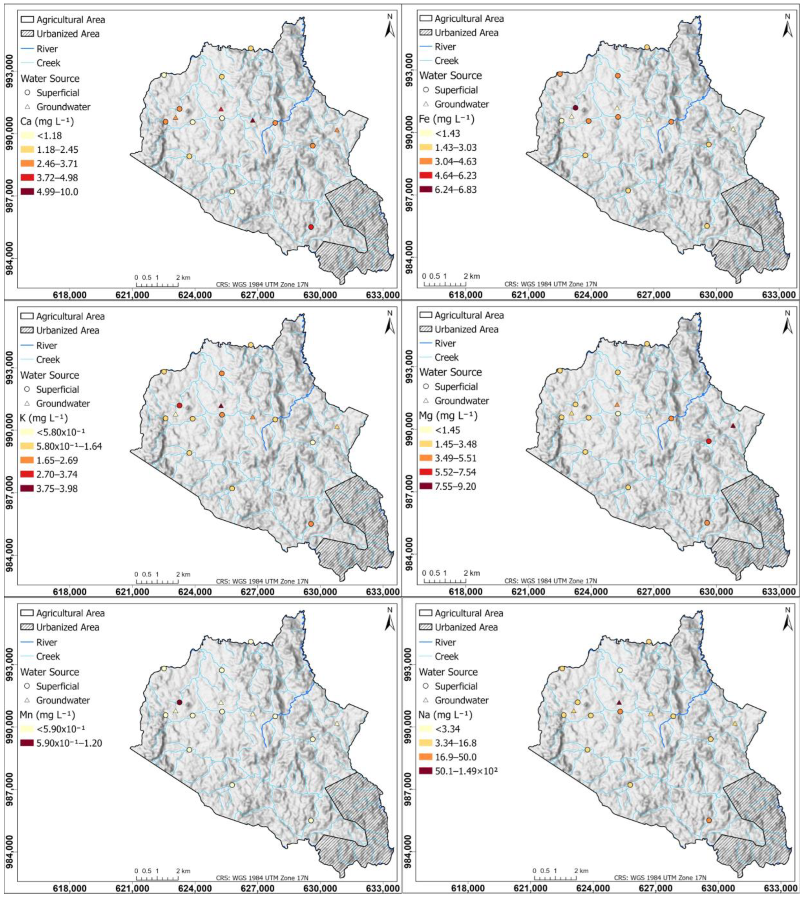
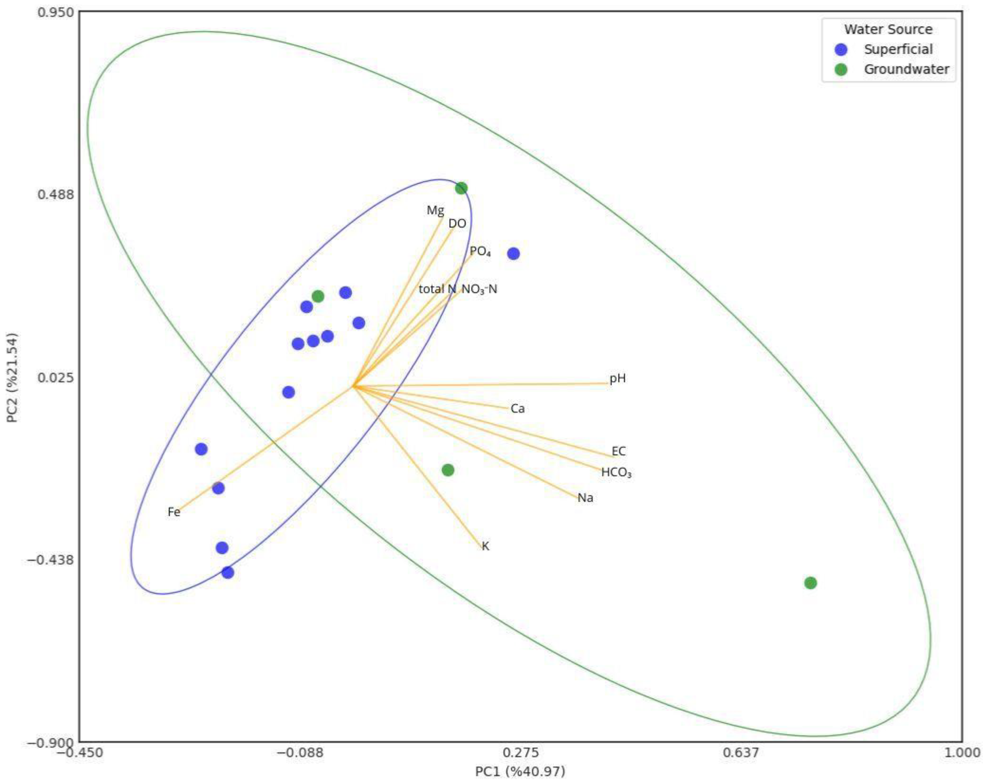
Disclaimer/Publisher’s Note: The statements, opinions and data contained in all publications are solely those of the individual author(s) and contributor(s) and not of MDPI and/or the editor(s). MDPI and/or the editor(s) disclaim responsibility for any injury to people or property resulting from any ideas, methods, instructions or products referred to in the content. |
© 2025 by the authors. Licensee MDPI, Basel, Switzerland. This article is an open access article distributed under the terms and conditions of the Creative Commons Attribution (CC BY) license (https://creativecommons.org/licenses/by/4.0/).