An Innovative Indoor Localization Method for Agricultural Robots Based on the NLOS Base Station Identification and IBKA-BP Integration

Abstract

This study proposes an innovative indoor localization algorithm based on the base station identification and improved black kite algorithm–backpropagation (IBKA-BP) integration to address the problem of low positioning accuracy in agricultural robots operating in agricultural greenhouses and breeding farms, where the Global Navigation Satellite System is unreliable due to weak or absent signals. First, the density peaks clustering (DPC) algorithm is applied to select a subset of line-of-sight (LOS) base stations with higher positioning accuracy for backpropagation neural network modeling. Next, the collected received signal strength indication (RSSI) data are processed using Kalman filtering and Min-Max normalization, suppressing signal fluctuations and accelerating the gradient descent convergence of the distance measurement model. Finally, the improved black kite algorithm (IBKA) is enhanced with tent chaotic mapping, a lens imaging reverse learning strategy, and the golden sine strategy to optimize the weights and biases of the BP neural network, developing an RSSI-based ranging algorithm using the IBKA-BP neural network. The experimental results demonstrate that the proposed algorithm can achieve a mean error of 16.34 cm, a standard deviation of 16.32 cm, and a root mean square error of 22.87 cm, indicating its significant potential for precise indoor localization of agricultural robots.

1. Introduction

The operational environment of agricultural robots is characterized by structural uncertainty and increasingly complex tasks, which makes localization and navigation essential technologies in modern robotics development [1,2,3,4]. The integration of advanced technologies, including the Internet of Things (IoT), emerging positioning systems, and artificial intelligence (AI), has provided significant advancements in the field of agricultural automation, particularly for the widespread implementation of machinery positioning and autonomous navigation systems in unmanned smart farming operations [5,6,7]. The Global Navigation Satellite System (GNSS) has been a cornerstone technology for intelligent agricultural machinery, achieving centimeter-level positioning accuracy [8] and enabling high-precision autonomous operations in various agricultural scenarios [9]. However, in complex environments, the GNSS signals often weaken or become entirely unavailable, which limits precise navigation and localization [10]. The Wi-Fi localization methods based on the received signal strength indication (RSSI) have received great attention for their simplicity, low cost, and wide coverage, providing a promising solution for improving the localization accuracy of agricultural robots in complex environments. The Wi-Fi indoor localization methods can be roughly classified into two categories: signal propagation model-based methods and fingerprinting-based methods [11,12,13,14]. The fingerprinting-based methods are costly to develop and maintain, which limits their practical application [15]. Therefore, this study explores the RSSI localization approach based on the signal propagation models tailored for agricultural robots in complex environments.

The non-line-of-sight (NLOS) conditions between the base stations and test points have consistently impeded the advancement of RSSI-based ranging technologies. To address these challenges, Cao et al. [16] proposed a Wi-Fi round-trip time (RTT) positioning method based on the line-of-sight (LOS) compensation and reliable NLOS identification. This method uses compensated LOS distances and credible NLOS distances for position estimation. Hou et al. [17] aimed to address poor UAV localization caused by the NLOS errors in UWB systems and proposed an improved UWB/MIMU integrated navigation method using an extended Kalman particle filter (EKPF), enhancing the positioning accuracy in the x, y, and z directions. Kong et al. [18] proposed an improved Dung Beetle Optimizer-enhanced CNN (IDBO-CNN) model, employing chaotic mapping and variational strategies to optimize hyperparameters, which increased the NLOS identification F1-score by 3.31% in UWB localization compared to the conventional CNN models. However, these studies did not consider the impact of selecting different subsets of Wi-Fi base stations on localization accuracy. Therefore, datasets used to train neural networks might include signals from unreliable base stations, thus reducing the overall precision of localization.

Traditional RSSI-based ranging positioning algorithms often depend on empirical parameters to construct path loss models [19,20,21]. However, complex and dynamic working environments of agricultural robots can introduce significant deviations during the model construction process, leading to substantial positioning errors [22]. To overcome this limitation, recent studies have increasingly implemented neural networks into positioning algorithms. Zhao et al. [23] used the backpropagation (BP) neural networks to develop a path loss model for signal propagation, thus achieving coarse localization of target nodes. Tian et al. [24] proposed a KF–LSTM algorithm combining Kalman filtering with LSTM to enhance the UWB indoor positioning accuracy. The results indicated superior performance and stability of the proposed model over the BP, KF-BP, and LSTM models, particularly in noisy environments. However, despite significant advancements, the RSSI-based ranging algorithms face three major challenges.

(1) in complex agricultural environments, dynamic obstacles, such as crop canopies, greenhouse structures, and undulating terrain, aggravate NLOS-induced positioning errors, thus significantly degrading localization accuracy.

(2) although the BP neural network-based ranging models can achieve high precision, their performance is often compromised by randomly initialized weights and biases, which might make the model fall into local optima.

(3) although the integration of optimization algorithms can improve the accuracy of BP neural network models to a certain extent, it still faces some limitations in agricultural environments, including insufficient global search capability and suboptimal convergence precision.

In addressing the aforementioned challenges, this study proposes an agricultural robot positioning algorithm integrating the base station screening technique and an IBKA-BP fusion approach. The proposed algorithm starts by partitioning base stations into subsets tailored to agricultural operational scenarios (e.g., orchard row navigation, greenhouse dense occlusion, and cross-regional field operations). Through the spatiotemporal analysis of NLOS signals in farmland environments, subsets containing NLOS base stations are excluded as they can generate clustered estimated positions. In addition, dense clusters are identified to compute centroids for reliable positioning, whereas NLOS-inducing base stations are detected by analyzing their frequency using valid data. Further, a dynamic blacklisting mechanism is implemented to mitigate transient NLOS interference caused by mobile obstacles (e.g., harvesters or irrigation equipment). Moreover, RSSI samples from the LOS base stations are processed by the Kalman filtering and Min-Max normalization operations to suppress signal fluctuations induced by abrupt environmental changes (e.g., humidity shifts or metallic machinery reflections). The BP neural network is then employed to model a nonlinear relationship between the RSSI and distance values, thus effectively addressing the dependence on agricultural-specific parameters, such as soil permittivity and vegetation density. Furthermore, to enhance the BP neural network’s performance, the improved black kite algorithm (IBKA) incorporates tent chaotic mapping, lens imaging reverse learning, and golden sine strategies. In addition, by optimizing the initial weights and biases using the IBKA, a robust RSSI ranging model is constructed, explicitly addressing the problem of spatial-temporal variability of agricultural environments. The results of the experimental tests conducted in the greenhouse indicate that the proposed IBKA-BP algorithm can achieve the mean error (ME), standard deviation (STD), and root mean square error (RMSE) values of 16.34 cm, 16.32 cm, and 22.87 cm, respectively, which are significantly lower than those of the existing algorithms. Finally, the proposed algorithm demonstrates the fastest convergence speed among all comparison algorithms, which confirms its effectiveness in agricultural environments.

2. Algorithm Design Process

2.1. Base Station Filtering Algorithm

The first step to address the presence of unreliable NLOS base stations involves dividing them into several subsets. The estimated positions derived from the RSS subset that exclude the NLOS base stations typically form dense clusters. Based on this observation, the estimated positions are grouped into clusters. Dense clusters are identified, and their centroid positions are returned to obtain reliable positioning results. In addition, the frequencies of all base stations in the reliable results are analyzed to identify the NLOS base stations.

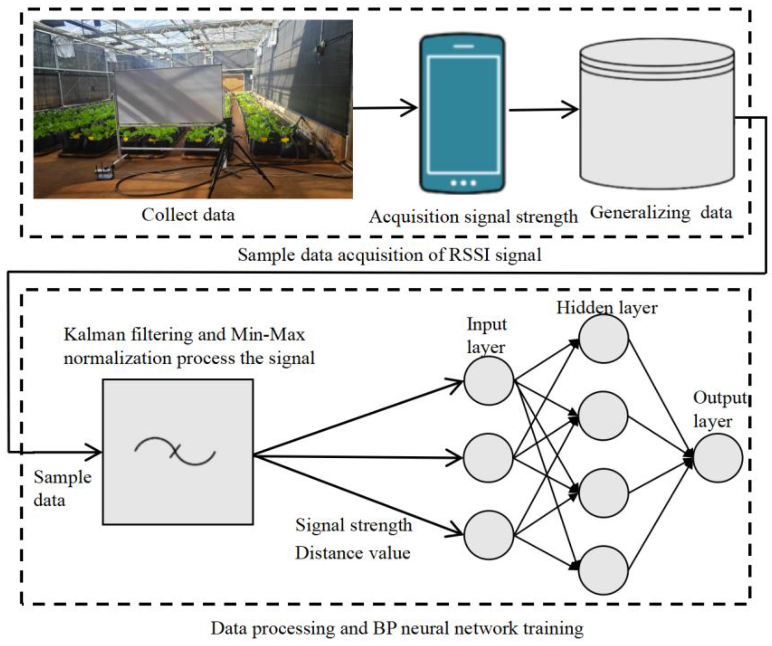
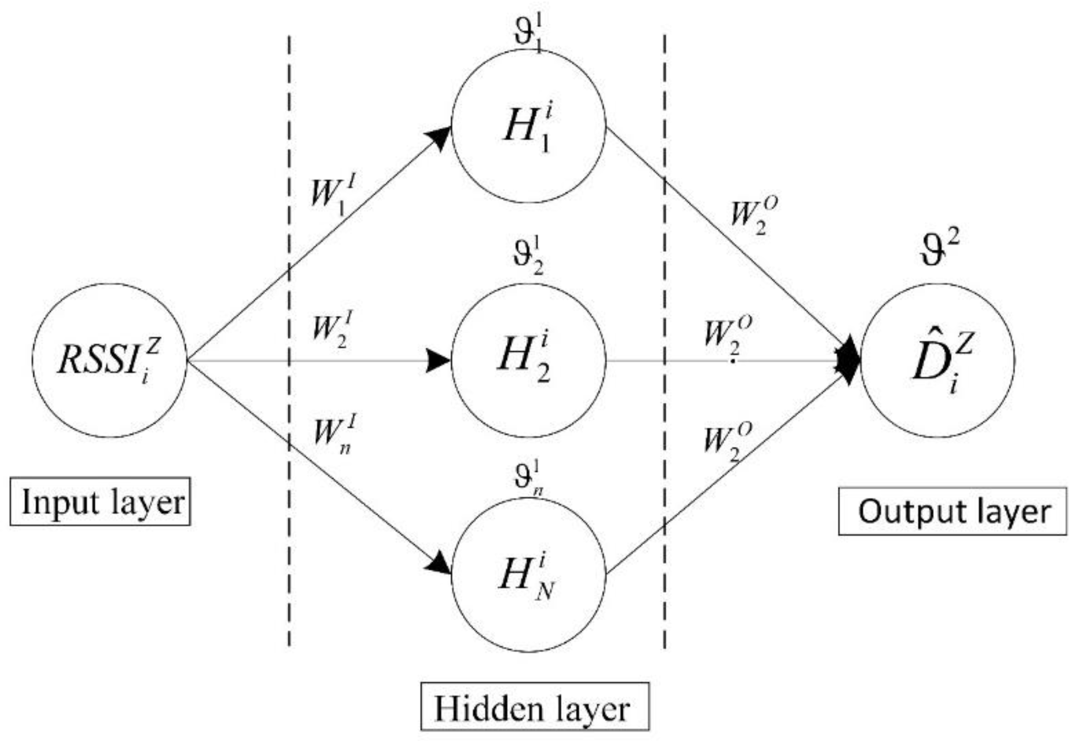
2.2. Distance Measurement Model Based on BP Neural Network

Classical indoor positioning algorithms based on the RSSI often depend on empirical parameters to construct path loss models. However, these parameters are susceptible to environmental noise, which can introduce significant errors and reduce positioning accuracy. However, to overcome these limitations, this study constructs a distance measurement model using a BP neural network. The RSSI data are processed by Kalman filtering and Min-Max normalization to suppress signal fluctuations and accelerate convergence during gradient descent in the distance measurement model. This approach can effectively capture the relationship between RSSI and distance in complex environments, significantly enhancing positioning accuracy.

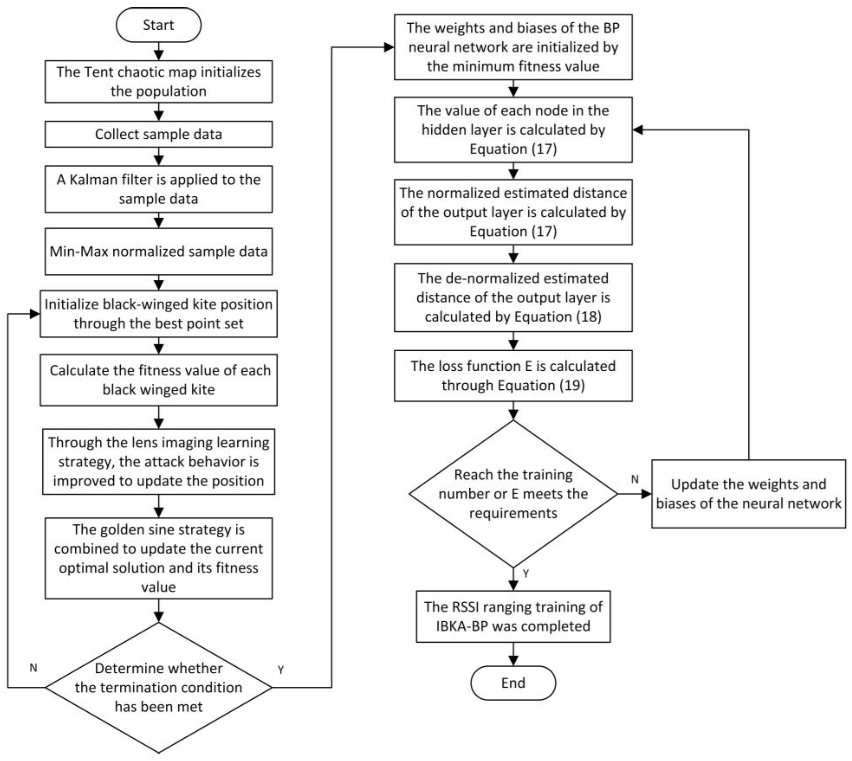
2.3. IBKA-BP Neural Network RSSI Distance Measurement Algorithm

To further improve indoor positioning accuracy, this study integrates the IBKA with the RSSI distance measurement algorithm based on a BP neural network. The IBKA improves the black kite optimization algorithm by improving its search efficiency and ability to select optimal weights and thresholds. Further improvements to the black kite algorithm involve key modifications to its structure to improve its performance in optimizing the BP neural network. Then, chaos mapping is used to generate uniformly distributed initial individuals, enhancing population diversity. In addition, a lens imaging reverse learning strategy is employed to improve the algorithm’s stability and robustness. Further, during the attack and migration phases, a golden sine strategy is introduced, which partitions the solution space based on the golden ratio. This approach refines the positions of black kites, thus allowing for more precise and accurate positioning results.

The proposed method for RSSI distance measurement based on a BP neural network is illustrated in Figure 1. First, the RSSI signal strength and distance relationships are collected as data samples in the experimental environment. Next, these samples are processed by Kalman filtering and Min-Max normalization and then input into the BP neural network for training. During position prediction, the signal strength values collected from the test point are fed to the trained network, which outputs the predicted position of the test point.

3. NLOS Base Station Identification Algorithm

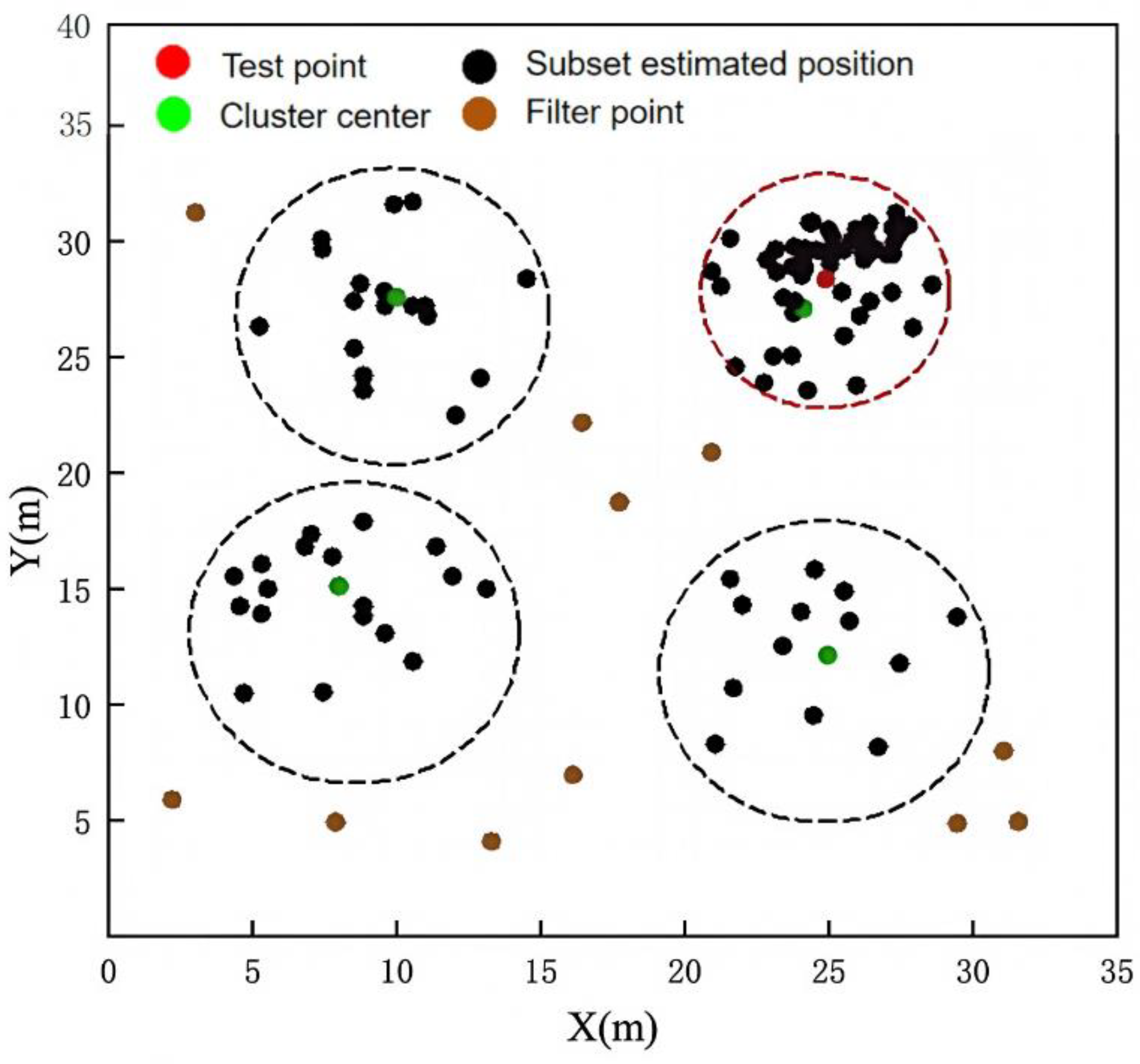
3.1. Subset Division

This study uses a set of Wi-Fi base stations denoted by M, consisting of two subsets: a subset N₁ that represents the NLOS base stations and a subset N₂ that indicates the LOS base stations. The relationship between the two subsets is defined as follows: |N₁| + |N₂| = |M|.

Two key phenomena are observed:

(1) When all three selected base stations are from subset N₂, the ranging results are accurate with minimal discrepancies. Any combination of three base stations from N₂ yields effective positioning results. The total number of subsets consisting entirely of base stations from N₂ is m₁ = C (N₂, 3);

(2) Due to the obstruction effects affecting the signals of NLOS base stations, significant random-ranging interference can occur. When randomly selecting n₂ < 3 base stations from subset N₂ and n₁ = 3 − n₂ base stations from N₁ to form subsets for positioning, the resulting subsets exhibit high dispersion [25]. The total number of such subsets is m₂ = C(M, 3) − C(N₂, 3).

Based on these observations, set M is divided into multiple subsets to obtain positioning results. Subsets containing NLOS base stations are subsequently filtered out by evaluating the concentration of their positioning results.

3.2. Density Peak Detection and Target Localization

Using the generated RSS subset samples, the received RSSI values are transformed into distance values for each subset using a path loss model, thus enabling trilateration-based positioning of the subsets.

This study employs the logarithmic normal path loss model, which has been widely used in indoor positioning algorithms. This model is mathematically expressed as follows [26]:

$$PL(d)=PL(d_0)+10\eta ·log\left({\displaystyle \frac{d}{d_0}}\right)+X_{\sigma }$$

(1)

where $PL(d)$ and $PL(d_0)$ represent the path loss at a distance $d$, expressed in meters, and a distance $d_0$, also expressed in meters, from the base station, respectively, $d_0$ is typically 1 m; $X_{\sigma }$ represents shadow fading, which follows a normal distribution; $\eta$ is the path loss exponent, which is dependent on the environment.

The RSSI value received at a distance $d$ (in meters) from the base station can be expressed as follows:

$$RSSI(d)=P_t-PL(d)$$

(2)

where $P_t$ denotes the transmitted signal power.

By substituting Equation (1) into Equation (2), the relationship between the RSSI and distance can be expressed by:

$$RSSI(d)=A-10\eta ·log10\left({\displaystyle \frac{d}{d_0}}\right)-x_{\sigma }$$

(3)

where A represents the RSSI value at a reference distance $d_0$, and $A=P_t-PL\left(d_0\right)$.

Based on this relationship, the estimated distance from the base station to the test point can be determined, and each $d_{ijk}$ can be used to estimate the location of the test point. Consequently, a localization subset $m$ comprising all test point localization results can be defined by:

$$\left[d_{123},d_{124},\cdots ,d_{ijk},\cdots \right],\left|d_{ijk}\right|=3$$

(4)

where,

$$d_{ijk}=\left[d_i,d_j,d_k\right],i,j,k=1,2,\cdots ,m$$

where $d_{ijk}$ can be used to estimate the position of a test point, and the localization subset composed of all $m$ test point localization yields $l{u}_{sub}$, which is defined as $l{u}_{sub}=\left[l{u}_1,l{u}_2,\cdots ,l{u}_m\right]$, where $l{u}_i$ represents the localization result calculated from the ith distance subset.

Considering the high dispersion of positioning results and the presence of a preset constant number of NLOS base station clusters, this study employs the density peaks clustering (DPC) [27] algorithm to identify the densest clusters. Specifically, the DPC uses $l{u}_{sub}$ and cuts off the distance $d_c$ as input. It also assumes that neighbors with lower local densities are surrounded by cluster centers and are relatively far from any points with higher local densities. First, the DPC calculates the values of a spatial distance $l{u}_i$ between $l{u}_j$ data points, denoted as $dis(i,j)$, which represents the separation between a particular point and the other points with higher densities:

$$dis(i,j)=‖l{u}_i-l{u}_j‖,i,j=1,2,\cdots ,m$$

(5)

In this study, the Euclidean distance is used to measure the spatial separation between data points. The fundamental premise of the DPC defines that cluster centers should simultaneously exhibit two critical characteristics: high local density (being surrounded by numerous neighboring points) and substantial separation from points with higher density. By defining a pairwise distance matrix for all data points, this approach can establish the necessary foundation for subsequent density estimation and relative distance analysis. Next, the local density for each point is determined. The local density of $l{u}_i$, denoted by ${\rho }_i$, is defined as follows:

$${\rho }_{\mathrm{i}}={\displaystyle \sum _j\mathrm{\Omega }\left(dis\left(i,j\right)-d_c\right)}$$

(6)

Then, it can be written that:

$$\mathrm{\Omega }(x)=\left\{\begin{array}{ll}1,& if x<0\\ 0,& otherwise\end{array}\right.$$

(7)

Similarly, the local density $\rho$ for all subset locations is calculated. Based on the obtained local densities, the DPC algorithm computes a relative minimum distance $\delta$ for each estimated result. The relative minimum distance of $l{u}_i$, denoted by ${\delta }_i$, is defined as follows:

$${\delta }_i=\underset{j:{\rho }_j>{\rho }_{\mathrm{i}}}{\min }(d_{ij})$$

(8)

Points with high $\rho$ and $\delta$ values are selected as cluster centers, whereas points with low $\rho$ value but high $\delta$ value are identified as outliers; the remaining points are assigned to clusters based on their proximity to the cluster centers.

Figure 2 shows an example where three base stations are randomly selected from the total set of base stations (|M| = 10), and the estimated test point locations are provided. The DPC algorithm divides these results into four clusters, where red circles denote clusters with smaller mutual Euclidean distances between the positioning results, and black circles represent clusters with larger mutual Euclidean distances, as shown in Figure 2.

Environmental obstacles can cause significant deviations in the distances associated with NLOS base stations. Consequently, the RSS subset localization results without the NLOS base stations are closer to the true position, having the smallest mutual Euclidean distances. Conversely, as the number of NLOS base stations increases, the dispersion of the RSS subset localization results also increases.

In this study, the most reliable localization subset was identified by determining the dispersion of each cluster based on the mutual Euclidean distances between the subset localization results within a cluster. Particularly, this process involves computing the average of all pairwise Euclidean distances for the localization results in each cluster. The cluster with the smallest average Euclidean distance, indicating the least dispersion, is selected as a reliable subset. In Figure 2, the reliable localization subset is highlighted by the red circle.

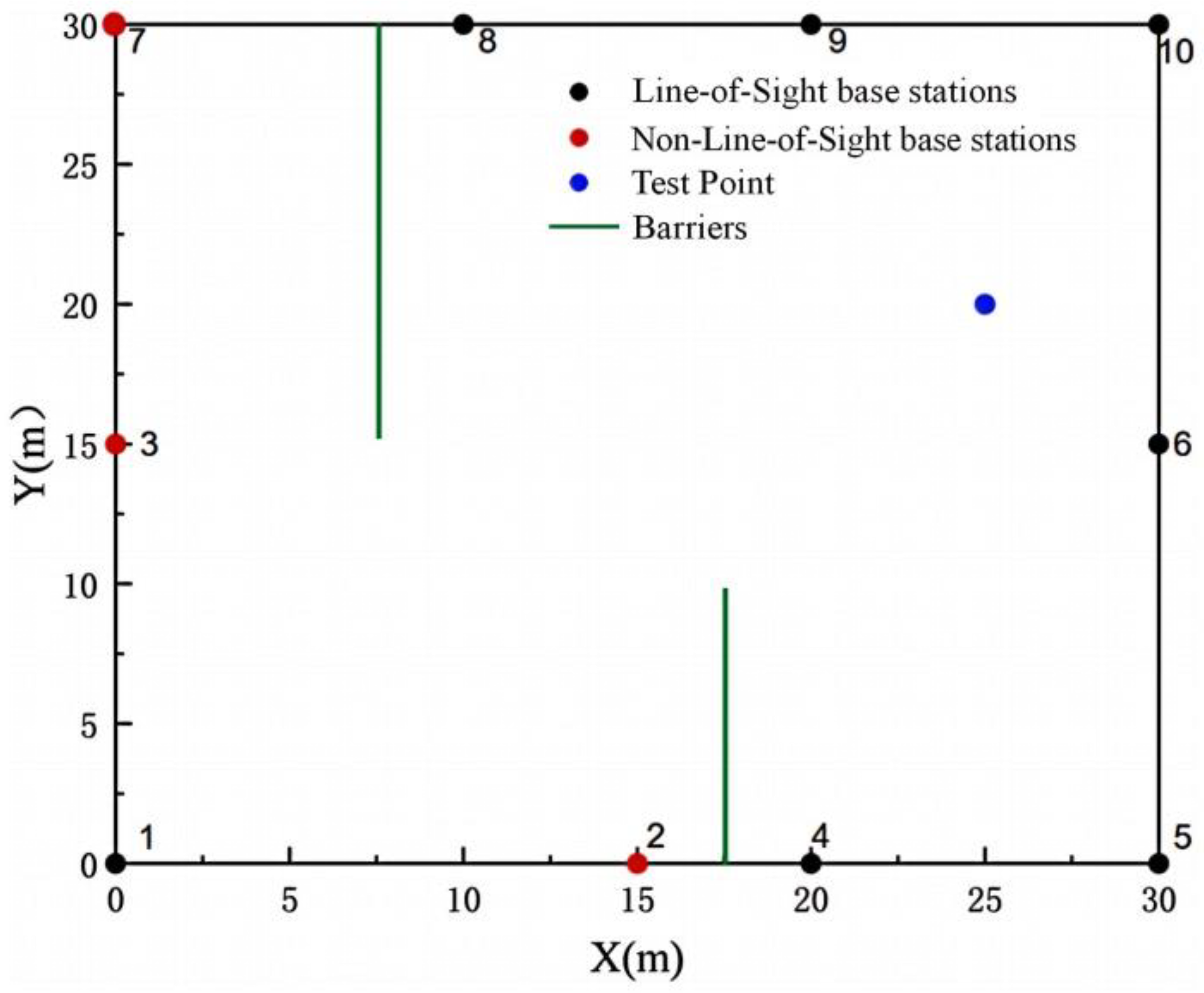
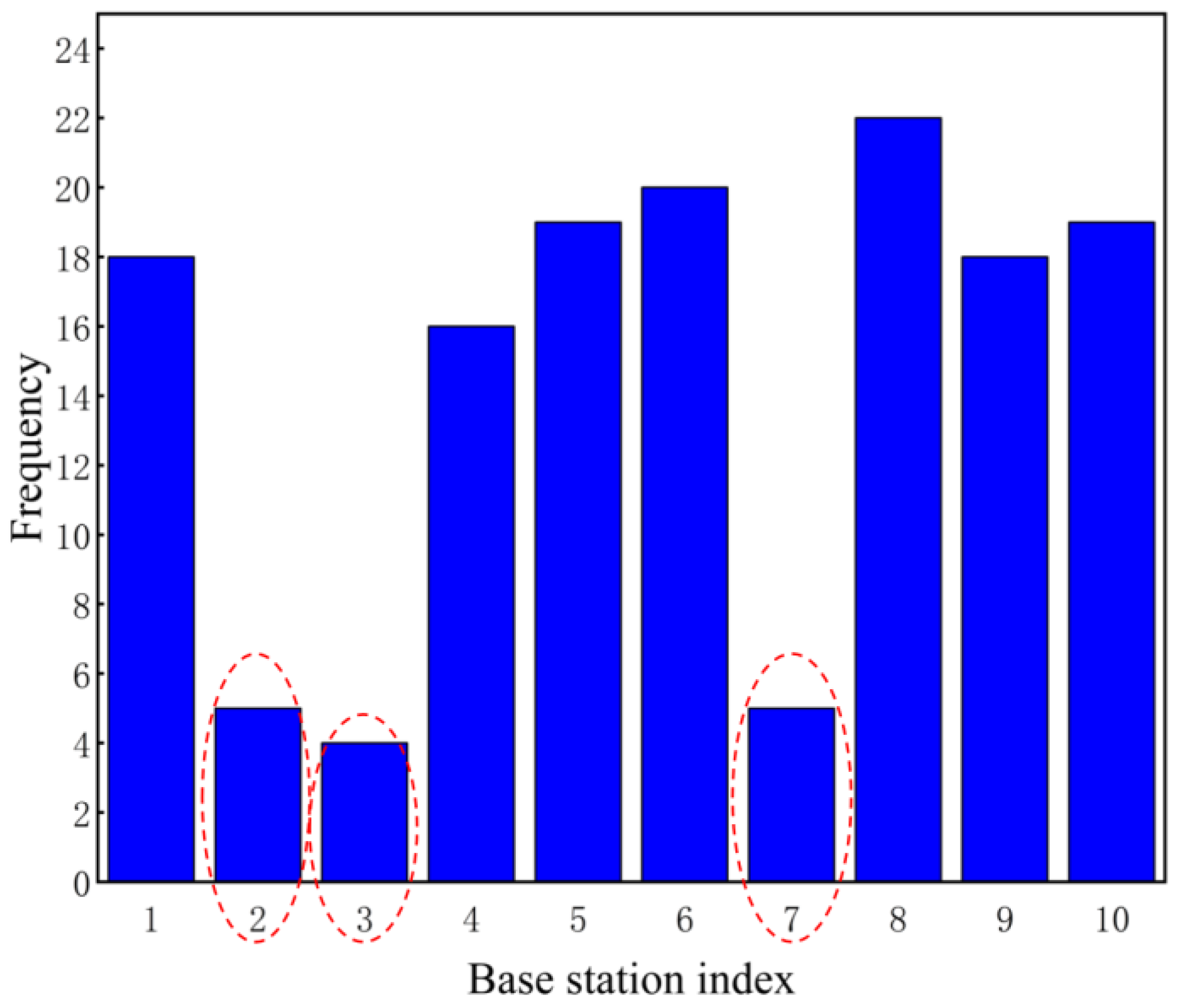
3.3. NLOS Base Station Identification

In identifying NLOS base stations, which are typically characterized by unreliable results, it is crucial to calculate the frequency of each base station’s appearance in reliable localization data. In this study, base stations are categorized into two groups; namely, base stations with higher occurrence frequencies in reliable results are classified as LOS base stations, and those with lower occurrence frequencies are identified as NLOS base stations. In essence, a higher frequency of a base station in the reliable positioning results increases the likelihood of the base station being a LOS base station.

The simulation environment used for this study is illustrated in Figure 3, where it can be seen that 10 base stations were distributed around a 30 m × 30 m square. A test point was located at coordinates (25, 20). Two obstacles were included in the simulation environment, represented by green lines in Figure 3, measuring 15 m and 10 m, which impeded signal propagation. The base stations located at (15, 0), (0, 15), and (0, 30) had their signals obstructed, and the remaining seven base stations, placed at (0, 0), (20, 0), (30, 0), (30, 15), (10, 30), (20, 30), and (30, 30) had unobstructed signals. As displayed in Figure 4, the frequency-based identification algorithm could effectively highlight the NLOS base stations. In the reliable positioning results, base stations 2, 3, and 7 appeared less frequently than the others, confirming their classification as NLOS base stations.

4. Distance Measurement Model Based on BP Neural Network

Based on Equation (3), the parameters significantly affect the RSSI-distance relationship, leading to a low positioning accuracy in conventional path loss models [28]. In contrast to the classical indoor positioning algorithms based on RSSI ranging, neural networks excel at capturing nonlinear relationships and reducing the impact of environmental noise on the positioning result [29]. Consequently, this study designs an RSSI distance measurement model using a BP neural network. This approach suppresses fluctuations in the RSSI data and eliminates dependence on the environmental parameters. In the BP neural network distance measurement model, the RSSI value received by a base station represents an independent variable, whereas the distance between the base station and the test point denotes a dependent variable. The sample data for the RSSI ranging algorithm are defined as follows:

$$\left\{\begin{array}{l}{X}_{in}=[RSS{I}_{1}RSS{I}_2\cdots {\left.RSS{I}_n\right]}^T\\ X_{out}={\left[D_1{D}_2\cdots D_{\mathrm{n}}\right]}^T\end{array}\right.$$

(9)

where $X_{\mathrm{in}}$ represents the input sample vector, $X_{\mathrm{out}}$ represents the output sample vector, and n denotes the total number of samples; $D_{\mathrm{i}}$ indicates the distance between the test point and the base station; $RSS{I}_{\mathrm{i}}$ is the signal strength value received at point i.

In minimizing unnecessary noise included in the RSSI measurements, the Kalman filtering algorithm [30] is first applied to the raw RSSI data to reduce noise fluctuations and signal attenuation. The RSSI dataset values of the target node are denoted by $y\left(n\right)$ and used to calculate the estimated RSSI values for n points $x\left(\mathrm{n}\right)$. The Kalman filter estimation process can be expressed as follows:

$$\left\{\begin{array}{l}x\left(n\right)=\phi x\left(n-1\right)+{\omega }_x\left(n-1\right)\\ y\left(n\right)=Hx\left(n-1\right)+Z\left(n\right)\end{array}\right.$$

(10)

where $x\left(n-1\right)$ is the previous RSSI value estimated at a position $\left(n-1\right)$; $y\left(n\right)$ represents the estimated RSSI value at a position n; $\phi$ is the state transition matrix; $H$ is the measurement matrix; ${\omega }_x\left(n-1\right)$ denotes the white noise added at a position $\left(n-1\right)$; $Z\left(n\right)$ represents the measurement noise at a position n.

The Kalman filtering process involves two steps. The first step is the prediction step, where the estimated RSSI value at a point n is obtained by:

$$\widehat{x}\left(n/n-1\right)=\phi x\left(n-1\right)$$

(11)

The covariance error of the RSSI at a point n is calculated by:

$${\widehat{p}}_x\left(n/n-1\right)=\phi p_x\left(n-1\right){\phi }^T+Q_x\left(n-1\right)$$

(12)

where $p_x\left(n-1\right)$ is the covariance error at a positioning location $(n-1)$, ${\phi }^T$ represents the transpose of the state transition matrix, and $Q_x\left(n-1\right)$ indicates the variance error at a location $(n-1)$.

Subsequently, based on Equations (11) and (12), a covariance error $P_x\left(n\right)$ can be expressed as follows:

$$P_x\left(n\right)=\left(I-K_x\left(n\right)H\right){\widehat{P}}_x\left(n/n-1\right)$$

(13)

A gain error $K_x\left(n\right)$ at a location n is computed as follows:

$$K_x\left(n\right)={\widehat{p}}_x\left(n/n-1\right)H^T{\left[H{\widehat{P}}_x\left(n/n-1\right)H^T+R_x\right]}^{-1}$$

(14)

where $R_x$ represents the noise covariance error of a system.

Finally, after Kalman filtering, the estimated RSSI value at point n is updated as follows:

$$x\left(n\right)=\widehat{x}\left(n/n-1\right)+K\left(n\right)\left[y\left(n\right)-H\widehat{x}\left(n/n-1\right)\right]$$

(15)

The covariance matrix indicates the uncertainty inherent in the state estimation process. Through its recursive update mechanism, the Kalman filter can provide statistically optimal estimates by systematically minimizing the posterior estimation error covariance in each iteration. Applying Kalman filtering reduces random noise caused by environmental and device interference [31] while smoothing the RSSI fluctuations and thus improving the accuracy of the RSSI ranging mode l [32]. After Kalman filtering, the sample data undergo Min-Max normalization [33], defined by Equation (16), to accelerate convergence in the gradient descent method.

$$\left\{\begin{array}{l}RSS{I}_i^Z={\displaystyle \frac{RSS{I}_i-RSS{I}^{Min}}{RSS{I}^{Max}-RSS{I}^{Min}}}\\ D_i^Z={\displaystyle \frac{D_i-D^{Min}}{D^{Max}-D^{Min}}}\end{array}\right.$$

(16)

In Equation (16), $RSS{I}_i^Z$ and $D_i^Z$ represent the values after Min-Max normalization; $RSS{I}^{Max}$ and $RSS{I}^{Min}$ are the maximum and minimum values of the input sample vector, respectively; $D^{Min}$ and $D^{Max}$ are the minimum and maximum values of the output sample vector, respectively.

The BP neural network model shown in Figure 5 consists of three layers: an input layer, a hidden layer, and an output layer. In preventing overfitting, the hidden layer is limited to a single layer [34], and the number of nodes in this layer is determined by an empirical formula [35]. The network takes the $RSS{I}_i^Z$ data as input and generates ${\widehat{D}}_i^Z$ values as output. The weights connecting the input to the hidden layer are denoted by $W^I=\left[W_1^I,W_2^I\cdots ,W_n^I\right]$, where $W^O=\left[W_1^O,W_2^O\cdots ,W_n^O\right]$ indicates the connection weights from the hidden layer to the output layer.

The value of the Kth node in the hidden layer is represented as $H_k^i\left(k=1,2,\cdots ,N\right)$, and the biases of node K in the hidden and output layers are denoted by ${\vartheta }_k^1$ and ${\vartheta }_k^1$, respectively. A proper adjustment of the connection weights and biases can significantly improve the precision of positioning accuracy. The hidden layer’s nodes $H_j^i$ and the model’s RSSI estimated values ${\widehat{D}}_i^Z$ are respectively expressed as follows:

$$\left\{\begin{array}{l}{H}_k^i={\displaystyle \frac{2}{1+e^{-2\left(w_k^1\times RSS{I}_i^Z-{\vartheta }_k^1\right)}}}-1\\ {\widehat{D}}_i^Z={\displaystyle \sum _{j=1}^N\left(W_k^2\times H_k^i\right)}-{\vartheta }^2\end{array}\right.$$

(17)

The estimated distance value obtained by denormalization is obtained by:

$${\widehat{D}}_i={\widehat{D}}_i^z\left(D^{Max}-D^{Min}\right)+D^{Min}$$

(18)

The loss function E is defined by:

$$E={\displaystyle \sum _i^S{E}_i}={{\displaystyle \sum _{i=1}^S\frac{1}{2}\left({\widehat{D}}_i^z-D_i^z\right)}}^2$$

(19)

where $E_i$ represents the loss function of the ith sample.

In the proposed distance localization model, the weights and biases of the BP neural network are iteratively updated to minimize the value of a loss function E [36]. During the model training process, when the E value reaches a predefined threshold or the maximum number of iterations is achieved, the final weights and biases of the neural network are determined. The RSSI value is used as input and normalized using Equation (16) to produce $RSS{I}^z$. Then, the distance is estimated using Equation (17), followed by denormalization performed by Equation (18) to obtain the final distance estimate denoted by $\widehat{D}$. Finally, by using Equation (19) to measure the error between the model’s predicted outputs and the actual target values, the proposed model’s performance can be iteratively refined for greater accuracy.

5. IBKA-BP Neural Network RSSI Ranging Algorithm

5.1. Black Kite Algorithm

The black kite optimization algorithm was first introduced by Wang et al. [37] in 2024. This advanced meta-heuristic algorithm has been inspired by the migration and predation behaviors of black kites in nature. Namely, by simulating the high adaptability of black kites to environmental changes and target locations, this algorithm incorporates the Cauchy mutation strategy [38] and the Leader strategy [39] to enhance global search capability and convergence speed.

In this algorithm, the initialization process begins by establishing random solutions. The position of each black kite is defined as shown as:

$$BK=\left[\begin{array}{ccccc}B{K}_{1,1}& B{K}_{1,2}& \cdots & \cdots & B{K}_{1,dim}\\ B{K}_{2,1}& B{K}_{2,2}& \cdots & \cdots & B{K}_{1,dim}\\ ⋮& ⋮& ⋮& ⋮& ⋮\\ ⋮& ⋮& ⋮& ⋮& ⋮\\ B{K}_{pop,1}& B{K}_{pop,2}& \cdots & \cdots & B{K}_{pop,dim}\end{array}\right]$$

(20)

where $B{K}_{ij}$ represents the jth dimension of the ith Black Kite, $pop$ is the number of solutions, and $dim$ denotes the dimensionality of the problem.

The black kite optimization algorithm ensures the even distribution of the initial positions using the following expression:

$$X_i=B{K}_{lb}+rand(B{K}_{ub}-B{K}_{lb})$$

(21)

where i is an integer between one and $pop$; $B{K}_{lb}$ and $B{K}_{ub}$ are the lower and upper bounds of the ith black kite in the jth dimension, respectively; $rand$ represents a randomly selected value between zero and one.

During initialization, the IBKA designates the individual with the best fitness value as a leader X_L, representing the optimal position in the population.

The best fitness is expressed as follows:

$$f_{best}=min\left(f\left(X_i\right)\right)$$

(22)

Therefore, the initial leader is defined by:

$$X_L=X\left(find\left(f_{best}=f\left(X_i\right)\right)\right)$$

(23)

$$y_{t+1}^{i,j}=\left\{\begin{array}{l}{y}_t^{i,j}+n(1+sin(r))\times y_t^{i,j},p<r\\ y_t^{i,j}+n\times (2r-1)\times y_t^{i,j},else\end{array}\right.$$

(24)

$$n=0.05\times e^{-2\times {\left({\displaystyle \frac{t}{T}}\right)}^2}$$

(25)

where $y_t^{i,j}$ and $y_{t+1}^{i,j}$ represent the positions of the ith black kite in the jth dimension at iterations t and (t + 1), respectively; r is a random number within the [0, 1] range; $p$ is a constant value of 0.9; $T$ denotes the total number of iterations; $t$ represents the current iteration count.

The model can also be expressed as:

$$y_{t+1}^{i,j}=\left\{\begin{array}{l}{y}_t^{i,j}+C\left(0,1\right)\times \left(y_t^{i,j}-L_t^j\right),F_i<F_{ri}\\ y_t^{i,j}+C\left(0,1\right)\times \left(L_t^j-m\times y_t^{i,j}\right),else\end{array}\right.$$

(26)

$$m=2\times sin\left(r+{\displaystyle \frac{\pi }{2}}\right)$$

(27)

where $L_t^j$ represents the score of the black kite leader in the jth dimension up to the tth iteration; $F_i$ indicates the position of an individual black kite in the jth dimension during the tth iteration process; $F_{ri}$ is the obtained fitness value; $C(0,1)$ signifies $cauchy$ mutation, which can be mathematically modeled as follows:

$$f\left(x,\delta ,\mu \right)={\displaystyle \frac{1}{\pi }}{\displaystyle \frac{\delta }{{\delta }^2+{\left(x-\mu \right)}^2}},-\infty <x<\infty$$

(28)

When δ = 1 and μ = 0, the mathematical model for Cauchy mutation becomes:

$$f\left(x,\delta ,\mu \right)={\displaystyle \frac{1}{\pi }}{\displaystyle \frac{1}{x^2+1}},-\infty <x<\infty$$

(29)

5.2. Heuristic Algorithm Improvement Strategy Inspired by Black-Winged Kite

In this study, the tent Map chaotic mapping is introduced to initialize the algorithm population [40]. This approach can effectively enhance the efficiency of the random search by generating uniformly distributed individuals and increasing the population diversity. The mapping process can be represented by:

$$X_{ij}^{\prime }=\left\{\begin{array}{l}{\displaystyle \frac{X_{ij}}{\beta }},0<X_{ij}\le \beta \\ {\displaystyle \frac{1-X_{ij}}{1-\beta }},\beta <X_{ij}\le 1\end{array}\right.$$

(30)

where $\beta$ is the control parameter, and $X_{ij}$ is the position of the ith individual in the jth dimension.

The lens imaging-based reverse learning strategy improves the algorithm’s performance by deducing the input conditions from the results. Inspired by the refraction principle of optical lenses, this strategy enhances the reverse learning aspect of optimization algorithms, thus expanding the range of effective solutions. In addition, it calculates the reverse solution of the optimal individual to escape local optima, ultimately improving the initial population quality.

In a two-dimensional space, the solution search range for the lens imaging-based reverse learning strategy is [a, b], where the y-axis represents a convex lens, and the light propagation path is indicated by arrows, as shown in Figure 6. For an object P at a height h, positioned at a point x on the x-axis, an inverted real image P* with a height h* will be projected at a point $x^{*}$ on the other side of the lens.

According to the convex lens imaging principles, it holds that:

$${\displaystyle \frac{\left(a+b\right)/2-x}{x^{*}-(a+b)/2}}={\displaystyle \frac{h}{h^{*}}}$$

(31)

This study assumes that $X_j$ and $X_j^{best}$ represents the current black-winged kite individual and optimal individual after applying the lens imaging strategy, respectively.

Next, let $K={\displaystyle \frac{h}{h^{*}}}$; then, Equation (31) can be rewritten as follows:

$$X_j^{best}={\displaystyle \frac{a_j+b_j}{2}}+{\displaystyle \frac{a_j+b_j}{2k}}-{\displaystyle \frac{X_j}{k}}$$

(32)

where $a_j$ and $b_j$ represent the minimum and maximum values of the search space, respectively.

When the search space coverage is relatively small, the lens imaging strategy can enhance the likelihood of finding an optimal solution by broadening the effective search area, thus enabling the black-winged kite individual to optimize within a larger space.

In addressing the problem of slow convergence of the BKA, this study introduces the golden sine strategy algorithm [41] to update the position of the black-winged kites. This strategy combines the concepts of the golden ratio and the sine function to balance global search and local exploitation. The golden ratio defines the influence weights between the individuals, facilitating effective exploration and exploitation, whereas the sine function introduces periodic variations that help escape local optima and explore the global optimal solution. By integrating these methods, the golden sine strategy significantly improves the convergence speed and search efficiency of the algorithm.

The golden ratio coefficients, denoted by c₁ and c₂, adjust the step size toward the optimal position, balancing the exploration and exploitation capabilities while reducing the likelihood of the algorithm being trapped in local optima. The golden ratio coefficients are defined as follows:

$$c_1=a\left(1-h\right)+bh$$

(33)

$$c_2=ah+b\left(1-h\right)$$

(34)

where $a$ and $b$ are the initial values of the golden ratio coefficients, and $a=\pi ,b=-\pi$; $h$ represents the golden ratio, and $h=\left(\sqrt{5}-1\right)/2\approx 0.6183$ [42].

The golden ratio coefficients iteratively refine the solution space, and the position update model is defined by:

$$x_{gnew}=x_i\left|sin\left(r_1\right)\right|-r_{2}sin\left(r_2\right)\left|c_1{x}_b-c_2{x}_i\right|$$

(35)

To further enhance the algorithm’s performance, this study introduces a local operator combining the characteristics of the golden ratio and sinusoidal fluctuations. This improvement expands the algorithm’s coverage, reduces the search space, and accelerates the convergence process. The refined mathematical model is expressed as:

$$y_{t+1}^{i,j}=\left\{\begin{array}{l}{y}_t^{i,j}\left|sin\left(r_1\right)\right|+r_2\left|sin\left(r_2\right)\right|n\left(1+sin\left(r\right)\right)\left|c_1{L}_j^t-c_2{y}_t^{i,j}\right|,p<r\\ y_t^{i,j}\left|sin\left(r_1\right)\right|+r_2\left|sin\left(r_2\right)\right|n\left(2r-1\right)\left|c_1{L}_j^t-c_2{y}_t^{i,j}\right|,else\end{array}\right.$$

(36)

where $r_1$ is a random number in the $\left[0,2\mathrm{\pi }\right]$ interval representing the length of an individual’s movement toward the optimal solution; $r_2$ is a random number within the $\left[0,\mathrm{\pi }\right]$ interval, determining the movement direction toward the optimal solution; $x_b$ is the optimal position of the individual; $x_{gnew}$ represents the updated position of the individual after the iteration; $L_j^t$ represents the best attack position of the black-winged kite in the jth dimension during the tth iteration.

The IBKA-BP algorithm is proposed to address the problem of real-time high-precision positioning of agricultural machinery in complex agricultural scenarios. This innovative approach integrates an IBKA with a BP neural network, incorporating three key enhancement strategies: (1) tent chaotic mapping used to improve population diversity, (2) a lens imaging reverse learning strategy employed to expand the search space, and (3) a golden sine strategy adopted to balance global exploration and local exploitation. The comprehensive logical framework and key implementation steps of the three enhanced strategies of the IBKA-BP are systematically designed. The specific steps of the algorithm pseudocode are presented in Algorithm 1.

Algorithm 1 The IBKA-BP algorithm

1: Input: Population size pop, problem dimension dim, maximum iterations T

2: Output: Optimal solution $X_{best}$, best fitness value $f_{best}$

3: Initialize population using the tent chaotic mapping technique

4: Evaluate initial fitness $f\left(x_i\right)$ and select a leader $X_L$

5: for t = 1 to T do

6:  Calculate dynamic parameters:

7:  Compute adjustment factor n for position update magnitude

8:  for each individual, i do

9:     Update position based on the dual predation behaviors:

10:    if rand (0, 1) > 0.9, then

11:      Update position by the hovering attack strategy using Equation (24)

12:    else

13:      Update position by the circling attack strategy using Equation (24)

14:    end if

15:    Calculate an optimal individual $X_j^{best}$ by the lens imaging strategy to expand the search space using Equation (32)

16:    Assign $X_j^{best}$ to the current individual

17:    Update individual positions by the golden sine strategy using Equation (36)

18:      Incorporate sinusoidal perturbations $sin\left(r_i\right)$, $sin\left(r_j\right)$, and golden ratio coefficients $c_1$ and $c_2$

19:      Select update mode based on the comparison of constant p and random r

20:  end for

21:  Update the leader position $X_{leader}$

22:  Update the best fitness value $f_{best}$

23: end for

24: return $X_{best}$ and $f_{best}$

The flowchart of the RSSI-based ranging algorithm using the proposed IBKA-BP neural network is displayed in Figure 7.

6. Test Results Analysis

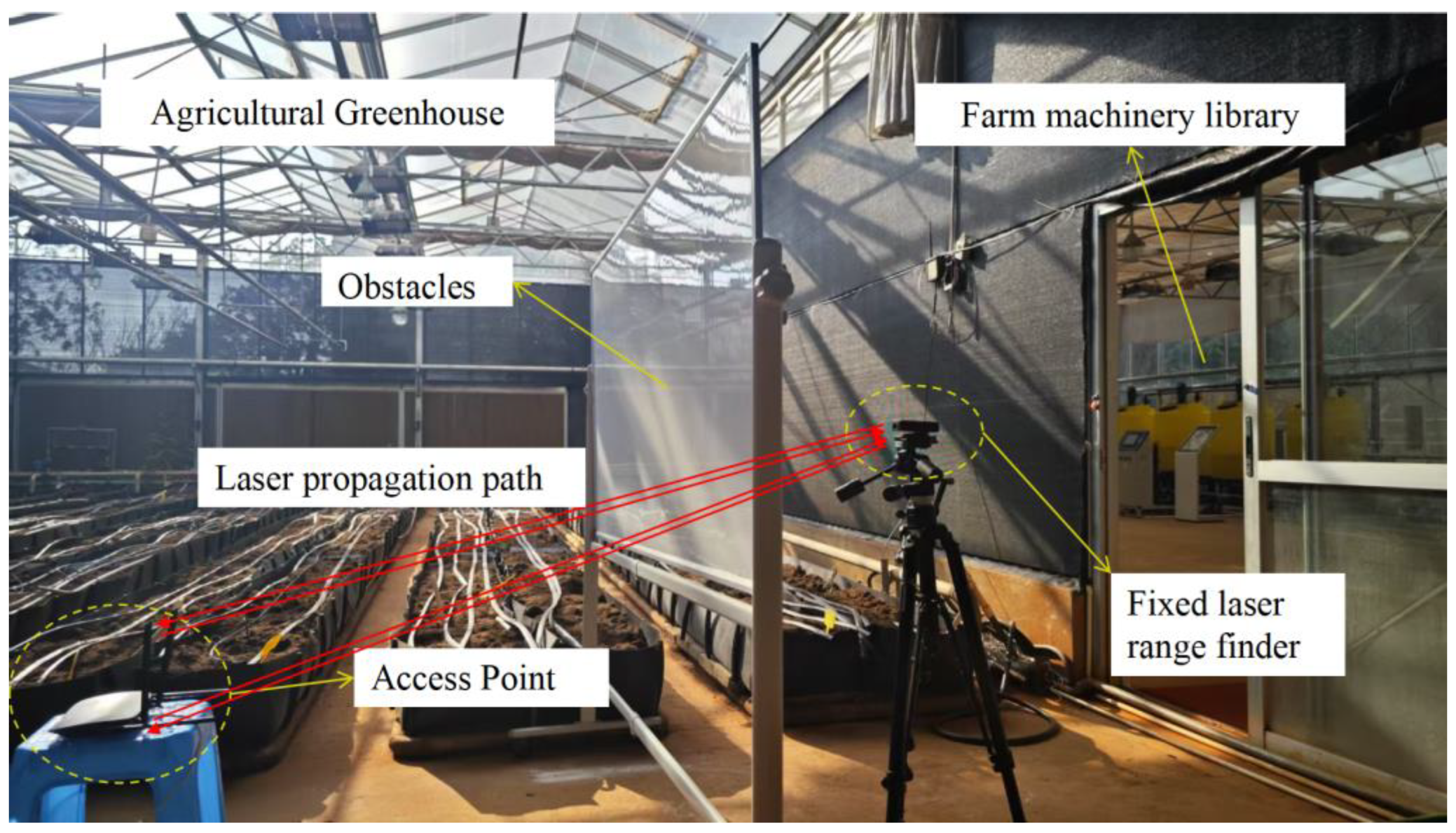
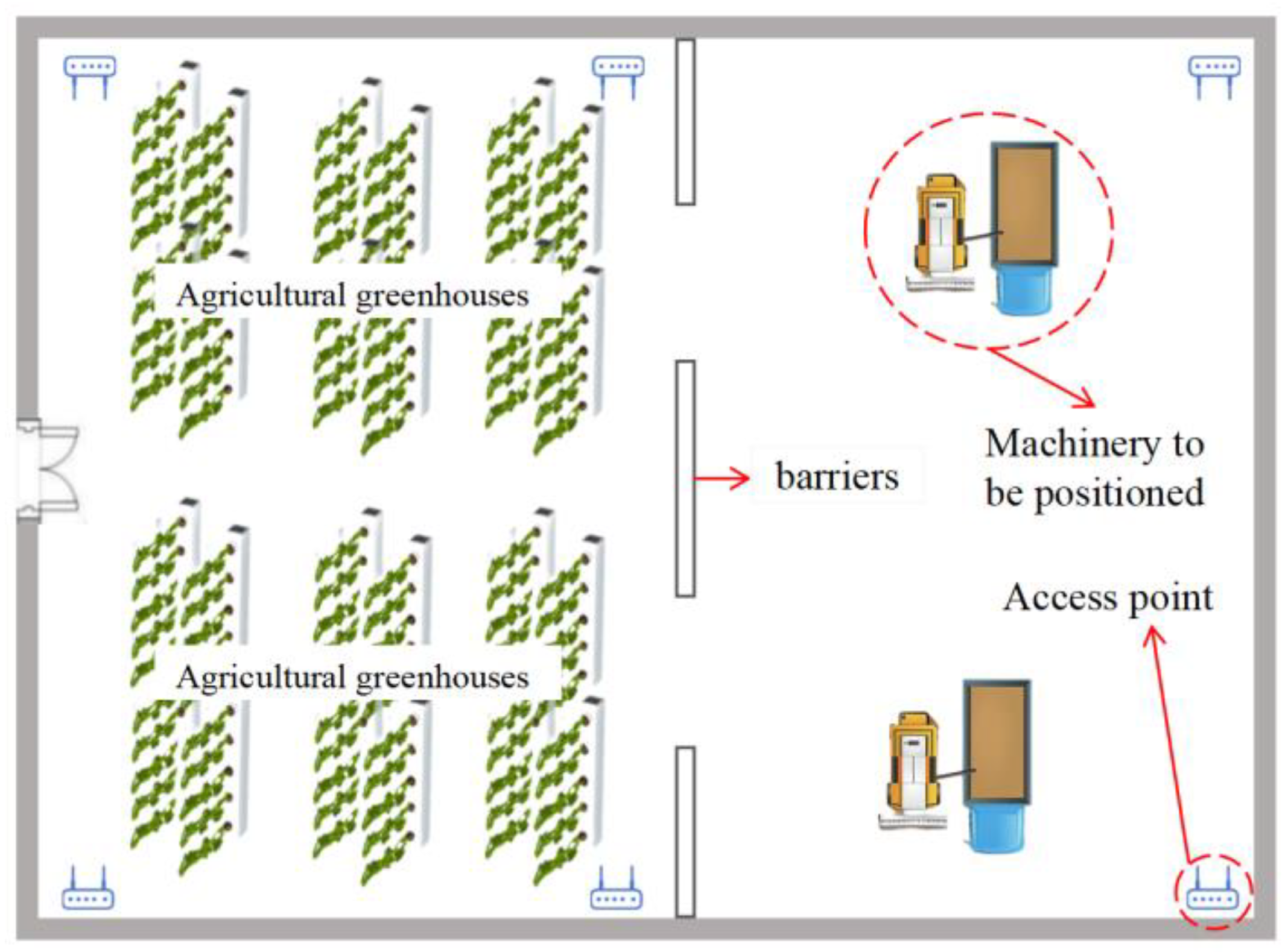
6.1. Test Environmental Setup

The RSSI values of the WI-FI signals used in this study were collected from the indoor smart agriculture greenhouse and machinery hangar at the College of Agriculture, Kunming University of Science and Technology. As shown in Figure 8, the environment was complex, containing multiple obstructions that affected the signal quality, the red arrows represent the path of laser propagation. The site comprised an agricultural planting area and an agricultural machinery hangar. The “TL-WDR5620 (manufactured by [TP-LINK], [Shenzhen City], [CHINA])” router was used to generate WI-FI signals, connected to a “Xiaomi 13 Pro” smartphone for communication. Signal strength was measured using the An-droid-based application “WI-FI Magic Box (manufactured by [RUIJIE NETWORKS], [Fujian Province], [CHINA])”. The distance between the smartphone and the router was determined using a “DLX-B2605 (manufactured by [DELIXI ELECTRIC], [Zhejiang Province], [CHINA])” laser distance meter mounted on a tripod to maintain consistent measurement angle and height, ensuring that its front end was horizontally aligned with the smartphone receiving the Wi-Fi signal. The signal transmission path between the router and the smartphone included various obstacles.

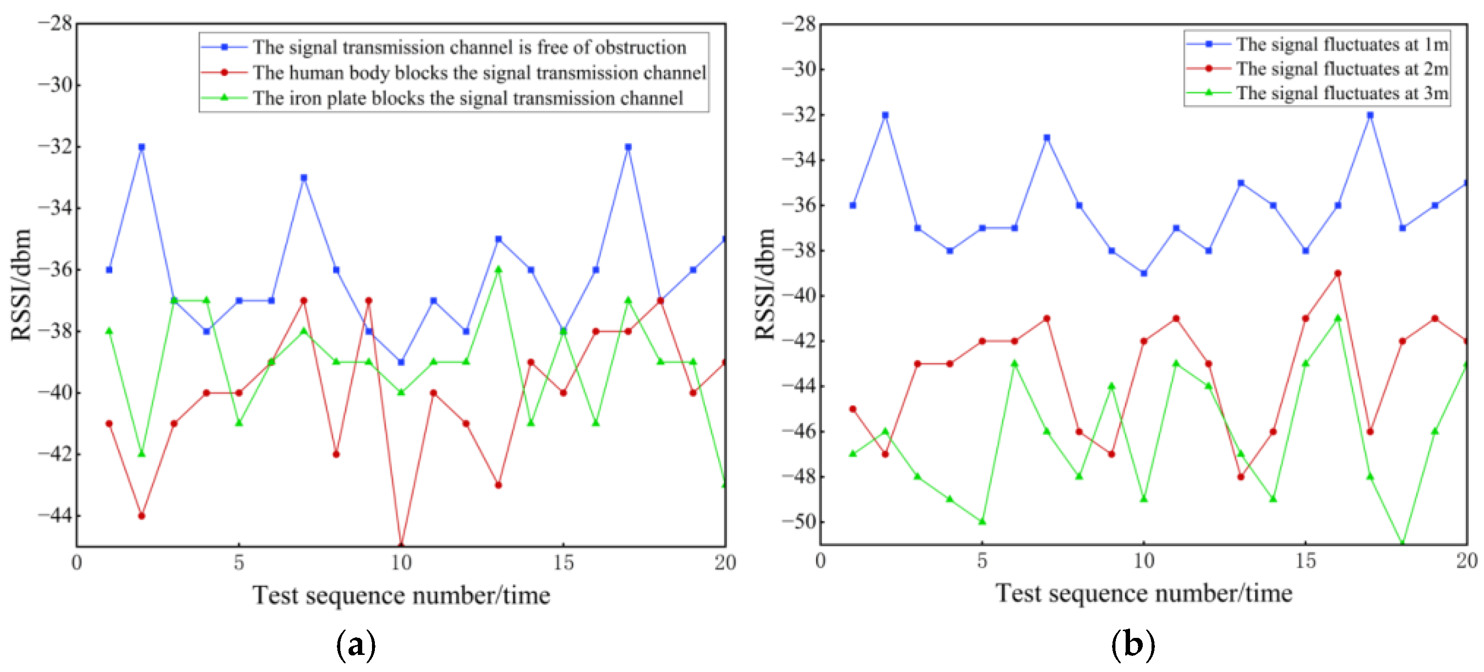
6.2. RSSI Signal Quality Analysis

The volatility of the RSSI signals in the laboratory environment was analyzed, as shown in Figure 8, using the following patterns:

(1) Unobstructed signal transmission: Signal strength variations were recorded for distances of 1 m, 2 m, and 3 m between the access point (AP) and the sampling device. Data were collected 20 times at 3 s intervals. The results are shown in Figure 9a, where it can be seen that a fluctuation range was 15.8% for a 1 m distance, 18.75% for a 2 m distance, and 15.6% for a 3 m distance;

(2) Obstructed signal transmission: At a 1-m distance between the AP and the mobile sampling device, three common indoor scenarios were considered: unobstructed signal transmission, signal transmission obstructed by a human body, and signal transmission obstructed by an iron plate. The variations in the RSSI signal strength are illustrated in Figure 9b, where a fluctuation range of 28.9% for different obstacles at the same distance of 1 m can be observed.

The experimental results indicated that the RSSI signals in agricultural greenhouses were susceptible to environmental changes and exhibited significant fluctuations, which severely affected the accuracy of the ranging algorithms. In addressing this problem, the proposed IBKA-BP positioning algorithm used the Kalman filtering and Min-Max normalization methods to process the collected sample data. These methods reduced noise interference caused by environmental factors and device errors, smoothing RSSI signal fluctuations by estimating system states and updating predictions. As a result, the algorithm’s positioning accuracy and robustness were improved.

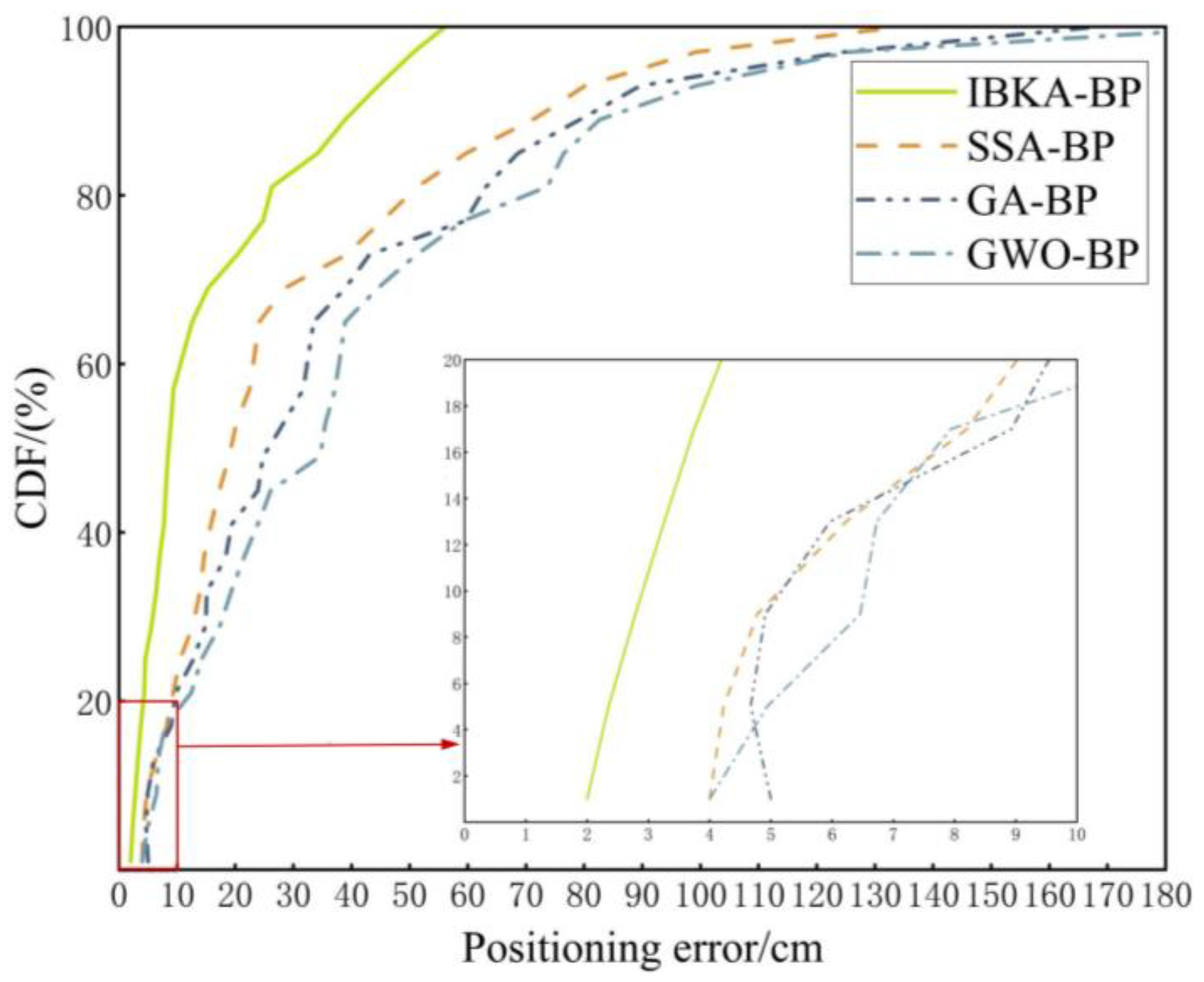
6.3. Localization Performance Analysis of Different Algorithms

In evaluating the localization performance of the proposed algorithm, this study conducted a simulation experiment using the MATLAB 2022a software in the simulation environment depicted in Figure 10. The simulated agricultural greenhouse covered a localization area with a size of 8 m × 10 m; the router placement and sampling distribution are shown in Figure 10. Six routers were positioned at the area’s corners and served as base stations. The sampling points were located at every 0.5 m, covering the range from 0.5 m to 9.5 m along both the x-axis and the y-axis. The RSSI signal strength and distance values collected from the laboratory were used as training samples for the model and location prediction, following the algorithm flowchart presented in Figure 7. The parameters included a path loss exponent $\eta$ of 2.02, an RSSI value A of −40 dBm at the reference distance of 1 m, a shadow fading standard deviation $\sigma$ of 3 dB, and a signal-to-noise ratio SNR of −30 dB. During data preprocessing, the Kalman filter parameters were selected as follows: state transition matrix A = 0.95, measurement matrix H = 1, process noise covariance Q = 0.01, and measurement noise covariance R = 0.1.

The cumulative distribution function (CDF) plots of localization errors of the tested algorithms are presented in Figure 11. The percentage of localization errors smaller than 15 cm for the IBKA-BP, SSA-BP, GA-BP, and GWO-BP algorithms were 68%, 40%, 32%, and 28%, and their median localization errors were 8.05 cm, 17.24 cm, 23.91 cm, and 26.15 cm, highlighting the superior accuracy of the IBKA-BP algorithm.

In evaluating the positioning accuracy of the proposed IBKA-BP ranging model, this study performed a comparative analysis with the SSA-BP, GA-BP, and GWO-BP algorithms. The RSSI signal strength and distance values were collected in the experimental environment (depicted in Figure 10) and used as training samples for the model, which was followed by the position prediction process. The model had four input layer nodes, four output layer nodes, and 10 hidden layer nodes. The population size and maximum iteration number were set to 40 and 100, respectively. All four algorithms were evaluated in identical simulated environments by randomly generating 100 nodes to be localized. The ME, STD, and RMSE values of 100 independent localization trials were statistically evaluated, as presented in

Table 1. Error results of different algorithms.

Algorithm	ME (cm)	SD (cm)	RMSE (cm)
IBKA-BP	16.34	16.32	22.87
Sparrow Search Algorithm— Backpropagation	33.67	33.35	46.19
Genetic Algorithm—Backpropagation	39.90	40.72	56.42
Grey Wolf Optimizer—Backpropagation	44.76	45.56	62.67

.

As shown in Table 1, the IBKA-BP algorithm exhibited noticeably smaller errors compared to the other algorithms. Particularly, the IBKA-BP algorithm achieved an ME of 16.34 cm, an STD of 16.32 cm, and an RMSE of 22.87 cm, outperforming the SSA-BP, GA-BP, and GWO-BP algorithms. The simulation results confirmed that the proposed algorithm could effectively use a base station selection strategy to identify the most suitable base stations for the current localization environment. Moreover, the integration of tent mapping expanded the range of effective solutions, enhancing global optimization capabilities. The lens imaging-based reverse learning strategy further improved the BP model’s feature extraction capabilities by simulating the lens imaging process. This approach could suppress unnecessary noise and capture the nonlinear relationships in RSSI signals more effectively than the other algorithms, achieving higher accuracy in indoor localization.

6.4. Comparison of Positioning Accuracy Under WI-FI Radio Frequency Interference

To evaluate the anti-interference performance of the proposed algorithm, we conducted comparative experiments with Whale Optimization Algorithm Optimized Backpropagation (WOA-BP), SSA-BP, GA-BP, and GWO-BP. To precisely control environmental variables (e.g., temperature, humidity, and static obstacles) and isolate interference effects from other RF sources, ensuring observed performance variations originated solely from the introduced WI-FI router interference, the laboratory environment shown in Figure 12 was selected. A “Xiaomi 4A” router served as the WI-FI signal interference source, with the WI-FI signal source for collecting RSSI signal strength positioned 1.5 m from the interference source. Experimental parameter settings remained consistent with previous configurations. The ME, STD, and RMSE values of positioning errors for different algorithms across 100 independent trials are presented in

Table 2. Error results of different algorithms under WI-FI interference.

Algorithm	ME (cm)	SD (cm)	RMSE (cm)
IBKA-BP	29.71	29.13	39.86
Sparrow Search Algorithm— Back Propagation	52.53	53.15	74.61
Genetic Algorithm—Back Propagation	61.05	61.93	85.56
Grey Wolf Optimizer—Back Propagation	69.75	71.27	96.37

.

Experimental results shown in Table 2 reveal that when a Wi-Fi signal served as a radio frequency interference source at a 1.5-m distance, the positioning accuracy of all four algorithms significantly decreased. Under these conditions, the IBKA-BP algorithm achieved a ME of 29.71 cm, a STD of 29.13 cm, and a RMSE of 39.86 cm, still outperforming the other three comparative algorithms. This demonstrates that the proposed IBKA-BP algorithm effectively suppressed signal fluctuations caused by Wi-Fi interference through Kalman filtering during the signal preprocessing stage, which dynamically estimated the true RSSI values. Furthermore, the IBKA Algorithm significantly optimized the global adaptability of neural network weights and thresholds, enabling high-precision positioning even in environments with radio frequency interference.

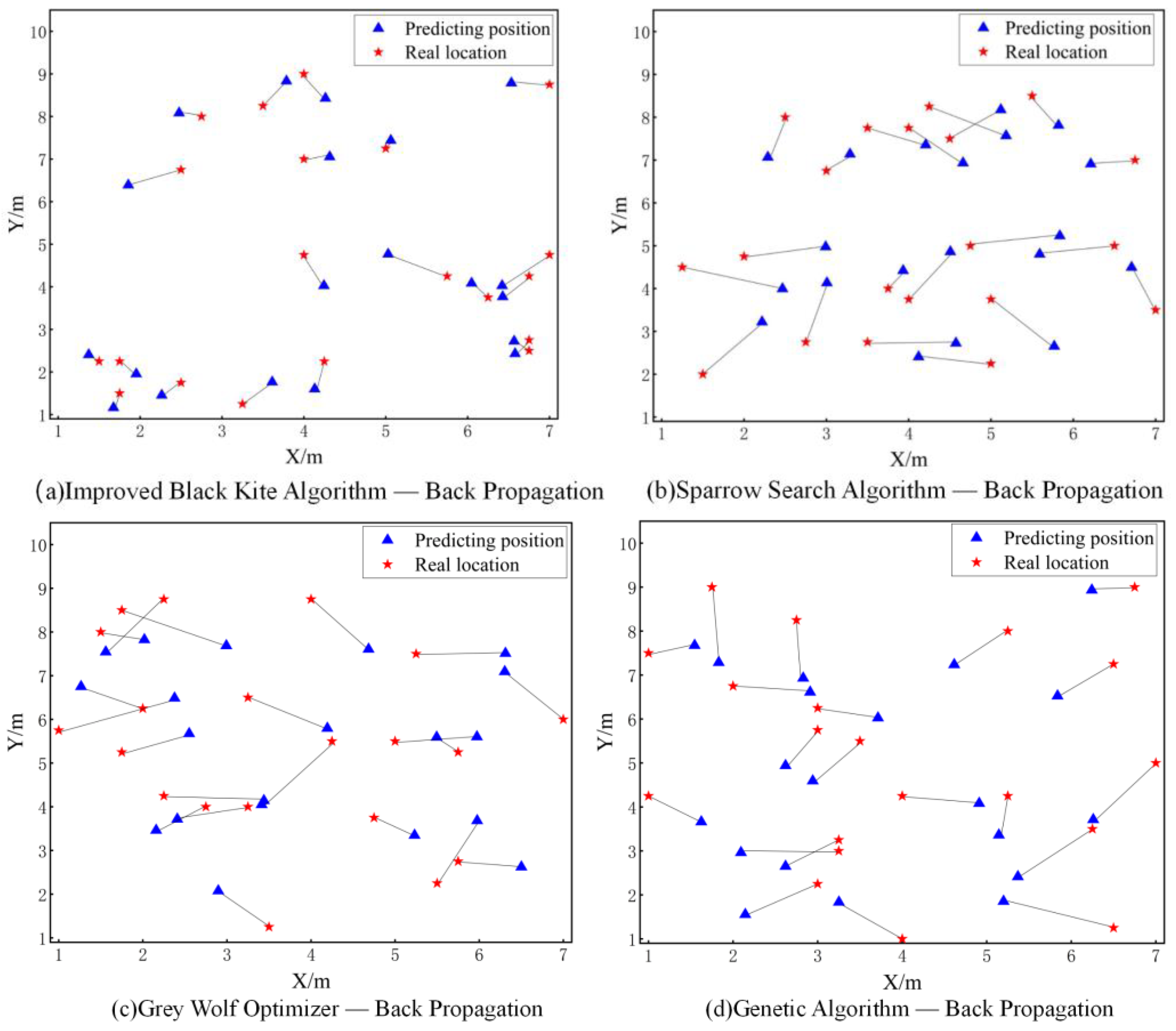
6.5. Positioning Result Comparison of Different Algorithms

Next, the RSSI signal strength and distance data were collected in the agricultural greenhouse planting area and the farm machinery storage and used as test samples. These samples were used for position prediction using four algorithms, namely the IBKA-BP, SSA-BP, GA-BP, and GWO-BP algorithms. To overcrowding the observations, 15 test points were randomly selected. The positioning results of the four algorithms are displayed in Figure 13, where the red pentagrams represent the true locations of the test points, and the blue triangles denote the predicted locations. The results indicated that among all algorithms, the proposed IBKA-BP algorithm achieved the predicted locations closest to the true positions, demonstrating superior positioning performance compared to the other algorithms.

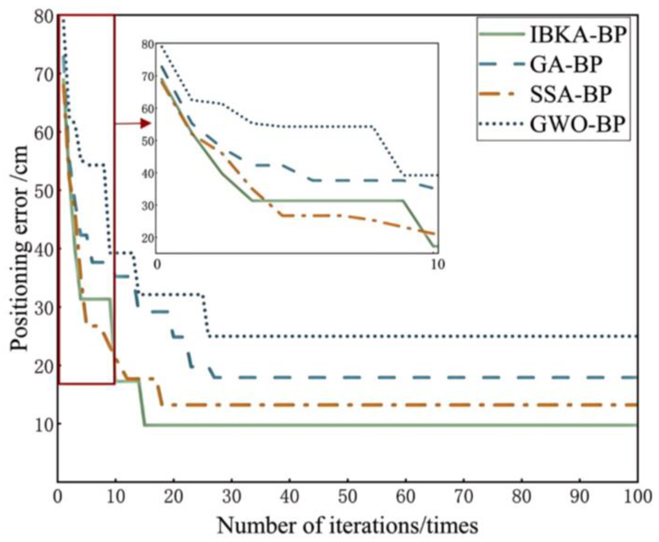
6.6. Algorithm Convergence Analysis

In validating the convergence capability of the proposed IBKA algorithm, this study conducted a comparative analysis using the neural network ranging models trained by different optimization algorithms. The optimization objective was to minimize the positioning error of the ranging model. The convergence status of the fitness values of different optimization algorithms is illustrated in Figure 14. In this experiment, the population size was set to 30, the number of iterations was 100, and identical parameter settings were used for all algorithms to ensure a fair comparison.

As shown in Figure 13, the IBKA-BP algorithm achieved the optimal fitness value within fewer iterations than the other algorithms. Its efficiency could be mostly attributed to the application of the tent mapping strategy, which generated complex and highly random sequences, aiding in the creation of diverse initial populations and effective parameter adjustments. This strategy prevented the algorithm from becoming trapped in local optima, thus reducing the number of iterations required to achieve optimal fitness. In addition, the implementation of the golden sine strategy, which combined the properties of the golden ratio and the sine function, enhanced the algorithm’s exploration and exploitation capabilities. This balanced approach enabled effective global and local searches, allowing the proposed algorithm to converge more precisely near the optimal solution. Consequently, the IBKA-BP algorithm demonstrated faster convergence and higher efficiency in achieving optimal fitness than the other algorithms.

6.7. Comparison with Recent Advancements in AI-Based Localization Field

Recent breakthroughs in the AI field have revolutionized positioning technologies, and deep learning-based indoor localization systems have demonstrated remarkable performance in the industrial Internet of Things (IoT), healthcare monitoring, and autonomous driving applications. Notably, Pu et al. [43] proposed a generative AI-RIS fusion localization framework and developed a variational autoencoder-convolutional neural network (VAE-CNN) model for noise reduction and signal feature extraction. By integrating sparse modeling and semi-tensor product theory, their approach could achieve superior positioning accuracy and computational efficiency compared to conventional methods. Yang et al. [44] addressed the challenge of inaccurate access point localization under a limited Wi-Fi beacon bandwidth of 20 MHz using an adaptive AI filter. Their methodology employed dynamic AP selection criteria with coarse-to-fine localization refinement, allowing for achieving a decimeter-level accuracy, which represented a significant advancement validated by rigorous experimentation. Meanwhile, Gao et al. [45] overcame the 6G digital twin localization limitations by adopting a seven-layer localization-oriented DT (LocDT) architecture. This innovation constructed high-precision fingerprint databases through environmental modeling and channel frequency polar coordinate imaging, enhanced by an SSI-Net model with device attention mechanisms. Their solution could effectively fuse the LOS and NLOS base station features in partial visibility scenarios, achieving unprecedented precision and real-time performance.

Despite the aforementioned advancements, systematic research on AI-driven localization for agricultural robots has still been scarce. Namely, the existing studies have predominantly focused on outdoor GNSS enhancement, leaving critical gaps in the AI-powered positioning solutions for controlled agricultural environments, such as greenhouses; this has yielded a bottleneck hindering precision cultivation and automated harvesting technologies. However, the proposed algorithm can address this shortcoming by combining a multi-strategy optimization framework and a base station screening mechanism, thus achieving exceptional positioning accuracy in complex scenarios. Particularly, its unique capability to correct signal distortion under NLOS interference caused by metal greenhouse frameworks is noteworthy and has a substantial engineering value for modern agricultural infrastructure.

Further, to systematically evaluate performance, this study conducted comparative analyses with three state-of-the-art AI-based localization methods in terms of three critical performance evaluation indicators: environmental adaptability, computational efficiency, and dynamic interference mitigation. The comprehensive comparison results are presented in

Table 3. The environmental adaptability comparison results.

Algorithm	Strengths	Limitations
IBKA-BP	1. Dynamic NLOS base station screening can adapt to multi-obstacle environments (e.g., metal greenhouse frameworks); 2. Kalman filtering can effectively suppress time-varying signal noise caused by temperature/humidity fluctuations	1. Algorithm performance degrades with sparse Wi-Fi base station deployment; 2. Algorithm lacks multi-band signal fusion capability
Reconfigurable intelligent surface-aided localization	1. Enhancing signal coverage requires pre-deployed reconfigurable intelligent surface (RIS) intelligent reflecting surfaces in single-AP scenarios; 2. Improves NLOS robustness through the VAE-CNN denoising	1. Expensive RIS hardware; 2. Limited scalability due to dependence on the RIS reflector quantity
AI-based filter	1. Adapts well to low-bandwidth signals (20 MHz) using dynamic AP selection criteria; 2. Adjust filtering thresholds based on known AP locations	1. Relies on prior AP position knowledge (complex calibration); 2. Neglects dynamic multipath interference effects
Localization-oriented digital twinnings	1. Seven-layer digital twin architecture models physical environments for partial LOS scenarios; 2. Channel frequency polar-coordinate (CFP) polar-coordinate imaging enhances channel fingerprint distinction.	1. Requires high-precision environmental modeling (high deployment complexity); 2. Dependent on the 6G network infrastructure (currently impractical)

,

Table 4. The computational efficiency comparison results.

Algorithm	Optimization Strategy	Computational Cost
IBKA-BP	1. Dynamic base station screening reduces modeling complexity. 2. Min-Max normalization accelerates gradient descent convergence.	Low (minimal hardware requirements)
Reconfigurable intelligent surface-aided localization	1. Semi-tensor product (STP) compresses sparse matrix dimensions. 2. Parallelized VAE-CNN feature extraction.	High (requires generative adversarial network (GAN) training with GPU acceleration)
AI-based filter	1. Progressive accuracy refinement reduces redundant computations. 2. Lightweight AI filter design.	Low (real-time AI-driven parameter filtering)
Localization-oriented digital twinnings	1. Hierarchical digital twin architecture enables phased optimization. 2. SSI-Net attention mechanism minimizes redundant calculations.	Extremely high (real-time environmental modeling + CFP image generation)

and

Table 5. The dynamic interference mitigation comparison results.

Algorithm	Advantages	Limitations
IBKA-BP	1. Can effectively suppress short-term signal fluctuations by using Kalman filtering and NLOS base station screening; 2. Maintains high positioning accuracy under interference	Lacks the multi-band interference coordination capability
Reconfigurable intelligent surface-aided localization	1. Compensates for the signal loss using the GAN-based data augmentation approach; 2. Dynamic RIS reflector configuration optimizes signal paths	Requires real-time RIS hardware control (high operational costs)
AI-based filter	Implements adaptive thresholding to filter anomalous parameters	A lack of a dedicated multipath effect suppression module
Localization-oriented digital twinnings	1. Digital twin-enabled interference prediction improves partial LOS scenarios; 2. Enhances positioning reliability through environmental modeling	Latency in dynamic model updates limits the real-time responsiveness

.

The proposed algorithm has three main advantages: robust anti-interference capability without the requirement for additional hardware support, high computational efficiency in real-time localization, and superior positioning accuracy in agricultural greenhouses characterized by dense obstacles and dynamic environmental fluctuations. In addition, in large-scale farms and greenhouse environments, a hybrid network can be established by deploying base stations at a high density in key areas (e.g., greenhouse entrances/exits and high-activity zones) and a lower density in peripheral regions. This approach can effectively reduce the total cost. However, in practical applications, agricultural robots are required to operate stably over extended periods in complex environments containing dust, extreme temperature, and humidity conditions. Therefore, sensors and base stations must possess anti-interference capabilities and low-power consumption features. Moreover, interference from overlapping frequency bands used by the Wi-Fi, Bluetooth, and agricultural machinery communication devices in agricultural scenarios, as well as potential communication interruptions caused by heavy rain or snow, must be addressed. Considering all the mentioned, the deployment of redundant signal networks is recommended to ensure the stable operation of positioning systems.

7. Conclusions

The main conclusions of this work can be summarized as follows:

(1) A base station identification algorithm is used to select the most suitable base station for positioning at a given location. The data collected from this base station are used for subsequent indoor localization. The experimental results show that the proposed frequency statistics-based base station identification method can effectively distinguish the NLOS base stations, improving positioning accuracy. Further, a multi-strategy fusion-based improved black kite optimization algorithm is developed by integrating the tent mapping method, the golden sine strategy, and the lens imaging reverse learning strategy. This enables the black kite algorithm to optimize the BP neural network by selecting more effective weights and thresholds, which significantly improves its performance;

(2) Kalman filtering is performed as a preprocessing step to reduce signal fluctuations and improve data stability. The IBKA-BP ranging model is developed to capture the nonlinear relationship between the signal strength and distance. The results of the comparative experiments conducted using the IBKA-BP, sparrow search algorithm-backpropagation, genetic algorithm-backpropagation, and grey wolf optimizer-backpropagation algorithms demonstrate that the proposed IBKA-BP algorithm can provide the most accurate predicted positions among all algorithms. In the positioning error analysis, the IBKA-BP algorithm achieves the lowest errors, with the ME, STD, and RMSE values of 16.34 cm, 16.32 cm, and 22.87 cm, respectively. Furthermore, 68% of IBKA-BP positioning errors are below 15 cm, the highest among the four algorithms; also, the proposed algorithm exhibits the fastest convergence among all algorithms, confirming its superior performance in complex indoor environments;

(3) Further, after integrating the proposed algorithm with the existing farm management systems, the IBKA-BP positioning data can serve as input for farm management systems and can be combined with machine-learning models to predict crop requirements. For instance, in precision fertilization, a system can dynamically adjust fertilizer application rates based on a robot’s position and soil data. In pest and disease monitoring, a robot’s positioning data, combined with multispectral images, can precisely mark infected areas, thus guiding targeted pesticide application. Moreover, integrating positioning algorithms with farm management systems can help achieve dual goals of resource efficiency improvement and labor cost reduction;

(4) However, the proposed algorithm has a few limitations in practical applications. First, its positioning performance greatly depends on the planning and deploying processes of Wi-Fi base stations. Namely, in agricultural scenarios with irregular terrain or dynamic vegetation changes, achieving an optimal base station layout is highly challenging. In addition, an insufficient deployment can lead to signal attenuation and coverage blind spots, whereas redundant setups can significantly increase infrastructure costs. Second, the proposed algorithm’s sole reliance on the RSSI measurements limits its adaptability to mission-critical scenarios. Finally, the lack of multi-sensor fusion with inertial navigation units, LiDAR, or vision systems makes the proposed algorithm susceptible to temporary signal blockages caused by moving agricultural machinery or dense crop canopies.

In addressing the above-mentioned limitations, future work could focus on enhancing the proposed algorithm by using LiDAR or millimeter-wave radar data to construct real-time dynamic obstacle maps. These maps could help to accurately identify and mitigate the impact of dynamic obstacles in complex environments. In addition, a time-series prediction model could be incorporated to dynamically update the NLOS base station filtering strategy. This integration could improve the adaptability and robustness of the positioning system, enabling more reliable performance in diverse and challenging agricultural environments.

References

1. Nijak, M.; Skrzypczyński, P.; Ćwian, K.; Zawada, M.; Szymczyk, S.; Wojciechowski, J. On the Importance of Precise Positioning in Robotised Agriculture. Remote Sens. 2024, 16, 985. [Google Scholar] [CrossRef]
2. Qu, J.; Qiu, Z.; Li, L.; Guo, K.; Li, D. Map Construction and Positioning Method for LiDAR SLAM-Based Navigation of an Agricultural Field Inspection Robot. Agronomy 2024, 14, 2365. [Google Scholar] [CrossRef]
3. Yang, Q.; Du, X.; Wang, Z.; Meng, Z.; Ma, Z.; Zhang, Q. A review of core agricultural robot technologies for crop productions. Comput Electron. Agric. 2023, 206, 107701. [Google Scholar] [CrossRef]
4. Wang, R.; Chen, L.; Huang, Z.; Zhang, W.; Wu, S. A Review on the High-Efficiency Detection and Precision Positioning Technology Application of Agricultural Robots. Processes. 2024, 12, 1833. [Google Scholar] [CrossRef]
5. Nimma, D.; Dhanke, J.A.; Murthy, G.; Khandekar, S.D.; Hymavathi, J.; Jangir, P.; Singh, M. Optimization of Crop Yields in Sustainable Agriculture: Application of Big Data Analytics and Artificial Intelligence. Remote. Sens. Earth Syst. Sci. 2025, 1–12. [Google Scholar] [CrossRef]
6. Lv, P.; Wang, B.; Cheng, F.; Xue, J. Multi-objective association detection of farmland obstacles based on information fusion of millimeter wave radar and camera. Sensors. 2022, 23, 230. [Google Scholar] [CrossRef]
7. Nie, S.; Lunar, M.M.; Bai, G.; Ge, Y.; Pitla, S.; Koksal, C.E.; Vuran, M.C. mmWave on a farm: Channel modeling for wireless agricultural networks at broadband millimeter-wave frequency. In Proceedings of the 2022 19th Annual IEEE International Conference on Sensing, Communication, and Networking (SECON), Stockholm, Sweden, 25 October 2022. [Google Scholar]
8. Ge, H.; Li, B.; Jia, S.; Nie, L.; Wu, T.; Yang, Z.; Shang, J.; Zheng, Y.; Ge, M. LEO enhanced global navigation satellite system (LeGNSS): Progress, opportunities, and challenges. GSIS 2022, 25, 1–13. [Google Scholar] [CrossRef]
9. Yao, Z.; Zhao, C.; Zhang, T. Agricultural machinery automatic navigation technology. iScience 2024, 27, 108714. [Google Scholar] [CrossRef]
10. Xie, K.; Zhang, Z.; Zhu, S. Enhanced Agricultural Vehicle Positioning through Ultra-Wideband-Assisted Global Navigation Satellite Systems and Bayesian Integration Techniques. Agriculture 2024, 14, 1396. [Google Scholar] [CrossRef]
11. Shang, S.; Wang, L. Overview of WiFi fingerprinting-based indoor positioning. IET Commun. 2022, 16, 725–733. [Google Scholar] [CrossRef]
12. Lin, Y.; Yu, K.; Zhu, F.; Bu, J.; Dua, X. The state of the art of deep learning-based Wi-Fi indoor positioning: A review. IEEE Sens. J. 2024, 24, 27076–27098. [Google Scholar] [CrossRef]
13. Zhang, X.; Sun, W.; Zheng, J.; Lin, A.; Liu, J.; Ge, S.S. Wi-fi-based indoor localization with interval random analysis and improved particle swarm optimization. IEEE Trans. Mob. Comput. 2024, 23, 9120–9134. [Google Scholar] [CrossRef]
14. Zheng, J.; Li, K.; Zhang, X. Wi-Fi fingerprint-based indoor localization method via standard particle swarm optimization. Sensors 2022, 22, 5051. [Google Scholar] [CrossRef] [PubMed]
15. Huo, Y.; Puspitaningayu, P.; Funabiki, N.; Hamazaki, K.; Kuribayashi, M.; Kojima, K. A proposal of the fingerprint optimization method for the fingerprint-based indoor localization system with IEEE 802.15. 4 devices. Information 2022, 13, 211. [Google Scholar] [CrossRef]
16. Cao, H.; Wang, Y.; Bi, J.; Zhang, Y.; Yao, G.; Feng, Y.; Si, M. LOS compensation and trusted NLOS recognition assisted WiFi RTT indoor positioning algorithm. Expert Syst. Appl. 2024, 243, 122867. [Google Scholar] [CrossRef]
17. Hou, C.; Liu, W.; Tang, H.; Cheng, J.; Zhu, X.; Chen, M.; Gao, C.; Wei, G. Non-Line-of-Sight Positioning Method for Ultra-Wideband/Miniature Inertial Measurement Unit Integrated System Based on Extended Kalman Particle Filter. Drones 2024, 8, 372. [Google Scholar] [CrossRef]
18. Kong, Q. NLOS identification for UWB positioning based on IDBO and convolutional neural networks. IEEE Access 2023, 11, 144705–144721. [Google Scholar] [CrossRef]
19. Ahirwal, S.; Singh, J. A Review of Range-based RSSI Algorithms for Indoor Wireless Sensor Network Localization. Int. J. Adv. Comput. Technol. 2023, 12, 7–12. [Google Scholar]
20. Arigye, W.; Pu, Q.; Zhou, M.; Khalid, W.; Tahir, M.J. RSSI fingerprint height based empirical model prediction for smart indoor localization. Sensors 2022, 22, 9054. [Google Scholar] [CrossRef]
21. Du, J.; Yuan, C.; Yue, M.; Ma, T. A novel localization algorithm based on RSSI and multilateration for indoor environments. Electronics 2022, 11, 289. [Google Scholar] [CrossRef]
22. Liu, T.; Ji, J.; Pan, D.; Zhao, L.; Li, M. Localization method for agricultural robots based on fusion of LiDAR and IMU. Smart Agric. 2024, 6, 94. [Google Scholar]
23. Zhao, L.; Han, Z.; Zhang, F. Research on Stereo Location in Visible Light Room Based on Neural Network. Chin. J. Lasers 2021, 48, 706004. [Google Scholar]
24. Tian, Y.; Lian, Z.; Wang, P.; Wang, M.; Yue, Z.; Chai, H. Application of a long short-term memory neural network algorithm fused with Kalman filter in UWB indoor positioning. Sci. Rep. 2024, 14, 1925. [Google Scholar] [CrossRef] [PubMed]
25. Gui, L.; Yang, M.; Yu, H.; Li, J.; Shu, F.; Xiao, F. A Cramer-Rao lower bound of CSI-based indoor localization. IEEE Trans. Veh. Technol. 2017, 67, 2814–2818. [Google Scholar] [CrossRef]
26. Bi, J.; Wang, Y.; Ning, Y. Indoor rang-based positioning method considering geometry optimization of BLE beacons. J. China Univ. Min. Technol. 2021, 50, 411–416. [Google Scholar]
27. Rodriguez, A.; Laio, A. Clustering by fast search and find of density peaks. Science 2014, 344, 1492–1496. [Google Scholar] [CrossRef]
28. Li, G.; Geng, E.; Ye, Z.; Xu, Y.; Lin, J.; Pang, Y. Indoor positioning algorithm based on the improved RSSI distance model. Sensors 2018, 18, 2820. [Google Scholar] [CrossRef]
29. Nosrati, L.; Fazel, M.S.; Ghavami, M. Improving indoor localization using mobile UWB sensor and deep neural networks. IEEE Access 2022, 10, 20420–20431. [Google Scholar] [CrossRef]
30. Khodarahmi, M.; Maihami, V. A review on Kalman filter models. Arch. Comput. Methods Eng. 2023, 30, 727–747. [Google Scholar] [CrossRef]
31. Feng, D.; Wang, C.; He, C.; Zhuang, Y.; Xia, X.-G. Kalman-filter-based integration of IMU and UWB for high-accuracy indoor positioning and navigation. IEEE Internet Things J. 2020, 7, 3133–3146. [Google Scholar] [CrossRef]
32. Xie, Y.; Jiang, L. RSSI Indoor Positioning Algorithm Based on Kalman Filtering. In Proceedings of the 2024 5th International Conference on Electronic Communication and Artificial Intelligence (ICECAI), Shenzhen, China, 24 September 2024. [Google Scholar]
33. Shantal, M.; Othman, Z.; Bakar, A.A. A novel approach for data feature weighting using correlation coefficients and min–max normalization. Symmetry 2023, 15, 2185. [Google Scholar] [CrossRef]
34. Henderi, H.; Wahyuningsih, T.; Rahwanto, E. Comparison of Min-Max normalization and Z-Score Normalization in the K-nearest neighbor (kNN) Algorithm to Test the Accuracy of Types of Breast Cancer. Int. J. Inform. Inf. Syst. 2021, 4, 13–20. [Google Scholar] [CrossRef]
35. Mu, C.; Qiu, B.; Liu, X. A new method for figuring the number of hidden layer nodes in BP algorithm. Int. J. Recent Innov. Trends Comput. Commun. 2017, 5, 101–114. [Google Scholar]
36. Tian, Y.; Su, D.; Lauria, S.; Liu, X. Recent advances on loss functions in deep learning for computer vision. Neurocomputing 2022, 497, 129–158. [Google Scholar] [CrossRef]
37. Wang, J.; Wang, W.; Hu, X.; Qiu, L.; Zang, H. Black-winged kite algorithm: A nature-inspired meta-heuristic for solving benchmark functions and engineering problems. Artif. Intell. Rev. 2024, 57, 1–53. [Google Scholar] [CrossRef]
38. Choi, T.J.; Togelius, J.; Cheong, Y. Advanced Cauchy mutation for differential evolution in numerical optimization. IEEE Access 2020, 8, 8720–8734. [Google Scholar] [CrossRef]
39. Zhang, X.; Wang, S. Firefly search algorithm based on leader strategy. Eng. Appl. Artif. Intell. 2023, 123, 106328. [Google Scholar] [CrossRef]
40. Su, Y.; Wang, S. Adaptive Hybrid Strategy Sparrow Search Algorithm. Comput. Eng. Appl. 2023, 59, 75–85. [Google Scholar]
41. Dexin, Y.; Linna, Z.; Damin, Z. Harris hawks optimization based on chaotic lens imaging learning and its application. Chin. J. Sens. Actuators 2021, 34, 1463–1474. [Google Scholar]
42. Liu, C.; He, Q. Golden Sine Chimp Optimization Algorithm Integrating Multiple Strategies. Acta Autom. Sin. 2023, 49, 2360–2373. [Google Scholar]
43. Pu, Q.; Yu, W.; Lan, X.; Zhou, M.; Yang, X. A Novel RIS-Aided Indoor Localization in Single Access Point Scenarios via Generative AI. IEEE Internet Things J. 2025. [Google Scholar] [CrossRef]
44. Yang, C.; Shih, W.; Wen, C.; Tsai, S.; Yuen, C. Enhancing WiFi access point localization with AI-based filtering. IEEE Commun. Letters 2024, 28, 1332–1336. [Google Scholar] [CrossRef]
45. Gao, K.; Wang, H.; Lv, H.; Liu, W. Localization-oriented digital twinning in 6G: A new indoor-positioning paradigm and proof-of-concept. IEEE Trans. Wirel. Commun. 2024, 23, 10473–10486. [Google Scholar] [CrossRef]
Figure 1. The flowchart of the BP neural network ranging process.
Agriculture 15 00901 g001
Figure 2. The clustering distribution diagram of positioning results.
Agriculture 15 00901 g002
Figure 3. The simulation environment layout diagram.
Agriculture 15 00901 g003
Figure 4. The simulation results of reliable base stations.
Agriculture 15 00901 g004
Figure 5. The BP neural network structure.
Agriculture 15 00901 g005
Figure 6. The lens imaging opposition-based learning strategy diagram.
Agriculture 15 00901 g006
Figure 7. The process flowchart of the RSSI ranging algorithm based on the IBKA-BP neural network.
Agriculture 15 00901 g007
Figure 8. Photo of the signal acquisition environment.
Agriculture 15 00901 g008
Figure 9. Results of signal propagation with different obstacles and distances.
Agriculture 15 00901 g009
Figure 10. The simulated diagram of the positioning environment simulation.
Agriculture 15 00901 g010
Figure 11. The CDF curves of the localization errors of different algorithms.
Agriculture 15 00901 g011
Figure 12. Localization experiment based on WI-FI Radio Frequency interference.
Agriculture 15 00901 g012
Figure 13. The distribution plots of the true and predicted positions for different algorithms.
Agriculture 15 00901 g013
Figure 14. The convergence performance comparison of different algorithms.
Agriculture 15 00901 g014