Abstract
This research focuses on developing an intelligent irrigation solution for agricultural systems utilising solar photovoltaic-thermal (PVT) energy applications. This solution integrates PVT applications, prediction, modelling and forecasting as well as plants’ physiological characteristics. The primary objective is to enhance water management and irrigation efficiency through innovative digital techniques tailored to different climate zones. In the initial phase, the performance of PVT solutions was evaluated using ANSYS Fluent software R19.2, revealing that scaled PVT systems offer optimal efficiency for PV systems, thereby optimising electrical production. Subsequently, a comprehensive approach combining integral feature selection (IFS) with machine learning (ML) and deep learning (DL) models was applied for reference evapotranspiration (ETo) prediction and water needs forecasting. Through this process, 301 optimal combinations of predictors and best-performing linear models for ETo prediction were identified. Achieving R2 values exceeding 0.97, alongside minimal indicators of dispersion, the results indicate the effectiveness and accuracy of the elaborated models in predicting the ETo. In addition, by employing a hybrid deep learning approach, 28 best models were developed for forecasting the next periods of ETo. Finally, an interface application was developed to house the identified models for predicting and forecasting the optimal water quantity required for specific plant or crop irrigation. This application serves as a user-friendly platform where users can input relevant predictors and obtain accurate predictions and forecasts based on the established models.
1. Introduction
As per the United Nations Environment Program’s (UNEP) annual report in 2000 [1], freshwater scarcity has been identified as the second most significant environmental challenge of the 21st century by scientists and political leaders. The demand for water is not only linked to ensuring access to drinking water for the population but also plays a critical role in supporting agriculture, tourism, and various industrial and agro-food sectors [2,3]. Consequently, water resources are central to systems of interaction that experience mounting pressures and conflicts among users.
Global climate trends have shown significant deviations from historical norms in recent years, including increased solar radiation intensity, elevated temperatures, and reduced precipitation levels. These changes contribute to various environmental challenges, such as droughts, climate change, floods, and the emergence or exacerbation of health risks. While some of these impacts are natural, a considerable portion can be attributed to human activities, particularly the extensive use of non-renewable energy sources over the past two centuries [4]. Furthermore, projections indicate that the global average air temperature will continue to rise in the coming decades due to increased anthropogenic CO2 emissions [5]. This ongoing warming is expected to disrupt both regional and global hydrological cycles, leading to alterations in precipitation patterns and increased water-related stress [6,7].
The Mediterranean region (including Morocco) is considered a global “hot point” regarding climate variability and change. According to forecasts made by the MAGICC model [8], it has been concluded that warming in the southern Mediterranean region is estimated to be at 3 °C by 2050 and 5 °C by 2100, while precipitation will decrease from 10 to 30% by 2050 and from 20 to 50% by 2100. These changes should put additional pressure on water management and, therefore, on agricultural production. Several studies [2,9,10,11] have deduced that regions with low and irregular productivity levels will be the ones most affected by the damage of climate change. A warming of 2 °C could lead to a permanent reduction of 4–5% of the annual per capita incomes in Africa and South Asia [12].
The impact of climate change will also affect the quantity and variability of water supplies [13,14] because changes in mean temperatures, even small ones, imply an increase in the frequency of extreme climatic conditions, namely drought and floods [15]. The increase in temperatures, the decrease in precipitation, and the increase in its variability imply a delay and a reduction in growth periods, as well as an acceleration of soil degradation and the loss of productive land [16]. These changes are expected to put additional pressure on agricultural production, although increasing atmospheric CO2 concentrations could potentially improve the photosynthesis process by up to 30% [17].
At the same time, the issues of greenhouse gas (GHG) emissions and the depletion of fossil fuels are ending conventional agricultural practices. With the infiltration of renewable technologies, the agriculture sector aims to feed the growing population in a more sustainable manner. Considering all the renewable energy sources, solar energy is among the most adaptable sources for farm applications. Over the years, solar PVT energy applications have been employed to supply the required power for various agricultural applications, including water pumping and irrigation, saltwater desalination, crop drying, and greenhouse cultivation [18]. However, emerging PV technology over water bodies through floating solar panels can resolve the challenge of substantial land requirements and additionally lead to operation of the panels at low temperatures, improving the energy generation efficiency and insulating water bodies to account for a reduction in evaporation loss [19].
Evapotranspiration (ET) serves as a fundamental link between the water needs of plants and the surrounding environment, playing a pivotal role in the growth, development, and survival of agricultural crops [20]. Understanding the intricate connection between ET and plant water needs is essential for optimising irrigation practices, conserving water resources, and enhancing agricultural sustainability. Water resource management requires more investigation in response to ET partitioning and water use efficiency [21].
ET directly reflects the combined effects of climatic factors, soil properties, and vegetation characteristics on water loss from the soil-plant-atmosphere continuum. It represents the total amount of water vapour transferred from the land surface to the atmosphere, integrating the influence of solar radiation, temperature, humidity, wind speed, and vegetation cover on water fluxes [22]. In agricultural settings, where water availability is often a limiting factor for crop growth, accurately estimating ET provides valuable insights into the timing and quantity of irrigation required to meet the water demands of crops [23]. ET is generally obtained by ground-based observations and model simulations. Compared with these models, machine learning (ML) and deep learning (DL) methods can directly, through prediction or forecasting, estimate ET from the provided data [24]. ML and DL models facilitate real-time ET forecasting and decision support systems for agricultural water management. By leveraging vast amounts of data from various sources, including meteorological observations, satellite imagery, soil moisture measurements, and vegetation indices, ML and DL models can provide accurate and timely predictions and forecasting of ET at different spatial and temporal scales [25].
Numerous ML-based and DL methods have been explored in the literature to approximate real ET values under varying climate conditions and crop characteristics. The authors of [26] suggested a combination forecasting model for estimating directly expected irrigation water. The authors of [27] employed measured ET as a predictor variable to facilitate land surface temperature (LST) modelling and forecasting. The authors of [23] employed a combination of decomposition techniques, feature selection methods, and ML approaches, including filter-based empirical mode decomposition (TVF-EMD), the tree-Boruta feature selection algorithm, a bidirectional recurrent neural network (Bi-RNN), a multilayer perceptron neural network (MLP), random forests (RFs), and extreme gradient boosting (XGBoost), are used to forecast weekly evapotranspiration. Their findings, with R2 values ranging between 0.87 and 0.92, emphasised the superiority of the TVF-BiRNN model in weekly ET prediction. In [25], the performance of random forest (RF) and long short-term memory (LSTM) neural networks was compared in calculating and forecasting the daily ET for three crops. Their results, with R2 values ranging from 0.5 to 0.7, indicated low performance accuracy. The authors of [28] proposed an XGBoost model to predict daily weather variables and subsequent ET at 51 weather stations across China. They reported R2 values between 0.56 and 0.85 for ET predictions. The authors of [29] introduced novel hybrid ML approaches for reference evapotranspiration (ETo) forecasting, utilising a multilayer perceptron-random forest (MLP-RF) stacked model and XNV. Their method achieved forecasting of ET 60 days ahead, with high-performance accuracy assessed by the Kling–Gupta (KGE) efficiency and mean absolute percentage error (MAPE), yielding values of 0.98 and 8.356%, respectively. The authors of [30] forecasted future reference evapotranspiration (ETO) values using a recurrent LSTM neural network optimised by the Coronavirus Optimization Algorithm. They reported an average R2 value of 0.7194. The authors of [31] conducted a comparative study of 10 ML methods for predicting evapotranspiration across large surfaces, where neural networks demonstrated the most favourable outcomes, with R2 values ranging between 0.69 and 0.73. The authors of [32] found the N-BEATS model to be the top-performing model for ETo time series forecasting among a set of statistical, ML, and DL models, with an R2 value close to one. The authors of [33] assessed LSTM and nonlinear autoregressive network with exogenous inputs (NARX) models for short-term (1–7 days ahead) actual ET prediction, reporting R2 values in the range of 0.82–0.91 for both models.
In this context, accurate prediction and monitoring of ET are crucial in guiding decision-making processes related to irrigation scheduling, water resource management, and crop yield optimisation. By integrating advanced modelling techniques, remote sensing technologies, and on-site measurements, researchers and practitioners can enhance our understanding of the complex interactions between ET and plant water needs. Through interdisciplinary approaches that bridge the gap between hydrology, agronomy, and climatology, we can develop innovative solutions to address the challenges of water scarcity, climate variability, and food security facing agricultural systems worldwide [34].
In recent years, growing attention has been directed toward integrated resource management frameworks that address the interconnections between water, energy, and food systems, particularly in the context of sustainable agriculture and irrigation [35]. Water-energy microgrids have emerged as localised, decentralised systems that combine renewable energy sources (e.g., photovoltaic or photovoltaic-thermal systems) with advanced water distribution technologies to optimise energy use and water delivery for agricultural applications. These microgrids enhance system resilience, reduce dependence on fossil fuels, and support precision irrigation strategies in off-grid or resource-constrained environments.
The water-energy-food (WEF) nexus also provides a holistic perspective for managing competing demands and interdependencies among essential resources. Nexus-based management systems aim to improve efficiency, sustainability, and policy coordination across sectors, particularly in regions vulnerable to climate change and resource scarcity. By aligning irrigation technologies with energy-efficient and environmentally conscious practices, WEF-based approaches contribute to long-term agricultural productivity and ecosystem preservation [36,37].
The present study builds on this paradigm by integrating machine and deep learning-based forecasting models with photovoltaic-thermal systems to support intelligent irrigation decisions, positioning our work within the broader landscape of smart water-energy management for sustainable agriculture.
In this study, a model for intelligent irrigation with PVT energy will be elaborated upon and proposed for the first time. When the literature was examined, no study was found for intelligent irrigation systems with PVT energy. Within this research, we will combine top-performing modelling, predicting, and forecasting techniques with PVT applications to deliver precise irrigation water estimates for sustainable agriculture. In the initial stage, we evaluated 13 common ML models to predict ETo, considering variables such as precipitation (P), temperature (T), relative humidity (RH), solar irradiance (H), wind speed (Ws), and wind direction (Wd). The top-performing ML model from this stage was combined with an integral feature selection (IFS) method to determine the most effective combinations of predictors for ETo predictions. Subsequently, in the second stage, we employed a Deep NARMAX model to identify optimal formulas for forecasting future ETo periods. By leveraging these two stages and utilising a specific equation, we accurately predicted and forecasted the quantity and quality of water required to irrigate specific plants or crops across diverse weather conditions. Concurrently, we conducted simulations and assessments of various configurations for PVT systems using Ansys Fluent. Through this process, we identified the most efficient configuration and determined the PVT delivered temperature under different climatic conditions. Finally, we developed an interface application using GUIDE MATLAB 2023a to integrate the identified models for predicting and forecasting the optimal water quantity and quality needed to irrigate specific plants or crops. This user-friendly platform allows users to input relevant predictors and obtain precise predictions and forecasts based on the established models.
The rest of the sections of this paper can be ordered as follows: Material and Methods, including data description, the locations considered, the model evaluation criteria, the PVT solution, the ML and DL models, the IFS approach, and the research methodology are summarized in Section 2. The results and discussions are given in Section 3, while the conclusions are listed in Section 4.
2. Material and Methods
2.1. Data and Statistical Analysis
2.1.1. Local Weather Information
The research was conducted using data sourced from locally implemented stations across 11 sites in Morocco. These locations experience a temperate climate characterised by long, hot summers and short, mild winters. The variables provided by each station include the ETo (mm), P (mm), T (MIN, AVR, and MAX in °C), RH (MIN, AVR, and MAX as percentages), H (kWh/m2), wind speed Ws (km/h), and wind direction Wd (degrees). Table 1 summarises the average values for each variable, along with information regarding the measurement period and geographical coordinates of each site. Table 2 summarises the predictor variables employed for predicting and forecasting ETO.

Table 1.
The chosen locations, corresponding periods, and average values for the provided data.
Table 2.
The variables employed in this work: inputs and output variables.
Figure 1 illustrates the level of correlation among all the analysed variables, including both the predictors and the output variable. A notable strong correlation was evident between ETo and H, followed by Tmax and Tmoy (average temperature). A less-strong correlation was observed with Tmin, while a negative moderate correlation was indicated by the RH. However, the other variables showed no significant correlation with ETo.
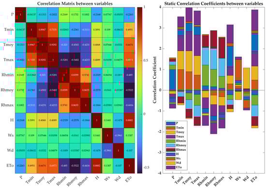
Figure 1.
Correlation between all examined variables.
2.1.2. Evapotranspiration and Water Need Computing
Crop water requirements are determined based on the maximum evapotranspiration estimated from the ETo. The water needs for a particular crop can be calculated as a function of evapotranspiration ETc, obtained by multiplying the ETo by a specific coefficient (Kc) corresponding to the crop type and its growth stage, as expressed in Equation (1):
For a given condition, the crop water requirements can be expressed as follows:
where Bn is the crop’s net water requirement; DS is the change in soil moisture (mm); and PE is the effective precipitation during the crop growth period, which takes the values
2.1.3. Evaluation Criteria and Statistical Indices
Several widely used statistical performance metrics were employed to evaluate the performance of the machine learning (ML) and deep learning (DL) models considered in this study. The mathematical formulations of these indices are presented in Equations (4)–(9). For a comprehensive explanation of each metric, readers are referred to [38]:
- Mean absolute percentage error (MAPE):
- Root mean square error (RMSE):
- Coefficient of determination (R2):
- Standard deviation (σ):
- Mean bias error (MBE):
Here, n denotes the number of data points, represents the observed (actual) values, is the predicted or forecasted values, and is the mean of the observed data.
Lower values for the MAPE, RMSE, MBE, and σ indicate better model performance. A coefficient of determination (R2) value close to 1 signifies high predictive accuracy, with higher R2 values indicating improved model performance. Finally, the models were ranked using a performance score (φ), as defined in Equation (9), where higher values of φ correspond to poorer performance:
2.2. Hybrid ML and DL Models
In this section, we present the components of a hybrid modelling framework that combines ML and DL approaches for predicting and forecasting reference evapotranspiration (ETo) in future periods. The proposed hybrid model integrates three key elements: (1) the best-performing ML model identified from a comparative analysis of 13 ML algorithms, (2) an integral feature selection (IFS) technique, and (3) a deep nonlinear autoregressive moving average with exogenous inputs (NARMAX) model. Each component is briefly introduced below. For comprehensive explanations and implementation details, readers are referred to the cited literature.
2.2.1. Machine Learning Models
The AI-based models we employed in this work are summarised in Table 3.
Table 3.
A brief description of the AI-based models employed in this work.
2.2.2. Integral Feature Selection Method
In [38], a novel approach was introduced within the integral variable selection (IVS) framework, aiming to accurately identify the optimal combinations of predictor variables for modelling, prediction, and forecasting tasks. This method systematically evaluates and compares all possible combinations of input variables to determine the most effective subset that yields the highest prediction accuracy for the target variable (objective function).
The total number of possible input combinations is calculated using the binomial coefficient, known as the “n choose k” formula. The cumulative number of combinations across all subset sizes is given by
where n is the total number of available input variables and k is the number of variables selected in each subset. This exhaustive approach ensures a comprehensive search for the optimal predictor set, enhancing the reliability of the model performance.
2.2.3. Deep NARMAX Model
The Deep NARMAX model is an advanced extension of the classical nonlinear autoregressive moving average with exogenous inputs (NARMAX) model, traditionally used for modelling and forecasting complex dynamic systems [52]. By integrating principles from deep learning, particularly deep neural networks, the Deep NARMAX framework significantly enhances the modelling capacity of conventional NARMAX, making it highly suitable for complex nonlinear systems across various domains, including environmental sciences.
The conventional NARMAX model predicts the future values of a target variable by utilising its historical observations along with recent values of other relevant predictor variables. A discrete-time nonlinear system with input u and output y can be described as follows [53]:
where w(t) represents process noise (associated with the system weights) and e(t) denotes measurement noise (model error).
In the present study, we adapted the traditional NARMAX structure to perform multi-step-ahead forecasting of reference evapotranspiration (ETo). The proposed Deep NARMAX model constructs and evaluates multiple NARMAX models using lagged values of ETo and other relevant predictor variables at time steps t − 1, t − 2, t − 3, etc. to predict the output at time t, as described in Equation (12). These predicted ET0 values are subsequently employed to forecast pollutant concentrations (ozone and PM) for upcoming time steps through an iterative procedure:
In this equation, y(t) denotes the predicted output at time t, u(t) represents the set of predictor variables at time t, and e(t) is the model’s error term. The function F is a nonlinear mapping defined over the past values of both the output and input variables, capturing the dynamics of the system.
2.3. Methodologies
2.3.1. Methodology for Predicting and Forecasting of ETo
The proposed methodology for predicting and forecasting reference evapotranspiration (ETo) is outlined in the flowchart below (see Figure 2).
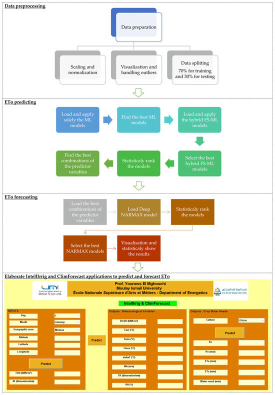
Figure 2.
A flowchart for the study methodology.
The methodology is structured into five main stages:
- Data Preprocessing: The process begins with loading the complete dataset, which is divided into training (70%) and testing (30%) subsets. Preprocessing steps include normalisation of the data and the application of an autonomous anomaly detection technique to identify and remove anomalous data points, thereby enhancing model reliability and accuracy.
- Machine Learning Model Evaluation: Thirteen machine learning (ML) models are trained and evaluated to determine their effectiveness in predicting and forecasting ETo. This comparative analysis is essential for identifying the most suitable ML model based on prediction performance metrics.
- Hybrid IFS-ML Model Implementation: A hybrid model combining integral feature selection (IFS) with the best-performing ML model is employed to identify the most informative predictor variables. This step involves an exhaustive search across all possible combinations of input features, systematically eliminating irrelevant or redundant combinations and retaining only those that yield the highest predictive accuracy.
- Deep NARMAX Model Integration: The optimal predictor combinations derived from the hybrid IFS-ML model are then fed into a Deep NARMAX model. This integration leverages the strengths of both ML-based feature selection and deep NARMAX’s nonlinear dynamic modelling capability to perform multi-step-ahead forecasting of ETo. Model parameters and forecasting formulas are iteratively refined and adapted during this stage.
- Application Development and Deployment: Finally, the entire predictive framework is encapsulated into a user-friendly application designed to facilitate efficient and accessible ETo prediction and forecasting. This step involves deploying the trained models into an interactive environment for real-time or batch predictions.
2.3.2. Solar Photovoltaic-Thermal Simulation Using ANSYS Fluent
Solar photovoltaic-thermal (PVT) systems refer to PV systems integrated with a cooling network. Typically, this cooling is achieved by circulating a designated fluid (water in this study). The water circulated within the PVT system can be used for irrigation, mainly through an underground irrigation system. The water delivered to the crops must maintain an optimal temperature and quantity. These parameters may vary depending on the design of the pumping system and prevailing climatic conditions.
The PVT system proposed for water irrigation was simulated using ANSYS Fluent 19.2. Initially, the simulation focused on the PV system alone, considering two different irradiance values (800 W/m2 and 1000 W/m2) to demonstrate their impact on the output power generated. Subsequently, two scenarios were tested for equipping the PV system with a cooling network—scaled PVT and coiled PVT—with both utilising water as the flowing fluid. ANSYS Fluent has been widely employed in previous research to investigate water flow within PV panels for two primary purposes: cooling the PV panel and generating water with various temperatures [54,55].
3. Results and Discussion
3.1. PVT Solutions
The proposed system involves circulating water through the PVT system before delivering it to the crops. Additionally, the electricity generated from the PVT can power the pump used in the irrigation process. This integrated approach represents a novel endeavour.
Based on ANSYS Fluent simulations, we analysed the temperature distribution of a specific PV module without a cooling-equipped network, considering two solar irradiance values: 800 W/m2 and 1000 W/m2 (see Figure 3). The results indicate that the temperature within the PV module ranged from 51.895 °C to 53.523 °C for insolation of 800 W/m2 and from 59.368 °C to 61.403 °C for insolation of 1000 W/m2. Notably, the PV panel was completely exposed to solar radiation in this simulation. These results show that high irradiance levels can significantly elevate the temperature of the PV panel, consequently reducing the efficiency of the PV system. Hence, we investigated the same PV panel under similar irradiances with two cooling options: scaled PVT and coiled PVT. Figure 4 demonstrates the temperature distribution for scaled PVT (a) at 800 W/m2 solar irradiance and (b) at 1000 W/m2 solar irradiance. As a result, the PV panel temperature could decrease by approximately 14 °C and 15 °C for 800 W/m2 and 1000 W/m2 solar irradiance, respectively. This significant reduction in temperature undoubtedly enhances the effectiveness of the PV system and increases the electricity produced for pumping and irrigation purposes.

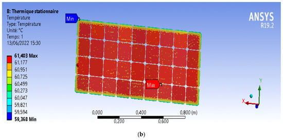
Figure 3.
PV module temperature distribution without cooling systems under solar irradiance of 800 W/m2 (a) and 1000 W/m2 (b).

Figure 4.
PV module temperature distribution for the scaled PVT system under solar irradiance of 800 W/m2 (a) and 1000 W/m2 (b).
With the scaled PVT solution, the PV panel temperature varied between 26.747 °C and 40.963 °C for 800 W/m2 solar flux and between 26.51 °C and 44.672 °C for 1000 W/m2 solar flux. This indicates an improvement in PV efficiency of approximately 7.32% and 10.02% for both irradiances, as summarised in Table 4.
Table 4.
Performance comparison of PV modules with and without cooling system.
Figure 5 illustrates the temperature distribution for coiled PVT (a) at 800 W/m2 solar irradiance and (b) at 1000 W/m2 solar irradiance. In this scenario, the temperature within the PV panel varied between 19.398 °C and 51.378 °C for 800 W/m2 irradiance and between 21.018 °C and 46.088 °C for 1000 W/m2 irradiance. There was a reduction in temperature of approximately 2 °C and 15 °C for 800 W/m2 and 1000 W/m2, respectively. This indicates an enhancement in the PV efficiency of approximately 2.94% and 9.72% for both solar fluxes, as summarised in Table 4.
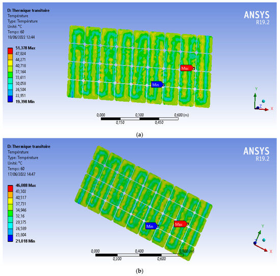
Figure 5.
PV module temperature distribution for the coiled PVT system under solar irradiance of 800 W/m2 (a) and 1000 W/m2 (b).
Based on the simulations and calculations, we observed a positive improvement rate, with a maximum value of approximately 10% for the scaled PVT module at 1000 W/m2. A positive improvement rate indicates that the performance of the scaled PVT solution was more effective than that of the coiled PVT solution. Consequently, we can infer that scaled PVT collectors play a significant role in reducing PV panel temperatures, thereby increasing electrical efficiency compared with conventional PV collectors. Additional results are summarised in Table 4.
3.2. Correlation Between Variables
This subsection investigates the intricate relationships between ETo and the various meteorological variables in Table 2. The primary objective is to uncover and analyse the underlying interdependence and correlations between ETo and these influencing factors. Understanding these connections is vital for developing accurate models, enhancing prediction and forecasting capabilities, and supporting informed decision making in the context of sustainable agriculture.
Figure 6 highlights the main factors influencing ETo. Solar irradiance was the most significant meteorological parameter affecting ETo (R2 = 0.89). Following this, Tmax and Tmoy exhibited notable importance (R2 = 0.70 and R2 = 0.67, respectively). Tmin demonstrated a moderate influence on ETo. Conversely, the correlation with precipitation, wind speed, and direction was weak, ranging between −0.23 and 0.13. Relative humidity showed negative and moderate correlations with ETo (R2 between −0.44 and −0.55), indicating an inverse relationship between ETo and RH.
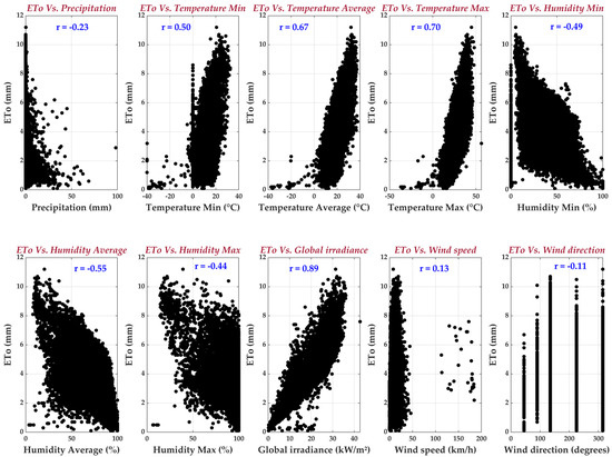
Figure 6.
ETo versus the studied variables.
3.3. Best ML Models for Predicting ETo
In this subsection, we conduct a comparative analysis of 13 different ML models for ETo prediction, emphasising their prediction accuracy and suitability for agricultural applications. The results of the comparison are depicted in Figure 7. Each studied ML model demonstrated unique strengths and weaknesses in ETo prediction. During the training stage, the decision tree (DT) emerged as the best-performing model, whereas during the testing stage, the tree bagger (TreeBag) model outperformed the others. The R2 values exceeded the level of confidence (R2 = 0.95) and approached one, indicating the highest level of accuracy prediction achieved by the best-performing models.
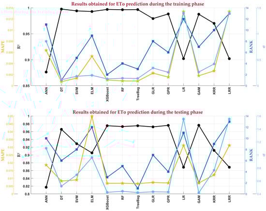
Figure 7.
A comparison of ML-based models for ETo predictions.
3.4. Best Hybrid IFS-ML Models for Predicting ETo
In this subsection, we employ hybrid IFS-ML models to identify the optimal combinations of meteorological variables for predicting ETo with the highest possible correlation and accuracy. The ML model previously selected as the top performer from the testing stage is utilised here. The performance analysis was initially based on the values of R2 (values superior to 0.95). Subsequently, all models are ranked based on the performance score φ, and the corresponding statistical indicators are summarised. In total, 1024 possible combinations were compared and assessed for predicting ETo.
The results obtained are presented in Figure 8 and Figure 9. A total of 301 best combinations of meteorological variables for predicting ETo were identified. Solar irradiance (H) emerged as the most crucial variable in all identified best combinations. This underscores the indispensability of H as a predictor in ETo modelling and prediction. The second most important variable was Tmax, present in 237 identified combinations. None of the combinations yielded ETo predictions based on just one or two input variables. Further insights can be gleaned from the same figures.
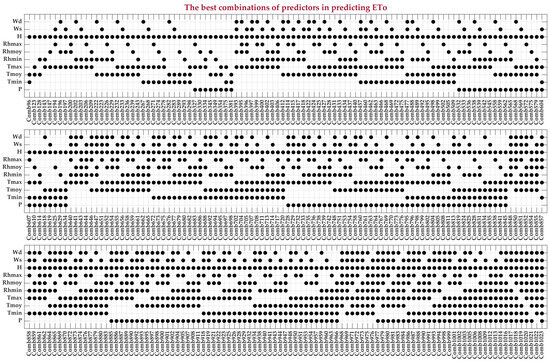
Figure 8.
The best combinations of inputs for ETo prediction.
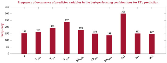
Figure 9.
Frequency of the studied input variables in best-performing combinations for ETo prediction.
To further evaluate the best-found combinations, Figure 10 presents a Taylor diagram for visualising their performance. The Taylor diagram is widely utilised for ranking models based on their standard deviation (σ), RMSE, and R2 values. A point closer to the left and downward corresponds to a model with better performance. As illustrated, the best-found combinations were plotted with the optimal values for indicators of dispersion and R2. This suggests that these top models have the potential to predict ETo with nearly perfect correlation and minimal error.
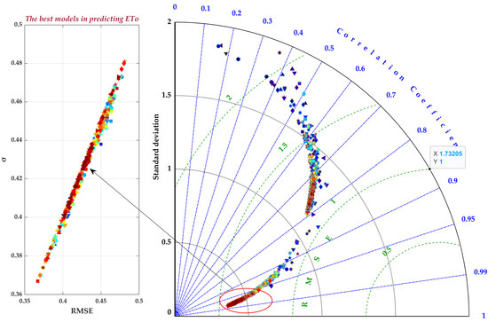
Figure 10.
Taylor diagram illustrating the performance of the best-performing combinations.
Moreover, based on the best combinations of predictors identified here and utilising the least squares method, 301 linear formulas have been elaborated and summarised in Appendix A, alongside the corresponding statistical analysis.
3.5. Best Models for Forecasting ETo
Accurate forecasting of future ETo is essential for enabling proactive climate adaptation strategies and safeguarding agricultural sustainability. In this subsection, the optimal predictor combinations identified through prior feature selection processes are integrated into the Deep NARMAX framework to model and forecast upcoming periods of ETo. By harnessing the powerful nonlinear modelling capabilities of the Deep NARMAX architecture, the objective is to generate robust and reliable forecasts that effectively capture the complex dynamics among meteorological variables.
To demonstrate the performance of the top-performing Deep NARMAX configurations, Figure 11 presents the multi-step-ahead time series forecast of daily ETo. This illustration includes the predicted ETo values, corresponding prediction errors, as well as key performance indicators, such as RMSE and R2 values. The most accurate model identified leveraged historical values of ETo at time steps t − 1 and t − 5, the minimum temperature at t − 5, and solar irradiance at t − 5. The statistical evaluation of this model indicates strong predictive performance, with error dispersion measures approaching zero and an R2 value nearing unity, suggesting a high level of model accuracy.
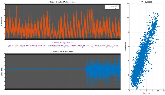
Figure 11.
The best NARMAX model for forecasting ETo.
Moreover, Appendix A provides a comprehensive set of elaborated forecasting formulas for the best-performing models and detailed statistical analyses. In total, 28 Deep NARMAX models were constructed and tested, utilising diverse combinations of historical time lags and meteorological predictors to forecast the next ETo period.
3.6. Application for Predicting and Forecasting ETo and Water Needs
Based on the best combination of meteorological variables discovered here and the best models developed for predicting and forecasting ETo, we created two applications: IntellIrrig and ClimForecast (see Figure 12). These applications cater to specific domains, with IntellIrrig focusing on agriculture, particularly intelligent irrigation, and ClimForecast targeting fields interested in atmospheric climate (meteorology). With IntellIrrig, users can determine the water requirement for a specific plant or crop at a given agricultural site by estimating the value of the reference evapotranspiration (ETo). On the other hand, ClimForecast enables users to predict and accurately forecast the most important meteorological parameters, such as solar radiation intensity, temperature, relative humidity, and wind speed.
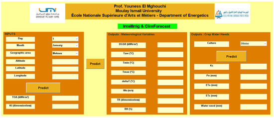
Figure 12.
IntellIrrig and ClimForecast applications developed for the prediction and forecasting of ETo, water requirements, and associated meteorological variables.
To accurately estimate crop water requirements, the reference evapotranspiration (ETo) was first calculated using the ClimForecast application, incorporating key meteorological variables such as global solar radiation, air temperature, humidity, and wind speed. Subsequently, the IntellIrrig application was used to compute ETo and crop water requirements based on the type of crop and its water needs under various climatic conditions.
In addition, this study investigated the influence of ambient temperature on photovoltaic (PV) systems, and it proposes using photovoltaic-thermal (PVT) systems as an optimal solution. PVT systems offer the dual benefit of reducing the PV module temperature—thereby improving energy efficiency—and capturing thermal energy through a heat exchange fluid. This recovered heat can be used to irrigate crops with water at a controlled temperature, which is particularly advantageous for certain plants during cold seasons or in colder climates.
This integrated approach does not replace observed meteorological data when available but serves as a sensitivity analysis to explore how PVT-induced thermal modifications may affect local microclimates and, in turn, influence irrigation requirements. Finally, the irrigation demand is calculated by adjusting ETo with crop-specific coefficients and accounting for effective precipitation, aiming to provide more realistic and adaptive water management under combined energy–agriculture scenarios.
4. Conclusions
In this study, a comprehensive predictive framework combining hybrid machine learning (ML) and deep learning (DL) models was developed and applied to model, predict, and forecast reference evapotranspiration (ETo) as a basis for estimating crop water requirements under varying climatic conditions. The methodology included data preprocessing with anomaly detection, model comparison, integral feature selection, and Deep NARMAX forecasting model integration. The results demonstrated high prediction accuracy, particularly with the hybrid IFS-ML and Deep NARMAX models, outperforming traditional AI-based models in multi-step-ahead forecasting scenarios.
Based on the experimental results and performance analysis, the following conclusions are drawn:
- High Accuracy in ETo Prediction: Among the 13 evaluated models, the hybrid approach integrating feature selection with Deep NARMAX achieved superior forecasting performance, reduced prediction error, and improved reliability in capturing nonlinear temporal dependencies in ETo dynamics.
- Effective Feature Selection for Climate-Driven Forecasting: The integral feature selection method successfully identified the most relevant meteorological variables influencing ETo, enhancing model interpretability and reducing computational complexity without compromising accuracy.
- Potential for Intelligent Irrigation Integration: The proposed predictive model is a foundational component for intelligent irrigation systems. When coupled with real-time sensor data and photovoltaic-thermal (PVT) systems, this model can facilitate dynamic irrigation scheduling, improving water use efficiency in agriculture.
- Implications for Sustainable Agriculture: By incorporating PVT systems into the forecasting and irrigation pipeline, there is potential to utilise renewable energy for both electricity and thermal applications in agriculture. This integration supports sustainable practices by reducing fossil fuel dependence and improving overall system energy efficiency.
- Scalability across Climatic Zones: The framework’s modularity and data-driven nature make it adaptable to diverse agro-climatic regions, allowing for its application in water-scarce and humid environments with appropriate local calibration.
This study demonstrates the viability and accuracy of ML and DL approaches for ETo forecasting and supports their future use in automated, sustainable irrigation management systems.
Author Contributions
Conceptualisation, Y.E.M. and M.T.U.; methodology, Y.E.M.; software, Y.E.M.; formal analysis, Y.E.M. and M.T.U.; investigation, Y.E.M. and M.T.U.; resources, M.T.U.; writing—original draft preparation, Y.E.M. and M.T.U.; writing—review and editing, Y.E.M. and M.T.U.; visualisation, Y.E.M.; supervision, Y.E.M. All authors have read and agreed to the published version of the manuscript.
Funding
This research received no external funding.
Institutional Review Board Statement
Not applicable.
Data Availability Statement
(1) The dataset, models, or codes supporting this study’s fundings are available from the corresponding author upon a reasonable request. (2) All data, models, and code generated or used during this study appear in the submitted article.
Conflicts of Interest
The authors declare no conflicts of interest.
Appendix A
Table A1.
Best models for predicting ETo.
Table A1.
Best models for predicting ETo.
| ModelID | a0 | a1 | a2 | a3 | a4 | a5 | a6 | a7 | a8 | a9 | a10 | MBE | RMSE | MAPE | Sd | R | Rank |
|---|---|---|---|---|---|---|---|---|---|---|---|---|---|---|---|---|---|
| Model1 | −1.446 | −0.077 | 0.167 | 0.171 | 0 | 0 | 0 | 0 | 0 | 0 | 0 | −0.049 | 0.499 | 0.003 | 0.497 | 0.959 | 299 |
| Model2 | −1.682 | −0.009 | 0.100 | 0.171 | 0 | 0 | 0 | 0 | 0 | 0 | 0 | −0.035 | 0.492 | 0.002 | 0.490 | 0.960 | 292 |
| Model3 | 0.132 | 0.080 | −0.019 | 0.167 | 0 | 0 | 0 | 0 | 0 | 0 | 0 | −0.012 | 0.418 | 0.002 | 0.418 | 0.971 | 233 |
| Model4 | −0.689 | 0.078 | −0.012 | 0.167 | 0 | 0 | 0 | 0 | 0 | 0 | 0 | −0.017 | 0.439 | 0.002 | 0.439 | 0.968 | 265 |
| Model5 | 0.575 | 0.068 | −0.021 | 0.166 | 0 | 0 | 0 | 0 | 0 | 0 | 0 | −0.009 | 0.380 | 0.002 | 0.380 | 0.976 | 104 |
| Model6 | 0.741 | 0.076 | −0.022 | 0.171 | 0.004 | 0 | 0 | 0 | 0 | 0 | 0 | −0.013 | 0.409 | 0.002 | 0.408 | 0.972 | 208 |
| Model7 | 0.750 | 0.069 | −0.022 | 0.165 | −0.001 | 0 | 0 | 0 | 0 | 0 | 0 | −0.015 | 0.379 | 0.002 | 0.378 | 0.976 | 115 |
| Model8 | 0.532 | 0.068 | −0.021 | 0.165 | 0.005 | 0 | 0 | 0 | 0 | 0 | 0 | −0.013 | 0.378 | 0.002 | 0.378 | 0.976 | 83 |
| Model9 | 0.730 | 0.068 | −0.019 | −0.004 | 0.167 | 0 | 0 | 0 | 0 | 0 | 0 | −0.007 | 0.379 | 0.002 | 0.379 | 0.976 | 100 |
| Model10 | −0.541 | 0.078 | −0.012 | 0.167 | −0.001 | 0 | 0 | 0 | 0 | 0 | 0 | −0.021 | 0.436 | 0.002 | 0.435 | 0.969 | 271 |
| Model11 | −0.719 | 0.078 | −0.012 | 0.166 | 0.006 | 0 | 0 | 0 | 0 | 0 | 0 | −0.021 | 0.436 | 0.002 | 0.435 | 0.969 | 270 |
| Model12 | 0.884 | 0.071 | −0.007 | −0.018 | 0.169 | 0 | 0 | 0 | 0 | 0 | 0 | −0.004 | 0.394 | 0.002 | 0.394 | 0.974 | 157 |
| Model13 | 0.628 | 0.069 | 0.003 | −0.024 | 0.166 | 0 | 0 | 0 | 0 | 0 | 0 | −0.010 | 0.379 | 0.002 | 0.378 | 0.976 | 103 |
| Model14 | 0.215 | 0.080 | −0.019 | 0.167 | 0 | 0 | 0 | 0 | 0 | 0 | 0 | −0.014 | 0.417 | 0.002 | 0.417 | 0.971 | 249 |
| Model15 | 0.118 | 0.080 | −0.019 | 0.166 | 0.004 | 0 | 0 | 0 | 0 | 0 | 0 | −0.015 | 0.417 | 0.002 | 0.417 | 0.971 | 248 |
| Model16 | 1.377 | 0.072 | −0.014 | −0.015 | 0.169 | 0 | 0 | 0 | 0 | 0 | 0 | −0.002 | 0.400 | 0.002 | 0.400 | 0.973 | 173 |
| Model17 | 1.223 | 0.070 | −0.005 | −0.021 | 0.167 | 0 | 0 | 0 | 0 | 0 | 0 | −0.007 | 0.386 | 0.002 | 0.386 | 0.975 | 132 |
| Model18 | −1.434 | −0.004 | 0.093 | 0.169 | −0.001 | 0 | 0 | 0 | 0 | 0 | 0 | −0.033 | 0.494 | 0.002 | 0.493 | 0.960 | 293 |
| Model19 | −1.742 | −0.014 | 0.104 | 0.170 | 0.005 | 0 | 0 | 0 | 0 | 0 | 0 | −0.039 | 0.490 | 0.002 | 0.489 | 0.960 | 289 |
| Model20 | 0.771 | −0.008 | 0.083 | −0.022 | 0.172 | 0 | 0 | 0 | 0 | 0 | 0 | −0.009 | 0.408 | 0.002 | 0.408 | 0.972 | 200 |
| Model21 | 0.797 | 0.028 | 0.043 | −0.023 | 0.166 | 0 | 0 | 0 | 0 | 0 | 0 | −0.009 | 0.375 | 0.002 | 0.375 | 0.977 | 43 |
| Model22 | −0.176 | 0.056 | 0.026 | −0.016 | 0.166 | 0 | 0 | 0 | 0 | 0 | 0 | −0.013 | 0.418 | 0.002 | 0.417 | 0.971 | 238 |
| Model23 | −1.639 | −0.017 | 0.105 | 0.169 | −0.001 | 0 | 0 | 0 | 0 | 0 | 0 | −0.039 | 0.486 | 0.002 | 0.484 | 0.961 | 284 |
| Model24 | −1.794 | −0.017 | 0.105 | 0.169 | 0.006 | 0 | 0 | 0 | 0 | 0 | 0 | −0.040 | 0.486 | 0.002 | 0.484 | 0.961 | 282 |
| Model25 | 0.702 | −0.011 | 0.084 | −0.022 | 0.171 | 0 | 0 | 0 | 0 | 0 | 0 | −0.010 | 0.404 | 0.002 | 0.404 | 0.973 | 191 |
| Model26 | 0.699 | 0.008 | 0.062 | −0.022 | 0.166 | 0 | 0 | 0 | 0 | 0 | 0 | −0.008 | 0.378 | 0.002 | 0.378 | 0.976 | 92 |
| Model27 | −0.299 | 0.020 | 0.059 | −0.015 | 0.167 | 0 | 0 | 0 | 0 | 0 | 0 | −0.011 | 0.429 | 0.002 | 0.429 | 0.970 | 251 |
| Model28 | −1.418 | −0.077 | 0.167 | 0.171 | 0 | 0 | 0 | 0 | 0 | 0 | 0 | −0.050 | 0.499 | 0.003 | 0.497 | 0.959 | 295 |
| Model29 | −1.476 | −0.078 | 0.168 | 0.171 | 0.003 | 0 | 0 | 0 | 0 | 0 | 0 | −0.051 | 0.499 | 0.003 | 0.497 | 0.959 | 296 |
| Model30 | 0.998 | −0.029 | 0.099 | −0.024 | 0.166 | 0 | 0 | 0 | 0 | 0 | 0 | −0.013 | 0.382 | 0.002 | 0.382 | 0.976 | 136 |
| Model31 | −0.021 | −0.014 | 0.094 | −0.017 | 0.166 | 0 | 0 | 0 | 0 | 0 | 0 | −0.014 | 0.417 | 0.002 | 0.417 | 0.971 | 243 |
| Model32 | −1.698 | −0.040 | 0.057 | 0.073 | 0.169 | 0 | 0 | 0 | 0 | 0 | 0 | −0.038 | 0.479 | 0.002 | 0.477 | 0.962 | 279 |
| Model33 | 0.769 | 0.008 | 0.077 | −0.022 | 0.172 | 0 | 0 | 0 | 0 | 0 | 0 | −0.010 | 0.409 | 0.002 | 0.409 | 0.972 | 205 |
| Model34 | 0.550 | 0.011 | 0.069 | −0.021 | 0.167 | 0 | 0 | 0 | 0 | 0 | 0 | −0.009 | 0.377 | 0.002 | 0.377 | 0.976 | 77 |
| Model35 | −0.716 | 0.011 | 0.078 | −0.012 | 0.168 | 0 | 0 | 0 | 0 | 0 | 0 | −0.017 | 0.437 | 0.002 | 0.436 | 0.969 | 266 |
| Model36 | 1.366 | 0.004 | 0.068 | −0.026 | 0.168 | 0 | 0 | 0 | 0 | 0 | 0 | −0.010 | 0.393 | 0.002 | 0.393 | 0.974 | 175 |
| Model37 | 0.122 | 0.006 | 0.080 | −0.019 | 0.168 | 0 | 0 | 0 | 0 | 0 | 0 | −0.012 | 0.417 | 0.002 | 0.417 | 0.971 | 229 |
| Model38 | −1.717 | 0.007 | −0.011 | 0.102 | 0.171 | 0 | 0 | 0 | 0 | 0 | 0 | −0.035 | 0.491 | 0.002 | 0.490 | 0.960 | 290 |
| Model39 | −1.773 | 0.008 | −0.016 | 0.105 | 0.171 | 0 | 0 | 0 | 0 | 0 | 0 | −0.036 | 0.487 | 0.002 | 0.485 | 0.961 | 283 |
| Model40 | −1.456 | 0.002 | −0.077 | 0.167 | 0.172 | 0 | 0 | 0 | 0 | 0 | 0 | −0.049 | 0.499 | 0.003 | 0.497 | 0.959 | 298 |
| Model41 | 0.730 | 0.068 | −0.022 | 0.165 | 0.003 | −0.001 | 0 | 0 | 0 | 0 | 0 | −0.016 | 0.378 | 0.002 | 0.378 | 0.976 | 118 |
| Model42 | 0.590 | 0.071 | −0.020 | −0.001 | 0.166 | −0.001 | 0 | 0 | 0 | 0 | 0 | −0.018 | 0.377 | 0.002 | 0.377 | 0.976 | 109 |
| Model43 | 0.665 | 0.068 | −0.019 | −0.003 | 0.166 | 0.005 | 0 | 0 | 0 | 0 | 0 | −0.011 | 0.378 | 0.002 | 0.378 | 0.976 | 80 |
| Model44 | −0.705 | 0.079 | −0.012 | 0.166 | 0.006 | 0 | 0 | 0 | 0 | 0 | 0 | −0.025 | 0.434 | 0.002 | 0.434 | 0.969 | 272 |
| Model45 | 0.579 | 0.076 | −0.007 | −0.015 | 0.169 | −0.001 | 0 | 0 | 0 | 0 | 0 | −0.015 | 0.391 | 0.002 | 0.391 | 0.975 | 177 |
| Model46 | 0.792 | 0.071 | −0.007 | −0.017 | 0.169 | 0.005 | 0 | 0 | 0 | 0 | 0 | −0.008 | 0.392 | 0.002 | 0.392 | 0.975 | 148 |
| Model47 | 0.306 | 0.075 | 0.002 | −0.021 | 0.168 | −0.001 | 0 | 0 | 0 | 0 | 0 | −0.022 | 0.377 | 0.002 | 0.376 | 0.976 | 125 |
| Model48 | 0.579 | 0.069 | 0.003 | −0.024 | 0.166 | 0.005 | 0 | 0 | 0 | 0 | 0 | −0.013 | 0.377 | 0.002 | 0.377 | 0.976 | 88 |
| Model49 | 0.552 | 0.070 | 0.003 | −0.024 | 0 | 0.167 | 0 | 0 | 0 | 0 | 0 | −0.012 | 0.378 | 0.002 | 0.378 | 0.976 | 98 |
| Model50 | 0.152 | 0.080 | −0.019 | 0.166 | 0.004 | 0 | 0 | 0 | 0 | 0 | 0 | −0.016 | 0.417 | 0.002 | 0.416 | 0.971 | 254 |
| Model51 | 1.160 | 0.075 | −0.015 | −0.012 | 0.170 | 0 | 0 | 0 | 0 | 0 | 0 | −0.010 | 0.398 | 0.002 | 0.398 | 0.974 | 178 |
| Model52 | 1.313 | 0.072 | −0.015 | −0.014 | 0.169 | 0.003 | 0 | 0 | 0 | 0 | 0 | −0.005 | 0.399 | 0.002 | 0.399 | 0.974 | 170 |
| Model53 | 0.838 | 0.075 | −0.007 | −0.016 | 0.169 | 0 | 0 | 0 | 0 | 0 | 0 | −0.018 | 0.385 | 0.002 | 0.385 | 0.975 | 167 |
| Model54 | 1.198 | 0.069 | −0.005 | −0.021 | 0.166 | 0.003 | 0 | 0 | 0 | 0 | 0 | −0.009 | 0.386 | 0.002 | 0.386 | 0.975 | 134 |
| Model55 | −1.571 | −0.012 | 0.101 | 0.169 | 0.004 | 0 | 0 | 0 | 0 | 0 | 0 | −0.036 | 0.492 | 0.002 | 0.491 | 0.960 | 291 |
| Model56 | 0.253 | −0.014 | 0.095 | −0.018 | 0.172 | −0.001 | 0 | 0 | 0 | 0 | 0 | −0.022 | 0.406 | 0.002 | 0.406 | 0.973 | 257 |
| Model57 | 0.682 | −0.012 | 0.086 | −0.022 | 0.171 | 0.004 | 0 | 0 | 0 | 0 | 0 | −0.013 | 0.407 | 0.002 | 0.407 | 0.973 | 207 |
| Model58 | 0.551 | 0.019 | 0.057 | −0.020 | 0.165 | −0.001 | 0 | 0 | 0 | 0 | 0 | −0.020 | 0.373 | 0.002 | 0.373 | 0.977 | 47 |
| Model59 | 0.732 | 0.025 | 0.046 | −0.022 | 0.165 | 0.004 | 0 | 0 | 0 | 0 | 0 | −0.012 | 0.374 | 0.002 | 0.374 | 0.977 | 32 |
| Model60 | 0.671 | 0.027 | 0.045 | −0.023 | 0.001 | 0.166 | 0 | 0 | 0 | 0 | 0 | −0.010 | 0.374 | 0.002 | 0.374 | 0.977 | 34 |
| Model61 | −0.097 | 0.053 | 0.029 | −0.016 | 0.166 | −0.001 | 0 | 0 | 0 | 0 | 0 | −0.016 | 0.416 | 0.002 | 0.416 | 0.971 | 253 |
| Model62 | −0.238 | 0.051 | 0.030 | −0.016 | 0.166 | 0.005 | 0 | 0 | 0 | 0 | 0 | −0.016 | 0.416 | 0.002 | 0.416 | 0.971 | 247 |
| Model63 | 1.014 | 0.031 | 0.042 | −0.010 | −0.016 | 0.169 | 0 | 0 | 0 | 0 | 0 | −0.003 | 0.390 | 0.002 | 0.390 | 0.975 | 140 |
| Model64 | 0.797 | 0.028 | 0.043 | 0 | −0.023 | 0.166 | 0 | 0 | 0 | 0 | 0 | −0.009 | 0.375 | 0.002 | 0.375 | 0.977 | 45 |
| Model65 | −1.736 | −0.018 | 0.106 | 0.169 | 0.005 | 0 | 0 | 0 | 0 | 0 | 0 | −0.041 | 0.485 | 0.002 | 0.483 | 0.961 | 281 |
| Model66 | 0.623 | −0.013 | 0.086 | −0.022 | 0.170 | 0.005 | 0 | 0 | 0 | 0 | 0 | −0.014 | 0.403 | 0.002 | 0.402 | 0.973 | 199 |
| Model67 | 0.681 | 0.004 | 0.067 | −0.021 | 0.166 | −0.001 | 0 | 0 | 0 | 0 | 0 | −0.016 | 0.377 | 0.002 | 0.377 | 0.976 | 101 |
| Model68 | 0.645 | 0.006 | 0.063 | −0.022 | 0.166 | 0.005 | 0 | 0 | 0 | 0 | 0 | −0.011 | 0.377 | 0.002 | 0.377 | 0.976 | 78 |
| Model69 | 0.701 | 0.007 | 0.063 | −0.021 | −0.001 | 0.167 | 0 | 0 | 0 | 0 | 0 | −0.008 | 0.378 | 0.002 | 0.378 | 0.976 | 87 |
| Model70 | −0.236 | 0.018 | 0.062 | −0.015 | 0.167 | −0.001 | 0 | 0 | 0 | 0 | 0 | −0.016 | 0.427 | 0.002 | 0.427 | 0.970 | 264 |
| Model71 | −0.367 | 0.018 | 0.061 | −0.015 | 0.166 | 0.006 | 0 | 0 | 0 | 0 | 0 | −0.016 | 0.427 | 0.002 | 0.426 | 0.970 | 261 |
| Model72 | 0.979 | 0.007 | 0.064 | −0.008 | −0.018 | 0.169 | 0 | 0 | 0 | 0 | 0 | −0.002 | 0.394 | 0.002 | 0.394 | 0.974 | 155 |
| Model73 | 0.630 | 0.004 | 0.066 | 0.002 | −0.023 | 0.166 | 0 | 0 | 0 | 0 | 0 | −0.010 | 0.378 | 0.002 | 0.378 | 0.976 | 94 |
| Model74 | −1.473 | −0.078 | 0.167 | 0.171 | 0.003 | 0 | 0 | 0 | 0 | 0 | 0 | −0.051 | 0.500 | 0.003 | 0.497 | 0.959 | 300 |
| Model75 | 0.046 | −0.015 | 0.096 | −0.017 | 0.166 | 0 | 0 | 0 | 0 | 0 | 0 | −0.018 | 0.416 | 0.002 | 0.416 | 0.971 | 255 |
| Model76 | −0.048 | −0.015 | 0.095 | −0.017 | 0.166 | 0.004 | 0 | 0 | 0 | 0 | 0 | −0.018 | 0.416 | 0.002 | 0.416 | 0.971 | 244 |
| Model77 | 1.181 | −0.022 | 0.095 | −0.012 | −0.015 | 0.169 | 0 | 0 | 0 | 0 | 0 | −0.006 | 0.396 | 0.002 | 0.396 | 0.974 | 161 |
| Model78 | 0.998 | −0.024 | 0.095 | −0.002 | −0.022 | 0.166 | 0 | 0 | 0 | 0 | 0 | −0.012 | 0.381 | 0.002 | 0.381 | 0.976 | 119 |
| Model79 | −1.657 | −0.040 | 0.054 | 0.077 | 0.169 | 0 | 0 | 0 | 0 | 0 | 0 | −0.043 | 0.477 | 0.002 | 0.475 | 0.962 | 274 |
| Model80 | −1.759 | −0.040 | 0.053 | 0.077 | 0.168 | 0.005 | 0 | 0 | 0 | 0 | 0 | −0.042 | 0.478 | 0.002 | 0.476 | 0.962 | 275 |
| Model81 | 0.546 | −0.029 | 0.040 | 0.065 | −0.021 | 0.170 | 0 | 0 | 0 | 0 | 0 | −0.014 | 0.400 | 0.002 | 0.400 | 0.973 | 196 |
| Model82 | 0.725 | −0.014 | 0.050 | 0.035 | −0.022 | 0.166 | 0 | 0 | 0 | 0 | 0 | −0.011 | 0.373 | 0.002 | 0.373 | 0.977 | 19 |
| Model83 | −0.221 | −0.008 | 0.067 | 0.023 | −0.016 | 0.166 | 0 | 0 | 0 | 0 | 0 | −0.014 | 0.417 | 0.002 | 0.417 | 0.971 | 240 |
| Model84 | 0.783 | 0.010 | 0.069 | −0.022 | 0.166 | −0.001 | 0 | 0 | 0 | 0 | 0 | −0.015 | 0.377 | 0.002 | 0.377 | 0.976 | 105 |
| Model85 | 0.492 | 0.009 | 0.069 | −0.021 | 0.166 | 0.005 | 0 | 0 | 0 | 0 | 0 | −0.013 | 0.376 | 0.002 | 0.376 | 0.977 | 53 |
| Model86 | 0.694 | 0.010 | 0.069 | −0.019 | −0.003 | 0.168 | 0 | 0 | 0 | 0 | 0 | −0.008 | 0.377 | 0.002 | 0.377 | 0.976 | 71 |
| Model87 | −0.547 | 0.011 | 0.078 | −0.012 | 0.167 | −0.001 | 0 | 0 | 0 | 0 | 0 | −0.021 | 0.434 | 0.002 | 0.433 | 0.969 | 269 |
| Model88 | −0.741 | 0.010 | 0.078 | −0.012 | 0.167 | 0.006 | 0 | 0 | 0 | 0 | 0 | −0.021 | 0.434 | 0.002 | 0.433 | 0.969 | 268 |
| Model89 | 0.862 | 0.010 | 0.071 | −0.007 | −0.018 | 0.170 | 0 | 0 | 0 | 0 | 0 | −0.004 | 0.392 | 0.002 | 0.392 | 0.974 | 152 |
| Model90 | 0.599 | 0.010 | 0.069 | 0.003 | −0.024 | 0.167 | 0 | 0 | 0 | 0 | 0 | −0.011 | 0.377 | 0.002 | 0.376 | 0.977 | 68 |
| Model91 | 0.148 | 0.007 | 0.081 | −0.019 | 0.168 | 0 | 0 | 0 | 0 | 0 | 0 | −0.016 | 0.416 | 0.002 | 0.416 | 0.971 | 250 |
| Model92 | 0.110 | 0.006 | 0.080 | −0.019 | 0.167 | 0.004 | 0 | 0 | 0 | 0 | 0 | −0.015 | 0.416 | 0.002 | 0.416 | 0.971 | 236 |
| Model93 | 1.366 | 0.006 | 0.072 | −0.015 | −0.015 | 0.170 | 0 | 0 | 0 | 0 | 0 | −0.003 | 0.400 | 0.002 | 0.400 | 0.973 | 171 |
| Model94 | 1.201 | 0.006 | 0.070 | −0.005 | −0.021 | 0.167 | 0 | 0 | 0 | 0 | 0 | −0.008 | 0.385 | 0.002 | 0.385 | 0.975 | 123 |
| Model95 | −1.639 | 0.006 | −0.013 | 0.105 | 0.171 | 0 | 0 | 0 | 0 | 0 | 0 | −0.038 | 0.490 | 0.002 | 0.489 | 0.960 | 287 |
| Model96 | −1.771 | 0.006 | −0.015 | 0.106 | 0.170 | 0.005 | 0 | 0 | 0 | 0 | 0 | −0.039 | 0.490 | 0.002 | 0.489 | 0.960 | 285 |
| Model97 | 0.722 | 0.008 | −0.010 | 0.085 | −0.022 | 0.172 | 0 | 0 | 0 | 0 | 0 | −0.010 | 0.407 | 0.002 | 0.407 | 0.972 | 201 |
| Model98 | 0.759 | 0.009 | 0.026 | 0.045 | −0.023 | 0.167 | 0 | 0 | 0 | 0 | 0 | −0.009 | 0.374 | 0.002 | 0.374 | 0.977 | 24 |
| Model99 | −0.213 | 0.008 | 0.054 | 0.028 | −0.016 | 0.167 | 0 | 0 | 0 | 0 | 0 | −0.013 | 0.416 | 0.002 | 0.416 | 0.971 | 227 |
| Model100 | −1.830 | 0.007 | −0.018 | 0.106 | 0.170 | 0.006 | 0 | 0 | 0 | 0 | 0 | −0.040 | 0.485 | 0.002 | 0.483 | 0.961 | 280 |
| Model101 | 0.660 | 0.010 | −0.013 | 0.086 | −0.022 | 0.172 | 0 | 0 | 0 | 0 | 0 | −0.011 | 0.403 | 0.002 | 0.403 | 0.973 | 193 |
| Model102 | 0.674 | 0.010 | 0.007 | 0.063 | −0.022 | 0.167 | 0 | 0 | 0 | 0 | 0 | −0.008 | 0.377 | 0.002 | 0.377 | 0.976 | 62 |
| Model103 | −0.342 | 0.009 | 0.019 | 0.060 | −0.015 | 0.168 | 0 | 0 | 0 | 0 | 0 | −0.012 | 0.427 | 0.002 | 0.427 | 0.970 | 252 |
| Model104 | −1.424 | 0.002 | −0.077 | 0.167 | 0.172 | 0 | 0 | 0 | 0 | 0 | 0 | −0.050 | 0.500 | 0.003 | 0.497 | 0.959 | 301 |
| Model105 | −1.482 | 0.001 | −0.078 | 0.168 | 0.171 | 0.003 | 0 | 0 | 0 | 0 | 0 | −0.052 | 0.499 | 0.003 | 0.497 | 0.959 | 297 |
| Model106 | 0.993 | 0.006 | −0.029 | 0.099 | −0.024 | 0.167 | 0 | 0 | 0 | 0 | 0 | −0.014 | 0.381 | 0.002 | 0.381 | 0.976 | 137 |
| Model107 | −0.040 | 0.007 | −0.015 | 0.095 | −0.017 | 0.167 | 0 | 0 | 0 | 0 | 0 | −0.015 | 0.416 | 0.002 | 0.416 | 0.971 | 226 |
| Model108 | −1.737 | 0.007 | −0.040 | 0.056 | 0.075 | 0.170 | 0 | 0 | 0 | 0 | 0 | −0.039 | 0.478 | 0.002 | 0.477 | 0.962 | 276 |
| Model109 | 0.196 | 0.078 | −0.007 | −0.012 | 0.169 | 0.005 | 0 | 0 | 0 | 0 | 0 | −0.021 | 0.392 | 0.002 | 0.392 | 0.975 | 190 |
| Model110 | 0.642 | 0.071 | 0.003 | −0.023 | 0.166 | 0.003 | −0.001 | 0 | 0 | 0 | 0 | −0.019 | 0.377 | 0.002 | 0.376 | 0.976 | 108 |
| Model111 | 0.534 | 0.072 | 0.003 | −0.025 | 0.002 | 0.166 | −0.001 | 0 | 0 | 0 | 0 | −0.020 | 0.377 | 0.002 | 0.376 | 0.976 | 113 |
| Model112 | 0.579 | 0.069 | 0.003 | −0.023 | −0.001 | 0.166 | 0.005 | 0 | 0 | 0 | 0 | −0.014 | 0.377 | 0.002 | 0.377 | 0.976 | 82 |
| Model113 | 0.379 | 0.080 | −0.015 | −0.006 | 0.170 | 0.005 | 0 | 0 | 0 | 0 | 0 | −0.020 | 0.402 | 0.002 | 0.402 | 0.973 | 215 |
| Model114 | 0.777 | 0.075 | −0.007 | −0.016 | 0.169 | 0.003 | 0 | 0 | 0 | 0 | 0 | −0.019 | 0.385 | 0.002 | 0.385 | 0.975 | 168 |
| Model115 | 0.666 | −0.002 | 0.077 | −0.021 | 0.176 | 0.003 | 0 | 0 | 0 | 0 | 0 | −0.020 | 0.412 | 0.002 | 0.412 | 0.972 | 259 |
| Model116 | 0.525 | 0.017 | 0.058 | −0.020 | 0.166 | 0.003 | −0.001 | 0 | 0 | 0 | 0 | −0.020 | 0.373 | 0.002 | 0.373 | 0.977 | 48 |
| Model117 | 0.167 | 0.022 | 0.056 | −0.022 | 0.005 | 0.166 | −0.001 | 0 | 0 | 0 | 0 | −0.024 | 0.377 | 0.002 | 0.376 | 0.977 | 111 |
| Model118 | 0.677 | 0.024 | 0.047 | −0.022 | 0 | 0.165 | 0.004 | 0 | 0 | 0 | 0 | −0.013 | 0.374 | 0.002 | 0.374 | 0.977 | 27 |
| Model119 | −0.128 | 0.052 | 0.029 | −0.017 | 0.165 | 0.004 | 0 | 0 | 0 | 0 | 0 | −0.017 | 0.416 | 0.002 | 0.415 | 0.971 | 237 |
| Model120 | 1.007 | 0.025 | 0.050 | −0.009 | −0.016 | 0.168 | −0.001 | 0 | 0 | 0 | 0 | −0.010 | 0.389 | 0.002 | 0.389 | 0.975 | 142 |
| Model121 | 0.866 | 0.027 | 0.047 | −0.010 | −0.016 | 0.168 | 0.005 | 0 | 0 | 0 | 0 | −0.008 | 0.388 | 0.002 | 0.388 | 0.975 | 126 |
| Model122 | 1.030 | 0.023 | 0.047 | 0.001 | −0.024 | 0.165 | −0.001 | 0 | 0 | 0 | 0 | −0.013 | 0.377 | 0.002 | 0.377 | 0.976 | 99 |
| Model123 | 0.667 | 0.023 | 0.048 | 0 | −0.022 | 0.166 | 0.004 | 0 | 0 | 0 | 0 | −0.013 | 0.374 | 0.002 | 0.374 | 0.977 | 28 |
| Model124 | 0.853 | 0.029 | 0.042 | 0 | −0.023 | 0 | 0.166 | 0 | 0 | 0 | 0 | −0.008 | 0.376 | 0.002 | 0.376 | 0.977 | 54 |
| Model125 | 0.427 | −0.015 | 0.091 | −0.020 | 0.170 | 0.004 | −0.001 | 0 | 0 | 0 | 0 | −0.022 | 0.401 | 0.002 | 0.401 | 0.973 | 235 |
| Model126 | 0.816 | 0.005 | 0.064 | −0.022 | 0.165 | 0.003 | −0.001 | 0 | 0 | 0 | 0 | −0.015 | 0.378 | 0.002 | 0.378 | 0.976 | 110 |
| Model127 | 0.312 | 0.003 | 0.071 | −0.020 | 0.002 | 0.166 | −0.001 | 0 | 0 | 0 | 0 | −0.020 | 0.378 | 0.002 | 0.378 | 0.976 | 120 |
| Model128 | 0.625 | 0.005 | 0.065 | −0.021 | −0.001 | 0.166 | 0.005 | 0 | 0 | 0 | 0 | −0.012 | 0.377 | 0.002 | 0.377 | 0.976 | 67 |
| Model129 | −0.220 | 0.019 | 0.059 | −0.016 | 0.166 | 0.005 | 0 | 0 | 0 | 0 | 0 | −0.016 | 0.426 | 0.002 | 0.425 | 0.970 | 262 |
| Model130 | 1.111 | 0.004 | 0.068 | −0.008 | −0.018 | 0.169 | −0.001 | 0 | 0 | 0 | 0 | −0.009 | 0.394 | 0.002 | 0.394 | 0.974 | 163 |
| Model131 | 0.365 | 0.001 | 0.074 | −0.007 | −0.014 | 0.169 | 0.005 | 0 | 0 | 0 | 0 | −0.015 | 0.391 | 0.002 | 0.390 | 0.975 | 165 |
| Model132 | 0.208 | −0.005 | 0.080 | 0.004 | −0.021 | 0.168 | −0.001 | 0 | 0 | 0 | 0 | −0.025 | 0.378 | 0.002 | 0.378 | 0.976 | 150 |
| Model133 | 0.543 | 0.002 | 0.068 | 0.002 | −0.023 | 0.166 | 0.005 | 0 | 0 | 0 | 0 | −0.014 | 0.377 | 0.002 | 0.376 | 0.976 | 76 |
| Model134 | 0.634 | 0.004 | 0.066 | 0.002 | −0.024 | 0 | 0.166 | 0 | 0 | 0 | 0 | −0.009 | 0.378 | 0.002 | 0.378 | 0.976 | 89 |
| Model135 | 0.700 | −0.039 | 0.112 | −0.021 | 0.167 | 0.003 | 0 | 0 | 0 | 0 | 0 | −0.026 | 0.381 | 0.002 | 0.380 | 0.976 | 179 |
| Model136 | −0.001 | −0.015 | 0.095 | −0.017 | 0.166 | 0.004 | 0 | 0 | 0 | 0 | 0 | −0.019 | 0.416 | 0.002 | 0.415 | 0.971 | 245 |
| Model137 | 0.193 | −0.036 | 0.118 | −0.011 | −0.008 | 0.170 | 0 | 0 | 0 | 0 | 0 | −0.025 | 0.399 | 0.002 | 0.398 | 0.974 | 214 |
| Model138 | 0.969 | −0.026 | 0.100 | −0.012 | −0.014 | 0.168 | 0.004 | 0 | 0 | 0 | 0 | −0.012 | 0.393 | 0.002 | 0.393 | 0.974 | 166 |
| Model139 | 0.795 | −0.034 | 0.109 | −0.002 | −0.020 | 0.166 | −0.001 | 0 | 0 | 0 | 0 | −0.022 | 0.380 | 0.002 | 0.379 | 0.976 | 159 |
| Model140 | 0.967 | −0.025 | 0.095 | −0.002 | −0.022 | 0.166 | 0.003 | 0 | 0 | 0 | 0 | −0.014 | 0.381 | 0.002 | 0.380 | 0.976 | 133 |
| Model141 | −1.187 | −0.040 | 0.060 | 0.062 | 0.165 | 0.001 | −0.001 | 0 | 0 | 0 | 0 | −0.033 | 0.494 | 0.002 | 0.493 | 0.961 | 286 |
| Model142 | 0.307 | −0.031 | 0.038 | 0.073 | −0.018 | 0.170 | −0.001 | 0 | 0 | 0 | 0 | −0.025 | 0.399 | 0.002 | 0.398 | 0.974 | 232 |
| Model143 | 0.604 | −0.029 | 0.037 | 0.067 | −0.021 | 0.170 | 0.004 | 0 | 0 | 0 | 0 | −0.016 | 0.400 | 0.002 | 0.400 | 0.973 | 202 |
| Model144 | 0.105 | −0.021 | 0.047 | 0.053 | −0.017 | 0.167 | −0.001 | 0 | 0 | 0 | 0 | −0.026 | 0.375 | 0.002 | 0.374 | 0.977 | 91 |
| Model145 | 0.515 | −0.015 | 0.047 | 0.041 | −0.021 | 0.165 | 0.004 | 0 | 0 | 0 | 0 | −0.016 | 0.372 | 0.002 | 0.371 | 0.977 | 10 |
| Model146 | 0.700 | −0.014 | 0.050 | 0.036 | −0.021 | 0 | 0.166 | 0 | 0 | 0 | 0 | −0.011 | 0.373 | 0.002 | 0.373 | 0.977 | 12 |
| Model147 | −0.027 | −0.006 | 0.066 | 0.021 | −0.017 | 0.165 | −0.001 | 0 | 0 | 0 | 0 | −0.016 | 0.416 | 0.002 | 0.416 | 0.971 | 228 |
| Model148 | −0.297 | −0.008 | 0.063 | 0.027 | −0.016 | 0.166 | 0.005 | 0 | 0 | 0 | 0 | −0.018 | 0.416 | 0.002 | 0.416 | 0.971 | 242 |
| Model149 | 0.441 | −0.017 | 0.048 | 0.046 | −0.008 | −0.013 | 0.169 | 0 | 0 | 0 | 0 | −0.013 | 0.387 | 0.002 | 0.387 | 0.975 | 143 |
| Model150 | 0.600 | −0.017 | 0.049 | 0.040 | 0.002 | −0.022 | 0.166 | 0 | 0 | 0 | 0 | −0.013 | 0.373 | 0.002 | 0.372 | 0.977 | 15 |
| Model151 | 0.496 | 0.007 | 0.080 | −0.020 | 0.172 | 0.003 | 0 | 0 | 0 | 0 | 0 | −0.021 | 0.407 | 0.002 | 0.406 | 0.973 | 256 |
| Model152 | 0.279 | 0.010 | 0.074 | −0.019 | 0.167 | 0.004 | 0 | 0 | 0 | 0 | 0 | −0.022 | 0.375 | 0.002 | 0.375 | 0.977 | 81 |
| Model153 | 0.633 | 0.009 | 0.069 | −0.020 | −0.003 | 0.167 | 0.004 | 0 | 0 | 0 | 0 | −0.012 | 0.376 | 0.002 | 0.376 | 0.977 | 50 |
| Model154 | −0.401 | 0.009 | 0.074 | −0.014 | 0.166 | 0.004 | −0.001 | 0 | 0 | 0 | 0 | −0.019 | 0.434 | 0.002 | 0.433 | 0.969 | 267 |
| Model155 | 0.435 | 0.011 | 0.077 | −0.007 | −0.014 | 0.170 | −0.001 | 0 | 0 | 0 | 0 | −0.017 | 0.390 | 0.002 | 0.389 | 0.975 | 181 |
| Model156 | 0.667 | 0.010 | 0.072 | −0.007 | −0.017 | 0.170 | 0.005 | 0 | 0 | 0 | 0 | −0.010 | 0.389 | 0.002 | 0.389 | 0.975 | 141 |
| Model157 | 0.819 | 0.009 | 0.069 | 0.003 | −0.025 | 0.166 | −0.001 | 0 | 0 | 0 | 0 | −0.016 | 0.377 | 0.002 | 0.377 | 0.976 | 112 |
| Model158 | 0.526 | 0.009 | 0.070 | 0.002 | −0.024 | 0.167 | 0.004 | 0 | 0 | 0 | 0 | −0.014 | 0.375 | 0.002 | 0.375 | 0.977 | 55 |
| Model159 | 0.487 | 0.010 | 0.070 | 0.003 | −0.024 | 0 | 0.167 | 0 | 0 | 0 | 0 | −0.013 | 0.376 | 0.002 | 0.376 | 0.977 | 65 |
| Model160 | 0.145 | 0.006 | 0.080 | −0.019 | 0.167 | 0.004 | 0 | 0 | 0 | 0 | 0 | −0.016 | 0.416 | 0.002 | 0.415 | 0.971 | 239 |
| Model161 | 1.417 | 0.005 | 0.071 | −0.015 | −0.015 | 0.169 | 0.003 | 0 | 0 | 0 | 0 | −0.003 | 0.400 | 0.002 | 0.400 | 0.973 | 174 |
| Model162 | 0.358 | 0.007 | 0.081 | −0.009 | −0.011 | 0.172 | 0 | 0 | 0 | 0 | 0 | −0.024 | 0.392 | 0.002 | 0.391 | 0.975 | 204 |
| Model163 | 1.102 | 0.005 | 0.071 | −0.006 | −0.020 | 0.167 | 0.003 | 0 | 0 | 0 | 0 | −0.012 | 0.384 | 0.002 | 0.384 | 0.975 | 130 |
| Model164 | −1.677 | 0.005 | −0.014 | 0.104 | 0.170 | 0.004 | 0 | 0 | 0 | 0 | 0 | −0.039 | 0.490 | 0.002 | 0.489 | 0.960 | 288 |
| Model165 | 0.674 | 0.008 | −0.016 | 0.092 | −0.021 | 0.172 | −0.001 | 0 | 0 | 0 | 0 | −0.016 | 0.406 | 0.002 | 0.406 | 0.973 | 213 |
| Model166 | 0.634 | 0.008 | −0.014 | 0.089 | −0.022 | 0.172 | 0.004 | 0 | 0 | 0 | 0 | −0.013 | 0.406 | 0.002 | 0.406 | 0.973 | 206 |
| Model167 | 0.374 | 0.010 | 0.014 | 0.063 | −0.019 | 0.168 | −0.001 | 0 | 0 | 0 | 0 | −0.021 | 0.373 | 0.002 | 0.372 | 0.977 | 49 |
| Model168 | 0.698 | 0.008 | 0.023 | 0.048 | −0.023 | 0.166 | 0.004 | 0 | 0 | 0 | 0 | −0.012 | 0.373 | 0.002 | 0.373 | 0.977 | 14 |
| Model169 | 0.528 | 0.009 | 0.025 | 0.049 | −0.023 | 0.002 | 0.167 | 0 | 0 | 0 | 0 | −0.013 | 0.373 | 0.002 | 0.373 | 0.977 | 11 |
| Model170 | −0.079 | 0.008 | 0.053 | 0.028 | −0.017 | 0.167 | −0.001 | 0 | 0 | 0 | 0 | −0.016 | 0.415 | 0.002 | 0.415 | 0.972 | 216 |
| Model171 | −0.243 | 0.007 | 0.051 | 0.030 | −0.016 | 0.166 | 0.005 | 0 | 0 | 0 | 0 | −0.016 | 0.415 | 0.002 | 0.415 | 0.972 | 220 |
| Model172 | 0.794 | 0.009 | 0.027 | 0.048 | −0.010 | −0.015 | 0.170 | 0 | 0 | 0 | 0 | −0.007 | 0.387 | 0.002 | 0.387 | 0.975 | 124 |
| Model173 | 0.561 | 0.009 | 0.022 | 0.052 | 0 | −0.021 | 0.167 | 0 | 0 | 0 | 0 | −0.012 | 0.373 | 0.002 | 0.372 | 0.977 | 16 |
| Model174 | 0.862 | 0.009 | −0.015 | 0.088 | −0.023 | 0.171 | −0.001 | 0 | 0 | 0 | 0 | −0.017 | 0.405 | 0.002 | 0.405 | 0.973 | 217 |
| Model175 | 0.517 | 0.009 | −0.014 | 0.088 | −0.021 | 0.171 | 0.005 | 0 | 0 | 0 | 0 | −0.016 | 0.401 | 0.002 | 0.400 | 0.973 | 203 |
| Model176 | 0.314 | 0.011 | 0 | 0.075 | −0.019 | 0.168 | −0.001 | 0 | 0 | 0 | 0 | −0.021 | 0.375 | 0.002 | 0.375 | 0.977 | 90 |
| Model177 | 0.573 | 0.009 | 0.005 | 0.065 | −0.022 | 0.166 | 0.004 | 0 | 0 | 0 | 0 | −0.013 | 0.375 | 0.002 | 0.375 | 0.977 | 44 |
| Model178 | 0.648 | 0.010 | 0.006 | 0.065 | −0.021 | −0.001 | 0.168 | 0 | 0 | 0 | 0 | −0.009 | 0.376 | 0.002 | 0.376 | 0.977 | 58 |
| Model179 | −0.248 | 0.009 | 0.018 | 0.062 | −0.015 | 0.168 | −0.001 | 0 | 0 | 0 | 0 | −0.016 | 0.425 | 0.002 | 0.425 | 0.970 | 263 |
| Model180 | −0.396 | 0.008 | 0.017 | 0.062 | −0.015 | 0.167 | 0.005 | 0 | 0 | 0 | 0 | −0.016 | 0.425 | 0.002 | 0.425 | 0.970 | 260 |
| Model181 | 0.916 | 0.010 | 0.006 | 0.066 | −0.008 | −0.017 | 0.170 | 0 | 0 | 0 | 0 | −0.003 | 0.392 | 0.002 | 0.392 | 0.974 | 149 |
| Model182 | 0.637 | 0.010 | 0.003 | 0.066 | 0.002 | −0.024 | 0.167 | 0 | 0 | 0 | 0 | −0.010 | 0.376 | 0.002 | 0.376 | 0.977 | 63 |
| Model183 | −1.488 | 0.001 | −0.078 | 0.168 | 0.171 | 0.003 | 0 | 0 | 0 | 0 | 0 | −0.052 | 0.499 | 0.003 | 0.497 | 0.959 | 294 |
| Model184 | 0.961 | 0.006 | −0.030 | 0.100 | −0.024 | 0.167 | 0.003 | 0 | 0 | 0 | 0 | −0.016 | 0.381 | 0.002 | 0.381 | 0.976 | 147 |
| Model185 | 0.018 | 0.007 | −0.016 | 0.097 | −0.017 | 0.167 | 0 | 0 | 0 | 0 | 0 | −0.018 | 0.415 | 0.002 | 0.415 | 0.972 | 241 |
| Model186 | −0.063 | 0.006 | −0.016 | 0.096 | −0.017 | 0.167 | 0.004 | 0 | 0 | 0 | 0 | −0.018 | 0.415 | 0.002 | 0.415 | 0.972 | 230 |
| Model187 | 1.015 | 0.007 | −0.025 | 0.099 | −0.012 | −0.014 | 0.170 | 0 | 0 | 0 | 0 | −0.009 | 0.393 | 0.002 | 0.393 | 0.974 | 162 |
| Model188 | 0.921 | 0.007 | −0.026 | 0.098 | −0.002 | −0.021 | 0.167 | 0 | 0 | 0 | 0 | −0.014 | 0.379 | 0.002 | 0.379 | 0.976 | 121 |
| Model189 | −1.614 | 0.007 | −0.041 | 0.055 | 0.076 | 0.169 | −0.001 | 0 | 0 | 0 | 0 | −0.041 | 0.478 | 0.002 | 0.476 | 0.962 | 277 |
| Model190 | −1.791 | 0.006 | −0.040 | 0.052 | 0.078 | 0.169 | 0.005 | 0 | 0 | 0 | 0 | −0.043 | 0.477 | 0.002 | 0.475 | 0.962 | 273 |
| Model191 | 0.452 | 0.010 | −0.030 | 0.039 | 0.068 | −0.020 | 0.171 | 0 | 0 | 0 | 0 | −0.016 | 0.398 | 0.002 | 0.398 | 0.974 | 194 |
| Model192 | 0.534 | 0.009 | −0.015 | 0.047 | 0.041 | −0.021 | 0.167 | 0 | 0 | 0 | 0 | −0.013 | 0.371 | 0.002 | 0.370 | 0.977 | 2 |
| Model193 | −0.259 | 0.008 | −0.008 | 0.065 | 0.025 | −0.016 | 0.167 | 0 | 0 | 0 | 0 | −0.015 | 0.416 | 0.002 | 0.416 | 0.971 | 221 |
| Model194 | 0.119 | 0.075 | 0.004 | −0.025 | 0.005 | 0.166 | 0.004 | 0 | 0 | 0 | 0 | −0.025 | 0.379 | 0.002 | 0.378 | 0.976 | 144 |
| Model195 | 0.175 | 0.019 | 0.057 | −0.022 | 0.005 | 0.166 | 0.004 | 0 | 0 | 0 | 0 | −0.023 | 0.376 | 0.002 | 0.375 | 0.977 | 96 |
| Model196 | 0.590 | 0.021 | 0.056 | −0.009 | −0.013 | 0.168 | 0.004 | 0 | 0 | 0 | 0 | −0.016 | 0.387 | 0.002 | 0.387 | 0.975 | 154 |
| Model197 | 0.676 | 0.017 | 0.055 | 0.001 | −0.022 | 0.166 | 0.003 | −0.001 | 0 | 0 | 0 | −0.018 | 0.374 | 0.002 | 0.374 | 0.977 | 61 |
| Model198 | 0.707 | 0.020 | 0.053 | 0.001 | −0.024 | 0.002 | 0.166 | −0.001 | 0 | 0 | 0 | −0.017 | 0.374 | 0.002 | 0.374 | 0.977 | 66 |
| Model199 | 0.651 | 0.024 | 0.048 | 0 | −0.023 | 0.001 | 0.165 | 0.004 | 0 | 0 | 0 | −0.013 | 0.374 | 0.002 | 0.374 | 0.977 | 29 |
| Model200 | 0.935 | 0.004 | 0.065 | −0.021 | −0.003 | 0.165 | 0.003 | −0.001 | 0 | 0 | 0 | −0.014 | 0.379 | 0.002 | 0.378 | 0.976 | 117 |
| Model201 | 0.335 | −0.001 | 0.077 | −0.007 | −0.014 | 0.169 | 0.005 | 0 | 0 | 0 | 0 | −0.019 | 0.391 | 0.002 | 0.391 | 0.975 | 186 |
| Model202 | 0.878 | 0.002 | 0.066 | 0.002 | −0.025 | 0.165 | 0.003 | −0.001 | 0 | 0 | 0 | −0.016 | 0.379 | 0.002 | 0.379 | 0.976 | 127 |
| Model203 | 0.168 | −0.003 | 0.077 | 0.005 | −0.026 | 0.005 | 0.166 | −0.001 | 0 | 0 | 0 | −0.025 | 0.379 | 0.002 | 0.378 | 0.976 | 156 |
| Model204 | 0.346 | 0.001 | 0.071 | 0.003 | −0.024 | 0.002 | 0.166 | 0.005 | 0 | 0 | 0 | −0.017 | 0.377 | 0.002 | 0.376 | 0.976 | 85 |
| Model205 | 0.473 | −0.032 | 0.111 | −0.011 | −0.010 | 0.169 | 0.004 | 0 | 0 | 0 | 0 | −0.021 | 0.394 | 0.002 | 0.393 | 0.974 | 195 |
| Model206 | 1.053 | −0.026 | 0.097 | −0.002 | −0.022 | 0.166 | 0.002 | −0.001 | 0 | 0 | 0 | −0.018 | 0.381 | 0.002 | 0.381 | 0.976 | 153 |
| Model207 | 0.656 | −0.030 | 0.035 | 0.070 | −0.021 | 0.170 | 0.003 | −0.001 | 0 | 0 | 0 | −0.021 | 0.401 | 0.002 | 0.400 | 0.973 | 223 |
| Model208 | 0.406 | −0.018 | 0.045 | 0.048 | −0.019 | 0.166 | 0.004 | 0 | 0 | 0 | 0 | −0.022 | 0.372 | 0.002 | 0.371 | 0.977 | 31 |
| Model209 | 0.561 | −0.016 | 0.047 | 0.043 | −0.021 | 0.001 | 0.165 | −0.001 | 0 | 0 | 0 | −0.020 | 0.372 | 0.002 | 0.371 | 0.977 | 30 |
| Model210 | 0.202 | −0.017 | 0.048 | 0.044 | −0.021 | 0.003 | 0.165 | 0.005 | 0 | 0 | 0 | −0.021 | 0.373 | 0.002 | 0.372 | 0.977 | 38 |
| Model211 | −0.082 | −0.006 | 0.064 | 0.022 | −0.017 | 0.165 | 0.004 | 0 | 0 | 0 | 0 | −0.017 | 0.415 | 0.002 | 0.415 | 0.972 | 224 |
| Model212 | 0.314 | −0.020 | 0.048 | 0.052 | −0.007 | −0.012 | 0.169 | −0.001 | 0 | 0 | 0 | −0.020 | 0.388 | 0.002 | 0.387 | 0.975 | 180 |
| Model213 | 0.452 | −0.017 | 0.047 | 0.047 | −0.008 | −0.014 | 0.168 | 0.005 | 0 | 0 | 0 | −0.016 | 0.385 | 0.002 | 0.385 | 0.975 | 145 |
| Model214 | 0.322 | −0.022 | 0.044 | 0.054 | 0.003 | −0.021 | 0.166 | −0.001 | 0 | 0 | 0 | −0.024 | 0.373 | 0.002 | 0.372 | 0.977 | 56 |
| Model215 | 0.424 | −0.018 | 0.045 | 0.046 | 0.002 | −0.021 | 0.166 | 0.004 | 0 | 0 | 0 | −0.018 | 0.372 | 0.002 | 0.371 | 0.977 | 18 |
| Model216 | 0.630 | −0.016 | 0.049 | 0.039 | 0.002 | −0.023 | 0.001 | 0.166 | 0 | 0 | 0 | −0.013 | 0.373 | 0.002 | 0.373 | 0.977 | 23 |
| Model217 | 0.533 | 0.010 | 0.071 | −0.020 | −0.001 | 0.167 | 0.003 | −0.001 | 0 | 0 | 0 | −0.019 | 0.375 | 0.002 | 0.374 | 0.977 | 73 |
| Model218 | 0.891 | 0.009 | 0.072 | −0.008 | −0.017 | 0.169 | 0.003 | −0.001 | 0 | 0 | 0 | −0.012 | 0.391 | 0.002 | 0.391 | 0.975 | 160 |
| Model219 | 0.741 | 0.009 | 0.070 | 0.003 | −0.024 | 0.166 | 0.003 | −0.001 | 0 | 0 | 0 | −0.018 | 0.376 | 0.002 | 0.376 | 0.977 | 102 |
| Model220 | 0.283 | 0.010 | 0.074 | 0.003 | −0.025 | 0.004 | 0.167 | −0.001 | 0 | 0 | 0 | −0.023 | 0.376 | 0.002 | 0.375 | 0.977 | 106 |
| Model221 | 0.578 | 0.009 | 0.069 | 0.002 | −0.023 | −0.001 | 0.167 | 0.004 | 0 | 0 | 0 | −0.013 | 0.375 | 0.002 | 0.375 | 0.977 | 59 |
| Model222 | 0.407 | 0.006 | 0.080 | −0.016 | −0.006 | 0.171 | 0.004 | 0 | 0 | 0 | 0 | −0.019 | 0.401 | 0.002 | 0.401 | 0.973 | 209 |
| Model223 | 0.469 | 0.004 | 0.080 | −0.006 | −0.014 | 0.171 | 0.003 | 0 | 0 | 0 | 0 | −0.025 | 0.390 | 0.002 | 0.389 | 0.975 | 197 |
| Model224 | 0.424 | 0.006 | 0.077 | −0.004 | −0.025 | 0.010 | 0.168 | 0 | 0 | 0 | 0 | −0.023 | 0.387 | 0.002 | 0.387 | 0.975 | 188 |
| Model225 | 0.659 | 0.009 | −0.017 | 0.093 | −0.021 | 0.172 | 0.003 | −0.001 | 0 | 0 | 0 | −0.020 | 0.406 | 0.002 | 0.406 | 0.973 | 246 |
| Model226 | 0.739 | 0.009 | 0.011 | 0.060 | −0.022 | 0.166 | 0.003 | −0.001 | 0 | 0 | 0 | −0.016 | 0.374 | 0.002 | 0.374 | 0.977 | 46 |
| Model227 | 0.271 | 0.010 | 0.019 | 0.057 | −0.022 | 0.004 | 0.167 | −0.001 | 0 | 0 | 0 | −0.022 | 0.374 | 0.002 | 0.373 | 0.977 | 60 |
| Model228 | 0.658 | 0.008 | 0.022 | 0.049 | −0.022 | 0 | 0.166 | 0.004 | 0 | 0 | 0 | −0.013 | 0.373 | 0.002 | 0.373 | 0.977 | 8 |
| Model229 | −0.239 | 0.007 | 0.048 | 0.033 | −0.016 | 0.166 | 0.004 | 0 | 0 | 0 | 0 | −0.019 | 0.415 | 0.002 | 0.414 | 0.972 | 234 |
| Model230 | 0.250 | 0.010 | 0.017 | 0.064 | −0.008 | −0.011 | 0.171 | 0 | 0 | 0 | 0 | −0.019 | 0.389 | 0.002 | 0.389 | 0.975 | 183 |
| Model231 | 0.670 | 0.009 | 0.023 | 0.053 | −0.009 | −0.015 | 0.169 | 0.004 | 0 | 0 | 0 | −0.011 | 0.386 | 0.002 | 0.386 | 0.975 | 131 |
| Model232 | 0.603 | 0.009 | 0.014 | 0.060 | 0.001 | −0.022 | 0.167 | −0.001 | 0 | 0 | 0 | −0.019 | 0.373 | 0.002 | 0.372 | 0.977 | 42 |
| Model233 | 0.698 | 0.008 | 0.023 | 0.048 | 0 | −0.023 | 0.166 | 0.004 | 0 | 0 | 0 | −0.012 | 0.373 | 0.002 | 0.373 | 0.977 | 13 |
| Model234 | 0.546 | 0.009 | 0.023 | 0.050 | 0.001 | −0.024 | 0.002 | 0.167 | 0 | 0 | 0 | −0.012 | 0.373 | 0.002 | 0.373 | 0.977 | 22 |
| Model235 | 0.642 | 0.009 | −0.016 | 0.090 | −0.021 | 0.171 | 0.003 | −0.001 | 0 | 0 | 0 | −0.020 | 0.402 | 0.002 | 0.401 | 0.973 | 225 |
| Model236 | 0.364 | 0.010 | 0.001 | 0.073 | −0.020 | 0.167 | 0.004 | −0.001 | 0 | 0 | 0 | −0.021 | 0.375 | 0.002 | 0.374 | 0.977 | 72 |
| Model237 | 0.117 | 0.011 | 0.001 | 0.075 | −0.020 | 0.003 | 0.168 | −0.001 | 0 | 0 | 0 | −0.023 | 0.378 | 0.002 | 0.377 | 0.976 | 128 |
| Model238 | 0.514 | 0.009 | 0.004 | 0.067 | −0.021 | −0.001 | 0.167 | 0.004 | 0 | 0 | 0 | −0.014 | 0.375 | 0.002 | 0.375 | 0.977 | 41 |
| Model239 | −0.180 | 0.008 | 0.019 | 0.058 | −0.016 | 0.167 | 0.004 | 0 | 0 | 0 | 0 | −0.015 | 0.424 | 0.002 | 0.424 | 0.970 | 258 |
| Model240 | 0.157 | 0.012 | −0.003 | 0.082 | −0.006 | −0.012 | 0.171 | −0.001 | 0 | 0 | 0 | −0.020 | 0.392 | 0.002 | 0.392 | 0.975 | 192 |
| Model241 | 0.839 | 0.009 | 0.004 | 0.068 | −0.008 | −0.017 | 0.169 | 0.005 | 0 | 0 | 0 | −0.007 | 0.390 | 0.002 | 0.390 | 0.975 | 139 |
| Model242 | 0.408 | 0.011 | −0.003 | 0.077 | 0.003 | −0.022 | 0.168 | −0.001 | 0 | 0 | 0 | −0.022 | 0.375 | 0.002 | 0.374 | 0.977 | 95 |
| Model243 | 0.375 | 0.009 | −0.001 | 0.073 | 0.003 | −0.023 | 0.167 | 0.004 | 0 | 0 | 0 | −0.016 | 0.375 | 0.002 | 0.374 | 0.977 | 51 |
| Model244 | 0.721 | 0.010 | 0.004 | 0.066 | 0.002 | −0.023 | −0.001 | 0.167 | 0 | 0 | 0 | −0.009 | 0.377 | 0.002 | 0.377 | 0.976 | 69 |
| Model245 | 0.717 | 0.006 | −0.038 | 0.112 | −0.021 | 0.168 | 0.002 | 0 | 0 | 0 | 0 | −0.025 | 0.380 | 0.002 | 0.380 | 0.976 | 172 |
| Model246 | −0.002 | 0.006 | −0.015 | 0.095 | −0.018 | 0.166 | 0.004 | 0 | 0 | 0 | 0 | −0.019 | 0.415 | 0.002 | 0.414 | 0.972 | 231 |
| Model247 | 0.193 | 0.008 | −0.036 | 0.118 | −0.011 | −0.008 | 0.171 | 0 | 0 | 0 | 0 | −0.027 | 0.398 | 0.002 | 0.397 | 0.974 | 210 |
| Model248 | 0.587 | 0.007 | −0.031 | 0.108 | −0.012 | −0.011 | 0.170 | 0.004 | 0 | 0 | 0 | −0.020 | 0.392 | 0.002 | 0.392 | 0.974 | 189 |
| Model249 | 0.613 | 0.008 | −0.036 | 0.111 | −0.002 | −0.018 | 0.168 | 0 | 0 | 0 | 0 | −0.025 | 0.379 | 0.002 | 0.378 | 0.976 | 158 |
| Model250 | 0.735 | 0.007 | −0.030 | 0.103 | −0.003 | −0.020 | 0.167 | 0.003 | 0 | 0 | 0 | −0.019 | 0.379 | 0.002 | 0.378 | 0.976 | 138 |
| Model251 | 0.503 | 0.008 | −0.031 | 0.105 | −0.001 | −0.024 | 0.005 | 0.167 | 0 | 0 | 0 | −0.020 | 0.379 | 0.002 | 0.378 | 0.976 | 146 |
| Model252 | −1.661 | 0.002 | −0.039 | 0.053 | 0.075 | 0.169 | 0.004 | 0 | 0 | 0 | 0 | −0.042 | 0.478 | 0.002 | 0.476 | 0.962 | 278 |
| Model253 | 0.471 | 0.010 | −0.031 | 0.036 | 0.073 | −0.020 | 0.171 | −0.001 | 0 | 0 | 0 | −0.023 | 0.398 | 0.002 | 0.398 | 0.974 | 218 |
| Model254 | 0.563 | 0.008 | −0.029 | 0.036 | 0.069 | −0.021 | 0.171 | 0.004 | 0 | 0 | 0 | −0.017 | 0.399 | 0.002 | 0.399 | 0.974 | 198 |
| Model255 | 0.525 | 0.010 | −0.017 | 0.045 | 0.047 | −0.020 | 0.167 | −0.001 | 0 | 0 | 0 | −0.021 | 0.370 | 0.002 | 0.370 | 0.977 | 17 |
| Model256 | 0.610 | 0.008 | −0.015 | 0.046 | 0.040 | −0.022 | 0.166 | 0.004 | 0 | 0 | 0 | −0.014 | 0.371 | 0.002 | 0.371 | 0.977 | 3 |
| Model257 | 0.514 | 0.009 | −0.017 | 0.051 | 0.040 | −0.021 | 0 | 0.167 | 0 | 0 | 0 | −0.014 | 0.371 | 0.002 | 0.370 | 0.977 | 1 |
| Model258 | −0.090 | 0.008 | −0.007 | 0.064 | 0.024 | −0.016 | 0.166 | −0.001 | 0 | 0 | 0 | −0.017 | 0.415 | 0.002 | 0.414 | 0.972 | 219 |
| Model259 | −0.259 | 0.007 | −0.007 | 0.063 | 0.026 | −0.016 | 0.166 | 0.005 | 0 | 0 | 0 | −0.017 | 0.414 | 0.002 | 0.414 | 0.972 | 211 |
| Model260 | 0.436 | 0.010 | −0.020 | 0.055 | 0.043 | −0.008 | −0.014 | 0.170 | 0 | 0 | 0 | −0.013 | 0.385 | 0.002 | 0.385 | 0.975 | 135 |
| Model261 | 0.516 | 0.009 | −0.017 | 0.047 | 0.044 | 0.002 | −0.022 | 0.167 | 0 | 0 | 0 | −0.015 | 0.371 | 0.002 | 0.371 | 0.977 | 4 |
| Model262 | 0.272 | 0.016 | 0.059 | 0.002 | −0.024 | 0.005 | 0.166 | 0.004 | 0 | 0 | 0 | −0.023 | 0.375 | 0.002 | 0.375 | 0.977 | 84 |
| Model263 | 0.225 | −0.003 | 0.076 | 0.004 | −0.025 | 0.003 | 0.166 | 0.004 | −0.001 | 0 | 0 | −0.024 | 0.378 | 0.002 | 0.377 | 0.976 | 129 |
| Model264 | 0.366 | −0.017 | 0.046 | 0.046 | −0.021 | 0.002 | 0.165 | 0.004 | 0 | 0 | 0 | −0.023 | 0.372 | 0.002 | 0.371 | 0.977 | 37 |
| Model265 | 0.141 | −0.020 | 0.046 | 0.054 | −0.007 | −0.012 | 0.168 | 0.005 | 0 | 0 | 0 | −0.023 | 0.388 | 0.002 | 0.387 | 0.975 | 184 |
| Model266 | 0.648 | −0.018 | 0.043 | 0.047 | 0.002 | −0.023 | 0.165 | 0.003 | −0.001 | 0 | 0 | −0.020 | 0.372 | 0.002 | 0.372 | 0.977 | 39 |
| Model267 | 0.894 | −0.016 | 0.044 | 0.043 | 0.002 | −0.023 | −0.001 | 0.165 | −0.001 | 0 | 0 | −0.017 | 0.374 | 0.002 | 0.374 | 0.977 | 70 |
| Model268 | 0.616 | −0.016 | 0.046 | 0.041 | 0.001 | −0.023 | 0 | 0.165 | 0.004 | 0 | 0 | −0.015 | 0.372 | 0.002 | 0.372 | 0.977 | 9 |
| Model269 | 0.109 | 0.010 | 0.075 | 0.003 | −0.025 | 0.005 | 0.167 | 0.004 | 0 | 0 | 0 | −0.025 | 0.377 | 0.002 | 0.376 | 0.977 | 114 |
| Model270 | 0.184 | 0.009 | 0.017 | 0.059 | −0.022 | 0.004 | 0.167 | 0.004 | 0 | 0 | 0 | −0.023 | 0.374 | 0.002 | 0.373 | 0.977 | 64 |
| Model271 | 0.158 | 0.010 | 0.016 | 0.065 | −0.009 | −0.011 | 0.170 | 0.005 | 0 | 0 | 0 | −0.020 | 0.389 | 0.002 | 0.388 | 0.975 | 182 |
| Model272 | 0.148 | 0.010 | 0.008 | 0.069 | 0.001 | −0.019 | 0.168 | 0.004 | 0 | 0 | 0 | −0.025 | 0.375 | 0.002 | 0.374 | 0.977 | 93 |
| Model273 | 0.113 | 0.010 | 0.014 | 0.063 | 0.002 | −0.025 | 0.006 | 0.167 | −0.001 | 0 | 0 | −0.024 | 0.376 | 0.002 | 0.375 | 0.977 | 107 |
| Model274 | 0.441 | 0.008 | 0.020 | 0.053 | 0.001 | −0.023 | 0.002 | 0.166 | 0.004 | 0 | 0 | −0.016 | 0.373 | 0.002 | 0.372 | 0.977 | 20 |
| Model275 | 0.698 | 0.009 | 0.002 | 0.068 | −0.021 | −0.001 | 0.167 | 0.003 | −0.001 | 0 | 0 | −0.017 | 0.375 | 0.002 | 0.375 | 0.977 | 79 |
| Model276 | 0.234 | 0.011 | −0.002 | 0.080 | −0.007 | −0.013 | 0.170 | 0.005 | 0 | 0 | 0 | −0.020 | 0.390 | 0.002 | 0.389 | 0.975 | 185 |
| Model277 | 0.392 | 0.010 | −0.003 | 0.076 | 0.003 | −0.022 | 0.167 | 0.003 | −0.001 | 0 | 0 | −0.022 | 0.375 | 0.002 | 0.374 | 0.977 | 86 |
| Model278 | 0.185 | 0.011 | −0.004 | 0.078 | 0.004 | −0.025 | 0.004 | 0.167 | −0.001 | 0 | 0 | −0.025 | 0.377 | 0.002 | 0.376 | 0.977 | 116 |
| Model279 | 0.472 | 0.009 | 0.001 | 0.069 | 0.002 | −0.023 | 0 | 0.167 | 0.004 | 0 | 0 | −0.015 | 0.375 | 0.002 | 0.375 | 0.977 | 52 |
| Model280 | 0.752 | 0.007 | −0.030 | 0.106 | −0.012 | −0.012 | 0.169 | 0.003 | 0 | 0 | 0 | −0.018 | 0.392 | 0.002 | 0.392 | 0.974 | 187 |
| Model281 | 0.913 | 0.006 | −0.030 | 0.102 | −0.002 | −0.021 | 0.167 | 0.002 | 0 | 0 | 0 | −0.020 | 0.380 | 0.002 | 0.379 | 0.976 | 151 |
| Model282 | 0.139 | 0.009 | −0.032 | 0.035 | 0.076 | −0.018 | 0.171 | 0.004 | 0 | 0 | 0 | −0.027 | 0.397 | 0.002 | 0.396 | 0.974 | 222 |
| Model283 | 0.276 | 0.009 | −0.018 | 0.041 | 0.053 | −0.019 | 0.167 | 0.004 | 0 | 0 | 0 | −0.024 | 0.371 | 0.002 | 0.370 | 0.977 | 25 |
| Model284 | 0.215 | 0.010 | −0.016 | 0.046 | 0.047 | −0.022 | 0.004 | 0.167 | −0.001 | 0 | 0 | −0.024 | 0.372 | 0.002 | 0.371 | 0.977 | 36 |
| Model285 | 0.322 | 0.009 | −0.015 | 0.045 | 0.044 | −0.022 | 0.002 | 0.166 | 0.004 | 0 | 0 | −0.019 | 0.371 | 0.002 | 0.370 | 0.977 | 7 |
| Model286 | −0.127 | 0.007 | −0.007 | 0.064 | 0.024 | −0.017 | 0.166 | 0.004 | 0 | 0 | 0 | −0.017 | 0.414 | 0.002 | 0.414 | 0.972 | 212 |
| Model287 | 0.288 | 0.010 | −0.019 | 0.046 | 0.054 | −0.008 | −0.012 | 0.169 | −0.001 | 0 | 0 | −0.022 | 0.386 | 0.002 | 0.385 | 0.975 | 176 |
| Model288 | 0.748 | 0.009 | −0.014 | 0.042 | 0.046 | −0.009 | −0.016 | 0.169 | 0.004 | 0 | 0 | −0.010 | 0.385 | 0.002 | 0.385 | 0.975 | 122 |
| Model289 | 0.632 | 0.009 | −0.018 | 0.041 | 0.050 | 0.002 | −0.023 | 0.166 | −0.001 | 0 | 0 | −0.020 | 0.371 | 0.002 | 0.371 | 0.977 | 26 |
| Model290 | 0.537 | 0.008 | −0.017 | 0.044 | 0.044 | 0.001 | −0.022 | 0.166 | 0.004 | 0 | 0 | −0.016 | 0.371 | 0.002 | 0.370 | 0.977 | 6 |
| Model291 | 0.658 | 0.009 | −0.016 | 0.047 | 0.040 | 0.001 | −0.023 | 0 | 0.166 | 0 | 0 | −0.012 | 0.372 | 0.002 | 0.371 | 0.977 | 5 |
| Model292 | 0.234 | 0.009 | −0.019 | 0.045 | 0.048 | 0.002 | −0.024 | 0.003 | 0.166 | 0.004 | 0 | −0.021 | 0.371 | 0.002 | 0.370 | 0.977 | 21 |
| Model293 | 0.099 | 0.010 | −0.022 | 0.045 | 0.054 | 0.004 | −0.026 | 0.005 | 0.168 | −0.001 | 0 | −0.027 | 0.373 | 0.002 | 0.372 | 0.977 | 75 |
| Model294 | 0.298 | 0.009 | −0.028 | 0.058 | 0.046 | 0.002 | −0.020 | 0.166 | 0.003 | 0 | 0 | −0.025 | 0.371 | 0.002 | 0.370 | 0.977 | 33 |
| Model295 | 0.294 | 0.010 | −0.019 | 0.044 | 0.054 | −0.008 | −0.013 | 0.169 | 0.004 | 0 | 0 | −0.021 | 0.385 | 0.002 | 0.385 | 0.975 | 164 |
| Model296 | 0.126 | 0.009 | −0.018 | 0.045 | 0.050 | −0.021 | 0.003 | 0.166 | 0.004 | 0 | 0 | −0.025 | 0.372 | 0.002 | 0.371 | 0.977 | 40 |
| Model297 | 0.354 | 0.007 | −0.034 | 0.110 | −0.001 | −0.025 | 0.007 | 0.166 | 0.003 | 0 | 0 | −0.029 | 0.380 | 0.002 | 0.379 | 0.976 | 169 |
| Model298 | 0.336 | 0.010 | −0.002 | 0.075 | 0.003 | −0.024 | 0.002 | 0.167 | 0.003 | −0.001 | 0 | −0.023 | 0.375 | 0.002 | 0.375 | 0.977 | 97 |
| Model299 | 0.361 | 0.009 | 0.015 | 0.060 | 0.002 | −0.024 | 0.004 | 0.167 | 0.003 | 0 | 0 | −0.022 | 0.373 | 0.002 | 0.373 | 0.977 | 57 |
| Model300 | 0.089 | −0.020 | 0.045 | 0.052 | 0.004 | −0.025 | 0.005 | 0.165 | 0.004 | 0 | 0 | −0.028 | 0.374 | 0.002 | 0.373 | 0.977 | 74 |
| Model301 | 0.284 | 0.009 | −0.020 | 0.043 | 0.052 | 0.003 | −0.024 | 0.003 | 0.166 | 0.003 | −0.001 | −0.025 | 0.371 | 0.002 | 0.370 | 0.977 | 35 |
References
- Environment UN. UNEP Annual Report 2000. UNEP-UN Environment Programme. 2017. Available online: https://www.unep.org/resources/annual-report/unep-annual-report-2000 (accessed on 7 February 2022).
- Jury, W.A.; Vaux, H.J. The Emerging Global Water Crisis: Managing Scarcity and Conflict Between Water Users. In Advances in Agronomy; Academic Press: New York, NY, USA, 2007; Volume 95, pp. 1–76. [Google Scholar] [CrossRef]
- Pedro-Monzonís, M.; Solera, A.; Ferrer, J.; Estrela, T.; Paredes-Arquiola, J. A review of water scarcity and drought indexes in water resources planning and management. J. Hydrol. 2015, 527, 482–493. [Google Scholar] [CrossRef]
- Brini, R. Renewable and non-renewable electricity consumption, economic growth and climate change: Evidence from a panel of selected African countries. Energy 2021, 223, 120064. [Google Scholar] [CrossRef]
- Bezyk, Y.; Sówka, I.; Górka, M. Assessment of urban CO2 budget: Anthropogenic and biogenic inputs. Urban Clim. 2021, 39, 100949. [Google Scholar] [CrossRef]
- Liu, X.; Yuan, X.; Zhu, E. Global warming induces significant changes in the fraction of stored precipitation in the surface soil. Glob. Planet. Change 2021, 205, 103616. [Google Scholar] [CrossRef]
- Sillmann, J.; Roeckner, E. Indices for extreme events in projections of anthropogenic climate change. Clim. Change 2008, 86, 83–104. [Google Scholar] [CrossRef]
- Hulme, M.; Doherty, R.; Ngara, T.; New, M.; Lister, D. African climate change: 1900–2100. Clim. Res. 2001, 17, 145–168. [Google Scholar] [CrossRef]
- Douville, H.; Raghavan, K.; Renwick, J.A.; Allan, R.P.; Arias, P.A.; Barlow, M.; Cerezo Mota, R.; Cherchi, A.; Gan, T.Y.; Gergis, J.; et al. Water cycle changes. In Climate Change 2021: The Physical Science Basis. Contribution of Working Group I to the Sixth Assessment Report of the Intergovernmental Panel on Climate Change; Masson-Delmotte, V., Zhai, P., Pirani, A., Connors, S.L., Péan, C., Berger, S., Caud, N., Chen, Y., Goldfarb, L., Gomis, M.I., et al., Eds.; Cambridge University Press: Cambridge, UK, 2021. [Google Scholar]
- Global Warming and Agriculture: Impact Estimates by Country. PIIE. 2016. Available online: https://www.piie.com/bookstore/global-warming-and-agriculture-impact-estimates-country (accessed on 7 February 2022).
- Seneviratne, S.I.; Zhang, X.; Adnan, M.; Badi, W.; Dereczynski, C.; Di Luca, A.; Ghosh, S.; Iskandar, I.; Kossin, J.; Lewis, S.; et al. Weather and climate extreme events in a changing climate. In Climate Change 2021: The Physical Science Basis. Contribution of Working Group I to the Sixth Assessment Report of the Intergovernmental Panel on Climate Change; Masson-Delmotte, V., Zhai, P., Pirani, A., Connors, S.L., Péan, C., Berger, S., Caud, N., Chen, Y., Goldfarb, L., Gomis, M.I., et al., Eds.; Cambridge University Press: Cambridge, UK, 2021. [Google Scholar]
- World Development Report 2020 Chapters and Data; World Bank: Washington, DC, USA, 2020; Available online: https://www.worldbank.org/en/publication/wdr2020/brief/world-development-report-2020-data (accessed on 7 February 2022).
- Making Waves: Integrating Coastal Conservation and Development; Routledge; CRC Press: New York, NY, USA, 2002; Available online: https://www.routledge.com/Making-Waves-Integrating-Coastal-Conservation-and-Development/Brown-Tompkins-Adger/p/book/9781853839122 (accessed on 7 February 2022).
- Rosegrant, M.W. Water Resources in the Twenty-First Century: Challenges and Implications for Action; International Food Policy Research Institute (IFPRI): Washington, DC, USA, 1997. [Google Scholar]
- Katz, R.W.; Brown, B.G. Extreme events in a changing climate: Variability is more important than averages. Clim. Change 1992, 21, 289–302. [Google Scholar] [CrossRef]
- Schwabe, K.A.; Kan, I.; Knapp, K.C. Drainwater Management for Salinity Mitigation in Irrigated Agriculture. Am. J. Agric. Econ. 2006, 88, 133–149. [Google Scholar] [CrossRef]
- Long, S.P.; Ort, D.R. More than taking the heat: Crops and global change. Curr. Opin. Plant Biol. 2010, 13, 240–247. [Google Scholar] [CrossRef]
- Gorjian, S.; Singh, R.; Shukla, A.; Mazhar, A.R. Chapter 6-On-farm applications of solar PV systems. In Photovoltaic Solar Energy Conversion; Gorjian, S., Shukla, A., Eds.; Academic Press: New York, NY, USA, 2020; pp. 147–190. [Google Scholar] [CrossRef]
- Agrawal, K.K.; Jha, S.K.; Mittal, R.K.; Vashishtha, S. Assessment of floating solar PV (FSPV) potential and water conservation: Case study on Rajghat Dam in Uttar Pradesh, India. Energy Sustain. Dev. 2022, 66, 287–295. [Google Scholar] [CrossRef]
- Liu, Y.; Lu, Y.; Sadeghi, M.; Horton, R.; Ren, T. Measurement and estimation of evapotranspiration in a maize field: A new method based on an analytical water flux model. Agric. Water Manag. 2024, 295, 108764. [Google Scholar] [CrossRef]
- Rong, Y.; Dai, X.; Wang, W.; Wu, P.; Huo, Z. Dependence of evapotranspiration validity on shallow groundwater in arid area-a three years field observation experiment. Agric. Water Manag. 2023, 286, 108411. [Google Scholar] [CrossRef]
- Shao, R.; Zhang, B.; He, X. Implementation of Dynamic Effective Rooting Depth in Evapotranspiration Model Deepens Understanding of Evapotranspiration Partitioning Under Soil Moisture Gradients in China. Water Resour. Res. 2022, 58, e2022WR032962. [Google Scholar] [CrossRef]
- Karbasi, M.; Jamei, M.; Ali, M.; Malik, A.; Chu, X.; Farooque, A.A.; Yaseen, Z.M. Development of an enhanced bidirectional recurrent neural network combined with time-varying filter-based empirical mode decomposition to forecast weekly reference evapotranspiration. Agric. Water Manag. 2023, 290, 108604. [Google Scholar] [CrossRef]
- Feng, J.; Wang, W.; Xu, F.; Wang, S. Evaluating the ability of deep learning on actual daily evapotranspiration estimation over the heterogeneous surfaces. Agric. Water Manag. 2024, 291, 108627. [Google Scholar] [CrossRef]
- Talib, A.; Desai, A.R.; Huang, J.; Griffis, T.J.; Reed, D.E.; Chen, J. Evaluation of prediction and forecasting models for evapotranspiration of agricultural lands in the Midwest U.S. J. Hydrol. 2021, 600, 126579. [Google Scholar] [CrossRef]
- Luo, B.; Liu, X.; Zhang, F.; Guo, P. Optimal management of cultivated land coupling remote sensing-based expected irrigation water forecasting. J. Clean. Prod. 2021, 308, 127370. [Google Scholar] [CrossRef]
- Pande, C.B.; Egbueri, J.C.; Costache, R.; Sidek, L.M.; Wang, Q.; Alshehri, F.; Din, N.M.; Gautam, V.K.; Chandra Pal, S. Predictive modeling of land surface temperature (LST) based on Landsat-8 satellite data and machine learning models for sustainable development. J. Clean. Prod. 2024, 444, 141035. [Google Scholar] [CrossRef]
- Fan, J.; Wu, L.; Zheng, J.; Zhang, F. Medium-range forecasting of daily reference evapotranspiration across China using numerical weather prediction outputs downscaled by extreme gradient boosting. J. Hydrol. 2021, 601, 126664. [Google Scholar] [CrossRef]
- Granata, F.; Di Nunno, F.; de Marinis, G. Advanced evapotranspiration forecasting in Central Italy: Stacked MLP-RF algorithm and correlated Nystrom views with feature selection strategies. Comput. Electron. Agric. 2024, 220, 108887. [Google Scholar] [CrossRef]
- Troncoso-García, A.R.; Brito, I.S.; Troncoso, A.; Martínez-Álvarez, F. Explainable hybrid deep learning and Coronavirus Optimization Algorithm for improving evapotranspiration forecasting. Comput. Electron. Agric. 2023, 215, 108387. [Google Scholar] [CrossRef]
- Carter, C.; Liang, S. Evaluation of ten machine learning methods for estimating terrestrial evapotranspiration from remote sensing. Int. J. Appl. Earth Obs. Geoinf. 2019, 78, 86–92. [Google Scholar] [CrossRef]
- Ahmadi, A.; Daccache, A.; Sadegh, M.; Snyder, R.L. Statistical and deep learning models for reference evapotranspiration time series forecasting: A comparison of accuracy, complexity, and data efficiency. Comput. Electron. Agric. 2023, 215, 108424. [Google Scholar] [CrossRef]
- Granata, F.; Di Nunno, F. Forecasting evapotranspiration in different climates using ensembles of recurrent neural networks. Agric. Water Manag. 2021, 255, 107040. [Google Scholar] [CrossRef]
- Gao, H.; Zhangzhong, L.; Zheng, W.; Chen, G. How can agricultural water production be promoted? a review on machine learning for irrigation. J. Clean. Prod. 2023, 414, 137687. [Google Scholar] [CrossRef]
- Taguta, C.; Dirwai, T.L.; Senzanje, A.; Sikka, A.; Mabhaudhi, T. Sustainable irrigation technologies: A water-energy-food (WEF) nexus perspective towards achieving more crop per drop per joule per hectare. Environ. Res. Lett. 2022, 17, 073003. [Google Scholar] [CrossRef]
- Chapagain, K.; Babel, M.S.; Karthe, D.; Stamm, J. Integrated assessment of water–energy–food nexus: Conceptual framework and application to the Ping River basin, Thailand. Int. J. Water Resour. Dev. 2024, 40, 284–318. [Google Scholar] [CrossRef]
- Zahedi, R.; Yousefi, H.; Aslani, A.; Ahmadi, R. System dynamic model of water, energy and food nexus for policy implementation. Appl. Water Sci. 2024, 14, 213. [Google Scholar] [CrossRef]
- El Mghouchi, Y.; Chham, E.; Zemmouri, E.M.; El Bouardi, A. Assessment of different combinations of meteorological parameters for predicting daily global solar radiation using artificial neural networks. Build. Environ. 2019, 149, 607–622. [Google Scholar] [CrossRef]
- Chakraborty, K.; Mehrotra, K.; Mohan, C.K.; Ranka, S. Forecasting the behavior of multivariate time series using neural networks. Neural Netw. 1992, 5, 961–970. [Google Scholar] [CrossRef]
- Quinlan, J.R. Induction of decision trees. Mach. Learn. 1986, 1, 81–106. [Google Scholar] [CrossRef]
- Cortes, C.; Vapnik, V. Support-Vector Networks. Mach. Learn. 1995, 20, 273–297. [Google Scholar] [CrossRef]
- Huang, G.-B.; Zhu, Q.-Y.; Siew, C.-K. Extreme learning machine: Theory and applications. Neurocomputing 2006, 70, 489–501. [Google Scholar] [CrossRef]
- Chen, T.; Guestrin, C. XGBoost: A Scalable Tree Boosting System. In Proceedings of the 22nd Acm Sigkdd International Conference on Knowledge Discovery and Data Mining, San Francisco, CA, USA, 13–17 August 2016; p. 794. [Google Scholar] [CrossRef]
- Breiman, L. Random Forests. Mach. Learn. 2001, 45, 5–32. [Google Scholar] [CrossRef]
- Abellán, J.; Masegosa, A.R. Bagging Decision Trees on Data Sets with Classification Noise. In Foundations of Information and Knowledge Systems; Link, S., Prade, H., Eds.; Springer: Berlin/Heidelberg, Germany, 2010; pp. 248–265. [Google Scholar] [CrossRef]
- Lesaffre, E.; Marx, B.D. Collinearity in generalized linear regression. Commun. Stat. Theory Methods 1993, 22, 1933–1952. [Google Scholar] [CrossRef]
- Najibi, F.; Apostolopoulou, D.; Alonso, E. Enhanced performance Gaussian process regression for probabilistic short-term solar output forecast. Int. J. Electr. Power Energy Syst. 2021, 130, 106916. [Google Scholar] [CrossRef]
- Maulud, D.; Abdulazeez, A.M. A Review on Linear Regression Comprehensive in Machine Learning. J. Appl. Sci. Technol. Trends 2020, 1, 140–147. [Google Scholar] [CrossRef]
- Hastie, T.J. Generalized Additive Models. In Statistical Models in S; Routledge: London, UK, 1992. [Google Scholar]
- Vovk, V. Kernel Ridge Regression. In Empirical Inference: Festschrift in Honor of Vladimir N. Vapnik; Schölkopf, B., Luo, Z., Vovk, V., Eds.; Springer: Berlin/Heidelberg, Germany, 2013; pp. 105–116. [Google Scholar] [CrossRef]
- Liu, X.-Q.; Gao, F. Linearized Ridge Regression Estimator in Linear Regression. Commun. Stat. Theory Methods 2011, 40, 2182–2192. [Google Scholar] [CrossRef]
- Gürel, A.E.; Ağbulut, Ü.; Bakır, H.; Ergün, A.; Yıldız, G. A state of art review on estimation of solar radiation with various models. Heliyon 2023, 9, e13167. [Google Scholar] [CrossRef]
- Udristioiu, M.T.; EL Mghouchi, Y.; Yildizhan, H. Prediction, modelling, and forecasting of PM and AQI using hybrid machine learning. J. Clean. Prod. 2023, 421, 138496. [Google Scholar] [CrossRef]
- Çiftçi, E.; Khanlari, A.; Sözen, A.; Aytaç, İ.; Tuncer, A.D. Energy and exergy analysis of a photovoltaic thermal (PVT) system used in solar dryer: A numerical and experimental investigation. Renew. Energy 2021, 180, 410–423. [Google Scholar] [CrossRef]
- Misha, S.; Abdullah, A.L.; Tamaldin, N.; Rosli, M.A.M.; Sachit, F.A. Simulation CFD and experimental investigation of PVT water system under natural Malaysian weather conditions. Energy Rep. 2020, 6, 28–44. [Google Scholar] [CrossRef]


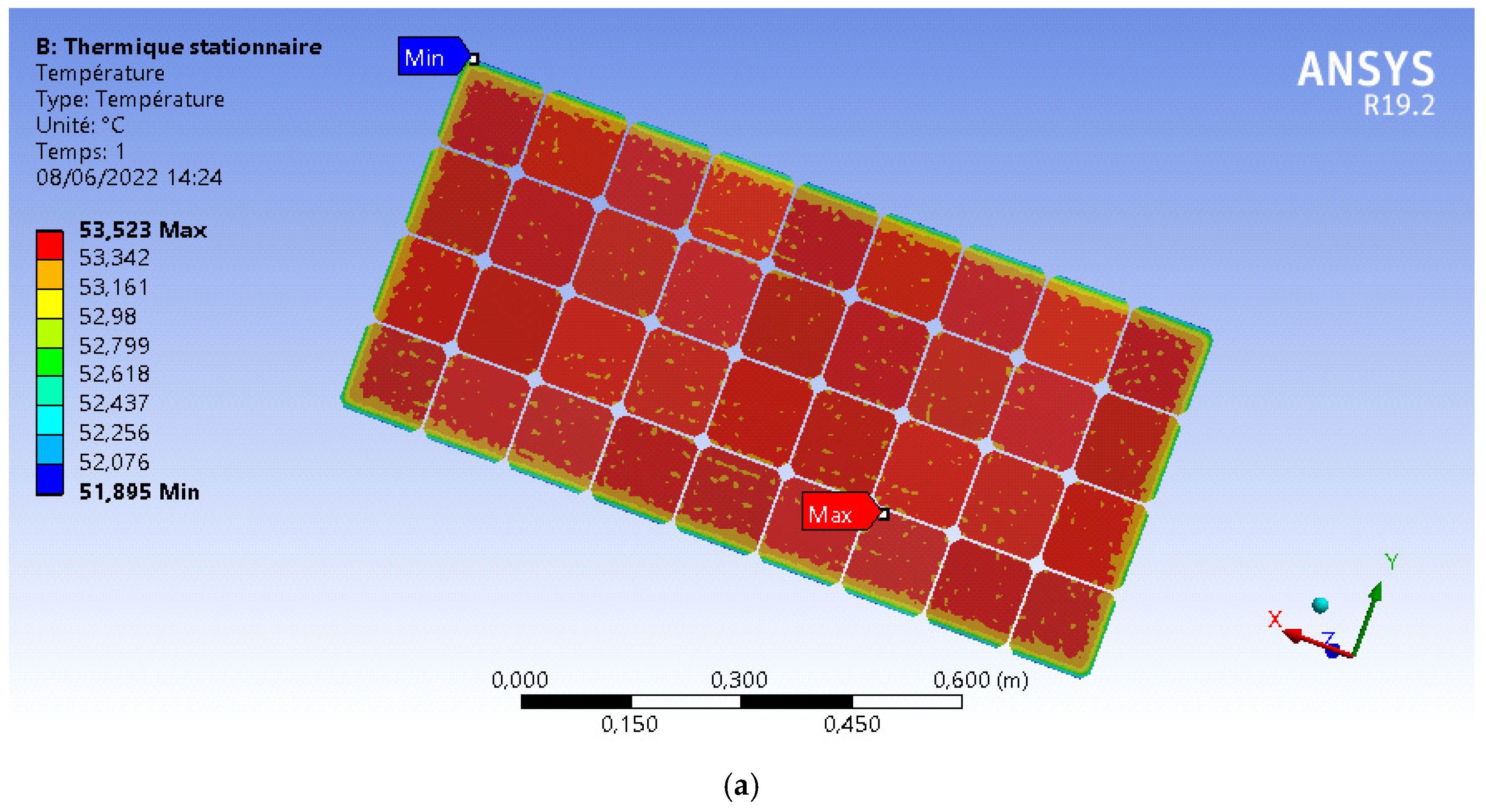
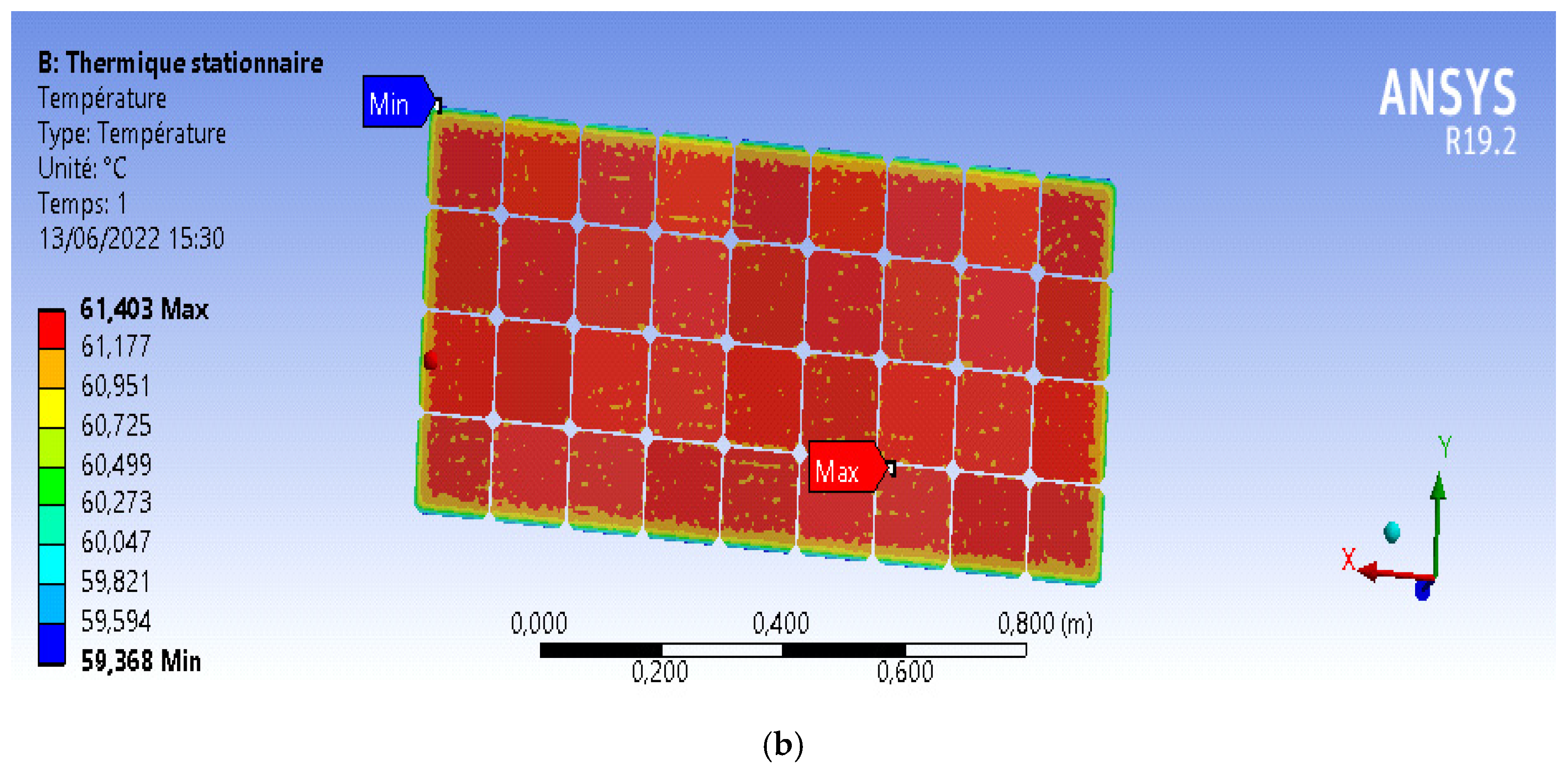
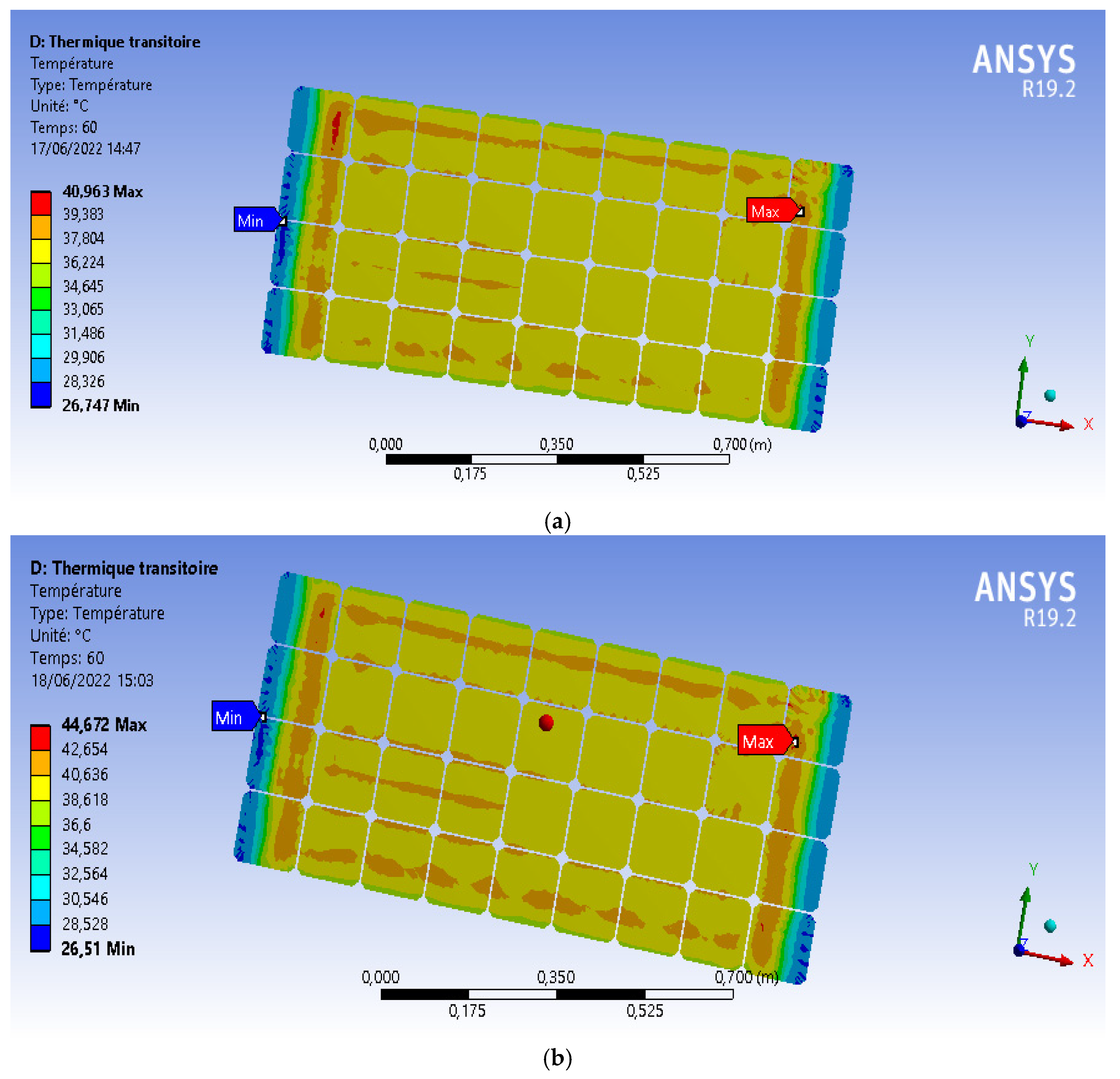
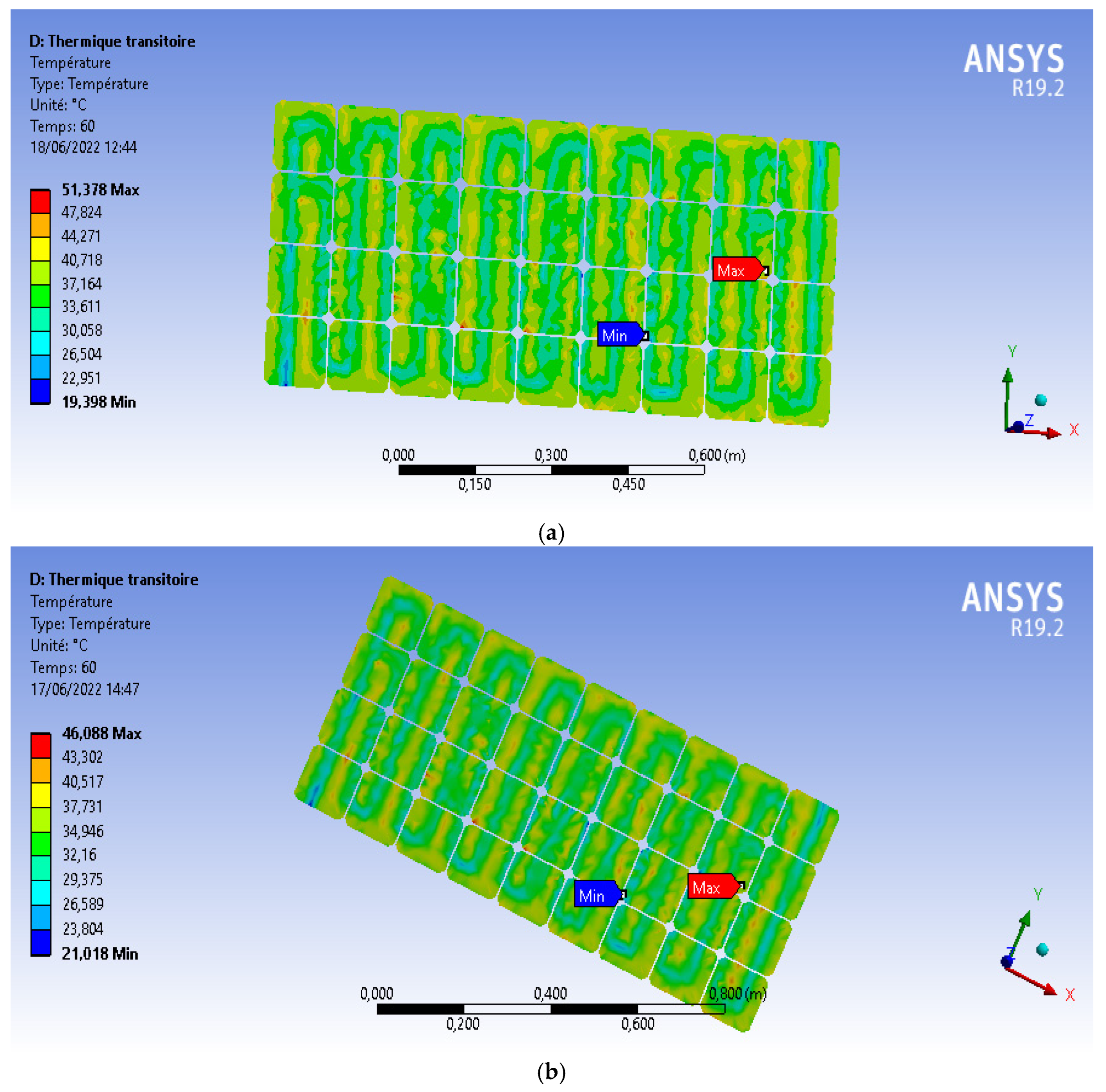
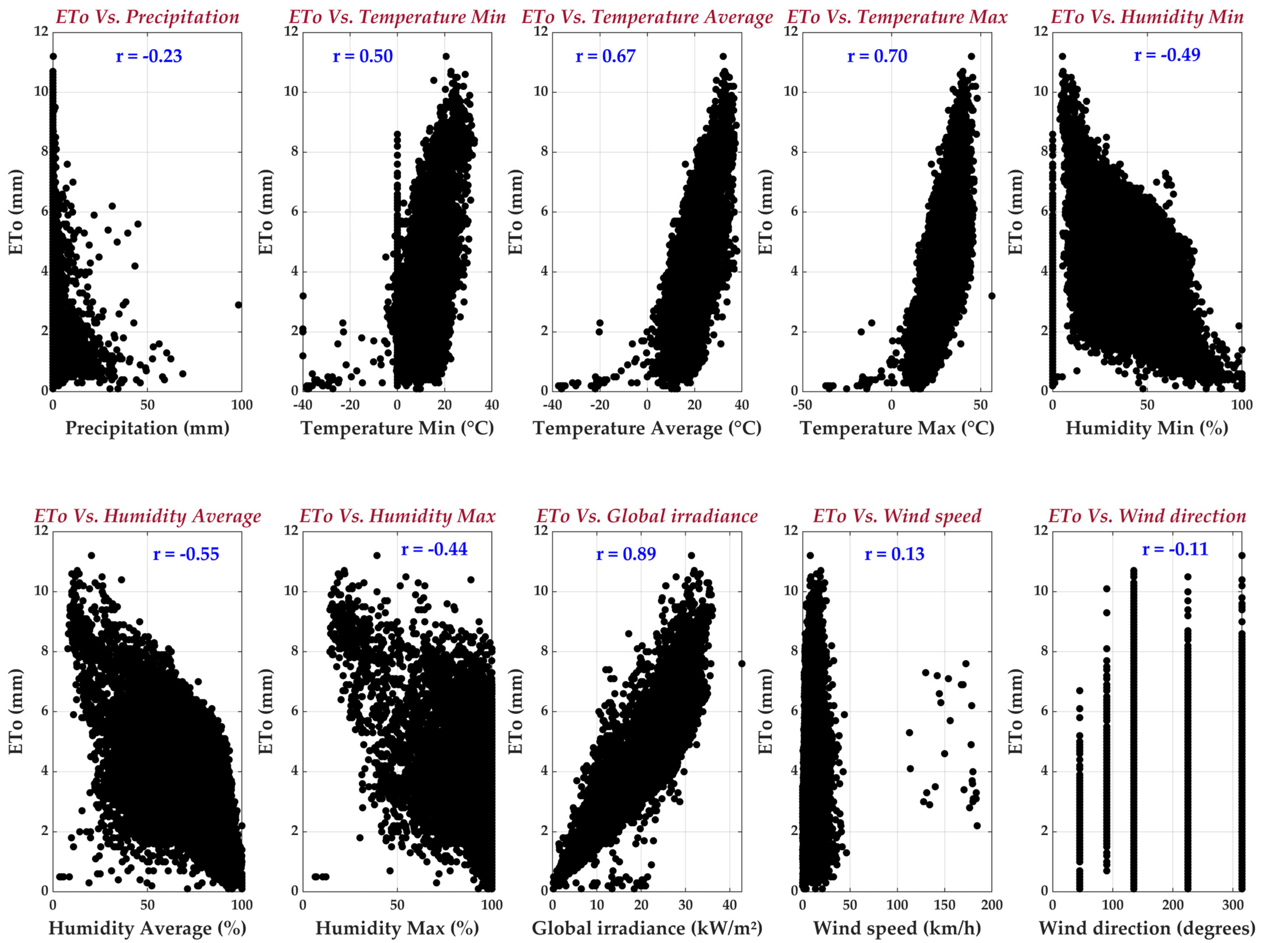
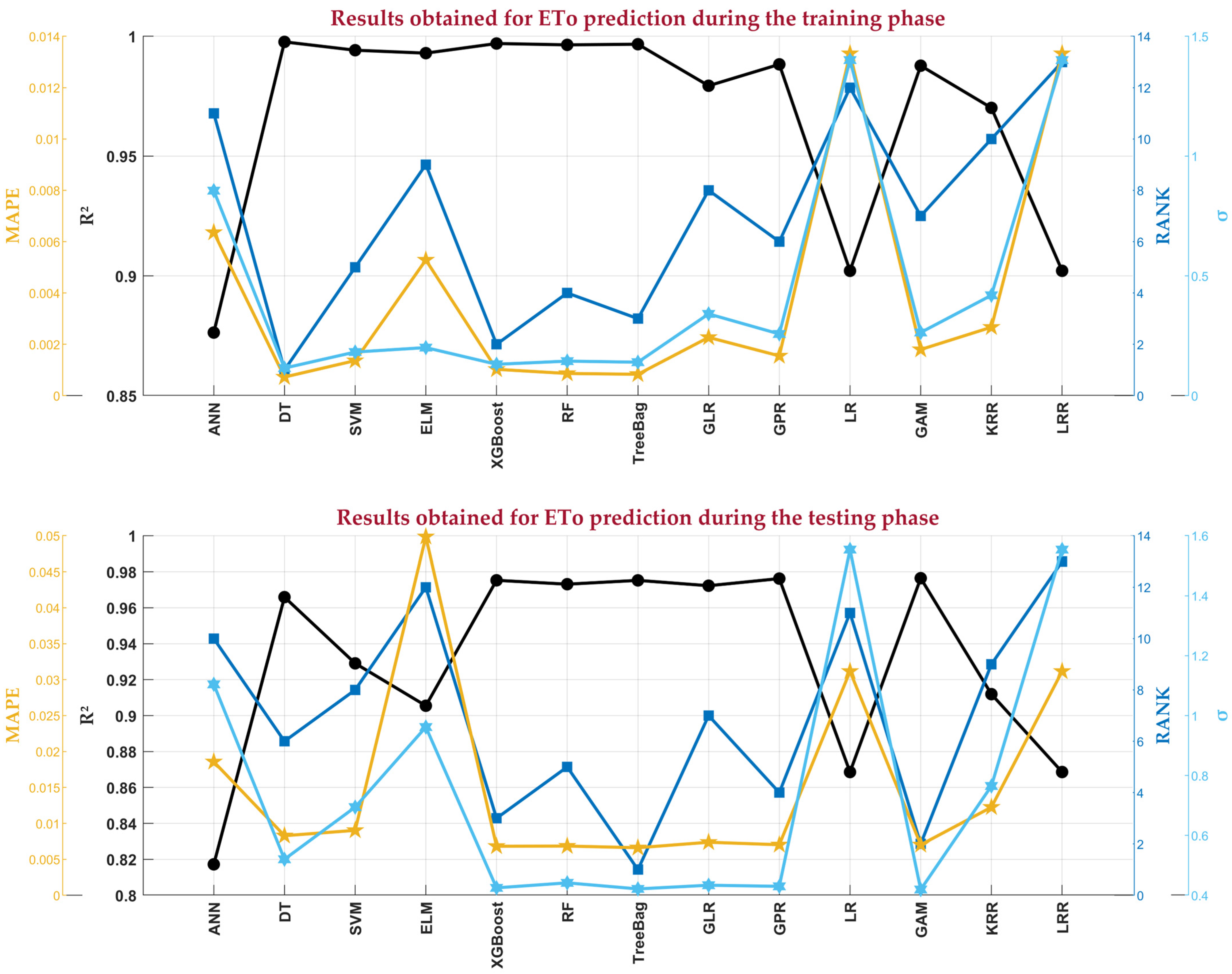

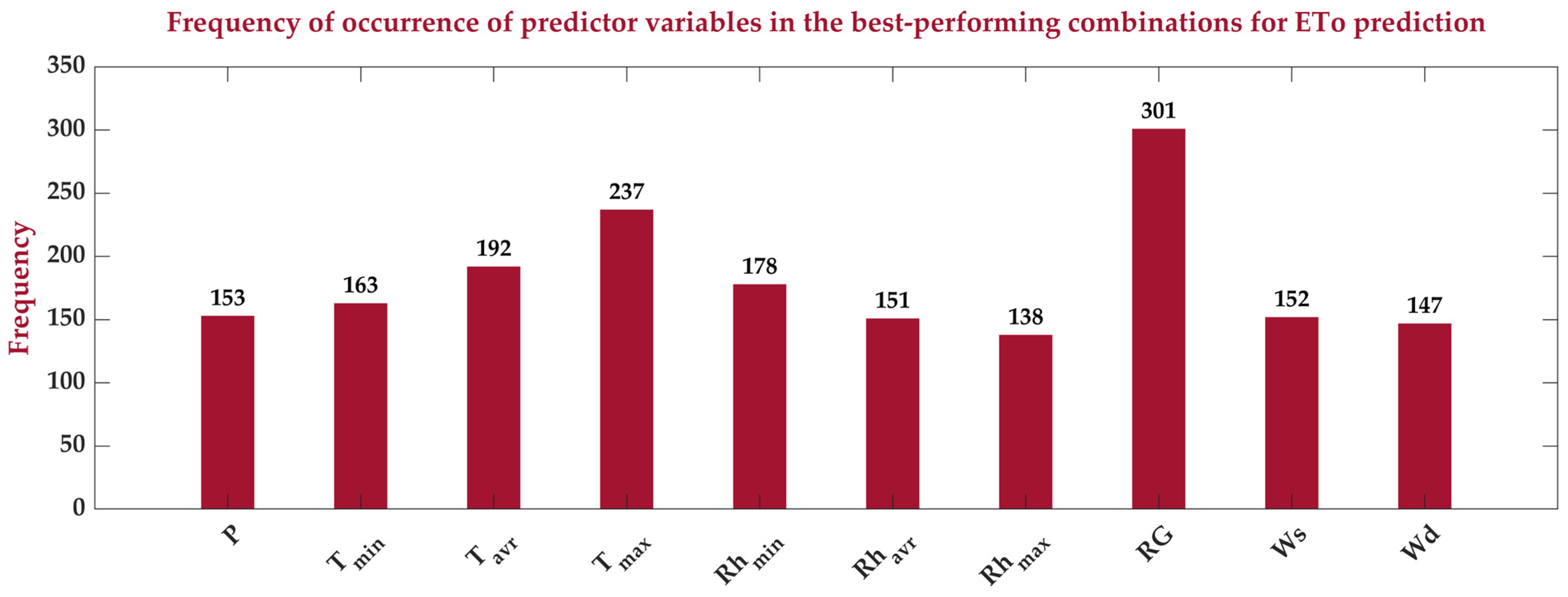
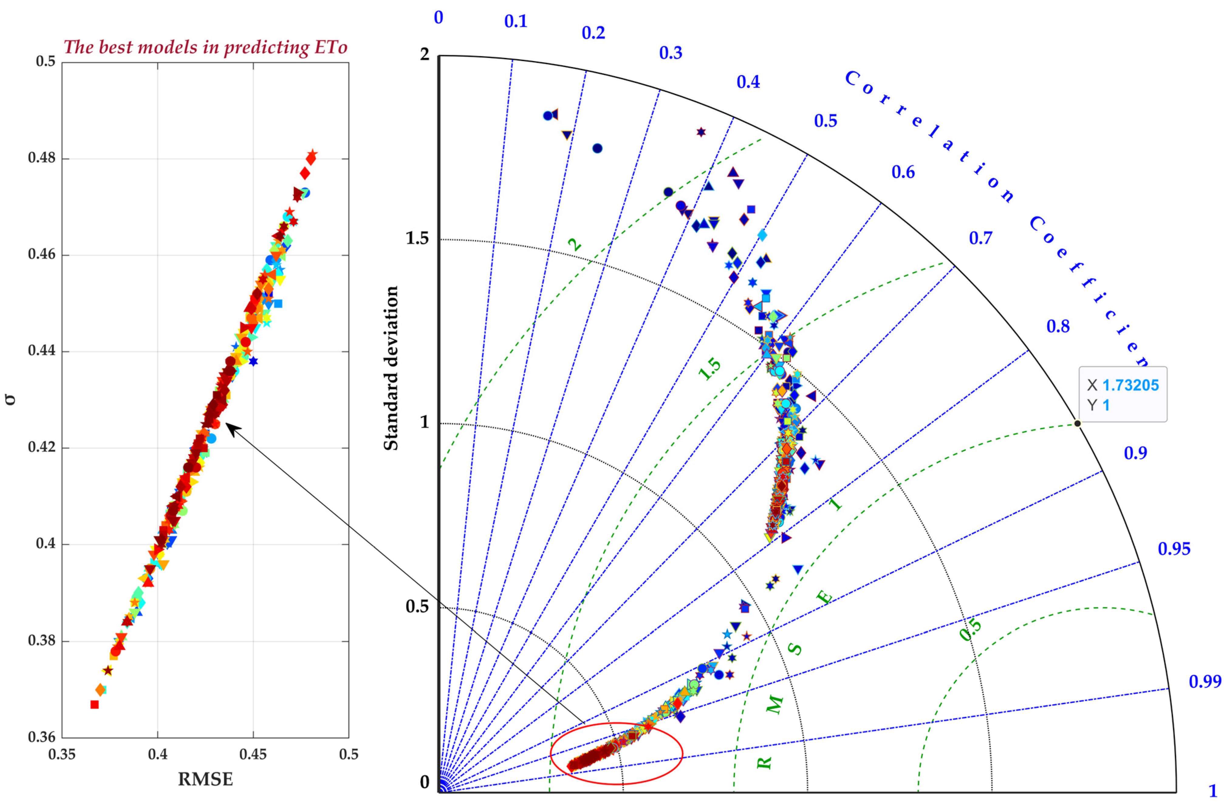
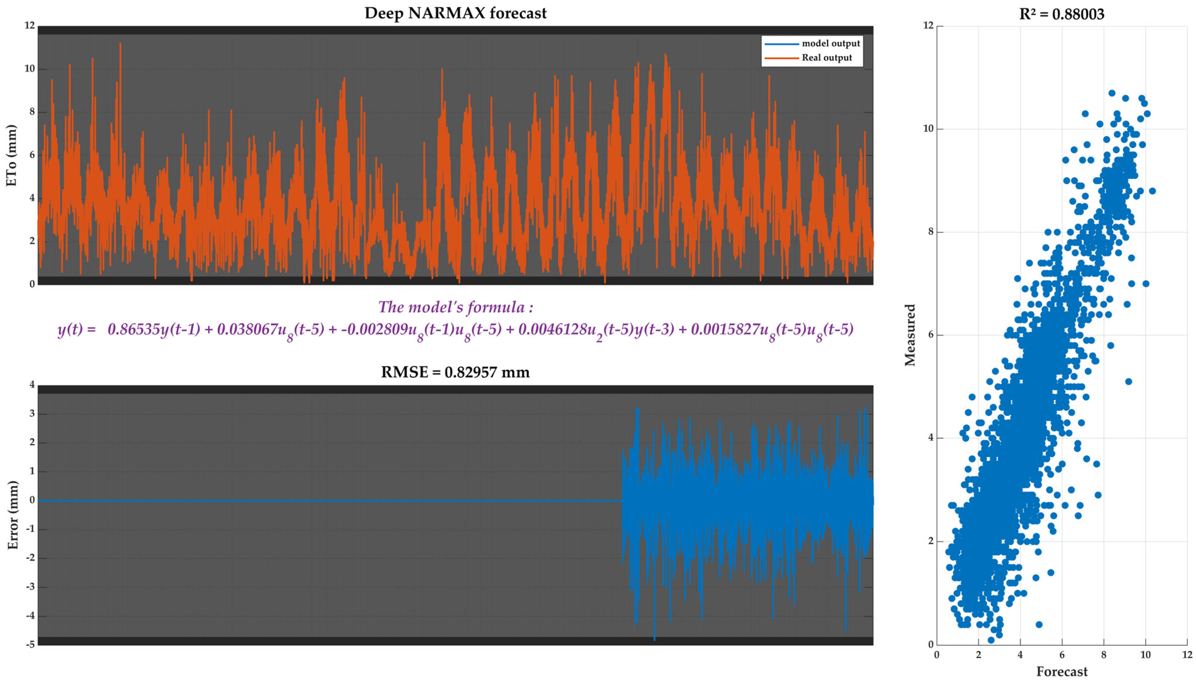
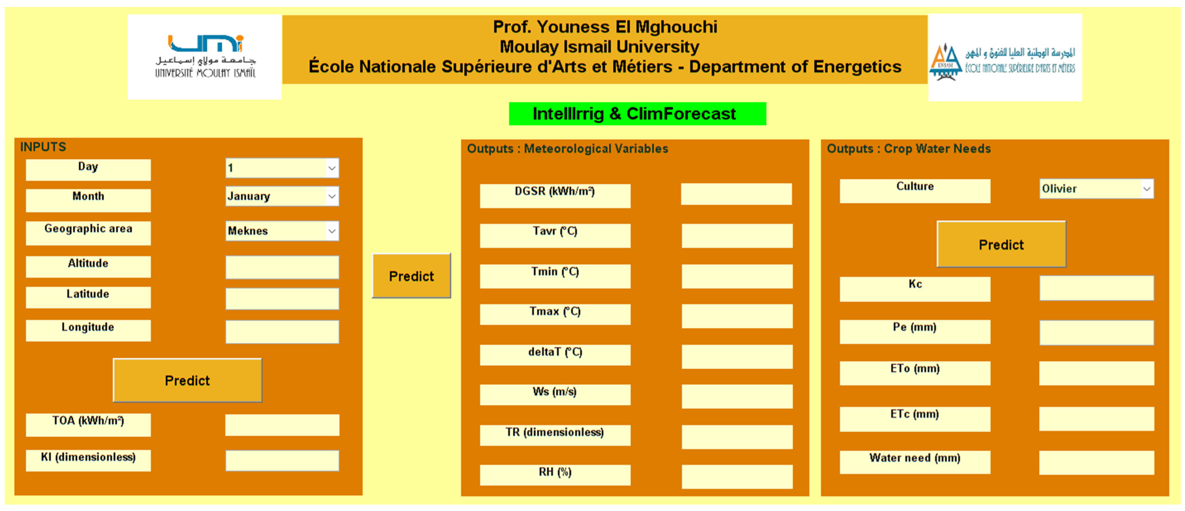
Disclaimer/Publisher’s Note: The statements, opinions and data contained in all publications are solely those of the individual author(s) and contributor(s) and not of MDPI and/or the editor(s). MDPI and/or the editor(s) disclaim responsibility for any injury to people or property resulting from any ideas, methods, instructions or products referred to in the content. |
© 2025 by the authors. Licensee MDPI, Basel, Switzerland. This article is an open access article distributed under the terms and conditions of the Creative Commons Attribution (CC BY) license (https://creativecommons.org/licenses/by/4.0/).