Abstract
The background error variance in variational data assimilation can significantly affect a model’s initial field. Around extreme weather events, the variance of the unbalanced control variables have contributed highly to the total variance. This study investigates the effect of flow-dependent unbalanced variance on tropical cyclone (TC) forecasts using the ensemble of data assimilation (EDA) method. The analysis of TC Saudel (October 2020) shows that flow-dependent unbalanced variances can better represent the uncertainty in the background error, which is investigated in terms of magnitude and distribution. The vertical distribution of the temperature-explained variance ratio also shows that the contribution of the vorticity-balanced variance around Saudel is lower than the global average (in the troposphere). Single-observation experiments reveal that the structured flow-dependent errors of unbalanced control variables can also introduce corresponding structural information in analysis increments. As expected, the experiments in which the variances of all variables are flow-dependent in the one-month TC forecast performed better overall. Compared with the reference, these forecasts reduce the average absolute track and intensity errors by approximately 31% and 9%, respectively. The results demonstrate that EDA-based unbalanced variances can indeed improve the mean forecast skills of TC tracks and intensities despite instability at some lead times by improving the forecast of the circulation situation and providing a more appropriate balance relationship between variables.
1. Introduction
The accuracy of numerical weather prediction (NWP) strongly depends on the initial state, and a good initial state depends on the process of high-quality data assimilation. In a variational data assimilation system [1], the background error covariance matrix ( matrix) plays a crucial role in weighting a priori state, information spreading and smoothing, balance relationship construction, and improving in observation usage efficiency [2]. Therefore, the precise specification of is of great significance for improving the forecasting effect of a model. In practice, the dimension of is vast, and a complete description of the background field error cannot be obtained. It needs to be modeled under appropriate assumptions. Usually, under the assumptions of isotropy, homogeneity, and static conditions, the matrix is implicit in a set of control variable transformations [3,4].
The control variable transformation (CVT) technique converts the objective function minimization of model variables into a functional analysis of control variables, which includes two parts: physical transformation and spatial transformation. The physical transformation expresses the dynamic balance constraint between different variables and transforms the model variables into quasi-independent analysis variables. Generally, the variable that can characterize the main balance pattern of the atmosphere is selected as the first independent analysis variable [5], and the remaining model variables are decomposed into the parts balanced with selected variables and the unbalanced parts. The unbalanced parts are the remaining independent analysis variables. For example, in the European Centre for Medium-Range Weather Forecasts (ECMWF), these analysis variables are vorticity, unbalanced divergence, unbalanced mass (temperature and surface pressure), and specific humidity (considered separately) [6].
The relevant assumptions made for modeling are only a rough approximation of the forecast error. The true error structure must be inhomogeneous and anisotropic and vary with the weather conditions. The wavelet form of the background error covariance model proposed by Fisher [7] enables the matrix to vary with scale and spatial position and considers the inseparability of covariance in the horizontal and vertical directions. Regarding the time-varying characteristics of flow fields, ensemble data assimilation (EDA) can provide flow-dependent estimates of short-term forecast errors with ensemble members and construct a matrix reflecting the uncertainty of the real-time meteorology situation [8,9]. Hybrid data assimilation methods that combine climatological and ensemble covariances have also been implemented and continuously developed in some numerical operational centers (e.g., Met Office and National Centers for Environmental Prediction) [10,11].
The use of EDA to estimate the background error variance of vorticity was implemented in the ECMWF model in May 2011 [12]. Raynaud, et al. [13] used the Arpége system to examine the effect of extending the flow-dependent variance to all variables, emphasizing the importance of correctly representing unbalanced statistics. Bonavita, et al. [14] determined that for temperature and divergence, the variances in unbalanced variables in the control vector that are not constrained by dynamic balance contribute significantly to the total variances, especially for the temperature errors in the troposphere. For high-resolution assimilation systems and particularly areas where quasi-geostrophic theory is less suitable (e.g., the tropics and in extratropical low-pressure systems), the proportion of unbalanced variances further increases.
Tropical cyclones (TCs) are a type of low-pressure system accompanied by high-impact weather and pose a great threat to nearby areas [15]. Currently, the track forecast error of TCs shows a decreasing trend, but the intensity forecast error has not changed much. One of the key factors affecting the intensity forecast is the accurate description of the TC in the initial field of a model [16,17]. Li, et al. [18] studied Hurricane Ike (2008) using the Weather Research and Forecasting (ERF) model hybrid ensemble-three-dimensional variational data assimilation system and found that flow-dependent background errors can dynamically generate more consistent state estimation. Gopalakrishnan and Chandrasekar [19] analyzed the performance of the 4D variational over 3D variational assimilation scheme for the forecasting of two TCs in the Indian Ocean. Previous studies are mostly based on regional models and only focused on specific TC cases. Statistical results on the effect of flow-dependent background error variance on TC forecasting in the global model remain to be evaluated.
The current trend in data assimilation technology is hybrid data assimilation, the key component of which is the use of background error information that can reflect the current flow characteristics. For developing of operational NWP systems, it is important to evaluate the impact of day-to-day background error variance since these results can help guide the design of the assimilation scheme. The improvements in TC forecasting skills also require a flow-dependent description of the background error field. Therefore, it is necessary to analyze the effects of different variables in the flow-dependent control vector (especially the unbalanced components that may play a leading role) on the development of TCs.
The primary purpose of this study is to evaluate the effect of ensemble-based unbalanced variances on assimilation and forecasting and to conduct a detailed analysis on high-impact weather events such as TCs. Specifically, we used the En4DVar assimilation system (Section 2.1) to estimate the flow-dependent background error variances. By comparing the different results of the ensemble estimation only for vorticity and for all control variables, the effect of the flow-dependent unbalanced variances on the TC forecast is obtained. The objectives of this study are summarized as follows: On the one hand, we diagnose the background error variance of the control variables estimated by EDA to verify their flow-dependent characteristics and to inform the further development of the assimilation system (full flow-dependent background error covariance matrix). On the other hand, in the framework of the global model, we analyze the influence of the flow-dependent variance of unbalanced control variables on the track and intensity forecasts of TCs in different regions to preliminarily reveal the role of different control variables and provide possible reasons for improving TC forecasts from a dynamical perspective.
This article is mainly composed of five sections. Section 2 briefly introduces the data assimilation system and forecast model used in this study, the theoretical knowledge of the background error covariance matrix and the related experimental design. Section 3 presents a diagnostic study on TC Saudel, including the comparison of background error statistics under various configurations and the analysis increments of single-observation experiments. In Section 4, the forecast skills are considered. The effects of the unbalanced variances on TC forecasts are investigated through batch comparison experiments and the case study of Saudel. Section 5 provides a summary and discussion of the main conclusions of this study.
2. Experimental Configuration
2.1. Assimilation System and Forecast Model
The assimilation system used in this paper is the Yin-He four-dimensional variational data assimilation system (YH4DVAR), which was developed based on the work of Zhang, et al. [20,21]. It assimilates global meteorological data and provides a high-quality initial field for global medium- and short-term NWP. The system is designed with an integrated cost function, which comprehensively considers the background field, observation processing, gravity wave control, and deviation correction. The model variables are vorticity , divergence , temperature and the logarithm of surface pressure , and specific humidity . As an operational system, YH4DVAR runs the assimilation of global data twice a day, providing a high-precision initial field for the global model. Therefore, the assimilation window was set to 12 h, and the analysis and forecast products of 0000 UTC (1200 UTC) use the observations in the time window from 2100 UTC to 0900 UTC (0900 UTC to 2100 UTC). Approximately 3.5 million observation data points can be assimilated at a single time. These observations have conventional data (humidity, temperature, pressure, and wind) provided by radio sounding, surface, aircraft, etc. Although they are less than 10% of the total, they play an important role in the bias correction process. Most of the observations are unconventional data, such as Advanced Microwave Sounding Unit-A (AMSU-A), advanced technology microwave sounder (ATMS), global positioning system radio occultation (GPSRO), etc., which can detect radiations in the atmospheric column. The radiative transfer model can convert the prior information of the atmosphere into an equivalent amount of atmospheric radiation and compare it with the detection data as the innovations that drive the assimilation system. The current resolution of the system is TL1279L137 (indicating a spectral triangle truncated wavenumber of 1279, a linear grid, and 137 vertical mixed coordinate layers), and the detailed settings of the vertical model levels refer to ECMWF (https://confluence.ecmwf.int/display/UDOC/L137+model+level+definitions (accessed on 20 September 2022)). To improve the computation efficiency, YH4DVAR adopts a multiresolution incremental scheme [22,23] and configures three inner loops (i.e., three minimization iterations). The resolution of the first loop is T159, and the resolutions of the other two are both T255.
The model that matches the assimilation system used in the experiment is the Yin-He Global Spectral Model (YHGSM), which is a global NWP model developed by the College of Meteorology and Oceanography, National University of Defense Technology. The dynamical core of the YHGSM satisfies the dry-mass conservation constraint proposed by Peng, et al. [24]. The time discretization adopts the semi-implicit semi-Lagrangian scheme, and the spatial discretization adopts the spherical harmonic functions expansion (horizontal) and the finite-element method (vertical). For details, see Wu, et al. [25], Yang, et al. [26,27], and Yin, et al. [28,29].
2.2. Background Error Covariance Modelling
The four-dimensional variational (4DVar) cost function in incremental form can be expressed as:
In the actual algorithm implementation, the variable transformation matrix is used to transform the model variables from the incremental space to the control vector space [4,5], which can be expressed as:
The control vector is the vector processed by the minimization algorithm in the assimilation system. The analysis field is the model variable field when the cost function is optimal. The difference between the analysis field and the background field is expressed using the analysis increment , i.e., . The subscript is the time index corresponding to the observation, and is the priori estimate (background field) of the target atmospheric state analysis field . is the innovation vector, is the observation vector, is the observation operator that maps the model variables to the observation space, and is obtained by the linearization of the observation operator near the background state. represents the state field corresponding to the background field propagating to time through the complete nonlinear model, and represents the state where the control vector at the initial time propagates through the tangent linear model to time . is the observation error covariance matrix. The background error covariance matrix does not appear in Equation (1) but is implicitly represented by the matrix ().
YH4DVAR uses a spherical wavelet background error covariance model [7,30], and the corresponding CVT relationship based on a spherical wavelet is:
where represent wavelets of different scales, is the vertical covariance matrix on the wavelet space and the horizontal position ( is longitude, is latitude), is the wavelet control variable, stands for convolution, is the wavelet transform, is the background error variance in the grid space, and represents the balance constraint relationship between different variables.
The control variable transformation matrix usually includes balance transformation and spatial transformation. Balance transformation deals with the correlations between different variables. The original background error covariance matrix is transformed into a diagonal matrix by balance transformation, so that those independent analysis variables can be considered separately. Thus, the original multivariate problem is transformed into a univariate problem [31]. Spatial transformation deals with the spatial correlation of the same variable. In the YH4DVAR system, vorticity, as a variable that characterizes the main balance mode of the atmosphere, is called a balanced variable. The remaining variables are decomposed into balanced parts and unbalanced parts by the balance operator. This process can be represented in matrix form:
where the first matrix on the right is the balance operator matrix , represents the correlation between the divergence increment and the vorticity increment, and represent the balance between the mass field and the wind field [4,7,32]. These matrices are estimated with the National Meteorological Centre (NMC) method and using linear regression for calibration [33]. The second matrix on the right consists of the control variables, which are vorticity , unbalanced divergence , unbalanced mass , and specific humidity . The model variables on the left side of the equation are correlated, and through the balance operator, the control variables on the right are independent of each other, which can be considered separately.
2.3. Flow-Dependent Estimation and Postprocessing of Variances
The data assimilation system used in this work mainly includes an EDA cycle and a deterministic 4DVar cycle. The flow-dependent background error variances were estimated from the EDA cycle. First, the background field, observation data, and sea surface temperature (SST) field were perturbed. The perturbation of the background was implemented implicitly by perturbing the physical process tendency in the numerical prediction model. The perturbations of observation and SST were achieved by superimposing random noises obeying their respective error distributions. Then, the perturbations were input into the EDA cycle to obtain the perturbed analysis fields, and the forecast field (background field) ensemble was obtained through the forward integration of the forecast model. Next, the raw variances estimated from the ensemble samples were scaled and filtered to obtain the EDA variances. Finally, the background error variances with flow-dependent properties were used as the input of the deterministic 4DVar cycle (only used in the minimization step). To reduce the computational cost, the resolution of EDA is usually lower than that of the 4DVar cycle. In the EDA cycle, two layers of inner loops were used with resolutions T95 and T159, respectively, and one layer of outer loops had a resolution of T399. In the deterministic 4DVar cycle, three layers of inner loops (T159/T255/T255) and one layer of outer loops (T1279) were used. Similar configurations can also be seen in the ECMWF operational system [9].
Using ensembles to estimate the flow-dependent background error variance, one of the key points is to select the appropriate number of members. Sampling noise considerably affects the accuracy of estimation. Pereira and Berre [34] noted that the accuracy of variance estimation based on EDA is directly proportional to the root mean square of the number of ensemble members. Increasing the size of the ensemble is beneficial, but it also brings a significant increase in the amount of computation. Due to the limitation of computation cost and the demand for the timeliness, the operational number of members is on the order of . Several studies have focused on the impact of finite-size ensemble samples [35,36,37,38]. Bonavita, et al. [39] showed that a relatively small set (e.g., 10 members) can adequately characterize the large-scale error structure of extratropical cyclones, and a larger set can model more refined features. The research of Liu, et al. [40] found that the variance estimation using 10 members is very similar to the 30 members except for the relative reduction in noise, and there is no essential difference between the two. The number of EDA members in this article is also taken as 10.
To reduce the effect of random errors, an objective filtering method [41] with a small amount of calculation was used in the process of variance postprocessing. The estimated variances were filtered using the following spectral low-pass filter:
where is the wavenumber, is the truncation wavenumber (i.e., the corresponding wavenumber when the signal energy spectrum is equivalent to the random sampling noise variance energy spectrum), and is the spectral filter coefficient. The filtering process converts the ensemble-estimated variance in the grid space to the spectral space and multiplies it by the filter coefficient so that the larger-scale signal passes through and the smaller-scale noise is filtered out.
2.4. Experimental Design
In the operational YH4DVAR system, the variances at each analysis time are first calculated from the 10-member EDA (lower resolution) and then applied to the operational 4DVar. Among all the control variables, the analysis of specific humidity is independent and not related to other variables and is not considered. In addition, this study only focuses on the flow-dependent variances, and the correlations (i.e., off-diagonal elements of ) are climatological.
The objective of experiments is to evaluate the effect of flow-dependent variances of unbalanced control variables (i.e., unbalanced divergence, unbalanced temperature, and surface pressure). Therefore, we performed three experiments. In the vorticity-balanced flow-dependent variance experiment, the variance in vorticity is calculated from the EDA, while the remaining part of the control vector is derived from the climatological statistics. As the equations in Section 2.1 indicate, vorticity plays a crucial role in describing the balanced relationship among different variables. The flow dependence of vorticity variances can be projected to the balanced parts of divergence, temperature, and surface pressure through the balance operator. Therefore, we call this experiment “flow-dependent balanced”, abbreviated as “fbal”. A fully flow-dependent description of variances is investigated in the second experiment, which means that the variances of all control variables are provided by the ensembles. By comparing with “fbal”, we can determine the effect of variance of unbalanced variables. The second experiment is abbreviated as “fall”. As a reference, we also ran a control experiment (abbreviated “ctrl”). In this experiment, the variances of all control variables are static and derived from climatology.
One-month assimilation/forecast experiments with three conditions were run in October 2020 (0000UTC 01 to 1200UTC 31). The assimilated observations include surface observations, aircraft data, sea surface observations (e.g., drifting buoys and ship reports), in situ sounding data, wind profiler radar data, global positioning system radio occultation bending angle, and radiances from polar-orbiting satellites (e.g., AMSU-A, MHS). The observations are subjected to various quality check steps, such as bias correction, variational quality control, and thinning before entering the assimilation system.
3. Diagnosing the Background Errors
To evaluate the expected impacts of the flow-dependent variances in unbalanced control variables, we compare the distributions of the background error standard deviations and analysis increments of different variables under various experimental configurations. The comparisons focus on the full variables instead of the control variables [13].
3.1. Distribution of Background Error Standard Deviations
Provided here is the distribution of the standard deviations of the different variables in the one-month comparative experiment described in Section 2.4. First, vorticity, which determines the balanced parts of the flow in the mass-wind balance formulation, is analyzed. Figure 1 displays the standard deviations of vorticity near 850 hPa in a limited area (spatial range: 0° to 30° N, 110° to 140° E) for two dates (1200 UTC 19 and 0000 UTC 20 October 2020). The low-value area of the geopotential height is related to TC Saudel, which caused severe flood damage when passing through the Philippines. In flow-dependent variance maps, the area near Saudel exhibits a high standard deviation value. EDA predicts a large vorticity spread zone corresponding to the 850 hPa situation field, and the position of the TC is identified. Comparing Figure 1B,D, we also find that the magnitude and structure of the enhanced EDA spread vary with the intensity of Saudel. At 1200 UTC on 19 October 2020, Saudel is a tropical depression with a loose structure. After 12 h, the strengthened TC has a more complete and concentrated structure. Thus, the standard deviation in Figure 1D is higher and more concentrated than that in Figure 1B. At the same time, the area of increased uncertainty changes with the position of Saudel, which is identified by the geopotential height contour. However, the flow dependence cannot be seen in the control experiment. The background error estimation derived from the climatology is approximately flat, and there is no obvious high-value center, which can hardly reflect the uncertainty of the existence of the TC. The global distribution of the variable standard deviation (not shown) also shows the above characteristics. The EDA spread has obvious anisotropy and is closely related to the flow field.
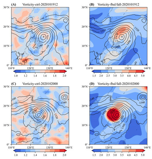
Figure 1.
Standard deviations of vorticity at model level 114 (~850 hPa) at times 1200 UTC 19 October 2020 (top panel) and 0000 UTC 20 October 2020 (bottom panel). The left column (A,C) refers to the control experiment, and the right column (B,D) refers to the flow-dependent experiment. Unit: s−1. The corresponding 850 hPa geopotential height analysis is overlaid, contour: 10 dagpm.
Furthermore, the contributions of the unbalanced background error statistics are investigated in terms of surface pressure and temperature. That is, we separately evaluate the contributions of variances in the vorticity-balanced term and unbalanced components to the total variances.
Standard deviation maps of the logarithm of surface pressure are shown in Figure 2. Figure 2B shows that the flow-dependent vorticity-balanced standard deviation can identify the increased uncertainty information corresponding to Saudel. In this dynamically active area, the vorticity-balanced variance accounts for approximately 65% of the total variance. The distribution of unbalanced standard deviation (Figure 2A) also shows a connection with the flow. The high-value area is approximately distributed along the contour of the geopotential height. In conjunction with Figure 2C, we can see that in the tropical convection area, the EDA-based unbalanced variance can enhance the flow dependence of the total variance, corresponding to a more obvious high standard deviation area and a more detailed structure, which can better describe the uncertainty in the forecast error.
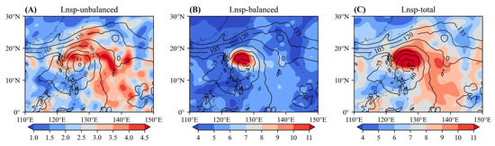
Figure 2.
Standard deviations of the logarithm of surface pressure in the fully flow-dependent experiment corresponding to 1200 UTC 19 October 2020. The total standard deviations (C) are decomposed into vorticity-balanced parts (B) and residual unbalanced parts (A). Unit: hPa. The corresponding 1000 hPa geopotential height analysis is overlaid, contour: 15 dagpm.
The average amount of explained variance [6] between the global and local ( area centered on Saudel) is calculated. For surface pressure, the global average explained variance ratio can reach 70%, which is higher than that in the area around Saudel (65%). This means that the contribution of unbalanced variance to total variance increases in the vicinity of Saudel. However, regardless of the global scope or the region of TCs, the vorticity-balanced part plays a major role. Based on the dominance of the main balance variable, it is necessary to use EDA to estimate the vorticity variance. Figure 3 illustrates the vertical distribution of the temperature-explained variance for the global average and around Saudel at 1200 UTC on 19 October 2020. The variances of unbalanced components play an important contribution to the total variances of temperature error, especially in the area around Saudel in the troposphere. Due to the existence of Saudel, the unbalanced error is relatively large below model level 60 (~100 hPa), and the temperature is more weakly explained by vorticity. In the area above model level 60, the proportion of explained variance increases. This can be explained by the fact that in the geostrophic adjustment of the area near the equator, the mass field is adjusted to the rotating wind field, and the rotating wind (such as vorticity) represents the main balance mode [5]. The ratio near the stratopause (above model level 20) is relatively small because this is the area where the mass-wind balance is least effective.
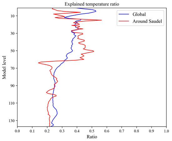
Figure 3.
Vertical profiles of the ratio of the total temperature variance that is explained by vorticity for the global average (blue line) and around Saudel (red line) at 1200 UTC 19 October 2020.
The above results all indicate the important contribution of the EDA-based variances of the unbalanced variables in the vicinity of TC. The introduction of the flow-dependent unbalanced variance affects the magnitude and structure of the total variance. It can be expected that, due to the various structures of background errors, the same observation located close to this area has distinct effects on analysis and forecasting.
3.2. Analysis Increments of Single Observations
The effect of unbalanced variances on deterministic 4DVar analysis is investigated through a single-observation trial. The assimilation time window of the trial is set to 0900 UTC–2100 UTC on 19 October 2020. At the beginning of the assimilation window, a single temperature observation with a departure near the center of Saudel (15.5° N, 130° E at 1 km) is used. Since the background field is provided by the previous forecast, this is a warm start, and the same settings are used for the three experiments (Section 2.4).
Figure 4 presents geographical maps of the temperature analysis increments near 700 hPa at the beginning of the assimilation window. A clear difference observed is the magnitude of the analysis increment. In the “ctrl”, “fbal”, and “fall” experiments, the maximum temperature increments are 0.006 K, 0.009 K, and 0.012 K, respectively. The flow dependence of unbalanced variances can enhance the uncertainty of the background error estimate, and it is further reflected in the analysis increment (comparing Figure 4B,C). In addition, although the increment is mainly distributed near the observation position, in the EDA-estimated variance experiments, the shape of the increment shows a shift to the TC center, especially in the “fall” map. This reflects the propagation of observation information to the surroundings under background error modulation. Figure 5 shows the zonal cross-section of the vorticity analysis increment at 15 °N below model level 80. The same feature also appears in the vertical distribution of the vorticity increment. The three experiments all show obvious maximum and minimum centers in the vertical direction, but the value of the “fall” experiment is the largest, which corresponds to the more significant divergence and convergence of the upper and lower airflows (this emphasizes the contribution of unbalanced divergence and mass variances). Meanwhile, although the extremum range of the EDA experiment is more extensive (vertical extension), the “ctrl” experiment also shows expected anisotropic characteristics corresponding to the weather event. This flow dependence may originate from the balance operator and/or the dynamic constraints of the model.
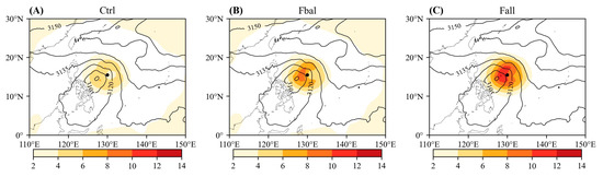
Figure 4.
Single observation analysis increments for temperature at model level 105 (~700 hPa) valid on 19 October 2020, 0900 UTC. (A–C) correspond to the “ctrl”, “fbal” and “fall” experiments, respectively. Unit: K. The corresponding 700 hPa geopotential height analysis is overlaid, contour: 15 gpm. The black dot shows the observation position.
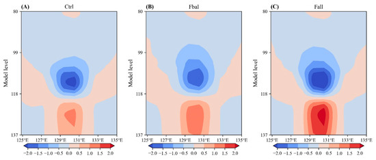
Figure 5.
Zonal cross-section of vorticity analysis increment in the model level 80–137 at 15° N valid on 19 October 2020, 0900 UTC. (A–C) correspond to the “ctrl”, “fbal” and “fall” experiments, respectively. Unit: s−1.
4. Effects of Flow-Dependent Unbalanced Variances on the Forecast
The single-observation results show that the introduction of the variances of flow-dependent unbalanced variables can propagate the observation information to a more uncertain area and ultimately result in a different incremental structure. It can be determined that different increments have other effects on the subsequent forecast. In this section, these effects are evaluated through several TC cases in October 2020.
4.1. Case Study of Saudel
On 18 October 2020, a tropical depression formed in the Philippine Sea and moved northwest. Saudel developed on 20 October and intensified into a tropical storm (landing in eastern Luzon) on the same day. Saudel left the Philippines as a typhoon on 22 October and moved toward Vietnam. It began to weaken on 25 October and eventually dissipated before making landfall. To preliminarily assess the possible impact on Saudel, we choose the forecast results at 0000 UTC on 20 October 2020 in the comparative experiments (Section 2.4). The forecast time is from 0000 UTC on 20 October 2020, to 1800 UTC on 25 October 2020, with an interval of once every 6 h. The forecast data of TCs, such as vortex center position and minimum mean sea level pressure, are objectively analyzed by the Geophysical Fluid Dynamics Laboratory (GFDL) vortex tracker program [42]. The TC best track data (version 4) of the International Best Track Archive for Climate Stewardship (IBTrACS) [43] are used as observations.
Figure 6 illustrates the track and corresponding errors of Saudel under various configurations. The overall trend of Saudel is simulated in all three experiments (Figure 6A), and the errors both show an increase with the extension of the integration time (Figure 6B). Compared with the reference run, EDA can significantly improve the forecast skill, especially in the full flow-dependent variance experiment: both the analysis field (0 h) and the forecast field show better results, and the 24 h and 48 h position errors are reduced to less than 15 km.
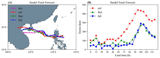
Figure 6.
Tracks of Saudel (A) and corresponding track errors (B) compared with the IBTrACS best track data. Three forecasts from the “ctrl”, “fbal”, and “fall” runs with the initial time at 0000 UTC on 20 October 2020.
The results of Saudel intensity forecasts are presented in Figure 7. The minimum mean sea level pressure (MSLP) gradually decreased with the development of Saudel over the first 72 h and reached its lowest value on approximately the third day, after which the TC weakened and the pressure increased. The control experiment simulates the further strengthening process of the TC after 36 h, while the experiments that introduce flow-dependent information show that the intensity forecast is weaker (higher MSLP). However, the time evolution of the errors (Figure 7B) reveals that except for 48 h to 72 h, the MSLP of EDA is close to the observation. The average absolute errors of “ctrl”, “fbal”, and “fall” are 6.67 hPa, 6.28 hPa, and 5.84 hPa, respectively, which reflect the positive impact of the flow-dependent unbalanced variance on the overall intensity forecast.
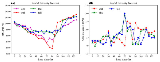
Figure 7.
Similar to Figure 6 but for intensity forecast, (A) is the forecast results of different time periods, and (B) is the corresponding errors. The intensity of Saudel is identified by the minimum mean sea level pressure (MSLP), and the absolute error is equal to the absolute value of the difference between the forecast and the observation.
For unbalanced control variables, the impact of the day-to-day variance estimated by the ensembles and the static variance randomly sampled from the climatological matrix on the total variable variance is achieved through the balance relationship. Thus, we calculated the wind–pressure relationship in Saudel’s forecast (between maximum 10 m winds (Vmax) and minimum MSLP, Figure 8). Without considering the observation error, the observation line represents the true wind–pressure relationship. The closer the lines of different experimental schemes are to the observed values, the better the results. It can be seen that the wind–pressure balance predicted by the “fall” run is closer to the observation. A more realistic balance relationship can effectively transfer the error information of the unbalanced control variables to the model variables, and then affect the analysis increments. When the MSLP is 968 hPa, the observed Vmax is 43.4 m s−1, and the corresponding values predicted by “ctrl”, “fbal”, and “fall” are 33.5 m s−1, 34.0 m s−1, and 36.4 m s−1, respectively. This may be one of the reasons for the track improvement, that is, the track improvement is due to improved storm speed forecasts.
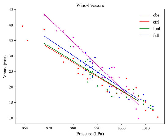
Figure 8.
Relationship between maximum 10 m winds (Vmax) and minimum mean sea level pressure (MSLP); the initial forecast time is 0000 UTC on 20 October 2020.
4.2. Further Verification
We further investigated the forecasts of Saudel at different initial times and the effects of different TC cases that appeared in the North Atlantic (NA) and Western Pacific (WP) during the same period (Table 1). The results of three forecast runs (“ctrl”, “fbal” and “fall”) were also analyzed by the GFDL vortex tracker program and then compared with the best track data of the IBTrACS.

Table 1.
List of TCs used in experiments. One forecast is made at 0000 UTC every day. The North Atlantic and West Pacific are abbreviated as NA and WP, respectively.
To analyze the effect on each TC forecast, Table 2 shows the position and intensity error averaged for different initial and forecast times. Figure 9 and Figure 10 also show the error change in each TC. The longest forecast time of experiments is set to 6 days (144 h), but due to different TC lifetimes, there are differences in the lead time shown in the Figures. EDA has a positive effect on the track and intensity forecast (except during 48–72 h) of Saudel at different initial times, especially for the full flow-dependent variance experiment. The case of a strong typhoon during the same period, Molave, shows a more obvious improvement effect in the “fall” run. The flow-dependent unbalanced variance may have a higher contribution to strong TCs since a stronger TC corresponds to greater uncertainty in the background errors. However, the strong typhoon in the NA has no similar good effects, especially for the MSLP forecast. This illustrates the difference in the contribution of flow-dependent variances, even though they are also tropical. The results of Delta, also located in the NA, show that the position (intensity) forecast of the “fall” run before 54 h (78 h) has the best skill, but as the forecast time increases, its effect decreases faster. We consider that dynamical adjustment may occur when using the EDA-based unbalanced variances, so the forecast of “fall” is not as effective as “fbal” for the track of Delta (Table 2).
Table 2.
Track and intensity errors average for each TC. Intensity errors are based on the minimum mean sea level pressure (MSLP). Absolute errors are the absolute value of forecast-minus-observation.
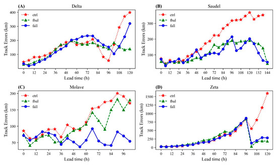
Figure 9.
Track errors of Delta (A), Saudel (B), Molave (C), and Zeta (D) averaged for different initial forecast times.
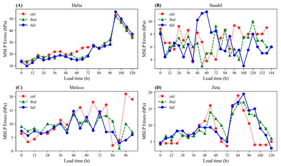
Figure 10.
Intensity (MSLP) errors of Delta (A), Saudel (B), Molave (C), and Zeta (D) averaged for different initial fore-cast times.
The average forecast errors of the three experiments are shown in Table 3. The “fall” run has minimal track and intensity errors. Compared with the “ctrl” run, the “fall” run reduces the average absolute track and intensity errors by approximately 31% and 9%, respectively. One of the main factors affecting the TC track is the large-scale environmental guidance flow. The forecast scores (Anomaly Correlation Coefficient (ACC)) and root mean square errors of 500 hPa geopotential height in tropical areas (Figure 11) averaged for October 2020 both show the positive effect of full flow-dependent variances. This may explain the improvement in the track forecast effect. It is worth mentioning that introducing only the flow-dependent vorticity variance seems to have a significant improvement effect for the TC position (compare “ctrl” and “fbal”) but not for the intensity. This means that the unbalanced variance may play a more important role in the intensity prediction of TC.
Table 3.
Average track and intensity errors of all forecasts from three experiments.
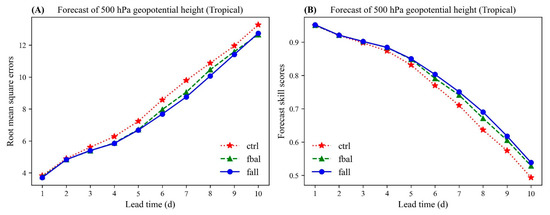
Figure 11.
Root mean square errors (A) and forecast skill scores (B) of geopotential height forecasts at 500 hPa. Scores and errors are averaged over the period 1–31 October 2020 for tropical regions.
5. Conclusions and Discussion
Accurate representation of background error variance considerably affects the forecast performance of variational data assimilation systems for TCs. In this work, an EDA system was used to estimate the day-to-day variances, and three experiments (ensemble estimates for all control variables, vorticity only, and climatological estimates for all variables) were investigated to examine the effects.
The mechanism by which flow-dependent variances affect analysis was investigated through a single-observation experiment and a case study analysis for TC Saudel. The introduction of flow-dependent unbalanced variances can further strengthen the connection with the underlying flow and can describe the background error characteristics in more detail. They can make better use of the observations, that is, provide larger weight to observations near areas of enhanced uncertainties in the analysis. For active dynamical areas, such as that affected by TC, the contribution of the unbalanced background error variances to the total variances is higher for mass variables. The use of EDA variances of unbalanced variables also propagates flow-dependent information into the analysis increments, indicated by the anisotropic increments of Saudel. It is expected that the analysis will be further improved once the flow-dependent correlation information is used. Statistical results of a series of TC forecasting experiments verify the advantage of the full flow-dependent of control variable variances. Although there are differences across time, region, and TC, the EDA-based unbalanced variances can improve overall track and intensity forecasts. The track and intensity of TCs are determined by a combination of external forcing (e.g., guidance of large-scale circulation, the influence of approaching cyclones, etc.) and internal dynamical factors (e.g., convective asymmetry, vertical coupling of high and low-level vortices, etc.). The increase in the 500 hPa geopotential height forecast scores and the more realistic wind–pressure balance relationship indicates that the improved large-scale circulation forecast and the description of the dynamic balance between different variables are responsible for the improvement of track forecasting. Nevertheless, the global system’s description of the TC internal dynamics may not be fully accurate (due to resolution limitations), resulting in less pronounced intensity improvements than the track. Although more in-depth analysis is needed, these results are valuable in guiding the design of operational assimilation systems.
Furthermore, we found that the two experiments that introduced flow-dependent information did not accurately predict the strongest magnitude and temporal evolution of the ‘Saudel’ intensity (Figure 7). To analyze whether it is the effect of the number of ensemble members, a single forecast for Saudel was performed using a 20-member ensemble (similar to Section 4.1). However, increasing the ensemble members did not significantly improve the results (not shown). Next, we will diagnose these failed cases and identify possible causes to further improve the system. There are also some fluctuations in the “fall” experiment for different TC cases. It is worth analyzing the reasons for the different effects of different cases. Is it related to the intensity scale of the TC itself or the external environmental factors (e.g., sea surface temperature)?
We only assessed the effect of the variance of control variables, the correlation is also an important part of the background error covariance. A covariance model with full flow dependence needs to be evaluated to investigate the combined effect of flow-dependent variance and correlation. Finally, the main disadvantage of En4DVar is its high computational cost. Whether the gradient descent information (such as direction) of the previous member can be used to accelerate the solution algorithm of the next member based on the similarity of the minimization process of each ensemble member is also a direction worthy of further exploration.
Author Contributions
Conceptualization, W.Z. (Wei Zhang) and B.L.; methodology, W.Z. (Weimin Zhang); validation, S.L., X.C. and X.X.; formal analysis, S.L.; writing—original draft preparation, W.Z. (Wei Zhang); writing—review and editing, B.L. and S.L.; visualization, W.Z. (Wei Zhang). All authors have read and agreed to the published version of the manuscript.
Funding
This research was funded by the National Natural Science Foundation of China, grant number 42005003.
Institutional Review Board Statement
Not applicable.
Informed Consent Statement
Not applicable.
Data Availability Statement
The data used to support the findings of this study are available from the corresponding author upon request.
Acknowledgments
The authors would like to thank the experts for their valuable comments and suggestions during the writing process.
Conflicts of Interest
The authors declare no conflict of interest.
References
- Le Dimet, F.-X.; Talagrand, O. Variational algorithms for analysis and assimilation of meteorological observations: Theoretical aspects. Tellus A Dyn. Meteorol. Oceanogr. 1986, 38, 97–110. [Google Scholar] [CrossRef]
- Solow, A.R.; Daley, R. Atmospheric Data Analysis. J. Am. Stat. Assoc. 1994, 89, 1564. [Google Scholar] [CrossRef]
- Bannister, R.N. A review of forecast error covariance statistics in atmospheric variational data assimilation. I: Characteristics and measurements of forecast error covariances. Q. J. R. Meteorol. Soc. 2008, 134, 1951–1970. [Google Scholar] [CrossRef]
- Bannister, R.N. A review of forecast error covariance statistics in atmospheric variational data assimilation. II: Modelling the forecast error covariance statistics. Q. J. R. Meteorol. Soc. 2008, 134, 1971–1996. [Google Scholar] [CrossRef]
- Wang, R.; Jiandong, G. Review of Dynamic Balance Constraints Construction Using Background Error Covariance in Variational Assimilation Schemes. Meteorol. Mon. 2016, 42, 1033–1044. [Google Scholar] [CrossRef]
- Bouttier, F.; Derber, J.C.; Fisher, M. The 1997 Revision of the Jb Term in 3D/4D-Var. In ECMWF Tech. Memo.; 1997; Volume 54, Available online: https://www.ecmwf.int/en/elibrary/8349-1997-revision-jb-term-3d-4d-var (accessed on 20 September 2022). [CrossRef]
- Fisher, M. Background error covariance modelling. In Proceedings of the Seminar on Recent Developments in Data Assimilation for Atmosphere and Ocean, Reading, UK, 8–12 September 2003; pp. 45–64. [Google Scholar]
- Hamill, T.M. Ensemble-based atmospheric data assimilation. Predict. Weather. Clim. 2006, 124, 156. [Google Scholar] [CrossRef]
- Isaksen, L.; Bonavita, M.; Buizza, R.; Fisher, M.; Haseler, J.; Leutbecher, M.; Raynaud, L. Ensemble of data assimilations at ECMWF. In ECMWF Tech. Memo; 2010; Volume 45, Available online: https://www.ecmwf.int/en/elibrary/10125-ensemble-data-assimilations-ecmwf (accessed on 20 September 2022). [CrossRef]
- Massart, S. A new hybrid formulation for the background error covariance in the IFS: Evaluation. In ECMWF Tech. Memo.; 2019; Available online: https://www.ecmwf.int/en/elibrary/19340-new-hybrid-formulation-background-error-covariance-ifs-evaluation (accessed on 20 September 2022). [CrossRef]
- Kleist, D.T.; Ide, K. An OSSE-Based Evaluation of Hybrid Variational-Ensemble Data Assimilation for the NCEP GFS. Part I: System Description and 3D-Hybrid Results. Mon. Weather. Rev. 2015, 143, 433–451. [Google Scholar] [CrossRef]
- Bonavita, M.; Isaksen, L.; Hólm, E. On the use of EDA background error variances in the ECMWF 4D-Var. Q. J. R. Meteorol. Soc. 2012, 138, 1540–1559. [Google Scholar] [CrossRef]
- Raynaud, L.; Berre, L.; Desroziers, G. An extended specification of flow-dependent background error variances in the Météo-France global 4D-Var system. Q. J. R. Meteorol. Soc. 2011, 137, 607–619. [Google Scholar] [CrossRef]
- Bonavita, M.; Hólm, E.V.; Isaksen, L.; Fisher, M. The evolution of the ECMWF hybrid data assimilation system. In ECMWF Tech. Memo.; 2014; Available online: https://rmets.onlinelibrary.wiley.com/doi/10.1002/qj.2652 (accessed on 20 September 2022). [CrossRef]
- Cha, D.-H.; Wang, Y. A Dynamical Initialization Scheme for Real-Time Forecasts of Tropical Cyclones Using the WRF Model*. Mon. Weather. Rev. 2013, 141, 964–986. [Google Scholar] [CrossRef]
- Gopalakrishnan, S.G.; Goldenberg, S.; Quirino, T.; Zhang, X.; Marks, F.; Yeh, K.-S.; Atlas, R.; Tallapragada, V. Toward Improving High-Resolution Numerical Hurricane Forecasting: Influence of Model Horizontal Grid Resolution, Initialization, and Physics. Weather. Forecast. 2012, 27, 647–666. [Google Scholar] [CrossRef]
- Wang, L.; Suhong, M.A. Effect of Initial Vortex Intensity Correction on Tropical Cyclone Intensity Prediction: A Study Based on GRAPES_TYM. J. Meteorol. Res. 2019, 34, 387–399. [Google Scholar] [CrossRef]
- Li, Y.; Wang, X.; Xue, M. Assimilation of Radar Radial Velocity Data with the WRF Hybrid Ensemble-3DVAR System for the Prediction of Hurricane Ike (2008). Mon. Weather. Rev. 2012, 140, 3507–3524. [Google Scholar] [CrossRef]
- Gopalakrishnan, D.; Chandrasekar, A. Improved 4-DVar Simulation of Indian Ocean Tropical Cyclones Using a Regional Model. IEEE Trans. Geosci. Remote Sens. 2018, 56, 5107–5114. [Google Scholar] [CrossRef]
- Zhang, W.; Cao, X.; Xiao, Q.; Song, J.; Zhu, X.; Wang, S. Variational Data Assimilation Using Wavelet Background Error Covariance: Initialization of Typhoon Kaemi (2006). J. Trop. Meteorol. 2010, 16, 333–340. [Google Scholar] [CrossRef]
- Zhang, W.M.; Cao, X.Q.; Song, J.Q. Design and implementation of four-dimensional variational data assimilation system constrained by the global spectral model. Acta Phys. Sin. 2012, 61, 13. [Google Scholar]
- Courtier, P.; Thépaut, J.-N.; Hollingsworth, A. A strategy for operational implementation of 4D-Var, using an incremental approach. Q. J. R. Meteorol. Soc. 1994, 120, 1367–1387. [Google Scholar] [CrossRef]
- Tr’emolet, Y. Diagnostics of linear and incremental approximations in 4D-Var. Q. J. R. Meteorol. Soc. 2004, 130, 2233–2251. [Google Scholar] [CrossRef]
- Peng, J.; Zhao, J.; Zhang, W.; Zhang, L.; Wu, J.; Yang, X. Towards a dry-mass conserving hydrostatic global spectral dynamical core in a general moist atmosphere. Q. J. R. Meteorol. Soc. 2020, 146, 3206–3224. [Google Scholar] [CrossRef]
- Wu, J.P.; Zhao, J.; Song, J.Q.; Zhang, W.M. Preliminary design of dynamic framework for global non-hydrostatic spectral model. Comput. Eng. Des. 2011, 32, 3539–3543. [Google Scholar] [CrossRef]
- Yang, J.; Song, J.; Wu, J.; Ren, K.; Leng, H. A high-order vertical discretization method for a semi-implicit mass-based non-hydrostatic kernel. Q. J. R. Meteorol. Soc. 2015, 141, 2880–2885. [Google Scholar] [CrossRef]
- Yang, J.; Song, J.; Wu, J.; Ying, F.; Peng, J.; Leng, H. A semi-implicit deep-atmosphere spectral dynamical kernel using a hydrostatic-pressure coordinate. Q. J. R. Meteorol. Soc. 2017, 143, 2703–2713. [Google Scholar] [CrossRef]
- Yin, F.; Song, J.; Wu, J.; Zhang, W. An implementation of single-precision fast spherical harmonic transform in Yin-He global spectral model. Q. J. R. Meteorol. Soc. 2021, 147, 2323–2334. [Google Scholar] [CrossRef]
- Yin, F.; Wu, G.; Wu, J.; Zhao, J.; Song, J. Performance Evaluation of the Fast Spherical Harmonic Transform Algorithm in the Yin–He Global Spectral Model. Mon. Weather. Rev. 2018, 146, 3163–3182. [Google Scholar] [CrossRef]
- Fisher, M. Generalized frames on the sphere, with application to the background error covariance modelling. In Proceedings of the Seminar on Recent Developments in Numerical Methods for Atmospheric and Ocean Modelling, Reading, UK, 6–10 September 2004; pp. 87–102. [Google Scholar]
- Weaver, A. Characterizing and modelling background error. Annu. Semin. 2018. Available online: https://www.ecmwf.int/en/elibrary/18536-characterizing-and-modelling-background-error (accessed on 20 September 2022).
- Derber, J.; Bouttier, F. A reformulation of the background error covariance in the ECMWF global data assimilation system. Tellus A Dyn. Meteorol. Oceanogr. 1999, 51, 195–221. [Google Scholar] [CrossRef]
- Parrish, D.F.; Derber, J.C. The National Meteorological Center’s Spectral Statistical-Interpolation Analysis System. Mon. Weather. Rev. 1992, 120, 1747–1763. [Google Scholar] [CrossRef]
- Pereira, M.B.; Berre, L. The Use of an Ensemble Approach to Study the Background Error Covariances in a Global NWP Model. Mon. Weather. Rev. 2006, 134, 2466–2489. [Google Scholar] [CrossRef]
- Bishop, C.H.; Hodyss, D. Flow-adaptive moderation of spurious ensemble correlations and its use in ensemble-based data assimilation. Q. J. R. Meteorol. Soc. 2007, 133, 2029–2044. [Google Scholar] [CrossRef]
- Kepert, J.D. Covariance localisation and balance in an Ensemble Kalman Filter. Q. J. R. Meteorol. Soc. 2009, 135, 1157–1176. [Google Scholar] [CrossRef]
- Peña, M.; Toth, Z.; Wei, M. Controlling Noise in Ensemble Data Assimilation Schemes. Mon. Weather. Rev. 2010, 138, 1502–1512. [Google Scholar] [CrossRef]
- Ménétrier, B.; Montmerle, T.; Michel, Y.; Berre, L. Linear Filtering of Sample Covariances for Ensemble-Based Data Assimilation. Part I: Optimality Criteria and Application to Variance Filtering and Covariance Localization. Mon. Weather. Rev. 2015, 143, 1622–1643. [Google Scholar] [CrossRef]
- Bonavita, M.; Raynaud, L.; Isaksen, L. Estimating background-error variances with the ECMWF Ensemble of Data Assimilations system: Some effects of ensemble size and day-to-day variability. Q. J. R. Meteorol. Soc. 2011, 137, 423–434. [Google Scholar] [CrossRef]
- Liu, B.N.; Zhang, W.M.; Cao, X.Q.; Zhao, Y.L.; Huang, Q.B.; Luo, Y. Investigations and experiments of variances filtering technology in the Ensemble Data Assimilation. Chin. J. Geophys. 2015, 58, 1526–1534. [Google Scholar] [CrossRef]
- Raynaud, L.; Berre, L.; Desroziers, G. Objective filtering of ensemble-based background-error variances. Q. J. R. Meteorol. Soc. 2009, 135, 1177–1199. [Google Scholar] [CrossRef]
- Biswas, M.K.; Stark, D.; Carson, L. GFDL Vortex Tracker Users’ Guide V3.9a. 2018, p. 35. Available online: https://dtcenter.org/community-code/gfdl-vortex-tracker/gfdl-vortex-tracker-components-v3-9a (accessed on 20 September 2022).
- Knapp, K.R.; Kruk, M.C.; Levinson, D.H.; Diamond, H.J.; Neumann, C.J. The International Best Track Archive for Climate Stewardship (IBTrACS): Unifying Tropical Cyclone Data. Bull. Am. Meteorol. Soc. 2010, 91, 363–376. [Google Scholar] [CrossRef]


Publisher’s Note: MDPI stays neutral with regard to jurisdictional claims in published maps and institutional affiliations. |
© 2022 by the authors. Licensee MDPI, Basel, Switzerland. This article is an open access article distributed under the terms and conditions of the Creative Commons Attribution (CC BY) license (https://creativecommons.org/licenses/by/4.0/).