1. Introduction
The phytoplankton community is an essential component of marine life as it supports higher trophic-level organisms, including those of economic importance, and it is directly impacted by climate and local hydrological conditions [
1,
2]. The apprehension of the impact of global environmental change on phytoplankton has led scientists to examine long-term or large-scale data series. They have discovered significant regime shifts caused by the modification of the phytoplankton community structure (i.e., the species number and their respective abundance) and by the alteration of bloom phenology in different ecosystems such as the North Pacific [
3], North Atlantic [
4], Baltic Sea [
5] and North Sea [
1,
6]. The variation in phytoplankton phenology can potentially lead to temporal mismatch between primary producers and consumers, consequently affecting the populations at the highest trophic level as well as ecosystem functioning [
6,
7,
8].
Changes to the phytoplankton community structure in itself can be alarming, with the spread and increasing impact of harmful algae blooms (HAB) [
9,
10,
11]. Two groups of harmful algae exist [
12]. The first group of algae produces toxins or harmful metabolites, such as toxins linked to wildlife mortality or human intoxication through seafood [
12]. The second group is nontoxic but becomes harmful at high abundance [
12]. The consequences of HAB are challenging for coastal resource management. The established strategies for preventing HAB negative impact vary considerably on location and on species involved [
13]. The understanding of these phenomena has become an essential component for the development of HAB prevention strategies. Although global climate change has led to increasing HAB events on a wide range of scales [
10,
14], it was thought best to address these issues using field observations that cover the same scales as the HAB impact [
15,
16].
In our study, the toxic group of harmful species will be represented by the genera
Pseudo-nitzschia spp., which are globally distributed bacillariophytes in which some species, such as
Pseudo-nitzschia fraudulenta and
P. australis, are renowned for impacting ecosystems at different levels as well as creating economic losses [
17,
18]. The second group is represented by the genus
Phaeocystis, which is one of the most globally distributed marine haptophytes [
19]. Although nontoxic [
20], it is classified as undesirable because three species (i.e.,
P. globosa,
P. pouchetii and
P. antarctica) can form large gelatinous colonies, creating impressive foam layers along beaches during bloom collapse [
21]. In the eastern English Channel and southern bight of the North Sea, our study area,
P. globosa blooms have destructive effects on benthic and pelagic ecosystems by causing deep ecosystem reorganization and further impacting fisheries and aquaculture, contributing to the negative perception of the environment by tourists [
22,
23,
24,
25,
26]. Moreover,
P. globosa can sometimes co-occur with
P. delicatissima complex [
27,
28,
29] which may be used as a solid substrate during its life stage transition [
23,
30]. In the studied area, three species of
Pseudo-nitzschia were identified (
P. delicatissima,
P. pungens,
P. fraudulenta) [
31].
The processes involved in climate-induced change within the phytoplankton community, as well as its regime-shift, are misunderstood due to our restricted knowledge of phytoplankton species ecological niches [
32]. A regime-shift (or sudden community shift) does not necessarily emerge from the transition between two stable states of the ecosystem [
33]. Alternatively, it can be the outcome of interactions between climate-induced environmental change and the species’ ecological niche [
33]. In addition, it was also revealed that variation in the species ecological niche could cause differences in phytoplankton bloom intensity and successions [
34,
35]. It is, therefore, key to use an approach that would integrate the ecological niche concept within the study of the environmental conditions and biotic interaction effect on the phytoplankton community. However, the comprehension of the mechanisms involved in structuring the phytoplankton community ecological niches and their variations in seasonal community successions is an important but complex task to carry out [
36,
37].
Phenology is a valuable tool for detecting these changes. The recurrent cycles of the phytoplankton blooms that result from the interplay between physical and biological processes creates variations in annual timing and amplitude from one year to another [
38]. Previous cases have already been shown with terrestrial and freshwater species [
39,
40], more recent studies in marine ecosystems have linked species phenological cardinal dates with the changing climate [
41,
42,
43]. For HAB studies, Guallar et al. [
44] used methods developed by Rolinski et al. [
45] to characterize the blooms of
A. minutum, adapted to the dataset and the species bloom features. Several phenological parameters have been determined and related to environmental variables [
44]. In this study, a new methodology for characterizing bloom characteristics was developed to fit the time-series in which the taxa could have more than one bloom during the year (spring and autumn) and in which they are not necessarily bound to specific cardinal dates from a “man-made” calendar. As with Rolinski et al. [
45], variables characterizing the blooms were determined after the detection of the blooms as well as additional parameters explained later in greater detail. The new bloom detection method along with extra variables describing each bloom can provide an insight into the mechanism driving harmful species phenology.
To obtain an insight into the mechanism influencing blooms, a wide temporal and spatial coverage of these events needs to be studied. Monitoring programs give the opportunity to conduct spatial and temporal studies, as they provide continuity through time and broad spatial coverage, as well as information on onset, termination, intensity and harmful outbreaks [
11]. The French program for phytoplankton and phycotoxin monitoring (REPHY) and its local extended program the Nutrient Regional Survey (SRN), managed by IFREMER, have been recording occurrences of toxic and nontoxic species and environmental variables since 1984 and 1992, respectively. Several studies have highlighted the valuable information gathered, including phytoplankton community shifts [
28] or species niche characterization [
46,
47]. In addition to the in situ data collected, satellite imagery gives us the opportunity to collect further environmental information about the study area. The availability of satellite images offers great opportunity to fill the scientific gap concerning the extent and dynamics of HABs in the English Channel, by potentially offering full coverage of the area at high spatial and temporal resolutions [
48]. Indeed, the availability of large-scale satellite images cannot replace in situ hydrological (e.g., nutrient concentration) and biological (e.g., concentration of phytoplankton species) analysis of water composition, as it only detects some of the water’s physical parameters, such as its color. However, the combination of satellite observations with in situ data gives the possibility of establishing relationships between water color and total phytoplankton biomass in terms of chlorophyll.
The aim of our paper is to assess the triptych relationship between environmental condition, phenology and niche ecology of harmful species, P. globosa and the complex Pseudo-nitzschia along the French coast of the eastern English Channel. First, we detected and characterized the potential harmful blooms of the two taxa and assessed their potential mechanisms. Second, we identified the main spatial–temporal changes in environmental conditions and the phytoplankton community structure between 1998 and 2019. Finally, to understand the relationship between these changes, environmental conditions, phytoplankton community structure and phenology, the dynamics of the harmful taxa ecological niches were analyzed to quantify the potential effects of environmental variation and community changes on species phenology.
4. Discussion
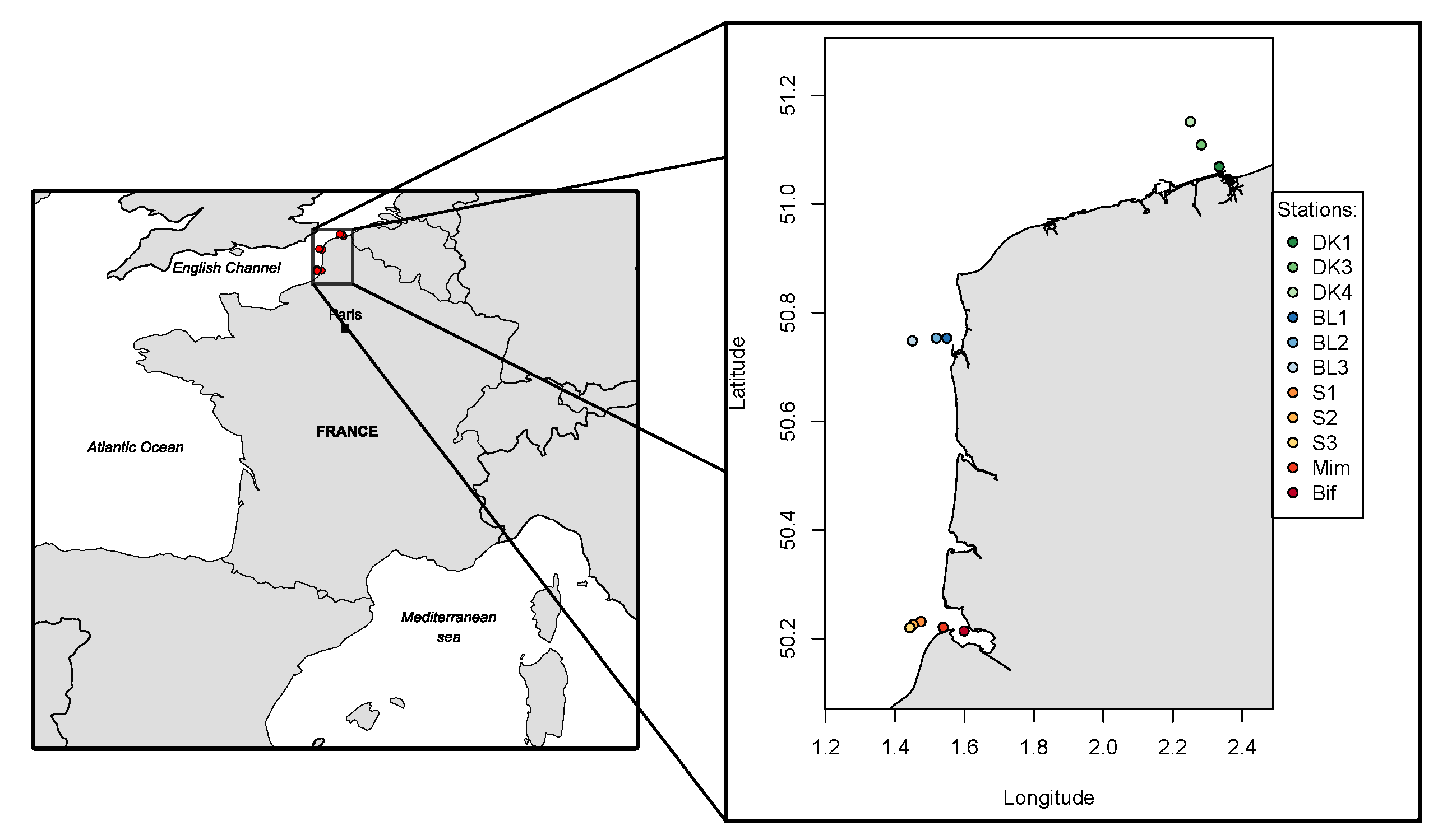
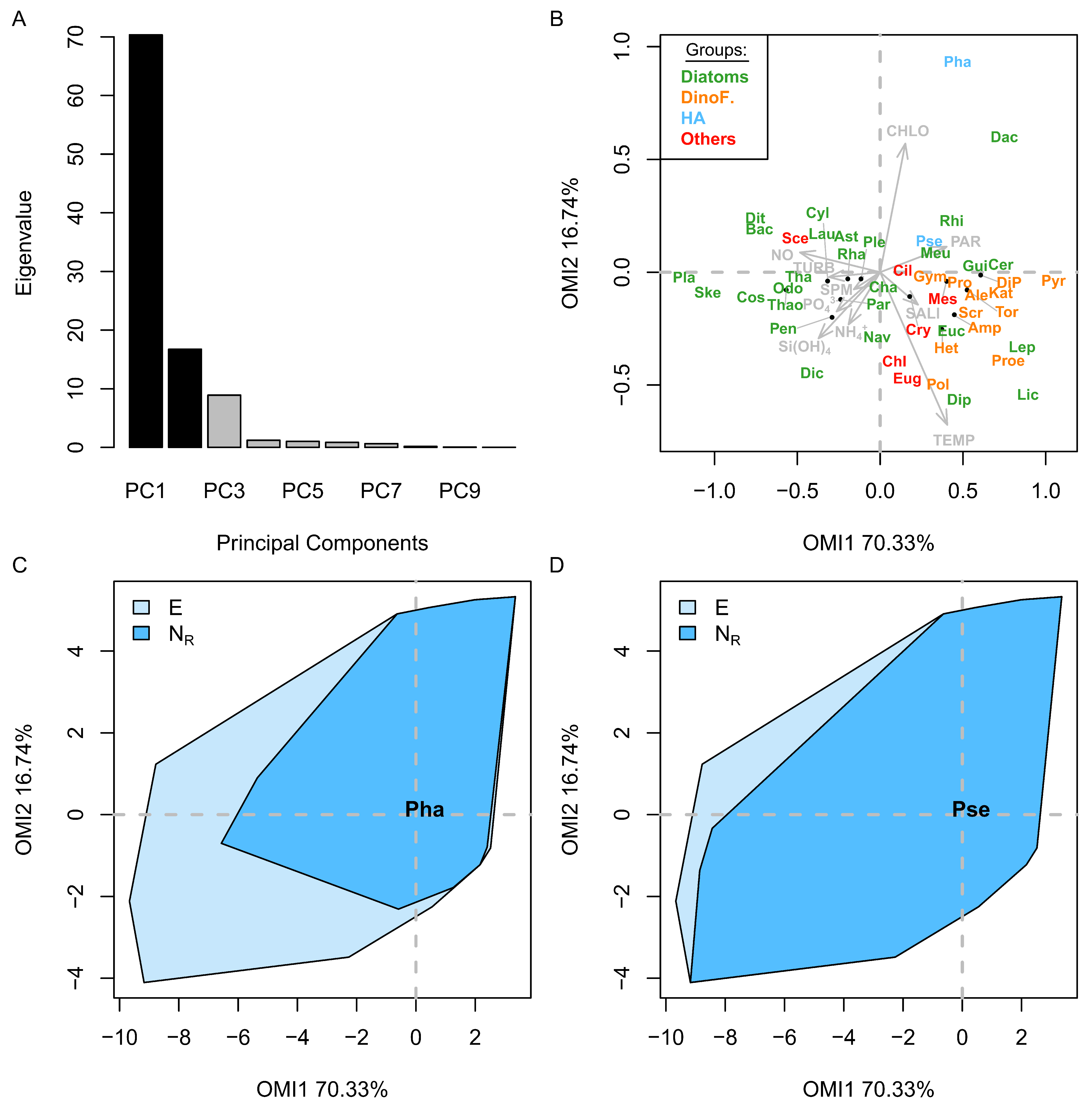
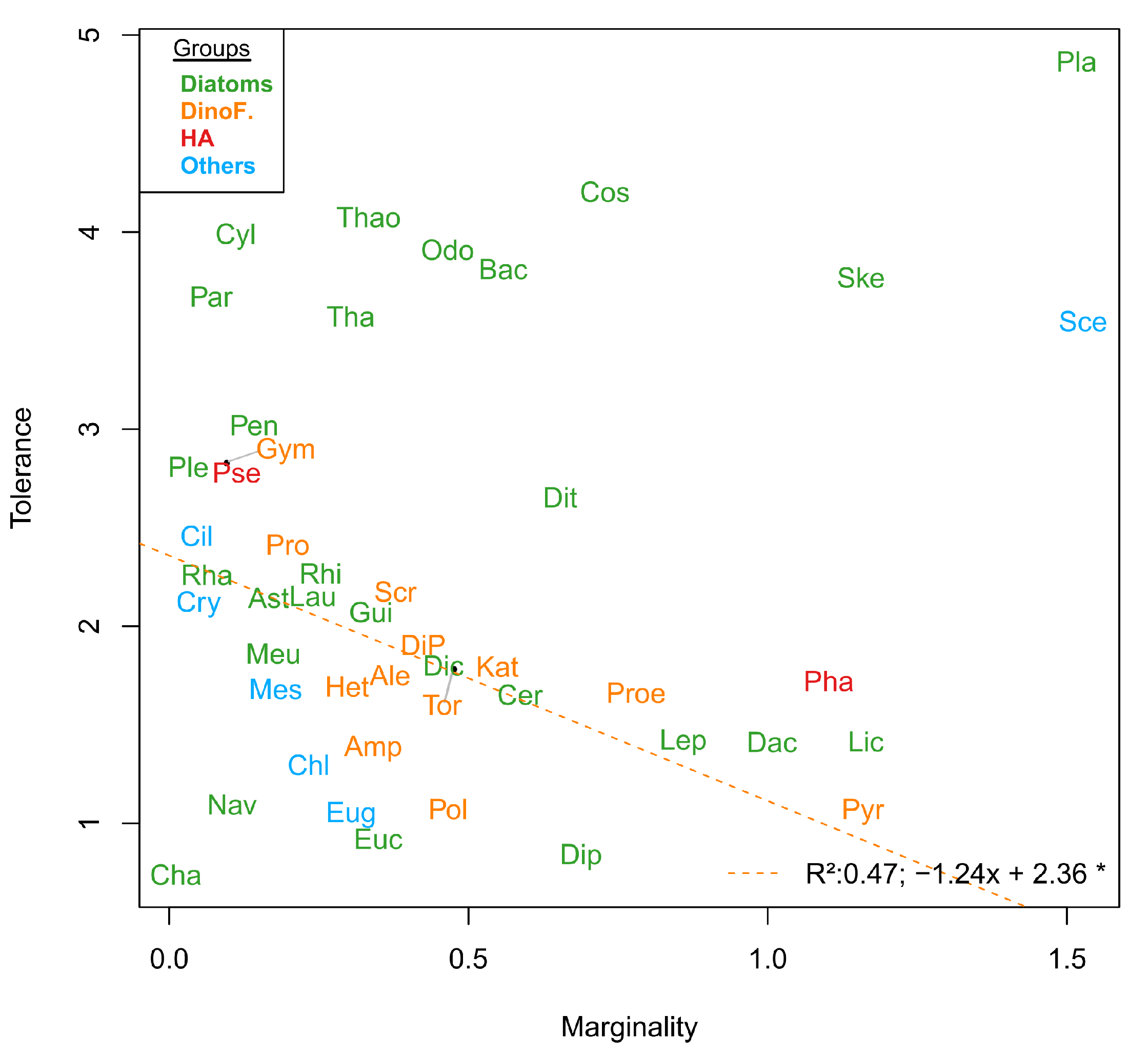
The environmental conditions defined by the space E, within which 47 phytoplankton species niches were calculated by OMI analysis, were divided into two different environment types—estuarine and winter-like conditions, and the more open-water and summer-like conditions (
Figure 4). They were suspected as the REPHY/SRN stations are mostly located in coastal waters (
Figure 1), and their proximity to rivers created a salinity and turbidity gradient between the sampling, which was also found in the PERMANOVA results (
Table 2). The correlation between irradiance and temperature was expected as the eastern English Channel follows the seasonal cycle which is strongly driven by these two environmental factors [
76,
77]. The phytoplankton community was distributed along the gradient created by nutrient concentration and light, reflecting the seasonal cycle (
Figure 4B). The strong seasonal cycle within the environmental parameters was also apparent in the results of PERMANOVA (
Table 2). The segregation between the diatoms (on the left in
Figure 4B) and the dinoflagellates (on the right in
Figure 4B) niche positions is typical of the species seasonal succession [
78]. In the EEC, the dominance shift in the succession from the diatoms to the dinoflagellates is caused by the decline of silicate concentration, which becomes a limiting factor for diatom growth. The dinoflagellates, which do not require silicate, can grow and overcome them [
79,
80]. The two species of interest
Phaeocystis globosa (Pha) and the complex
Pseudo-nitzschia (Pse) spp. preferred summer-like conditions, with Pse having a larger realized niche (N
r) than Pha. Pse appeared to be a much more generalist species, being more tolerant to environmental variation and found all year round (
Figure 6A) compared to Pha (high tolerance and lower marginality, see
Figure 5). Pha has a distinct habitat because it appeared during a time of year when there is high productivity from the community as expressed by the high concentration of chlorophyll-
a (
Figure 4B). Herein, the concentration of chlorophyll-
a was used as a proxy for the net productivity at time
t when the sampling occurs, as the grazing has already happened and is therefore reflected in the sampled value. To understand the relationship, the bloom of Pha needs to be put back in the ecological context. Along the French Coast of the eastern English Channel,
Phaeocystis globosa competes with diatoms, such as
Pseudo-nitzschia spp., for resources, especially nitrogen, phosphate and light, but only when silicate was available [
35]. The “silicate-Phaeocystis hypothesis” [
81,
82] determined the appearance of
Phaeocystis spp. The silicate concentration defined the duration and stability of the diatom community, which in turn determined the
Phaeocystis globosa appearances.
One of the main parts of the study was to create an algorithm with which the blooms of the two species groups of interest,
Phaeocystis globosa (Pha) and the complex
Pseudo-nitzschia spp. (Pse), were detected for each time-series of each sampling station. Even with the first condition of the algorithm, which did not consider as a bloom maxima lower than 10,000 cells·L
, we still managed to detect a significant number of blooms for both taxa. Our expectation was to detect at least one bloom per year per taxa due to the recurrence of the HAB events in these waters [
27,
28,
29,
48], making an expected bloom count of 454. For a total of 363 blooms detected, 80% of our expectations were met, despite some encountered issues. For some time-series (see
Figures S1 and S2 in Supplementary Materials), the estimated smooth spline at the beginning was not adequate for the detection of a bloom during the first years of the time-series. This issue was frequent and could be addressed in the future by imposing a maximum or a minimum starting point value for the estimated smooth spline. The other problem encountered was mostly related to taxonomic data. The algorithm did better at detecting the bloom of Pha, where the spline generated high peaks in a short time span, compared to Pse, which was not as clear. We think this was due to the taxa Pseu, which group several species of
Pseudo-nitzschia spp. instead of mostly one for Pha. The
Pseudo-nitzschia spp. complex from the REPHY/SRN dataset group, in the EEC, at least three species (
P. delicatissima,
P. pungens,
P. fraudulenta) which can only be identified by closer examination of their morphology with a Scanning Electron Microscope (SEM) [
31]. The diversity of unrecognized species in Pse caused an overall constant presence of the taxa and therefore generated large blooms that did not fit the 2nd and/or 3rd condition for them to be considered further. For future use of the algorithm, the taxa studied should avoid species grouping if possible and tweak the algorithm conditions (minimum abundance threshold for bloom, percentage of difference between high and low points, days of extended bloom) for each taxa instead of using the same for all of them.
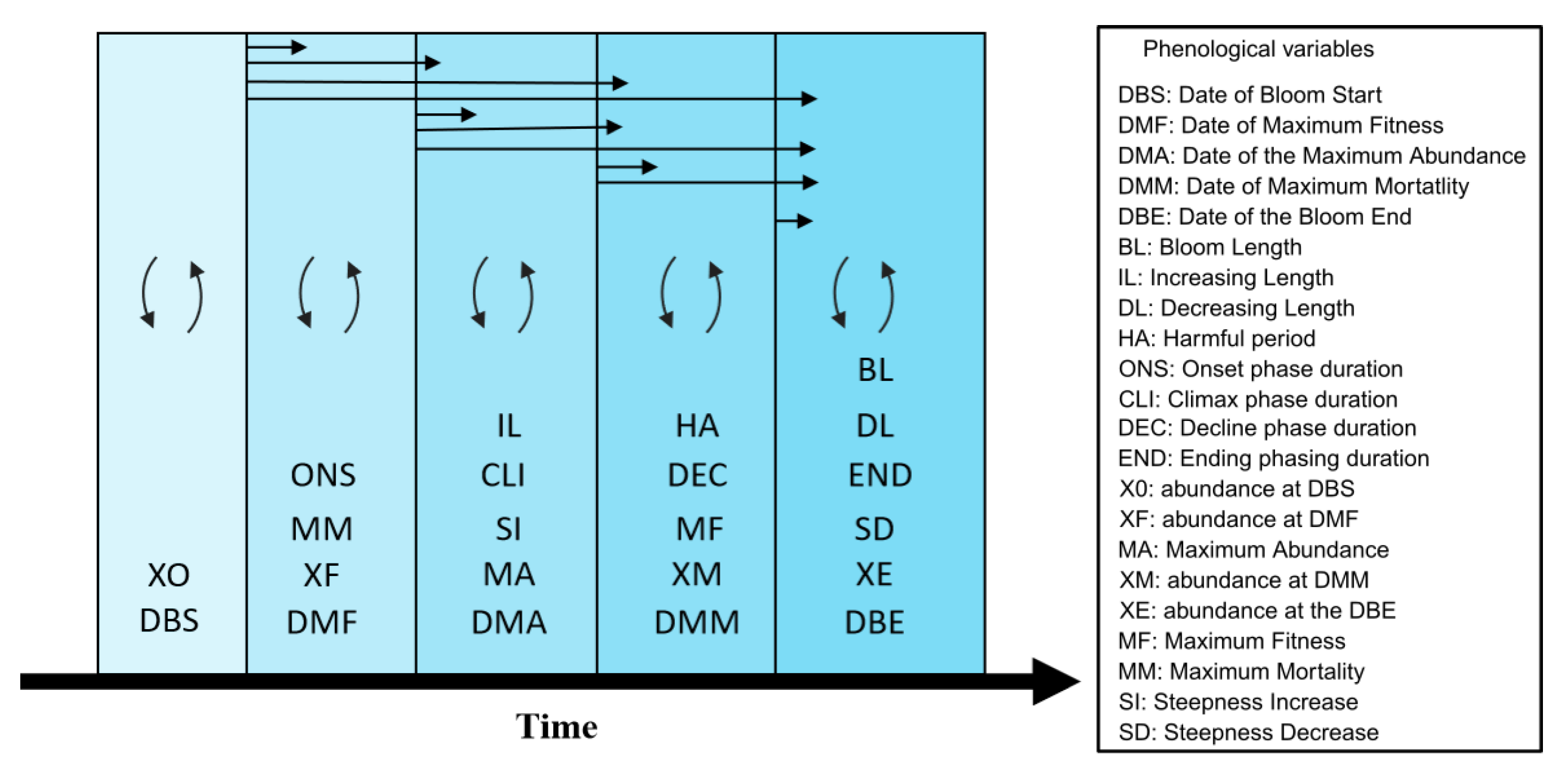
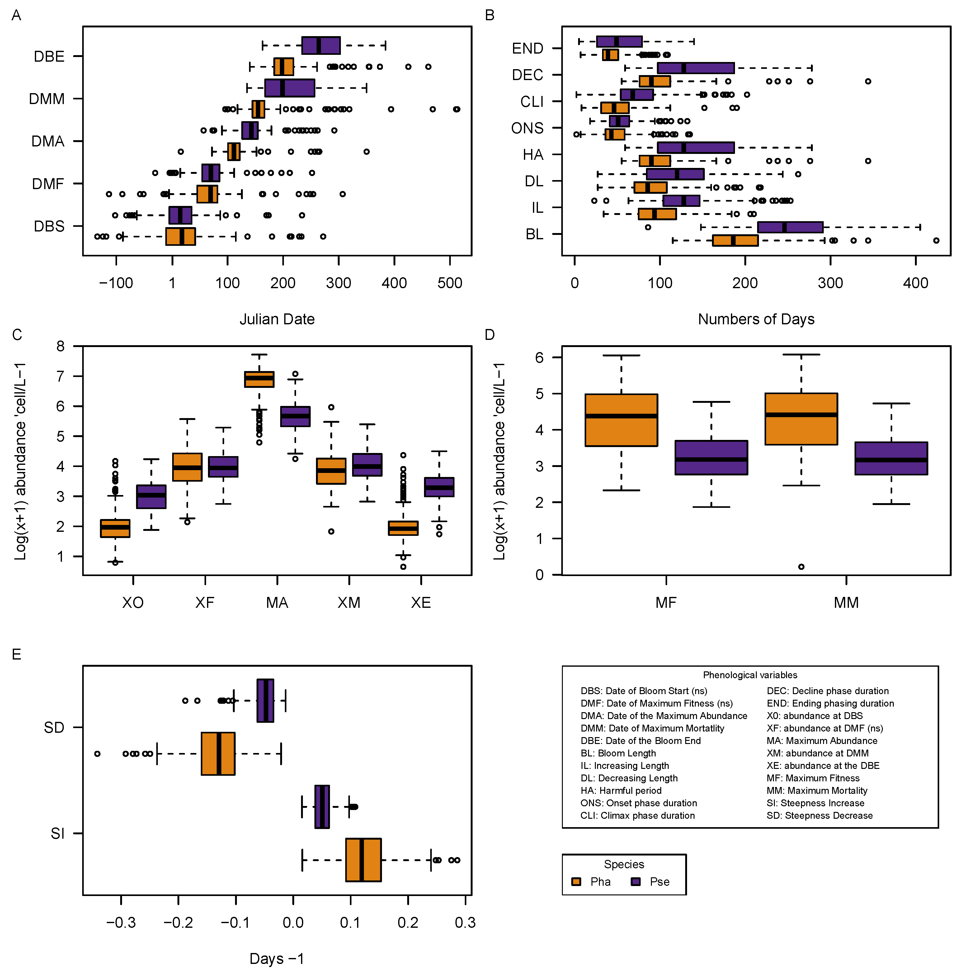
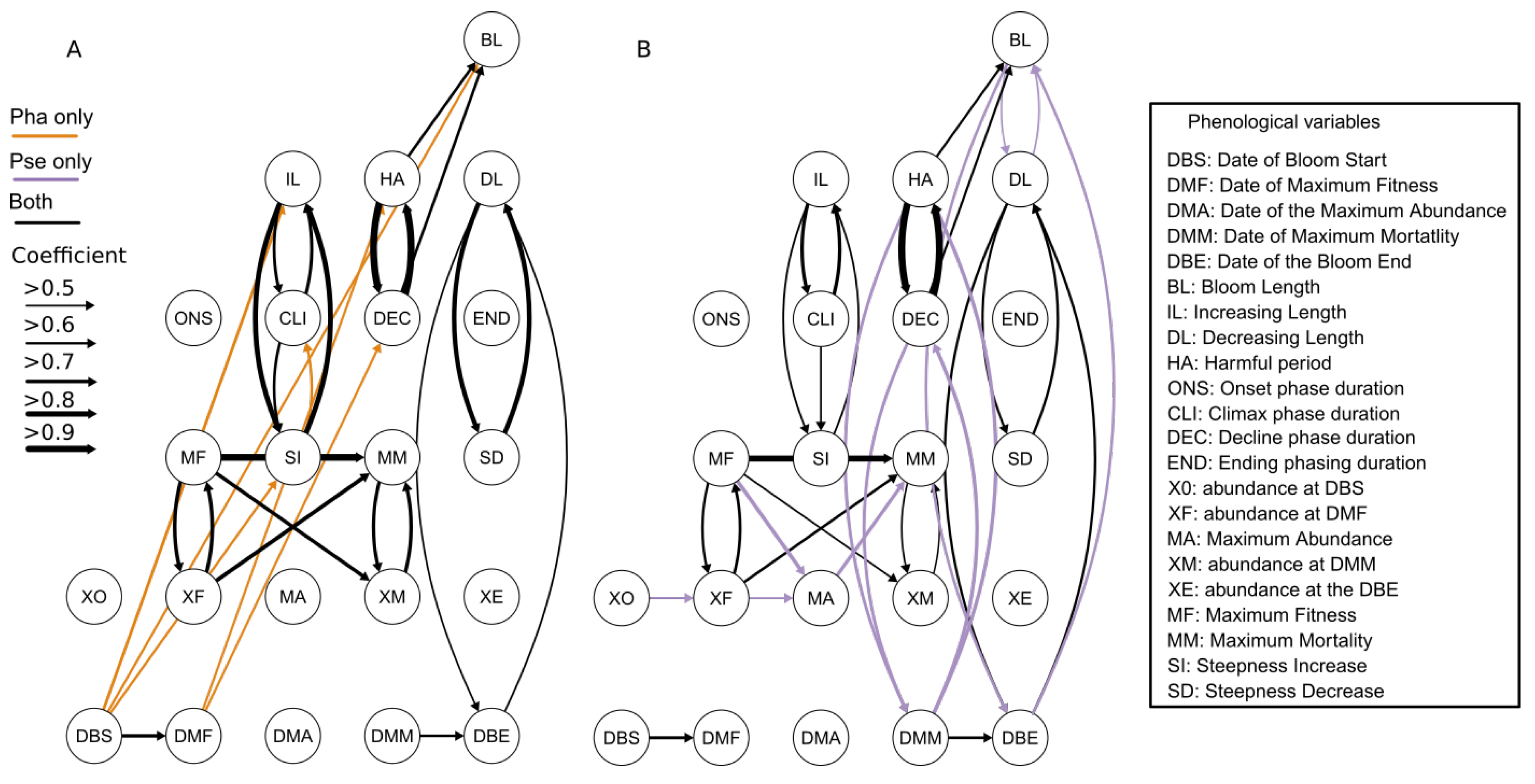
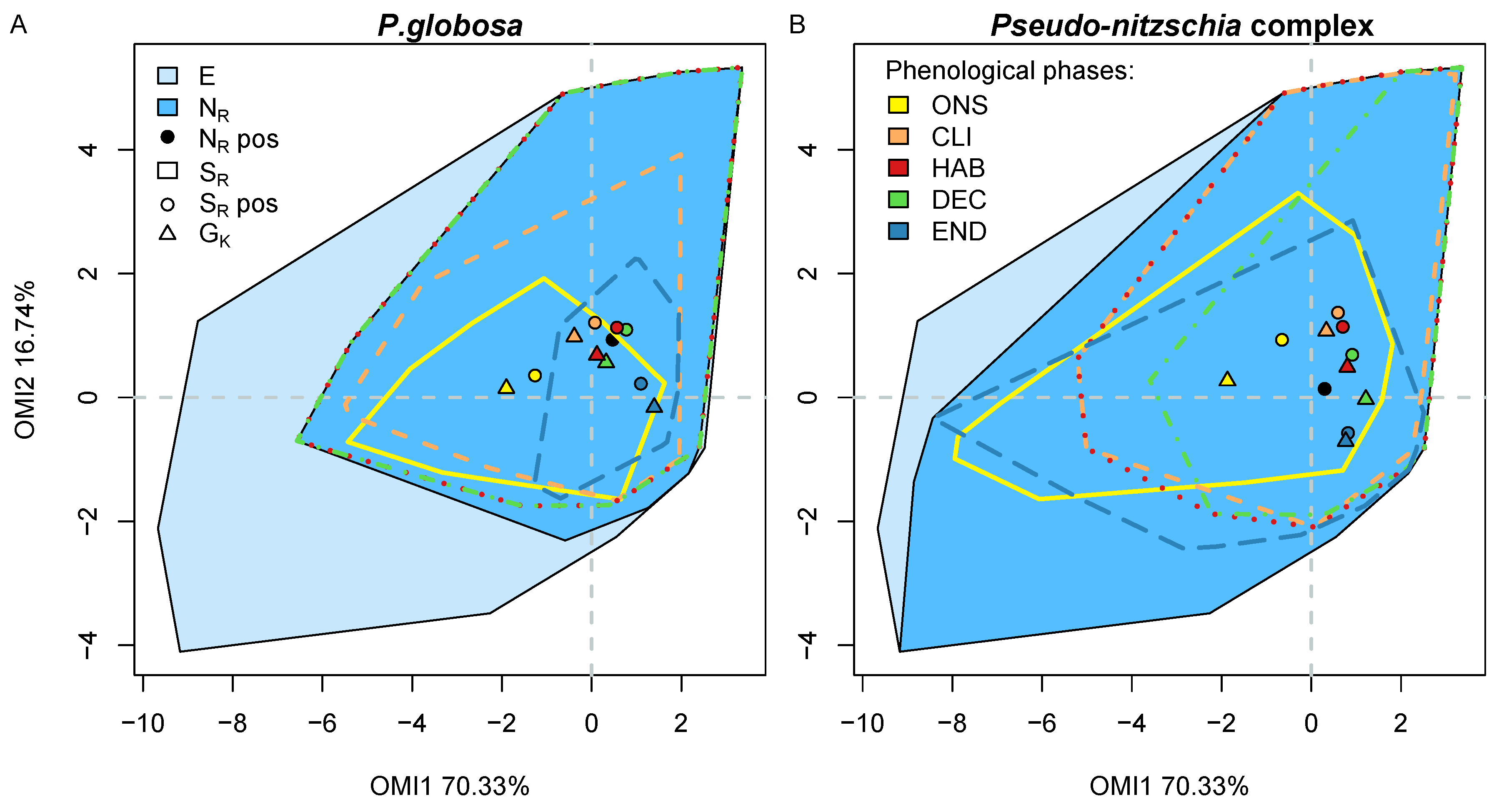
From the bloom detected with the algorithm, a total of 22 phenological variables were extracted from each bloom for the two taxa giving a detailed description and quantification of the bloom characteristics. A Kruskal–Wallis Rank Sum test revealed that for most of the phenological variables, the two taxa Pha and Pse had significantly different blooms (
Figure 6). These results were expected as the two taxa are from two distinct groups of phytoplankton—
Phaeocystis is a marine haptophyte (Lancelot et al., 1994) and the complex
Pseudo-nitzschia is a cacillariophyte [
17]—and would not have the same interaction with the environment or resource requirements. This difference in requirement can be seen in the evolution of the phenological subset K (
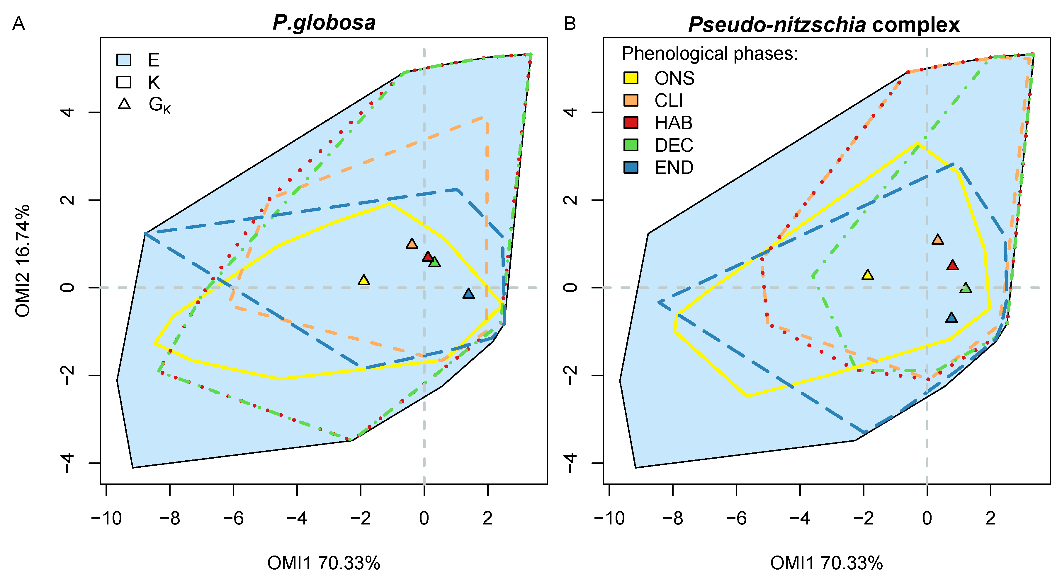
Figure 8). At the beginning, the onset (ONS) subset was relatively similar for the two species (yellow polygon in
Figure 8) but their subniche was quite different (yellow polygon in
Figure 9). Pse had a greater affinity to high concentrations in nutrients, and most likely Si(OH)
4, than Pha and, for similar values of diversity indexes, Pha was more affected by biological interactions than Pse (
Table 6). The high concentration in Si(OH)
4 prevented Pha from realizing its subniche properly due to competition with the diatoms for the other resources. However, Pse was more suited to compete as it was favored by this type of habitat. The high competitiveness community during the ONS phase of the bloom was also supported by high diversity indices, which indicated a relatively even community (J) with a high diversity (H) (
Table 6).
Later, when the concentration of Si(OH)
4 reduced across the climax (CLI), harmful (HAB) and decline (DEC) subsets, this was when Pha actually managed to increase the size of its subniche as the environment changed to favor its growth despite some biological constraints (
Figure 8). Similarly for Pse, this was when the taxa managed to fully occupy its potential subniche (
Table 6). Despite the same number of species, the diversity indices decrease as the remaining taxa in the community were more dominant. A lower phosphate concentration allowed
Phaeocystis globosa to out-compete the diatoms, as
Phaeocystis globosa has the capacity to store phosphates within its colony matrix [
83,
84] coupled with its lower P requirements [
85]. Additionally,
Phaeocystis globosa has a strong competitive ability to obtain nitrogen [
86], along with a lower concentration of silicate, and inhibited the diatom community from blooming. Since the
Pseudo-nitzschia spp. Complex is an assemblage of species, its presence over other taxa can be for multiple reasons. In the waters of the eastern English Channel, the
P. seriata complex is known to be abundant when low DIN and Si(OH)
4 concentrations result in low Si/N ratios [
31]. Furthermore, limitations in silicate have been shown to favor
Pseudo-nitzschia abundance and toxicity [
87,
88].
P. multiseries was able to out-compete other diatom species when silicate concentration was limited compared to nitrogen [
89]. Therefore, in similar environmental conditions, Pha and Pse can out-compete other diatom species of the community. It was also during the CLI, HAB and DEC phases of their respective bloom that the species subniche positions were the closest to the realized niche positions, and therefore the most harmful. Finally, in the END phase, the two taxa were prone to higher biological constraints as the environment changed in favor of higher diversity (
Table 6), reducing the subniche of Pha and Pse. During the END phase of the bloom, Pha and Pse were more subject to biological restrictions (
Table 6). Overall, Pse appeared to be more limited by environmental conditions than restricted by biological interactions. However, Pha was always competing for resources, regardless of whether the environment was limiting or not.
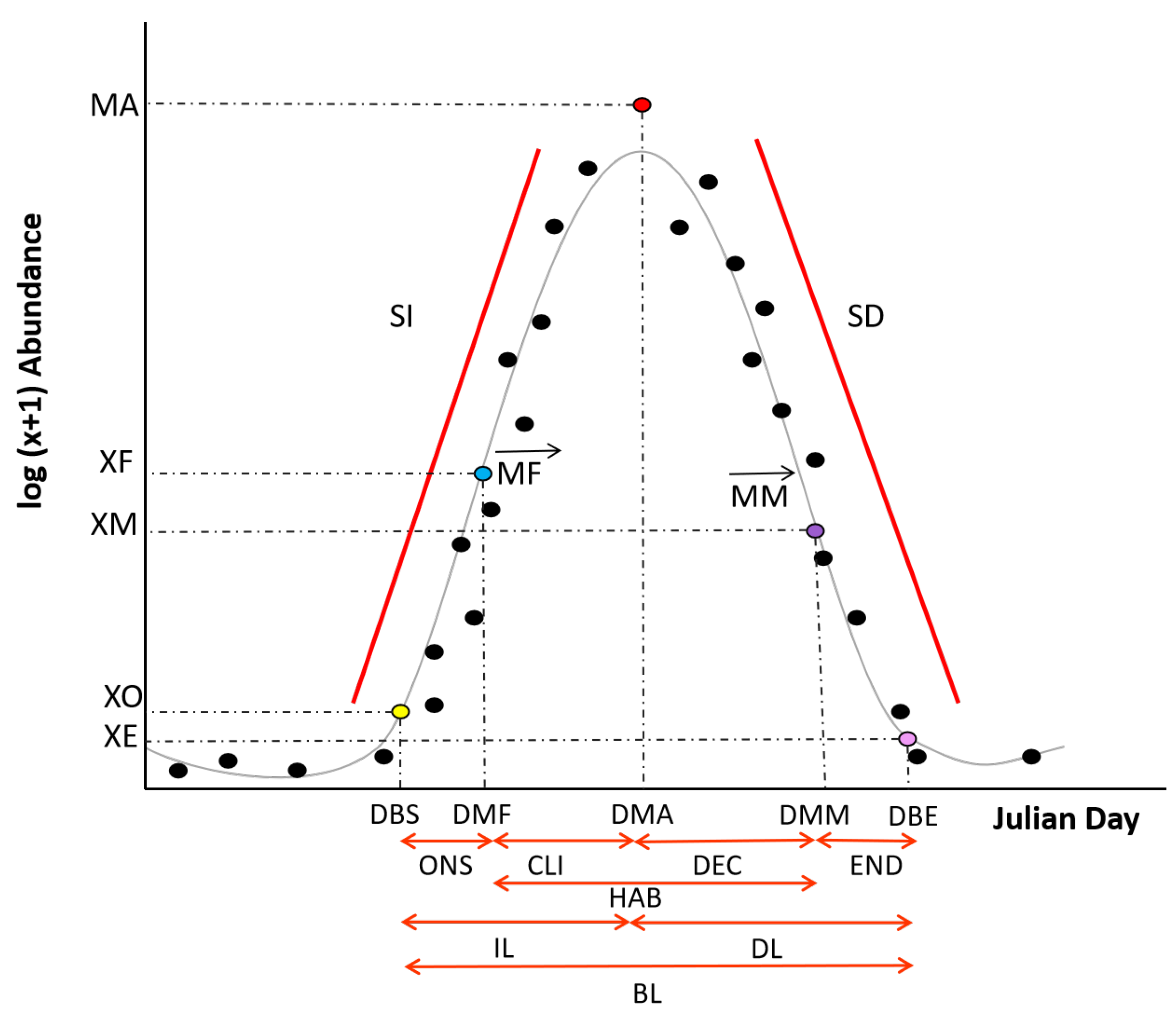
The blooms of the two taxa started at approximately the Date of Bloom Start (DBS) and Date of Maximum Fitness (DMF). Pha had a short but intense burst in abundance expressed by its small Bloom Length (BL), high Steepness Increase (SI) and low Steepness Decrease (SD) with a high Maximum Abundance (MA), while Pse had a more softened (lower SI and higher SD) bloom which lasted longer (longer BL) and at lower abundance (reduced MA) (
Figure 6). For a similar DBS and DMF, the two taxa appeared to have two different phenological characteristics, which had led to different phenological strategies (
Figure 7). For both of them, the DBS and DMF cannot be used to determine the other key dates of the bloom, in particular the Date of the Maximum Abundance (DMA), which could be a useful bloom variable to predict for coastal resource management [
13]. Furthermore, the lack of relationships between dates and abundance variables imply that the processes that are influencing the bloom timing (dates) and intensity (abundance) are different (
Figure 7). Most likely, environmental conditions define the timing, and the biological interactions determine the abundance.
The taxa’s bloom length (BL) appeared to be more related to the length of the HAB and DEC phase of the bloom than to the earlier phases. Moreover, the length of the HAB phase would mostly depend on the length of the DEC than on the CLI phase (
Figure 7). These links suggest that the duration of the bloom would depend on the time it takes for the corresponding taxa to decline after being established in the water column. The bloom of Pha and Pse would therefore be limited in time by external factors, either environmental [
90,
91,
92] or biological [
41,
93,
94]. It has already been reported that the spring bloom ends when the resources become limited or when the population of the grazers become sufficient to reduce the bloom size [
95].
Phaeocystis globosa is well known to change life forms, single cells and colonies in response to grazing [
96]. It responds to different chemical cues released by different predator species and is capable of switching from single cells to colonies when grazed by ciliates [
97,
98]. Inversely, grazing copepods can significantly decrease
Phaeocystis spp. and its colony numbers by 60–90% [
97]. However, what is unknown is the impact these limiting factors have on the duration of the entire bloom from start to end. The increasing length (IL), which consisted of the ONS and CLI duration, would have happened as long as the conditions were right for the taxa to bloom. The bloom would increase indefinitely if it were not for other environmental and/or biological factors to intervene to stop the increasing phase and start the DEC. Therefore, the efficiency of the limiting factor, in this case predation by copepods for Pha, would define the bloom duration of the taxa. The study of the environmental and/or biological factors occurring during the DEC are paramount if one wants to find a potential environmental and/or biological tools to reduce the effect of HAB.
The relationship between Maximum Fitness (MF), abundance at DMF (XF), Maximum Mortality (MM) and abundance at DMM (XM) suggested a symmetry of the blooms. In suitable environmental and biotic conditions, the abundance XF would intimately affect the MF or growth rate of the population and vice versa (
Figure 7). In unsuited environmental and/or biotic conditions, the abundance XM would intimately affect the MM of the population and vice versa. The more abundant the population (XF), the higher the number of individual in the next generation, which would also reproduce and consequently increase the growth rate (MF) (
Figure 7). By contrast, during the decreasing phase of the bloom, the more abundant the population XM, the higher the mortality (MM) in the population as more individuals perish due to unfavorable environments or by lethal interaction with other organisms. During the increasing phase, a positive loop exists between XF and MF whereas during the decreasing phase, a negative loop exists between MM and XM. Furthermore, the initial speed of increase (MF) and abundance (XF) has a direct impact on future mortality rate (MM) of the population (
Figure 7). We explain these correlations to be similar to the process between the XM and MM but with higher temporal lag. The intensity of the positive loop during the increase would eventually affect the MM when the environmental and/or biotic conditions become less suitable to the population later in the year. The balance between the positive and the negative feedback loop during the increasing and decreasing phase of the bloom creates the known inverse U-shape characteristics of the bloom in the time-series.
Despite the common correlation between the phenological variables that the two taxa had, they also had some links that are unique to each of them. For Pha, the DBS has a direct effect on the IL, BL and SI (
Figure 7A). The DBS appeared important for Pha, as not only did it mark the start of bloom, but it would also determine the duration of the bloom with its SI and therefore affecting the duration of the IL. To understand the relationship, it is necessary to put the bloom of Pha back in the ecological context. As previously mentioned, in the eastern English Channel, the appearance of
Phaeocystisspp. was governed by the “silicate-Phaeocystis hypothesis” which competes for nutrient resources with the diatoms [
81,
82]. A previous study showed that the maximum in N:Si corresponded to the start of the
Phaeocystis spp. bloom [
35,
99,
100] giving a short window for the taxa to out-compete the diatoms. The reduced concentration of silicate represents a short environmental opportunity for
Phaeocystis to bloom fast and out-compete the diatoms, which make the DBS a critical phenological variable. Similarly, we suspected the connection between DMF and the two bloom phases HAB and DEC was potentially caused by mismatching (
Figure 7A). As we mentioned previously, the HAB, and more specifically the DEC phase duration, would appear to depend on the efficiency of the limiting factors and/or the biological interactions to reduce the taxa population during its bloom. Therefore, the timing at which Pha reaches its highest fitness potential (DMF) is crucial for taxa life history events (such as bloom) in a seasonal cycle [
101,
102,
103] as it allows it to eventually avoid competition and/or predators [
43]. The timing of life history events (such as the maximum growth or MF) in a seasonal cycle can have an important fitness consequence [
43], in this case the duration of the bloom.
The relationships between the phenological variables were more numerous for Pse and could potentially be used to build a predictive model. From the 22 phenological variables, only three were left unbound to another variable. Moreover, from the 32 significant links, only one was isolated from the rest, which expresses great interconnectivity between all the phenological variables. The bloom of Pse seemed to be characterized by two systems. The first system shaped the abundance of the bloom: from the start (XO) to the maximum mortality (XM) by passing through the bloom balance process (the relationship between MF, XF, MM and XM). The continuous influence of three consecutive abundance variables (XO->XF->MA) could potentially lead to helping to create a statistical tool for predicting the intensity of the bloom maximum (MA), which would be useful for coastal resource management. The second system was defined by the timing of maximum mortality and end of bloom (DMM and DBE), affecting the HAB and DEC phase as well the BL. The independence of the second system from the first suggested that Pse has no control over its decreasing phase of the bloom, which is most likely being caused by an environmental or biological limiting factor.
The relationships between the SD, DL and DBE can be explained by the way the variables are obtained (See Equation (5)). The calculation of SD depends on DL which in turns was obtained with DBE, which in turns creates the dependencies between the three variables. A similar explanation can be provided for the interdependencies between IL and SI (See Equation (4)). These explanations can only be valid because in both cases the abundance at the bloom start (XO) and at the end (XE) were constantly much lower than at the MA, increasing the dependencies between the steepness variables (SI and SD) with the tendency length (IL and DL) (
Figure 6). This was verified by the stronger relationship between IL and SI for Pha than for Pse (
Figure 7). It would not have been the case if XO, XE and MA had much greater variations in their respective values. By construction, the direct relationships between SI, MA, XO and IL and between SD, MA,XE and DL are suspected if XO, XE and MA were not as constant.
In perspective, this kind of study can be repeated on other harmful species found in the different regions, such as France, in
Alexandrium minutum in the Bay of Brest [
104],
Lepidodinium chlorophorum in the Bay of the Vilaine [
105] and also
Ostreopsis ovata in the Meditterean Sea [
106]. Each local area could have a statistical map representing the ecological niche of the phytoplankton community, and tracking the environment changes within the map. For each harmful species found locally, an investigation can be done to understand the impact of the seasonal change upon the phenological phases of bloom to develop biological and statistical indicators that could help coastal resource management to act upon the threat of local HAB. As the spatial scale should remain relatively small (regional size at most), the temporal resolution of the data could be increased. In our study, we used the data collected by the REPHY/SRN monitoring network [
49,
50] that is collected once or twice a month. Samples collected at fixed stations are often collected bi-weekly, weekly, or even daily in some monitoring programs, which exposes the detailed changes in phytoplankton variability [
2]. The temporal resolution of the data is paramount for phenological analysis. Phenological studies would gain in detail with a higher frequency data, as more information would give a more precise characterization of the bloom along with the environmental variables. The phenological signal can be better predicted when observed at a fixed station. It will be necessary to identify the year-to-year variability of the source region for the population of interest [
43]. Spatially explicit Lagrangian tracking could be used to provide detailed information on the time and space scales of processes relating to the observed phenology signals. A simple passive particle backtracking shows the variability of advection pathways and source regions (e.g., [
107]). To better disentangle the contribution of advection and population dynamics, backtracking for both physical and biological processes will be helpful [
108,
109].


