Abstract
In this paper, we propose a novel method to enhance the accuracy of a real-time ocean forecasting system. The proposed system consists of a real-time restoration system of satellite ocean temperature based on a deep generative inpainting network (GIN) and assimilation of satellite data with the initial fields of the numerical ocean model. The deep learning real-time ocean forecasting system is as fast as conventional forecasting systems, while also showing enhanced performance. Our results showed that the difference in temperature between in situ observation and actual forecasting results was improved by about 0.5 °C in daily average values in the open sea, which suggests that cutting back the temporal gaps between data assimilation and forecasting enhances the accuracy of the forecasting system in the open ocean. The proposed approach can provide more accurate forecasts with an efficient operation time.
1. Introduction
In the past 20 years, ocean forecasting systems using data assimilation have been widely used to predict the physical phenomena of the ocean [1,2,3,4]. Most operational ocean forecasting systems assimilate satellite data [2,5,6,7,8]. Satellite data are the most widely used for data assimilation. Sea surface temperature (SST) data play a crucial role in atmospheric, ocean-ice, and coupled systems. Satellite SST data are normally assimilated along with the in situ SST data [9,10].
Synthesized satellite SST data are the accumulation of various satellite data and assimilate in situ observations. Since in situ observation data used for synthesized satellite SST often contain incorrect or missing information, the data are distributed for use after performing quality assurance (QA) and quality control (QC) following a set procedure. During this process, an expert manually performs a manual QC or visual inspection [11,12,13]. Recently, a more efficient method was suggested [14], but has not been widely used yet. Moreover, the synthetic process also takes some computational time [15].
The National Institute of Fisheries Science (NIFS) distributes multi-satellite sea surface temperature data of 1km around the Korean Peninsula by receiving Advanced Very High Resolution Radiometer (AVHRR) satellite data from the National Oceanic and Atmospheric Administration (NOAA). Satellite data from AVHRR equipped with an infrared sensor are distributed approximately two days later after going through the process of assimilating the data of ocean areas that were undetected due to cloud pollution with in situ data or climatology data [16]. Because of this QA/QC process, data from 1–2 days ago are generally used when assimilating satellite data into the operational ocean forecasting system. Therefore, the forecasting simulations do not carry out real-time data assimilation, but hindcast from several days ago [2,17,18,19].
Artificial neural networks, a statistical prediction technique, have been improved with deep learning [20], allowing them to perform highly complex calculations. Therefore, artificial neural networks are now being used to predict various ocean variables, such as water temperature, salinity, ocean currents, etc. [21,22,23,24,25,26,27]. Moreover, various satellite imageries are used for analysis and prediction using deep learning technology [28,29,30,31,32].
Kang et al. [33] proposed a deep-generative-inpainting-network (GIN)-based reconstruction method for sea surface temperature data, and they were able to obtain seamless satellite sea surface temperature data instantly using a deep-learning-based resilience approach. They successfully reconstructed the detailed missing patterns in the cloud regions in infrared satellite sea surface temperature data.
In this study, we reproduced a near-real-time satellite sea surface temperature with the GIN and assimilated with the initial fields of the numerical coastal ocean model in Gyeonggi Bay. Results from the new approach eliminate temporal gaps between the data assimilation and forecasting stage. The proposed system was compared with a control run of the conventional operation, which had a two-day temporal gap.
2. Data and Methods
2.1. Data Assimilation Scheme
Most data assimilation schemes for ocean data can be formulated as:
where is the assimilated field, is the background field, K is the weight, Y is the observations, and H is the conversion matrix, respectively.
In this study, we adopted optimal interpolation, and K is defined as:
where B is the forecast error covariance matrix, which is proportional to the distance between grid positions, and R is the observational covariance matrix, respectively. In order to apply this assimilation scheme, this study used the extracted data in the model and restored satellite SST data. As the specific parameter, the extraction step was set to 5 intervals to make each spatial resolution equal to 25 km, which buffered the diameter of the horizontal direction set to 50 km. Then, the data assimilation scheme was applied according to the Gaussian distribution after setting the error ratio between the model and satellite data as 2-to-1.
2.2. Experiment Method
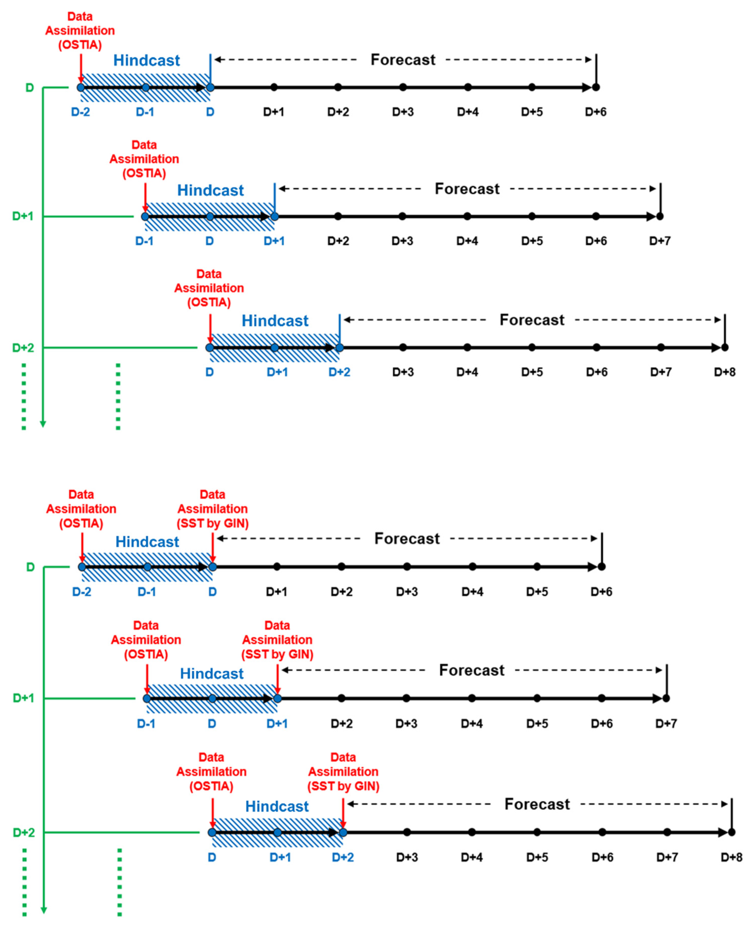
In this study, the SST produced by using a GIN-based reconstruction method for satellite sea surface temperature (GIN-SST) data was assimilated into the ocean model, then we examined the performance of the forecasting system. The forecasting system was built based on the region ocean modeling system (ROMS), a primitive equation, hydrostatic, finite-difference, free-surface model with the general kernel described by Schchepetkin and McWilliams [34]. The performance of the forecasting system was examined with (WGIN) and without (CTRL) the application of an initial field assimilated with the SST produced from the GIN-SST set as the initial date. Following the currently used settings of operational ocean forecasting systems [2,18], CTRL was designed to assimilate satellite SST into the previous state and had a temporal lag of 2 days from the present state (D-2), whereas WGIN assimilated the reconstructed data (GIN-SST) for D-1 and D (Figure 1).

Figure 1.
The timeline of the forecasting systems. The (top) is the control run (CTRL), and the (bottom) is the GIN case (WGIN), respectively.
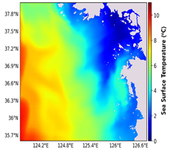
The OSTIA system uses data from a combination of infrared and microwave satellites, as well as in situ data [10]. OSTIA data products are currently the most widely used operational sea surface temperature and sea ice analysis data produced by the Met Office. The OSTIA SST field is produced daily with a resolution of approximately 5 km for the entire region, and it is assimilated by optimal interpolation using 7 types of satellite data (AATSR, AMSR-E, AVHRR-LAC, AVHRR-GAC, SSM/I, SEVIRI, TMI) and sea surface temperature data obtained from buoys and in situ observations (Figure 2).
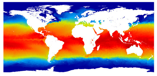
Figure 2.
OSTIA SST data (www.metoffice.gov.uk, assessed on 24 November 2021).
The water temperature data from the Korea Meteorological Administration’s ocean observation buoys in three locations (Incheon, Deokjeokdo, Oeyeongdo) were used for comparison to verify the performance of the experiment. February, May, August, and November, which are the four seasons of the sea, were set as the comparative experiment period.
2.3. Gyeonggi Bay Numerical Ocean Model
The Gyeonggi Bay model was constructed using the ROMS to generate a sigma vertical grid suitable for the strong tides and shallow depth of the West Sea. The dimension of the model was 534 × 545 in longitude and latitude, respectively. The horizontal grid with a 500 m resolution was generated with 15 vertical layers. The domain and bathymetry of the model is shown in Figure 3.
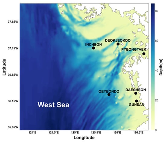
Figure 3.
Model domain and bathymetry (Gyeonggi Bay). Dots indicate buoys’ locations.
Lateral boundary input data, such as sea surface height (SSH), temperature, salinity, and velocities, were generated by interpolating the 1/12°-resolution global ocean forecasting data provided by Copernicus Marine Service. The 0.25°-resolution prediction model data produced by the National Centers for Environmental Prediction (NCEP) Global Forecast System (GFS) were interpolated according to the domain of the West Sea model to produce the meteorological boundary data. TPXO (OTPS) provided by Oregon State University was used for tides. TPXO8.0 is the most accurate global ocean tidal model, which provides TOPEX/Poseidon and Jason satellite data, as well as OTIS data [35]. In this study, we adopted 8 tidal components (M2, S2, N2, K2, K1, O1, P1, and Q1).
There is a difference between the two initial fields (WGIN and CTRL). For CTRL, an initial field produced by assimilating OSTIA SST data using the optimal interpolation (OI) at the time of forecast d-2 was used. For WGIN, an initial field produced by assimilating the GIN-SST data from d-day, the starting point of the forecast, and the background (model result) from CTRL using OI were used as the input data. Table 1 shows a comparison of CTRL and WGIN.

Table 1.
Comparison of the configuration of the two systems, CTRL and WGIN.
2.4. GIN-SST (Instantly Reconstructed SST Field Using GIN)
The undetected areas in the satellite SST fields are instantly restored by the GIN method [33]. The GIN uses random masks to generate artificial missing regions, and the adversarial networks, which consist of a generator and a discriminator, were optimized by loss function values between the original and generated data. The size of the random masks was randomly generated rectangles whose size was randomly determined in the range from 32 px × 32 px to 256 px × 256 px.
The restored SST fields were near-real-time and assimilated into the initial fields of the ocean numerical model. The satellite images are provided at 1 km resolution by the NIFS, which are the synthesis of AVHRR, in situ observations, and climatology. The structure and learning process of the GIN model is shown in Figure 4, and the data including the missing data due to clouds (Level 2) were used as the input image to the GIN-SST model. The learning was carried out in two stages to enhance the accuracy, which consisted of rough learning and fine-tuning.
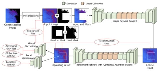
Figure 4.
Structure of the GIN-based reconstruction method for satellite sea surface temperature data.
3. Result
In this study, we used ocean temperature data provided by Korea Meteorological Administration’s (KMA) ocean observation buoys located at Incheon, Deokjeokdo, Oeyeongdo, and the Korea Hydrographic and Oceanographic Agency’s (KHOA) ocean observation buoys located at Pyeongtaek Dangjin Port, Daecheon Beach, and Gunsan Port for verification. The locations of the buoys are shown in Figure 3. Numerical forecasting results from CTRL and WGIN were compared with observations.
3.1. GIN-SST
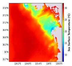
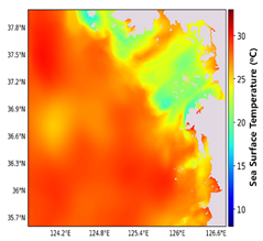
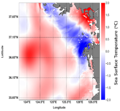
In order to conduct the experiments for February, May, August, and November of 2018, the missing data were reconstructed from the NOAA Level 2 SST data for each month. Figure 5 is the result (output data) produced by the GIN-SST model from the Level 2 SST images (input data) of the 13th of each month. The result was used as the observation data for data assimilation in the WGIN. Since the 2D image data generated through the GIN-SST model are represented in RGB color, we converted the RGB color into ocean temperatures (Figure 6). SST produced via the GIN showed RMSE differences ranging from 0.8 to 2.05 compared to OSTIA (Figure 5). To examine the performance for each season, the monthly average of the RMSE for February, May, August, and November are provided in Figure 5. The results showed the highest RMSE in August and the lowest in February, respectively.
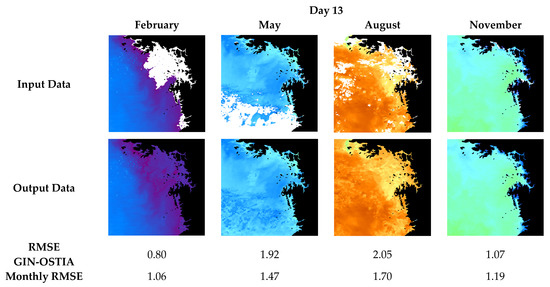
Figure 5.
Reconstructed SST data by the GIN.
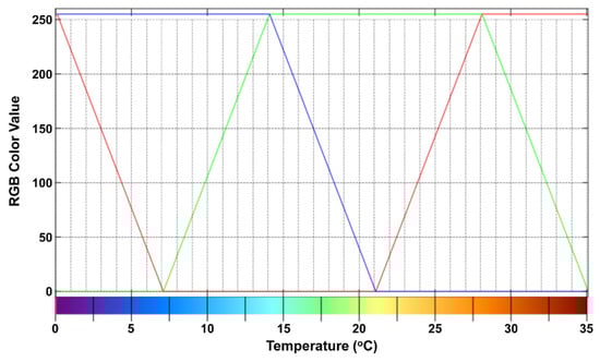
Figure 6.
Matching graph that maps the RGB color values to the corresponding temperature values to convert the original ocean satellite image into the temperature value matrix.
Comparing the GIN production results and OSTIA SST for each buoy observation, the RMSE for the entire period for observation buoys located off the Gyeonggi coast (Deokjeokdo, Incheon, Oeyeongdo) was 0.34 in the GIN, which was slightly less than OSTIA (0.4), and the coastal observation buoys (Pyeongtaek, Daecheon, Gunsan Port) showed a large difference with 0.82 in the GIN and 0.44 in OSTIA (Table 2). The considerable difference in the RMSE between the coastal and open sea region was due to the amount of cloud in the NOAA SST Level 2 input images. In the West Sea coastal area, sea fog or clouds are frequently formed, and consequently, satellite-mounted infrared sensors are not able to detect the SST. Overall, compared to OSTIA, the GIN method showed better performance in the open sea, but the error in the coast was 0.38 higher than that of OSTIA.
Table 2.
Comparison of the GIN and OSTIA with buoy observations.
3.2. Result of CTRL and WGIN
3.2.1. Sea Surface Temperature
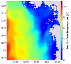
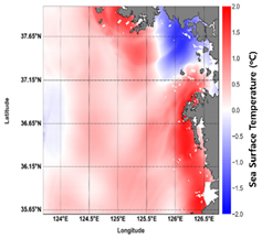
We compared the CTRL and WGIN in February and August, which showed the smallest monthly average errors between the GIN-SST and OSTIA (Table 3). The results from February showed different characteristics between the near-coast region and the open sea. The WGIN showed lower surface temperatures than CTRL overall; however, due to the positive bias of the reconstructed area around the estuary of the Han River (February in Figure 5), the WGIN showed significantly high temperatures in the estuary of the Han River.
Table 3.
Comparison of surface temperature distribution of the WGIN and CTRL.
The results from August, as the results from February, showed CTRL with a higher surface temperature distribution in the entire region compared to the WGIN. However, CTRL simulated a lower surface temperature distribution in the boundary region between the coast and the open sea.
3.2.2. Comparison between Forecasts and Buoy Observations
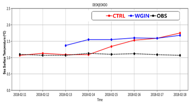
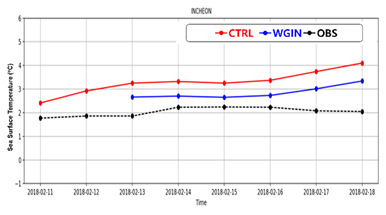
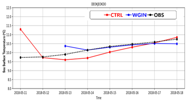
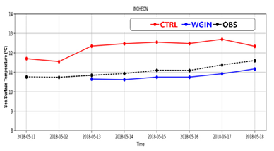
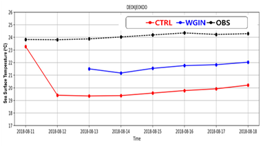
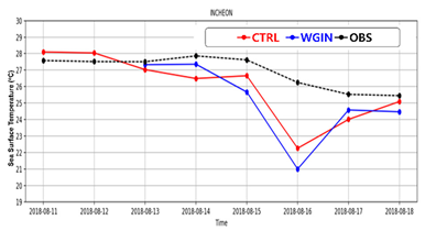
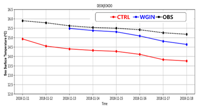
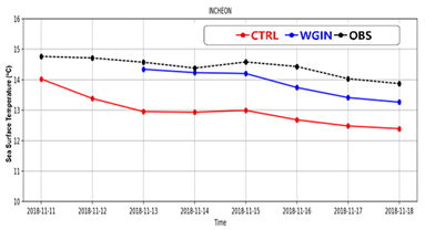
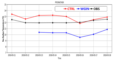
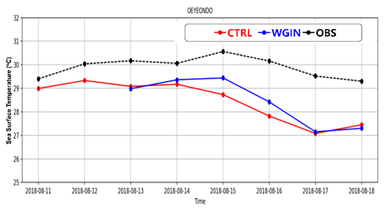
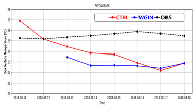
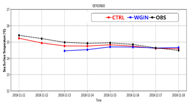
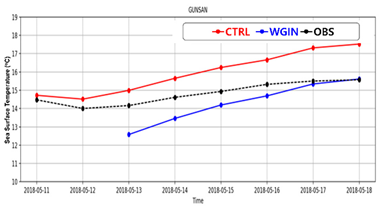
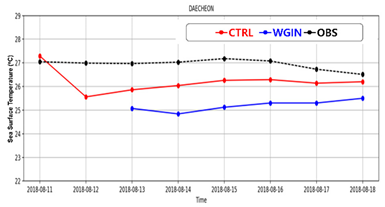
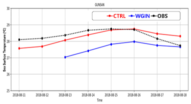
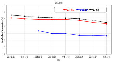
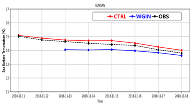
The prediction accuracy of CTRL and the WGIN in the Gyeonggi bay forecasting were compared with buoy observations in times series of daily mean ocean temperature (Table 4, Table 5 and Table 6). The time series represents the six-day temperature prediction from the 13th to the 18th of each month. The red line represents CTRL, the blue line the WGIN, and the black line the observation data, respectively.
Table 4.
Time series comparison of CTRL (red), the WGIN (blue), and observations (black) at the Deokjeokdo (left) and Incheon (right) buoy stations, respectively. The top, second from the top, second from the bottom, and bottom figures indicate February, May, August and November, respectively.
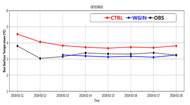
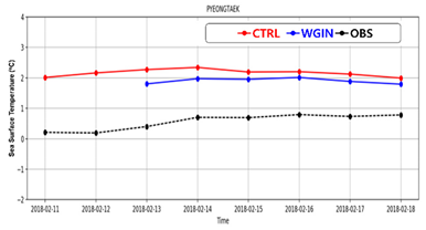
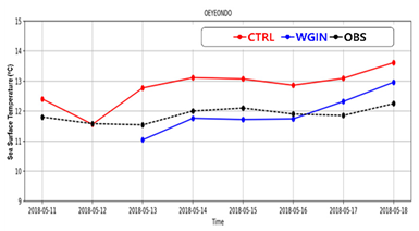
Table 5.
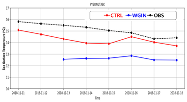
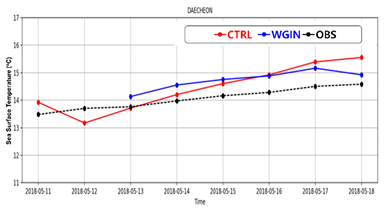
Same as Table 4, except for Oeyeondo (left) and Pyeongtaek (right).
Table 6.
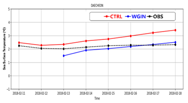
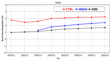
Same as Table 4, except for Daecheon (left) and Gunsan Port (right).
The results of February showed higher bias errors in CTRL, while the WGIN showed better results at five points, except for Deokjeokdo. However, in the results from May, August, and November, the WGIN showed better performances in the open ocean area (Deokjeokdo, Incheon, Oeyeondo), whereas CTRL showed better results in the coastal area (Daecheon, Gunsan, Pyeongtaek).
The higher errors of the WGIN in the coastal areas were correlated with the higher errors of the GIN-SST results in May, August, and November.
Table 7 represents the RMSE with buoy observations of CTRL and the WGIN. Open ocean and coastal area are distinguished by the distance (10 km) from the coast. At the observational sites in the open ocean, the WGIN showed a lower RMSE (1.10) than CTRL (1.68), whereas in the coastal areas, CTRL (1.15) was better than the WGIN (1.44).
Table 7.
RMSE with buoy observations of CTRL and the WGIN.
4. Summary and Discussion
In this study, we developed a real-time operational ocean forecasting system using the assimilation of satellite data restored instantly using the GIN. The conventional operation of data assimilation has a temporal delay of several days, due to the complex reconstruction process of satellite data. The proposed system reduced the temporal gaps between the start of prediction and assimilation.
The data assimilation process attempted to minimize the initial condition errors by incorporating observations into the model data. However, due to the delayed provision of observations due to the QA/QC procedure, a forecast would start several days prior to the present state. Therefore, errors increased during the temporal gaps between the data assimilation and the start of forecasting.
The GIN method had structural errors. Firstly, the satellite imagery had noises around the coastal area due to land. Secondly, when the ratio of the missing region was high, the GIN depended on climatological monthly average values and generated more errors. Due to these problems, the WGIN showed enhanced surface temperatures in the open ocean area, whereas CTRL was better in the coastal area.
Recently, deep learning has been widely used for oceanic data analysis. We used the GIN for the reconstruction of satellite images and instantly restored undetected areas due to clouds. Time-series-based deep learning prediction [36] is widely used for marine forecasting. Moreover, spatio-temporal prediction is also available using a deep learning method [37]. Consequently, various prediction data can be assimilated into the numerical forecasting system to enhance the accuracy of the forecasts.
The constraint of assimilated observation was determined by the covariance matrix of observations, which were given by instrumental errors. However, the reconstructed data by the GIN contained additional errors during the generator network process. More investigations are required to clarify the error levels due to the GIN and the covariances of the reconstructed data.
The circulation of Gyeonggi Bay consists of complex processes, such as freshwater discharge from the Han River, strong tidal mixing, etc. More accurate data assimilation methods using realistic background error covariance are necessary for advanced research to reduce the initial condition problems [38].
Finally, since the deep learning method is a linear algebraic approach that carries out a massive number of simple instructions, general-purpose computing on graphics processing units (GPGPU) is widely used for calculation. The critical problem of the GPGPU is the amount of memory, which is 24 GB at most. Consequently, the size of the images is restricted to around 256 × 256. Due to such limitations of the GPGPU, the proposed system can only be applied to bay-scale areas only. However, with the recent development of a system-on-chip (SoC) that integrates a CPU and GPU, the size of the memory available for deep learning operations is expected to expand to hundreds of giga-bytes. Therefore, the utilization of deep learning for large scale array data such as numerical model data and satellite images will increase in the future, and the proposed method can be applied not only for bay-scale forecasting, but also used for wide-area simulation.
Author Contributions
Conceptualization, Y.C., Y.P. and J.H.; methodology, Y.P.; formal analysis, Y.P. and K.J.; investigation, Y.C. and Y.P.; writing—original draft preparation, Y.C., Y.P. and J.H.; writing—review and editing, E.K.; visualization, Y.P. and Y.C.; supervision, Y.C.; funding acquisition, J.H. All authors have read and agreed to the published version of the manuscript.
Funding
This research was funded as a part of the project by the National Institute of Fisheries Science (NIFS) of the Republic of Korea (Grant Number: R2021070).
Institutional Review Board Statement
Not applicable.
Informed Consent Statement
Not applicable.
Data Availability Statement
In this paper, the ocean buoy observation data were provided by “Korea Meteorological Administration (KMA)” and “Korea Hydrographic and Oceanographic Agency (KHOA)”. The TPXO data was provided by the “Oregon State University” which is the most accurate tide model result. The NCEP, OSTIA, and SST satellite data were provided by the “U.S. National Oceanic and Atmospheric Administration (NOAA)” and “National Institute of Fisheries Science (NIFS) of the Republic of Korea”. Thanks for providing the data.
Acknowledgments
This research was performed as a part of the project by the National Institute of Fisheries Science (NIFS) of the Republic of Korea. The authors would like to thank for all supports to complete this paper.
Conflicts of Interest
The authors declare no conflict of interest.
References
- Evensen, G. Sequential data assimilation with a nonlinear quasi-geostrophic model using Monte Carlo methods to forecast error statistics. J. Geophys. Res. Ocean 1994, 99, 10143–10162. [Google Scholar] [CrossRef]
- Park, K.S.; Heo, K.Y.; Jun, K.; Kwon, J.I.; Kim, J.; Choi, J.Y.; Cho, K.H.; Choi, B.J.; Seo, S.N.; Kim, Y.H. Development of the operational oceanographic system of Korea. Ocean Sci. J. 2015, 50, 353–369. [Google Scholar] [CrossRef]
- MacLachlan, C.; Arribas, A.; Peterson, K.A.; Maidens, A.; Fereday, D.; Scaife, A.A.; Gordon, M.; Vellinga, M.; Williams, A.; Corner, R.E. Global Seasonal forecast system version 5 (GloSea5): A high-resolution seasonal forecast system. Q. J. R. Meteorol. Soc. 2015, 141, 1072–1084. [Google Scholar] [CrossRef]
- Sotillo, M.G.; Mourre, B.; Mestres, M.; Lorente, P.; Aznar, R.; Garcia-Leon, M.; Liste, M.; Santana, A.; Espino, M.; Álvarez, E. Evaluation of the operational CMEMS and coastal downstream ocean forecasting services during the storm Gloria (January 2020). Front. Mar. Sci. 2021, 8, 300. [Google Scholar] [CrossRef]
- Lee, J.H.; Moon, J.H.; Choi, Y. Comparison of Data Assimilation Methods in a Regional Ocean Circulation Model for the Yellow and East China Seas. Ocean Polar Res. 2020, 42, 179–194. [Google Scholar]
- Margvelashvili, N.; Andrewartha, J.; Herzfeld, M.; Robson, B.J.; Brando, V.E. Satellite data assimilation and estimation of a 3D coastal sediment transport model using error-subspace emulators. Environ. Model. Softw. 2013, 40, 191–201. [Google Scholar] [CrossRef]
- Yang, J.; Ding, S.; Dong, P.; Bi, L.; Yi, B. Advanced radiative transfer modeling system developed for satellite data assimilation and remote sensing applications. J. Quant. Spectrosc. Radiat. Transf. 2020, 251, 107043. [Google Scholar] [CrossRef]
- Waters, J.; Lea, D.J.; Martin, M.J.; Mirouze, I.; Weaver, A.; While, J. Implementing a variational data assimilation system in an operational 1/4 degree global ocean model. Q. J. R. Meteorol. Soc. 2015, 141, 333–349. [Google Scholar] [CrossRef]
- Stark, J.D.; Donlon, C.J.; Martin, M.J.; McCulloch, M.E. OSTIA: An operational, high resolution, real time, global sea surface temperature analysis system. In Proceedings of the Oceans 07 IEEE Aberdeen, Conference Proceedings, Aberdeen, UK, 18–21 June 2007; pp. 1–4. [Google Scholar]
- Donlon, C.J.; Martin, M.; Stark, J.; Roberts-Jones, J.; Fiedler, E.; Wimmer, W. The operational sea surface temperature and sea ice analysis (OSTIA) system. Remote Sens. Environ. 2012, 116, 140–158. [Google Scholar] [CrossRef]
- Lee, J.S.; Seo, Y.S.; Ko, W.J.; Yang, J.Y.; Hwang, J.D.; Kim, B.Y. A study on the technique of ARGO data delayed-mode quality control. In Annual Report of National Institute of Fisheries Science; National Institute of Fisheries Science (NIFS): Busan, Korea, 2010. [Google Scholar]
- Kim, K.H.; Cho, J. Development of a Gap Filling Technique for Statistical Downscaling of Climate Change Scenario Data. J. Clim. Chang. Res. 2019, 10, 333–341. [Google Scholar] [CrossRef]
- Min, Y.; Jeong, J.Y.; Jang, C.J.; Lee, J.; Jeong, J.; Min, I.K.; Shim, J.S.; Kim, Y.S. Quality Control of Observed Temperature Time Series from the Korea Ocean Research Stations: Preliminary Application of Ocean Observation Initiative’s Approach and Its Limitation. Ocean Polar Res. 2020, 42, 195–210. [Google Scholar]
- Sakov, P.; Sandery, P. An adaptive quality control procedure for data assimilation. Tellus A Dyn. Meteorol. Oceanogr. 2017, 69, 1318031. [Google Scholar] [CrossRef] [Green Version]
- Nardelli, B.B.; Tronconi, C.; Pisano, A.; Santoleri, R. High and Ultra-High resolution processing of satellite Sea Surface Temperature data over Southern European Seas in the framework of MyOcean project. Remote Sens. Environ. 2013, 129, 1–16. [Google Scholar] [CrossRef]
- National Fisheries Research and Development Institute (NFRDI). Development of Retreatment Techniques for NOAA Sea Surface Temperature Imagery; National Fisheries Research and Development Institute (NFRDI): Quezon, Philippines, 2006.
- Sandery, P.A.; Sakov, P. Ocean forecasting of mesoscale features can deteriorate by increasing model resolution towards the submesoscale. Nat. Commun. 2017, 8, 1566. [Google Scholar] [CrossRef] [PubMed] [Green Version]
- Nakada, S.; Hirose, N.; Senjyu, T.; Fukudome, K.I.; Tsuji, T.; Okei, N. Operational ocean prediction experiments for smart coastal fishing. Prog. Oceanogr. 2014, 121, 125–140. [Google Scholar] [CrossRef]
- Arango, H.G.; Levin, J.C.; Curchitser, E.N.; Zhang, B.; Moore, A.M.; Han, W.; Gordon, A.L.; Lee, C.M.; Girton, J.B. Development of a hindcast/forecast model for the Philippine Archipelago. Oceanography 2011, 24, 58–69. [Google Scholar] [CrossRef] [Green Version]
- LeCun, Y.; Bengio, Y.; Hinton, G. Deep learning. Nature 2015, 521, 436–444. [Google Scholar] [CrossRef]
- Yu, X.; Shi, S.; Xu, L.; Liu, Y.; Miao, Q.; Sun, M. A novel method for sea surface temperature prediction based on deep learning. Math. Probl. Eng. 2020, 2020, 6387173. [Google Scholar] [CrossRef]
- Prochaska, J.X.; Cornillon, P.C.; Reiman, D.M. Deep Learning of Sea Surface Temperature Patterns to Identify Ocean Extremes. Remote Sens. 2021, 13, 744. [Google Scholar] [CrossRef]
- Xie, J.; Zhang, J.; Yu, J.; Xu, L. An adaptive scale sea surface temperature predicting method based on deep learning with attention mechanism. IEEE Geosci. Remote Sens. Lett. 2019, 17, 740–744. [Google Scholar] [CrossRef]
- Manucharyan, G.E.; Siegelman, L.; Klein, P. A deep learning approach to spatiotemporal sea surface height interpolation and estimation of deep currents in geostrophic ocean turbulence. J. Adv. Modeling Earth Syst. 2021, 13, e2019MS001965. [Google Scholar] [CrossRef]
- Gou, Y.; Zhang, T.; Liu, J.; Wei, L.; Cui, J.H. DeepOcean: A general deep learning framework for spatio-temporal ocean sensing data prediction. IEEE Access 2020, 8, 79192–79202. [Google Scholar] [CrossRef]
- Bolton, T.; Zanna, L. Applications of deep learning to ocean data inference and subgrid parameterization. J. Adv. Modeling Earth Syst. 2019, 11, 376–399. [Google Scholar] [CrossRef] [Green Version]
- Song, T.; Wang, Z.; Xie, P.; Han, N.; Jiang, J.; Xu, D. A novel dual path gated recurrent unit model for sea surface salinity prediction. J. Atmos. Ocean. Technol. 2020, 37, 317–325. [Google Scholar] [CrossRef]
- Ducournau, A.; Fablet, R. Deep learning for ocean remote sensing: An application of convolutional neural networks for super-resolution on satellite-derived SST data. In Proceedings of the 2016 9th IAPR Workshop on Pattern Recogniton in Remote Sensing (PRRS), Cancun, Mexico, 4 December 2016; pp. 1–6. [Google Scholar]
- Zheng, G.; Li, X.; Zhang, R.H.; Liu, B. Purely satellite data–driven deep learning forecast of complicated tropical instability waves. Sci. Adv. 2020, 6, eaba1482. [Google Scholar] [CrossRef] [PubMed]
- Lee, M.S.; Park, K.A.; Chae, J.; Park, J.E.; Lee, J.S.; Lee, J.H. Red tide detection using deep learning and high-spatial resolution optical satellite imagery. Int. J. Remote Sens. 2020, 41, 5838–5860. [Google Scholar] [CrossRef]
- Xiao, C.; Chen, N.; Hu, C.; Wang, K.; Xu, Z.; Cai, Y.; Xu, L.; Chen, Z.; Gong, J. A spatiotemporal deep learning model for sea surface temperature field prediction using time-series satellite data. Environ. Model. Softw. 2019, 120, 104502. [Google Scholar] [CrossRef]
- Li, X.; Liu, B.; Zheng, G.; Ren, Y.; Zhang, S.; Liu, Y.; Gao, L.; Liu, Y.; Zhang, B.; Wang, F. Deep-learning-based information mining from ocean remote-sensing imagery. Natl. Sci. Rev. 2020, 7, 1584–1605. [Google Scholar] [CrossRef]
- Kang, S.H.; Choi, Y.; Choi, J.Y. Restoration of Missing Patterns on Satellite Infrared Sea Surface Temperature Images Due to Cloud Coverage Using Deep Generative Inpainting Network. J. Mar. Sci. Eng. 2021, 9, 310. [Google Scholar] [CrossRef]
- Shchepetkin, A.F.; McWilliams, J.C. The regional oceanic modeling system (ROMS): A split-explicit, free-surface, topography-following-coordinate oceanic model. Ocean Model. 2005, 9, 347–404. [Google Scholar] [CrossRef]
- Egbert, G.D.; Bennett, A.F.; Foreman, M.G.G. Topex/Poseidon tides estimated using a global inverse model. J. Geophys. Res. 1994, 99, 24821–24852. [Google Scholar] [CrossRef] [Green Version]
- Hochreiter, S.; Schmidhuber, J. Long short-term memory. Neural Comput. 1997, 9, 1735–1780. [Google Scholar] [CrossRef] [PubMed]
- Xingjian, S.H.I.; Chen, Z.; Wang, H.; Yeung, D.Y.; Wong, W.K.; Woo, W.C. Convolutional LSTM network: A machine learning approach for precipitation nowcasting. Adv. Neural Inf. Processing Syst. 2015, 8, 802–810. [Google Scholar]
- Kim, J.H.; Eom, H.M.; Choi, J.K.; Lee, S.M.; Kim, Y.H.; Chang, P.H. Impacts of OSTIA sea surface temperature in regional ocean data assimilation system. Sea 2015, 20, 1–15. [Google Scholar] [CrossRef] [Green Version]


Publisher’s Note: MDPI stays neutral with regard to jurisdictional claims in published maps and institutional affiliations. |
© 2022 by the authors. Licensee MDPI, Basel, Switzerland. This article is an open access article distributed under the terms and conditions of the Creative Commons Attribution (CC BY) license (https://creativecommons.org/licenses/by/4.0/).