Abstract
The anchor pile is widely used in marine aquaculture, and its uplift resistance capacity determines the safety performance of the marine aquaculture structure. Cyclic loads such as wind, waves, and currents in the marine environment affect the uplift resistance capacity of anchor piles. By carrying out a cyclic loading model test of anchor piles for marine aquaculture, the influence of loading amplitude, initial tension angle, and other factors on the uplift resistance of anchor piles was investigated. The experimental results showed that with an increase in the loading amplitude, the cumulative displacement and elastic displacement of the anchor pile under vertical and oblique loading increase, and the stiffness of the soil around the anchor piles decreases. The stability of the anchor piles is reduced. When the loading amplitude is the same, with the increase in the initial loading angle, the lateral cumulative displacement of the anchor pile increases. Meanwhile, the vertical cumulative displacement decreases, the stiffness of the soil around the anchor pile decreases, and the stability decreases.
1. Introduction
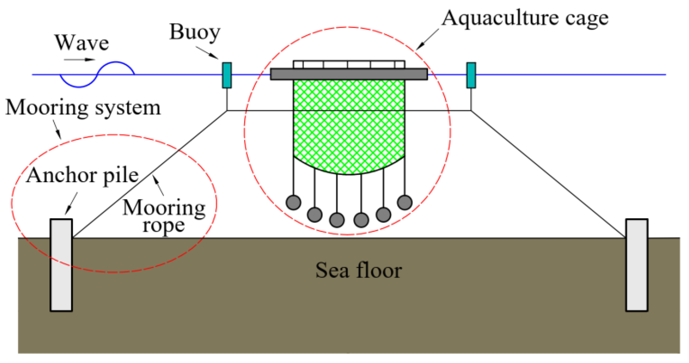
Offshore floating marine aquaculture, such as cage aquaculture and raft aquaculture (Figure 1), is an important part of China’s marine aquaculture industry, with a yield of 7153,265 tons in 2020, accounting for 33.4% of China’s total marine aquaculture output. Previous studies on aquaculture structures have paid more attention to the upper part of the floating body and analyzed the safety performance of the structure through a combination of numerical simulation, physical model experiments, and field investigation [1,2,3]. Xu et al. [4] presented the stress range of a mooring line based on the time domain analysis, and used the spectrum analysis method to analyze the fatigue analysis of the anchoring system. Hou et al. [5] used the time-varying method to analyze the sensitivity of the mooring line fatigue reliability to the random variable uncertainty under the fatigue limit state based on the S-N curve. However, even as an important part of floating marine aquaculture, the anchor member has seen less research on its uplift resistance. Cortes-Garcia et al. [6] used finite element analysis software to analyze the feasibility of applying screw anchors to aquaculture facilities and concluded that the suitable type of mooring profile in the screw anchor used for aquaculture is taut tension. Trujillo et al. [7] conducted experiments on different types of gravity anchors commonly used in raft aquaculture structures, and the results indicated that variable initial tension angles had considerable effects on the uplift resistance. Hou et al. [8] investigated the embedded anchor chain in aquaculture cages by using the lumped-mass method and showed that an embedded anchor chain has a significant impact on the retaining holding capacity of embedded anchors in a single-point mooring system. Therefore, the design and operation stages cannot be negligible.

Figure 1.
Floating net cage aquaculture system.
As a low-cost and easy-to-install anchor member, anchor piles are widely used in floating marine aquaculture. The tilt uplift load is the main stress on the anchor piles in practical aquaculture. Many researchers [9,10,11] have investigated the oblique uplift performance of piles under static loads through model experiments and proposed different methods to calculate the ultimate uplift load according to the failure form of soil around the pile. Clay is widely distributed in the offshore environment, so that mechanical properties must be considered in marine engineering design [12,13,14]. Gui et al. [15] used the fast load-keeping method to investigate the uplift resistance of anchor piles for marine aquaculture in clay. Floating marine aquaculture is usually subjected to low-frequency, long-term cyclic loads caused by wind, waves, and currents, as well as high-frequency cyclic loads caused by extreme weather such as typhoons and hurricanes. Compared with static loading, cyclic loading significantly reduces the uplift resistance of the anchor in the mooring system.
Poulos et al. [16] stated that, compared with static load experiments, there are three main problems of piles under cyclic loading that deserve more attention than static load tests: (1) the reduction in the strength or stiffness of the pile–soil interface, (2) the failure period number (number of cycles for piles to reach the failure standard) of the pile, and (3) the cumulative deformation law of the pile top. Considering the softening effect of soil, Fan et al. [17] established an elastic–plastic calculation model using the reduction in the strength or stiffness of the pile–soil interface as the main evaluation index of the dynamic response. It was found that, under the action of cyclic loading, the strength distribution of the soil around the uplift pile is uneven, reducing the bearing capacity. Hong et al. [18] studied the change in soil stiffness at the pile–soil interface through a series of centrifugal model tests and 3D finite element analysis and found that semi-rigid piles in clay behave as flexible piles or rigid piles under lateral cyclic loads. Due to the instability of soil, even after repeat experiments, the failure period number of the pile varies greatly and can only be used as an auxiliary evaluation index.
Lai et al. [19] and Jardine et al. [20] used cumulative displacement as the main evaluation index of dynamic response to compare one-way cyclic loading and two-way cyclic loading. It was found that the cumulative displacement of the pile top under unidirectional cyclic loading is large, and the failure to the soil around the pile is larger, so this can represent the most unfavorable situation. Under extreme weather, the direction of the marine floating aquaculture structure subjected to waves is usually fixed, and the anchor piles are mainly subjected to unidirectional loads. Taking the coastal area of Zhejiang Province, China as an example, the seabed soil is dominated by silt, which has the characteristics of high compression and flow plasticity, and it also contains a large amount of organic matter and humus sediments [21]. At present, there is no research on the dynamic response of piles and anchors in this clay. Therefore, analyzing the dynamic responses of piles and anchors for marine aquaculture under cyclic loading is of great significance to the safety of aquaculture structures.
In this paper, a laboratory model experiment is established. First, the ultimate uplift loads of anchor piles are determined by static loading, and then, according to the ultimate uplift loads, the dynamic responses of anchor piles under different loading amplitudes and initial tension angles by cyclic loading is investigated. The main research indicators in the experiment are the elastic displacement of the top of the anchor piles, the cumulative displacement of the top of the pile, the stiffness of the soil, etc., which provide a theoretical basis for the design and installation of the anchor in floating marine aquaculture.
2. Materials and Methods
2.1. Experimental Setup
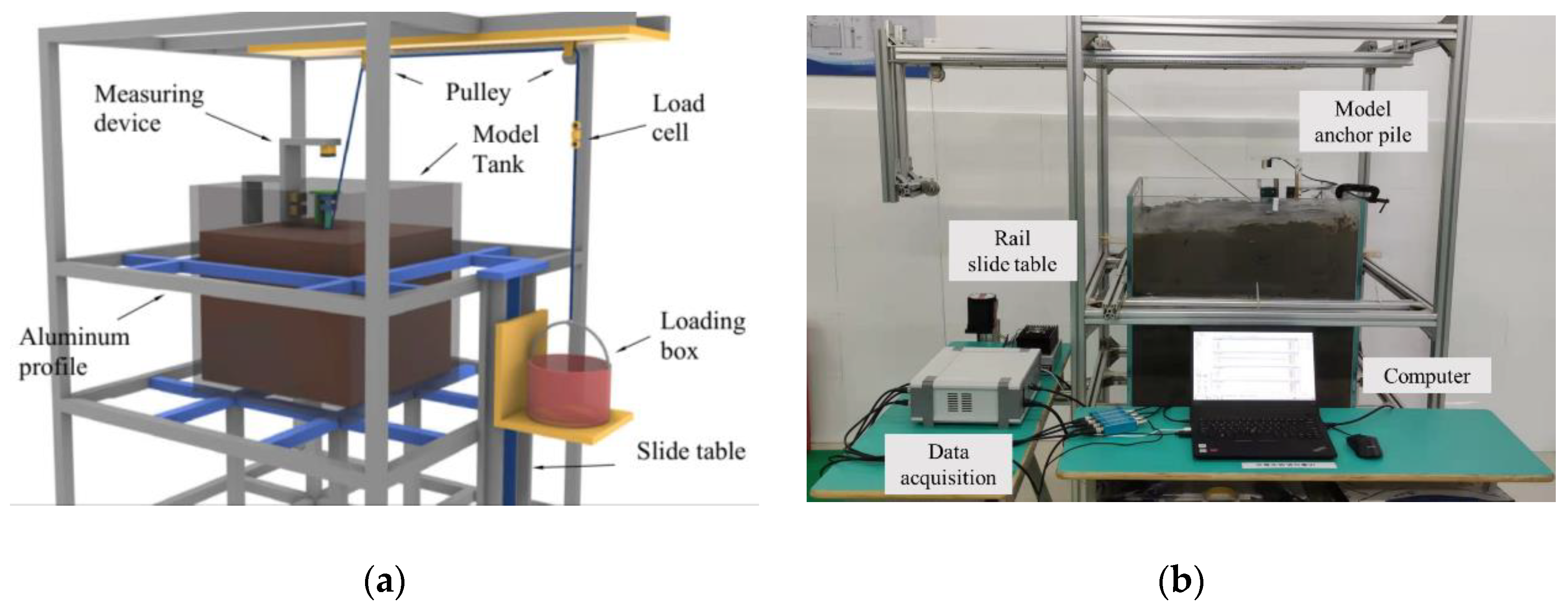
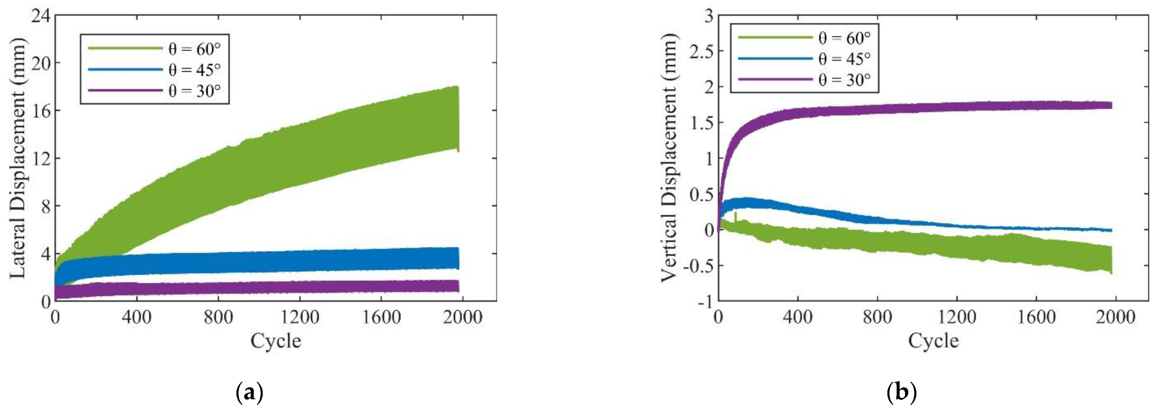
The experiments were conducted at the Marine Engineering Hydrodynamics Laboratory of the National Engineering Research Center for Marine Aquaculture, China. The experimental device was divided into four parts, namely the model box, frame system, loading system, and measurement system, as shown in Figure 2. The model box was made of 15 mm-thick glass, and the dimensions of the box were 700 mm × 700 mm × 700 mm. The model anchor piles were installed in the center of the experimental box, and the distance to the boundary was greater than 10 D (D is the diameter of the anchor piles; in this experiment, 1 D = 20 mm), which satisfied the boundary effect [22]. The frame system was made of aluminum profiles (section size: 40 mm × 40 mm), which mainly provided the reaction force for the model box. In addition, the aluminum profiles were deployed in the model box to make sure it was steady during the experiment.

Figure 2.
Schematic diagram (a) and photo (b) of the cyclic loading experimental setup.
2.2. Loading System
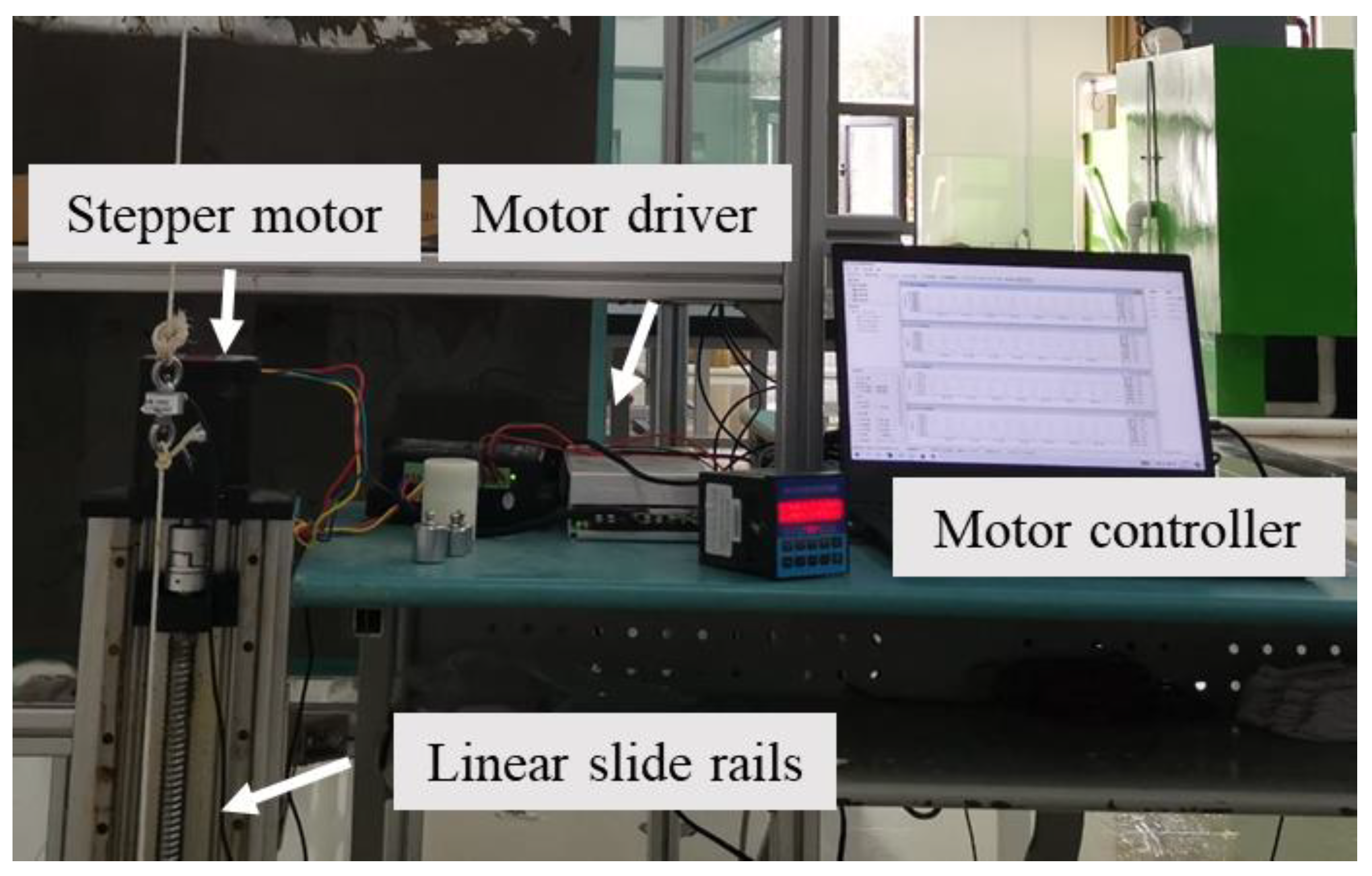
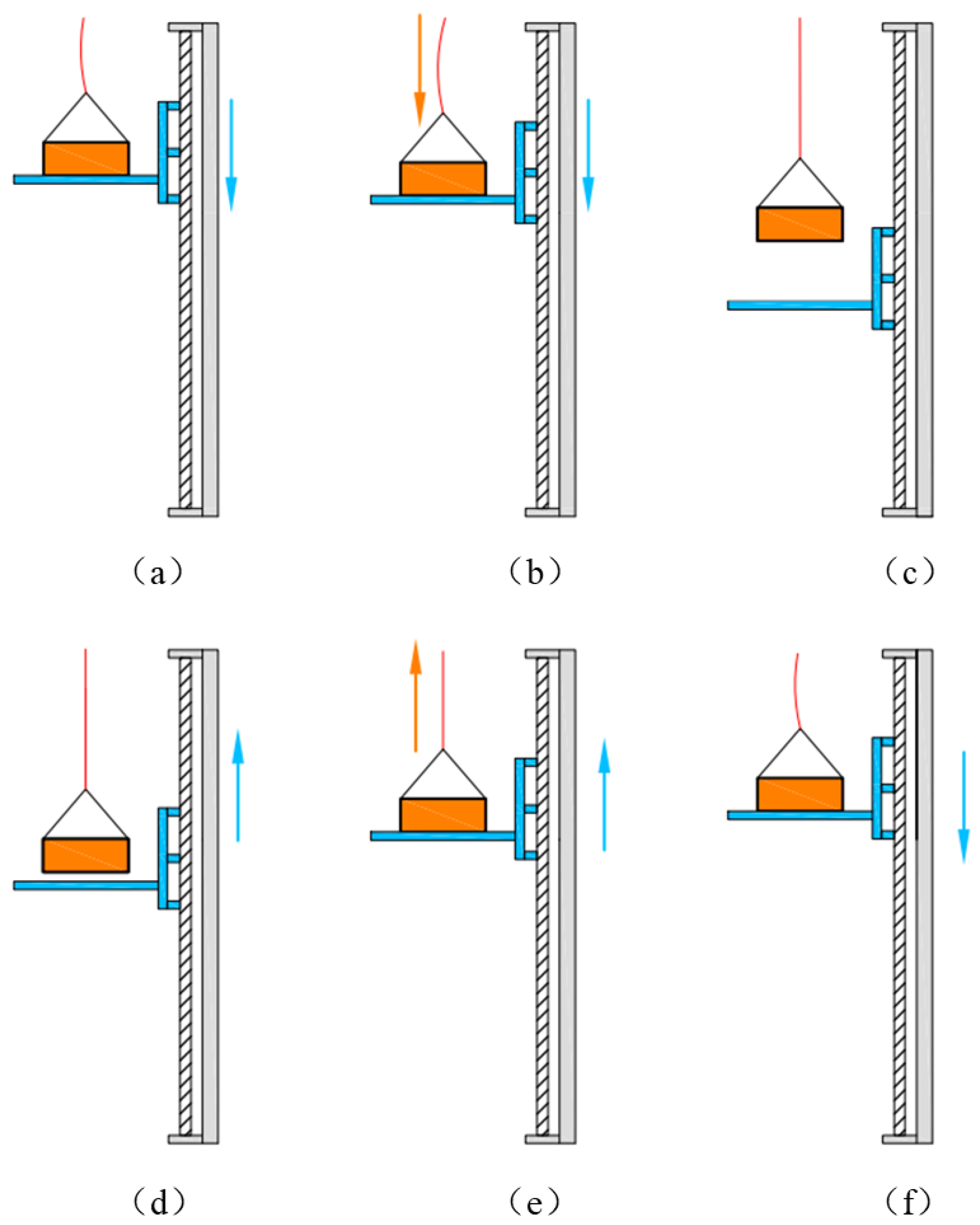
The main parts of the loading system were the pulleys, weights, loading box, and rail slides. As shown in the figure, two pulleys were needed in the experiment. Pulley 1 was fixed, and pulley 2 was movable to adjust the initial tension angle. The linear motion module sliding stepper is a device that can set the linear motion mode of the slider, which is mainly composed of the power supply, stepper motor, motor controller, motor driver, and other equipment (Figure 3). However, the maximum displacement of each reciprocating motion of the module was the same, consistent with the displacement control method in the cyclic loading method [23]. According to Lu et al. [24], the disadvantage of the displacement-controlled loading method is that the load output may decrease over time after the anchor piles generate cumulative displacement. Therefore, in order to ensure that the output load of the device remained consistent during the cyclic loading process, a loading device was designed in this paper that combined the loading box and the sliding table, as shown in Figure 4. The orange part is the loading box, and the blue part is the pallet support that fixed in the slider. The orange arrow is the movement direction of the loading box, and the blue arrow is the movement direction of the pallet support. A single load cycle was accomplished by this loading device as follows: At the stage of stand by (Figure 4a), the pallet was at the highest point, the loading box was supported by the pallet, the rope was slack, and the load was 0 N. After loading began (Figure 4b), the slider moved down, the support received by the loading box gradually decreased, and the output load gradually increased. When the slider moved to the lowest point (Figure 4c), the first half of the loading cycle ended, the loading box was completely suspended, and the output load reached the maximum value. Then, the pallet moved up from the lowest point (Figure 4d), and when it touched the loading box (Figure 4e), the loading box and the pallet rose at the same time, and the output load gradually decreased. When the slider moved to the highest point (Figure 4f), the loading box was fully supported, and the output load was reduced to 0 N. This completed a single load cycle.
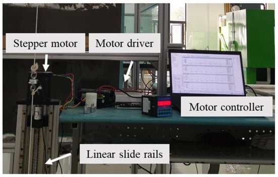
Figure 3.
Component of the linear motion module sliding stepper.
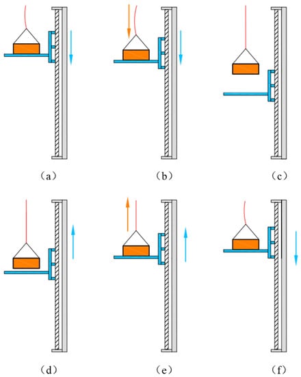
Figure 4.
Loading stage: pallet in the highest position (a), moving down (b), reaching the lowest position (c), moving up (d), touching the load box (e), and back to the highest position (f).
Figure 5 shows an example of the output load of the loading device. It can be seen from the figure that the load amplitude and frequency remained stable with the running time, indicating that the loading device meets the requirements of this experiment. During the loading process, a dynamic effect occurs at the initial stage of separation between the pallet and the loading box, which causes the output load to be unstable. After the weight box is completely suspended, the dynamic effect weakens and the output load returns to stable.
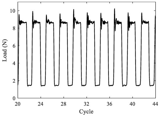
Figure 5.
Example of output load of the loading device.
2.3. Model Anchor Piles and Clay
In this experiment, the anchor pile model was mainly affected by oblique tension, and the geometric similarity and force field similarity were mainly considered when making the anchor pile model [25]. The main parameters of the prototype and the model must satisfy the following formula:
where , , and are the characteristic length, elastic modulus, and section moment of inertia of the prototype structure, respectively, and , , and are the characteristic length, elastic modulus, and section moment of inertia of the model structure, respectively. is the proportionality constant. In this paper, = 1:7 was selected, and the model anchor piles were made of a plexiglass tube with a wall thickness of 2 mm. The flexural stiffness of the model anchor piles was determined by a simple cantilever beam experiment. The empirical calculation conforms to Formulas (1) and (2). The specific parameters are shown in Table 1.

Table 1.
Model anchor pile parameters.
The clay used in the experiment was taken from Changzhi Island, Zhoushan, Zhejiang Province, China. Before the experiment, it was necessary to screen out the impurities in the clay sample, add water, and stir to fully saturate the clay sample. After the clay samples were processed, the following specific parameters were measured (Table 2).
Table 2.
Clay parameters.
2.4. Measurement System
During the experiment, the model anchor piles were displaced in both the lateral and vertical directions due to the oblique load. According to the experimental method of Shin et al. [9], three laser displacement sensors (LDS, Chengdu Xinda Shengtong Technology Co., Ltd., Chengdu, China. range: 0–30 mm, accuracy: 0.1%) were used to collect displacement data (Figure 6). LDS #1 and #2 were used to measure the horizontal displacement, and LDS #3 was used to measure the vertical displacement. The laser displacement device measured the distance through the time interval of total reflection after hitting the target object. The reflection ability of the measured object determines the reliability of the measurement data. In this experiment, the model anchor piles had a circular section, which affects the reflection ability of the laser, leading to measurement uncertainty. A square plastic clamp was sleeved on the outside of the model anchor pile, so that a square section was formed, and an acrylic plate was pasted on the outside of the square clamp. This can expand the contact area between the laser emitted by the sensor and the model anchor pile, ensuring the accuracy of the measurement. In the experiment, a load cell (Chengdu Xinda Shengtong Technology Co., Ltd., Chengdu, China range: 0–200 N, accuracy: 0.1%) was used to obtain tension data. The synchronous acquisition of LDS and load cell data was realized through the data hub (Chengdu Xinda Shengtong Technology Co., Ltd., Chengdu, China, product model: UBK-16). In this experiment, the load cell measured a load of 1.7 N due to its own weight; therefore, the minimum value of the load cell during the experiment was not 0 N (Figure 5).
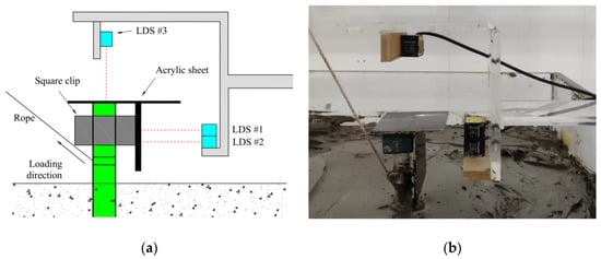
Figure 6.
Schematic diagram (a) and photo (b) of the measurement system.
2.5. Test Conditions
According to the monitoring results of Yin et al. [26] and Wu et al. [27] in the sea, the wave period was usually about 5~9 s, and here we choose 6.3 s () as the prototype for the wave period for the following analysis. According to the similarity theory, the time parameter of wave period in the experiment ( and that in the prototype should satisfy the following formula.
where λ is the similarity ratio. In this study, λ = 1:7, so the loading period in the experiment should be 2.37 s. Usually, the effects of a red-level hurricane will last for 3 to 4 h. Thus, the maximum number of cycles was set to 2000, which is equivalent to 3.5 h of cyclic loading in the real sea. The main experimental steps in this paper were as follows: (1) Fill the reshaped clay in the model box, and evenly distribute it by stirring continuously. (2) Install the model anchor piles at the designed depth of the clay, and be careful not to affect the clay around the pile during installation. (3) Install the measurement system and start cyclic loading. (4) Stop loading after the cycle is ended or the model anchor piles are completely pulled out and end the experiment.
A total of 13 groups of experiments (Table 3) were set up in this paper, which can be divided into two types: static experiments and dynamic experiments. Conditions 1–4 were static experiments, aiming to determine the ultimate uplift capacity of the anchor piles. Cases 5–8 investigated the effect of the loading amplitude on the uplift resistance of the anchor piles under vertical cyclic loading conditions. Cases 9–11 investigated the effect of the variable initial tension angle on the uplift resistance of the anchor piles under oblique cyclic loading. Cases 10, 12, and 13 mainly investigated the effect of the cyclic loading amplitude on the uplift capacity of the anchor piles with a constant tension angle of 45°. The main range of the initial angle was 30°~60° when investigating the oblique force of the anchor member, so the initial tension angle was selected as 30°, 45°, and 60° in this study. The pre-experiment showed that the anchor piles may be damaged when (load cycle amplitude) = 0.6~1.0. When the load amplitude is too low, the dynamic response of the anchor piles is basically the same. Therefore, = 0.6, 0.8, 0.9, and 1.0 are selected for the vertical experiments, and 0.6, 0.8, and 1.0 for the oblique experiments.
Table 3.
Test conditions.
3. Results and Discussion
3.1. Ultimate Uplift Resistance of Anchor Piles under Static Loads
The ultimate pull-out load of the model pile anchors was determined by static tests before the cyclic test. Referring to the research of Gui et al. [15], this research adopted the rapid curing load method to carry out the test. This involved gradually increasing the load and recording the displacement of the model pile anchor after a certain time under different loads, so as to obtain the displacement–load relationship. Generally, there were many ways to determine the ultimate pull-out load, e.g., setting the maximum displacement generated at the top of the pile anchor, deflection, or based on the displacement–load curve, etc. [28]. In this test, when the total displacement of the top of the pile anchor exceeded 0.15 D (D is the diameter of the pile), the pile anchor was considered in the condition of damaged. The experimental results showed that the ultimate lifting loads () of θ = 0°, 30°, 45°, and 60° were 13.4 N, 16 N, 21.5 N, and 23.5 N, respectively.
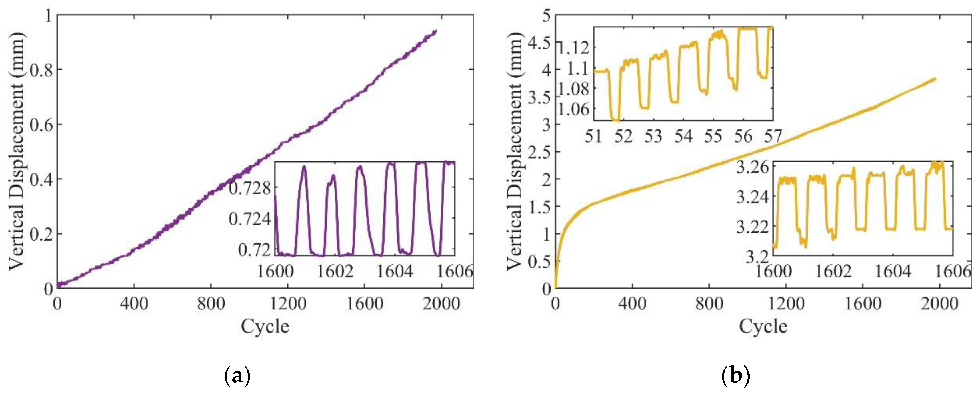
3.2. The Effect of Vertical Loading Amplitude
Four groups of a load amplitude of = 0.6, 0.8, 0.9, and 1.0 with vertical cyclic loading were set to explore the influence of the vertical load amplitude on the uplift resistance capacity. Figure 7 shows the time history of the displacement with variable loading amplitudes under vertical cyclic loading. The x-axis in the figure is the number of load cycles, and the y-axis is the vertical displacement of the top of the model anchor piles. It can be seen from the figure that the cumulative displacements generated by variable loading amplitudes, and the displacements generated by the pile top in a single cycle both were different. The displacement generated in the cyclic loading can be divided into two categories [29]: The first is elastic displacement, the displacement generated when the load increases in a single cycle, and the displacement disappears when the load decreases. The magnitude of the elastic displacement is related to the stiffness of the clay. The other type is cumulative displacement, which is permanent displacement caused by an increase in loading time during the loading process. Cumulative displacement is related to the plastic deformation of the clay.

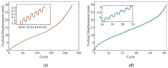
Figure 7.
Time history of displacement of vertical cyclic loading with variable loading amplitudes: (a) = 0.6, (b) = 0.8, (c) = 0.9, (d) = 1.0.
Jardine et al. [20] summarized three types of motion characteristics of anchor piles under cyclic loads: (1) Stable: under unidirectional or bidirectional loads, the displacement of the pile top slowly accumulates over hundreds of cycles. (2) Unstable: under one-way or two-way loads, the displacement develops rapidly, resulting in failure when the number of cycles is less than 300. (3) Metastable: the pile head displacement accumulates at a moderate rate within tens to hundreds of cycles, and fails when the accumulated displacement reaches a certain value. According to the above research conclusions, this research will analyze the uplift resistance of anchor piles under different test conditions, considering three aspects: the cumulative displacement change trend, the soil stiffness degradation, and the number of cycles at destruction.
Figure 7a shows the result of loading amplitude = 0.6. It can be seen from the figure that the growth rate of the cumulative displacement during the loading process is basically the same, and the final cumulative displacement is 0.9 mm after two thousand loadings. Figure 7b shows that the result of the loading amplitude is = 0.8. The anchor piles were not pulled out during the loading process, but an obvious cumulative displacement was generated. The cumulative displacement growth rate was fast in the initial stage and then became slow. The first 400 cycles produced a cumulative displacement of 1.5 mm, and in the last 1600 cycles, the cumulative displacement increased by 2.3 mm. After 2000 cycles, in case of = 0.6 and 0.8 the anchor piles were not pulled out, but the displacement development mode and the final cumulative displacement were different in these two cases. This indicates that when the cyclic loading amplitudes were = 0.6 and 0.8, the anchor piles could still remain stable after loading for 3.5 h in actual marine aquaculture. Figure 7c,d are the experimental results of the loading amplitudes = 0.9 and 1.0, respectively. It can be seen from the figure that the displacement development trend of the two working conditions under the action of cyclic loads are similar. The pile top displacement increases with the increase in the number of cycles, and the cumulative displacement growth rate first decreases and then increases. It can be seen from the subfigure in Figure 7c,d that the preset maximum displacement is reached when N (number of cycles) = 285 and 85 times, and the model anchor pile is considered to be pulled out. This shows that in the actual marine aquaculture environment in regular wave loading, when the cyclic load amplitudes are = 0.9 and 1.0, the anchor piles will fail after 30 min and 9 min, respectively.
It can also be seen from the subfigure in Figure 7 that when N = 1600, the elastic displacement of = 0.6 was about 0.006 mm, and the elastic displacement of = 0.8 was about 0.040 mm. When N = 60, the elastic displacement of = 0.9 was about 0.12 mm. When N = 16, the elastic displacement of = 1.0 was about 0.17 mm. As the loading amplitude increased, the elastic displacement generated by the anchor piles increased significantly. Compared with = 0.6, the elastic displacement of = 0.8 was improved by about seven times, but the improvement effect was obviously reduced as the loading amplitude increased.
Cheng et al. [30] considered that the stiffness of soft clay decreases under cyclic loading, and the degree of this stiffness degradation is related to the influence of many factors, such as the number of cycles, the magnitude of the initial tensile force, the loading amplitude, and the consolidation ratio. The generation of cumulative displacement under cyclic loading is mainly caused by the degradation of soil stiffness, which refers to the ratio of the maximum and minimum load difference to the displacement difference in each cycle in the following formula:
where is the i th cycle, is the maximum tensile load on the anchor piles in a single cycle, is the minimum tensile load on the anchor piles in a single cycle, is the maximum displacement in a single cycle, and is the minimum displacement in a single cycle.
In order to investigate the effect of loading amplitude on stiffness, the soil stiffness values at N = 20 in four groups of test conditions were calculated, and the results are shown in Table 4. It can be seen from the table that the soil stiffness gradually decreased with the increase in the vertical loading amplitude, and the soil stiffness of = 0.6 was the largest, which is 93% lower than that of = 0.8. The soil stiffness of = 1.0 was the smallest, and the stiffness values of = 0.8, = 0.9, and = 1.0 were relatively similar. This shows that the stiffness of the clay in the steady state is greater than that in the other states.
Table 4.
Soil stiffness under vertical loading with different loading amplitudes (N = 20).
3.3. The Effect of Initial Tension Angle
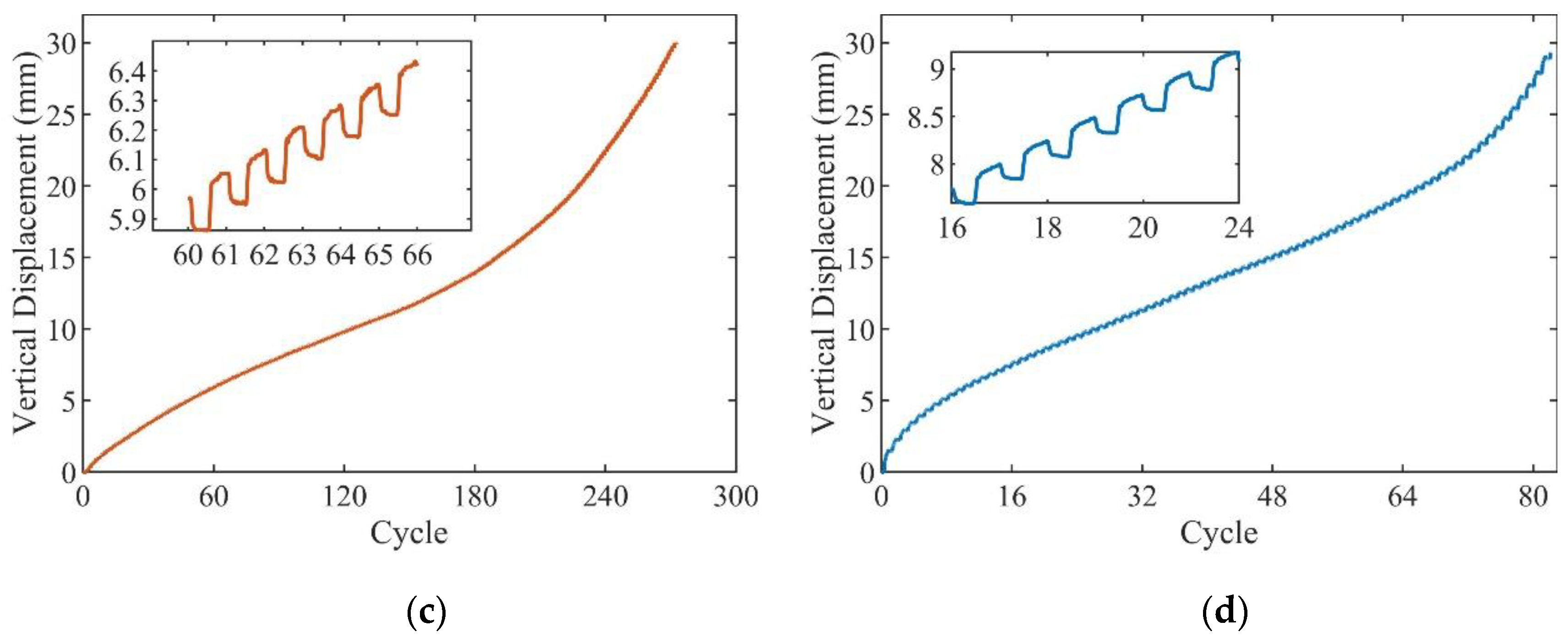
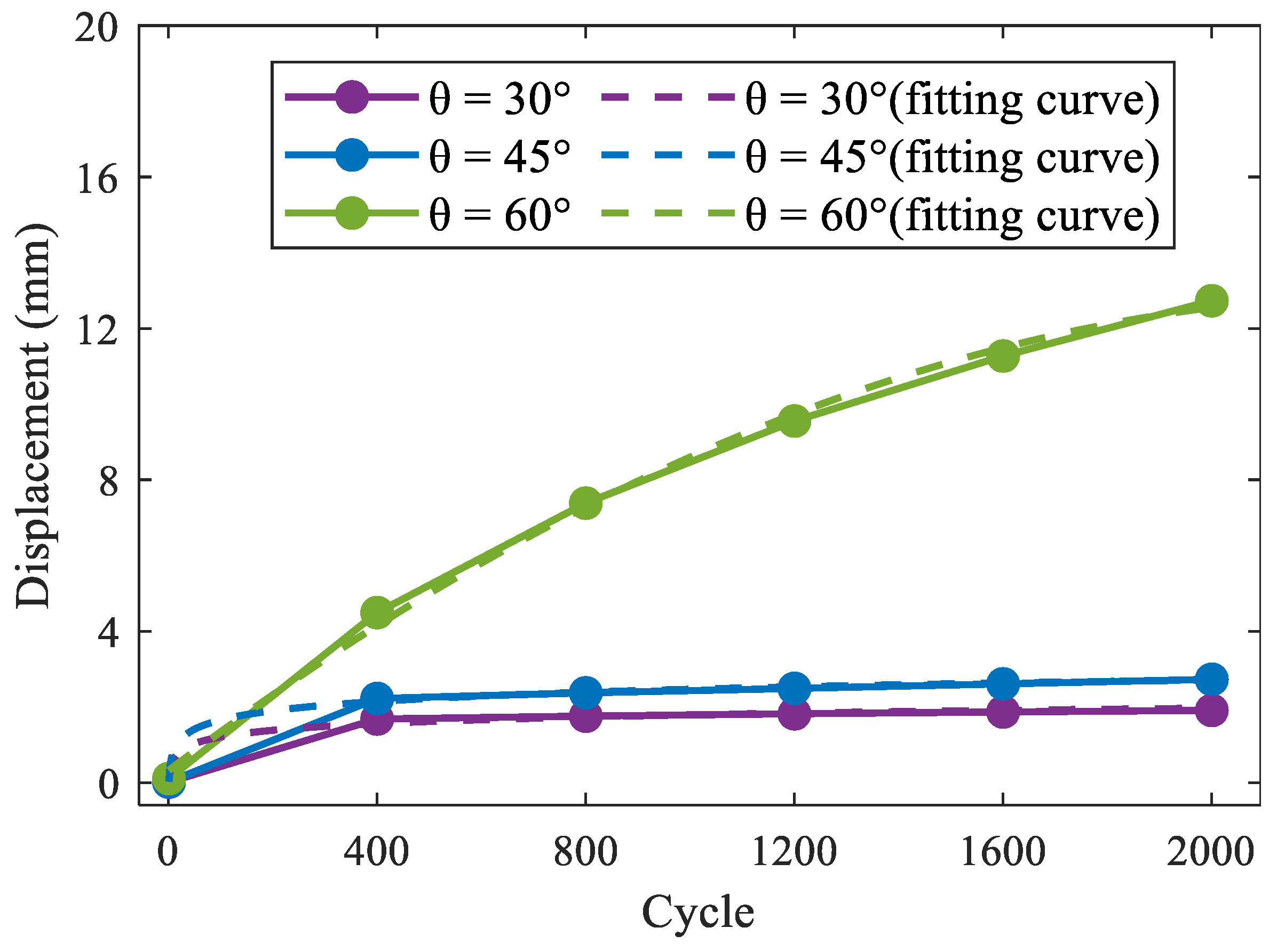
Three groups of initial tension angles of 30°, 45°, and 60° with a uniform loading amplitude of 13 N were set to explore the influence of the initial tension angle on the uplift resistance capacity. Figure 8a show the time history curve of the lateral displacement with variable initial tension angles under oblique cyclic loading. It can be seen from the figure that the lateral displacement of the clay increased with the increase in the initial tension angle, and the cumulative displacements after 2000 cycles were 0.85, 2.76, and 12.86 mm, respectively. This may be due to the increased lateral component force of the anchor pile when θ = 60°, but the lateral bearing capacity of the clay is weak, resulting in significant cumulative displacement [15]. In addition, it can be seen from the figure that the elastic displacement in the lateral direction increases with the increase in the initial tension angle.

Figure 8.
Time history of displacement of cyclic loading with variable initial tension angles: (a) lateral, (b) vertical.
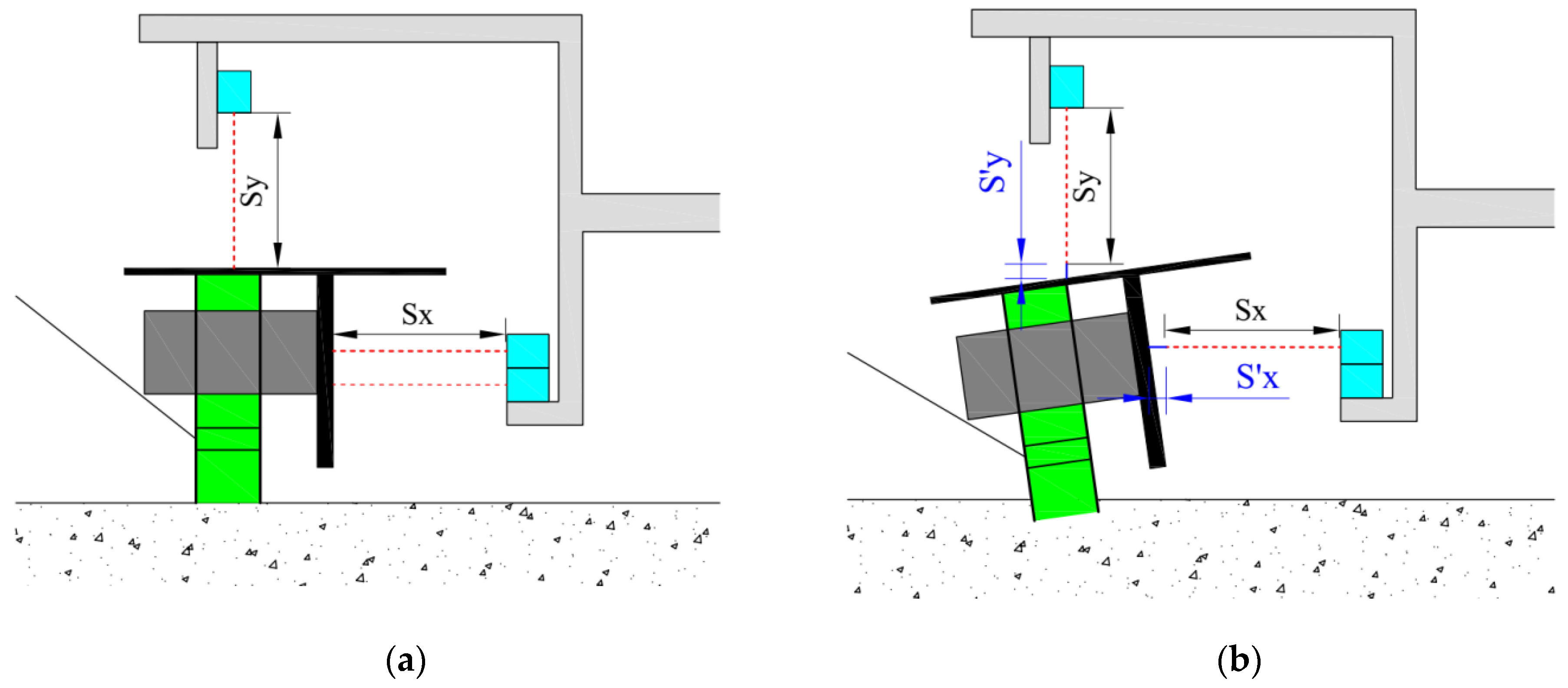
Figure 8b shows the time history of the vertical displacement with variable initial tension angles under oblique cyclic loading. The vertical displacement characteristics under variable tension angles were different. The displacement at θ = 30° gradually increased, the displacement development rate first increased and then decreased in two stages, and the final cumulative vertical displacement was 1.78 mm. The displacement at θ = 45° firstly increased and then decreased, and the final cumulative vertical displacement was –0.02 mm. The displacement at θ = 60° always decreased, and the final cumulative displacement was –0.58 mm. Negative displacement in the vertical direction means that the measured object moves away from the laser displacement sensor; that is, the anchor piles move downward. The reason for the negative displacement in the test may be the deflection of the anchor pile. The reason for the negative displacement in the test may be the deflection of the anchor pile. As shown in Figure 9, in the initial state, the lateral and vertical displacements of the anchor piles are Sx and Sy respectively when the action of the load. After cyclic loading, the deflection deformation occurs. the anchor piles was far away from the sensor, resulting produce the displacement S’x and S’y.
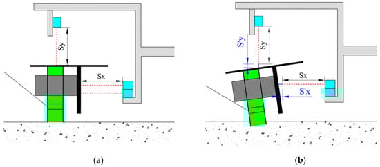
Figure 9.
Deformation of anchor piles under oblique loading: (a) before deflection, (b) after deflection.
As displayed in Figure 9, the reason for the negative displacement in the experiment may lie in the deflection of the anchor piles in the process of generating the cumulative displacement, and the deflection did not change with the change in the load. When the load was reduced, the anchor piles returned to their initial position, the acrylic plate was tilted due to the deflection, and the original measurement position was far away from the sensor, resulting in a displacement in the opposite direction.
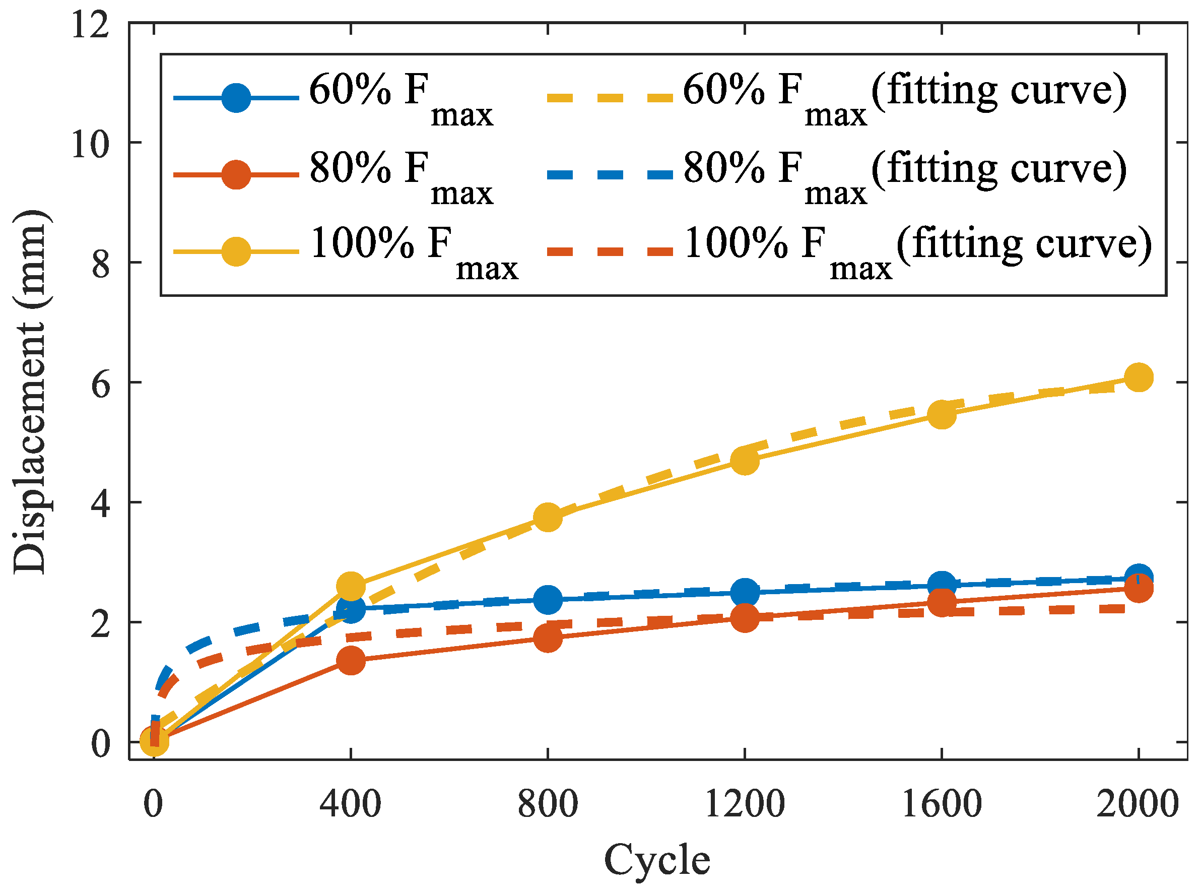
Bai et al. [31] considered that the relationship between the number of loads and the cumulative displacement can determine whether the anchor pile is in a stable state: the curve in the stable state should satisfy the logarithmic function relationship, and the curve in the unstable state should satisfy the power function relationship. Combine the lateral cumulative displacement and the vertical cumulative displacement into the total cumulative displacement, and draw a load-total cumulative displacement relationship curve (Figure 10). It can be seen from the figure that the cumulative displacements of the first 400 cycles of the three sets of test conditions were 1.68, 2.22, and 4.49 mm, accounting for 88%, 81%, and 35% of the overall cumulative displacement. This shows that the cumulative displacements of θ = 30° and θ = 45° were mainly generated in the first 400 cycles, and then the cumulative displacement development gradually stabilized. When θ = 60°, the accumulated displacement was mainly generated in the last 1600 cycles and will continue to increase.
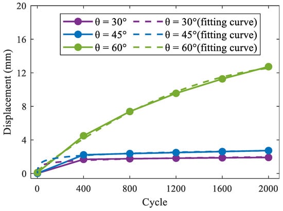
Figure 10.
Cycle times–cumulative displacement relationship for variable initial tension angles.
Table 5 shows the fitting functions of the cumulative displacement for variable initial tension angles. The fitting functions of θ = 30° and θ = 45° were closer to the logarithmic function, and the fitting functions of θ = 60° were closer to the quadratic polynomial. The growth rate of this function is obviously greater than that of the logarithmic function and less than that of the power function, so it can be considered a metastable state.
Table 5.
Cumulative displacement fitting function for variable initial tension angles.
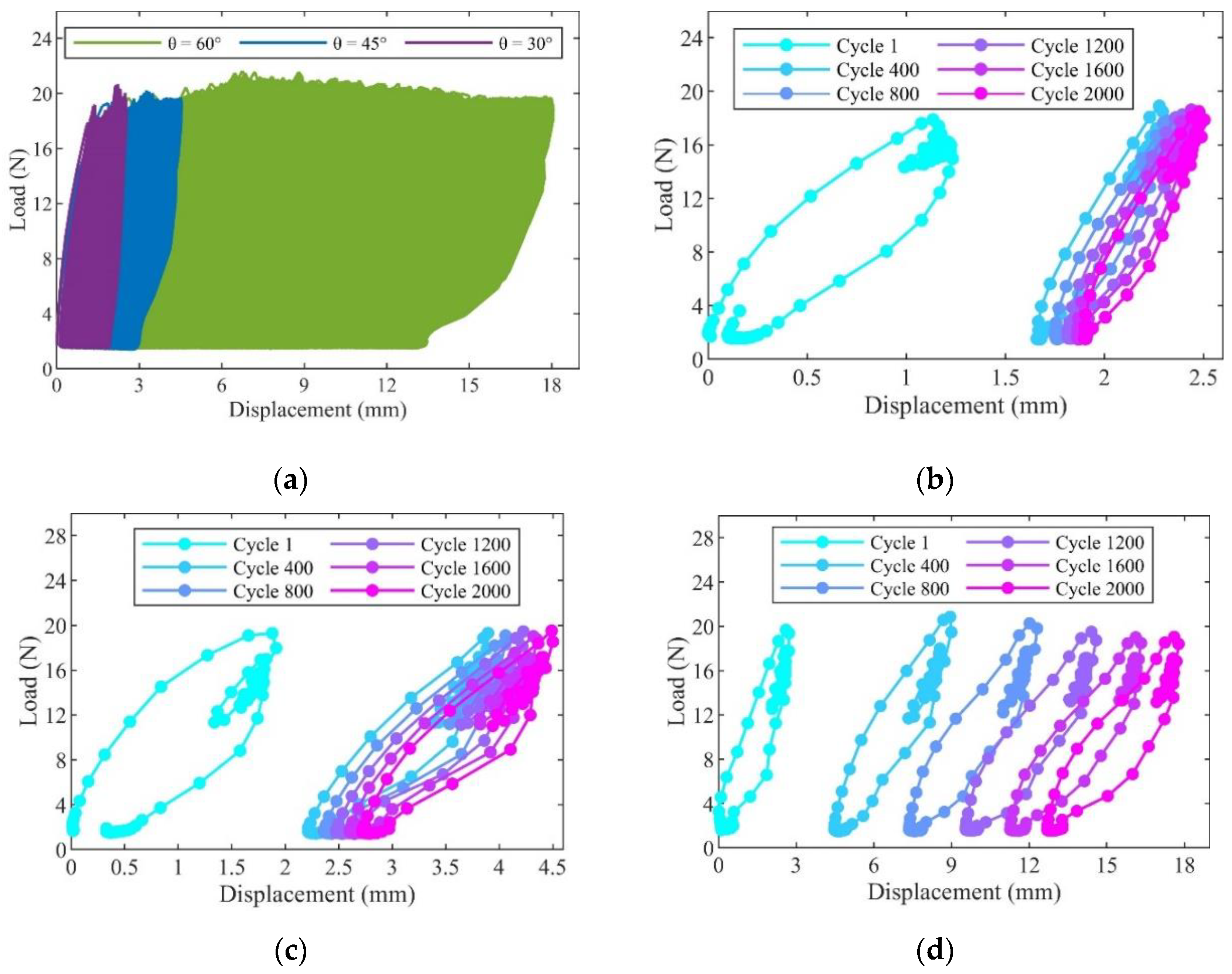
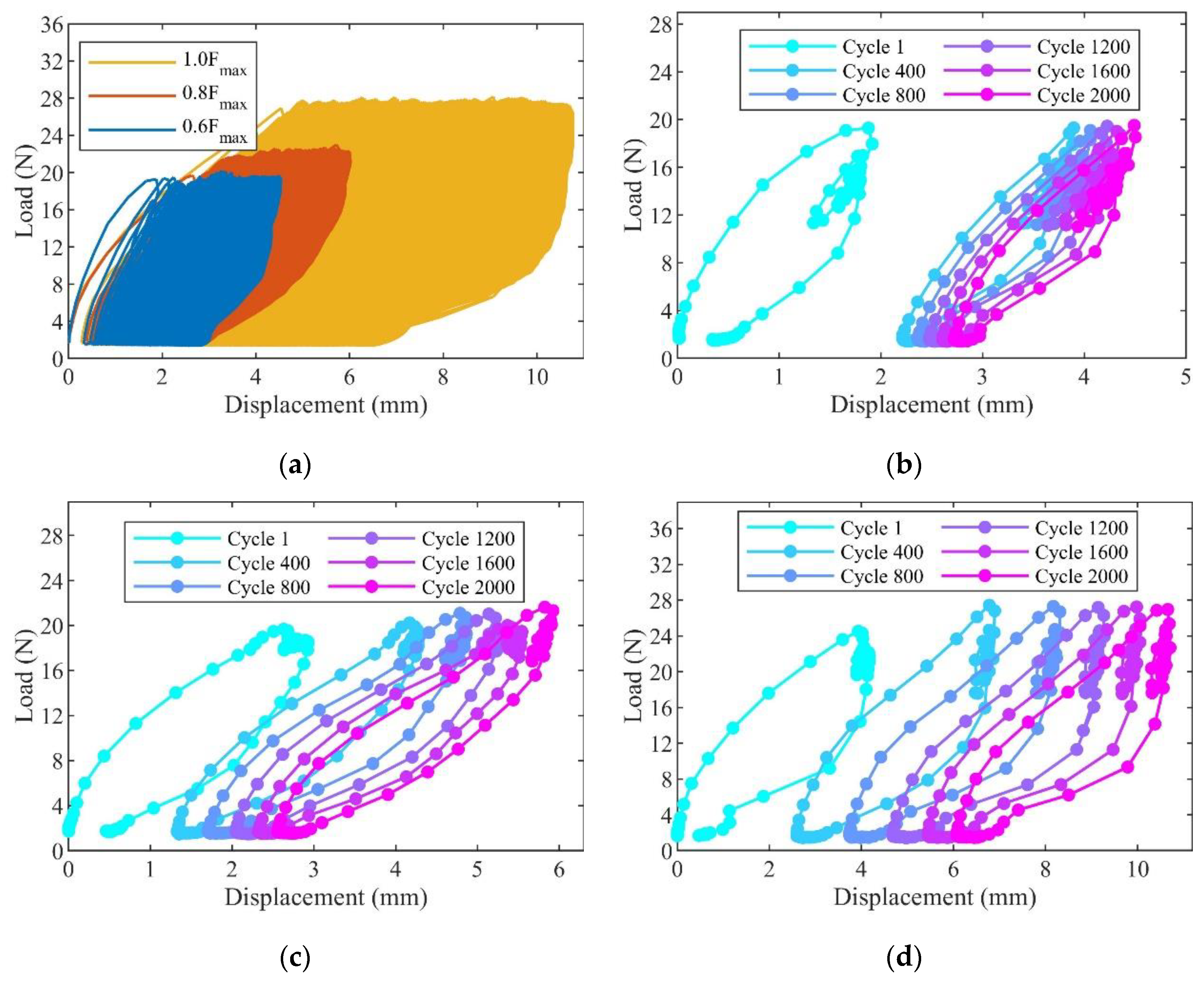
The load–displacement hysteresis curves of the three groups of initial tension angles have been depicted in Figure 11a. It can be seen from the figure that the curve area with θ = 60° was the largest, and the area with θ = 30° was the smallest. In order to facilitate the analysis, the hysteresis curves of N = 1, 400, 800, 1200, 1600, and 2000 under each group of test conditions were drawn, and the change law of the movement mode of the anchor piles during the experiment was investigated.
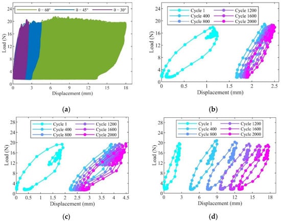
Figure 11.
Displacement load hysteresis curves under variable tension angles: (a) total; (b) θ = 30°; (c) θ = 45°; (d) θ = 60°.
The hysteresis curve at θ = 30° was shown in Figure 11b and accurately reflected the movement mode of the anchor piles [32]. The hysteresis curve of each cycle consists of two parts: loading and unloading. Generally, the load curve is convex during the loading stage, and the hysteresis curve of the clay is concave during unloading. After the load of the loading stage in the figure reaches the maximum value, multiple data points shift or even rebound, which is caused by the output load of the loading device (Figure 5). As can be obviously seen that the movement mode of the anchor piles was the most special when N = 1. The loading stage is a smooth convex curve, and the unloading stage is a smooth concave curve. At this time, the area of the hysteresis loop was the largest, and the first loading produced a large cumulative displacement. This phenomenon has appeared in many experiments [33]. The movement modes of the anchor piles for the rest of the cycles were similar; the loading and unloading stage had smooth curves, the slope of the curve was significantly higher than that when N = 1, and the area of the hysteresis loop was basically the same.
Figure 11c shows the displacement–load hysteresis curve under the cyclic load at θ = 45°. It can be seen from the figure that the movement characteristics of the anchor piles were special when N = 1, and the curve of the unloading stage showed a rebound phenomenon and the area enclosed by the hysteresis loop was the largest. For the rest of the cycle times, the movement of the anchor piles was similar, and the area of the hysteresis loop was similar. Figure 11d is the displacement–load hysteresis curve under the cyclic load at θ = 60°. It can be seen from the figure that, unlike the other two groups of tension angles, the hysteresis loop area of the hysteresis curve when N = 1 was the smallest. As the number of cycles increased, the slope of the loading end curve gradually decreased. This shows that the soil stiffness gradually decreased, and the bearing capacity of the clay will decrease accordingly [30]. After continuing to load for a period of time, the clay will be damaged. At this time, the model anchor pile is in a metastable state.
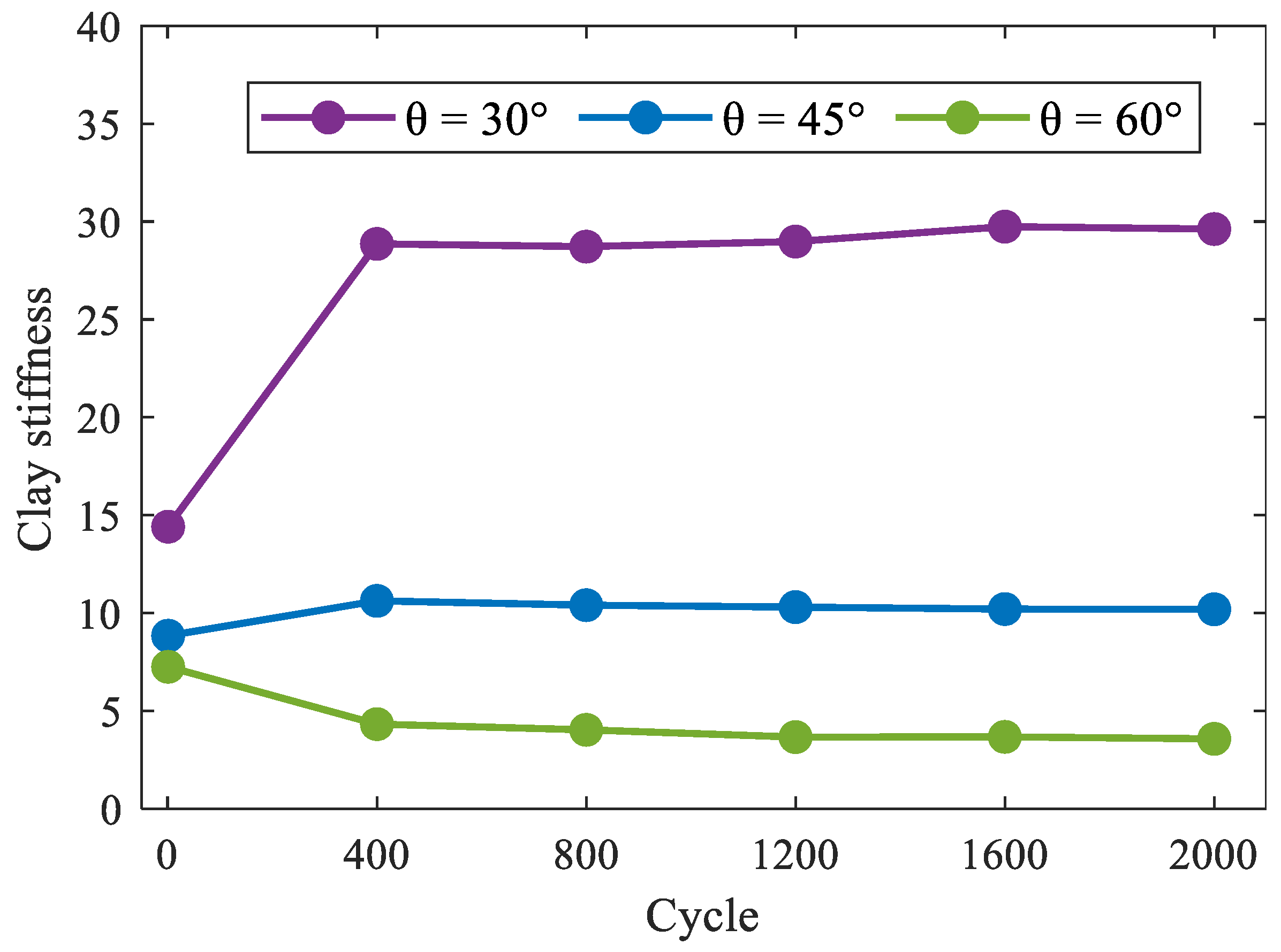
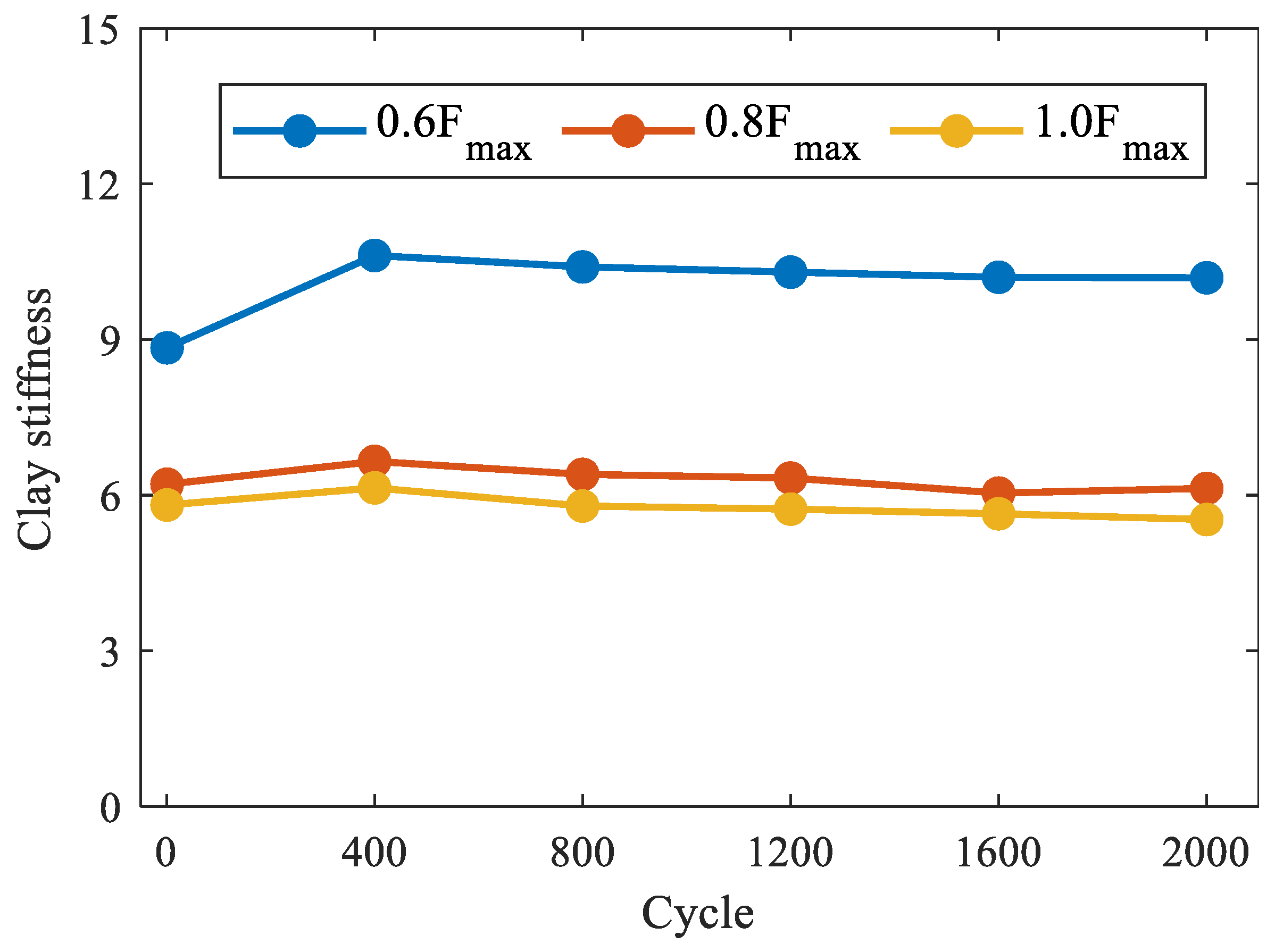
The degradation of soil stiffness under variable initial tension angles have been shown in Figure 12 and the soil stiffness gradually decreased with the increase in the tension angle. When N = 400, the soil stiffness of θ = 30° was 2.71 times and 6.67 times that of θ = 45° and θ = 60°, respectively. With the increase in the number of cycles, the soil stiffness at θ = 30° increased gradually, and the increase in the soil stiffness was the largest in the first 400 cycles. The soil stiffness in the case of θ = 45° first increased and then decreased, and the variation range of the stiffness during loading was smaller than that in the case of θ = 30°. The soil stiffness at θ = 60° gradually decreased, and the decrease was the largest in the first 400 cycles.
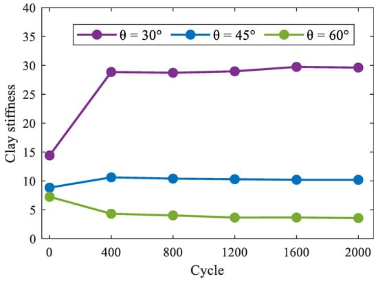
Figure 12.
Variation in soil stiffness under cyclic loading with variable initial tension angles.
After 2000 cycles, the anchor piles under three groups of different tension angles were not pulled out. Through the analysis of angles such as lateral and vertical displacement change, cumulative displacement change trend, hysteresis curve and stiffness degradation of anchor piles, it can be concluded that the θ = 30° and θ = 45° were stable states, and the θ = 60° was a metastable state.
3.4. The Effect of the Oblique Loading Amplitude
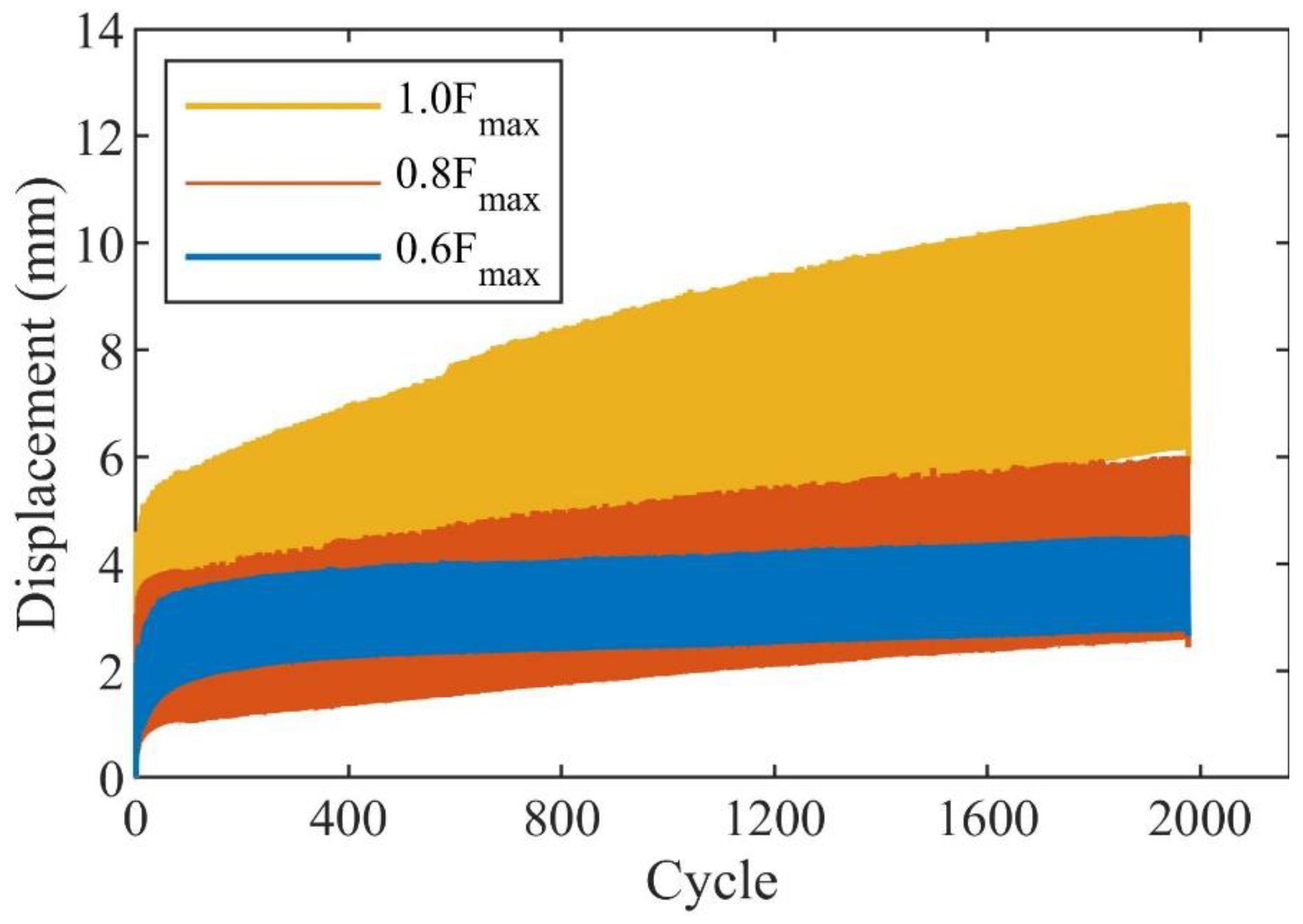
Three groups of load amplitude of = 0.6, 0.8, and 1.0 with a uniform initial tension angle θ = 45° were set to explore the influence of the oblique load amplitude on the uplift resistance capacity. Figure 13 shows the time history of the total displacement with variable initial loading amplitudes under oblique cyclic loading. As shown in the figure, with the increase in the loading amplitude, the elastic displacement of the top of the anchor piles increased.

Figure 13.
Time history of the displacement of variable cyclic loading amplitudes (θ = 45°).
The relationship between the number of cycles and the cumulative displacement for variable cyclic loading amplitudes at θ = 45° is shown in Figure 14. It can be seen from the figure that the accumulation of the first 400 cycles of the three groups of test conditions was 2.22 mm, 1.36 mm, and 2.597 mm, accounting for 81%, 53%, and 42% of the final cumulative displacement, respectively. This indicates that the cumulative displacements of = 0.6, 0.8, and 1.0 were mainly generated in the first 400 cycles. With the increase in the loading amplitude, the proportion of the cumulative displacement generated in the first 400 cycles gradually decreased, and the cumulative displacement generated in the subsequent cycles gradually increased. The final cumulative displacement of = 0.8 was less than = 0.6. According to the trend of cumulative displacement, if the loading continues, the final cumulative displacement of = 0.8 will exceed = 0.6. Table 6 shows the fitting functions of the cumulative displacements at variable loading amplitudes. The fitting functions of = 0.6 and = 0.8 were closer to the logarithmic function and were in a relatively stable state. The = 1.0 fitting function was closer to a quadratic polynomial and was in a metastable state.
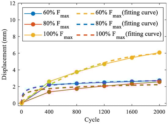
Figure 14.
Cycle times-cumulative displacement relationship for variable loading amplitudes (θ = 45°).
Table 6.
Cumulative displacement fitting function for variable loading amplitudes (θ = 45°).
The load–displacement hysteresis curves under variable oblique loading amplitudes at θ = 45° is displayed in Figure 15a. It can be obviously seen that the = 1.0 test condition had the largest curve area, and the = 0.6 test condition had the smallest curve area. Figure 15b is the displacement-load hysteresis curve under the cyclic load for = 0.6, which has been described in detail above. Figure 15c is the displacement-load hysteresis curve under the cyclic load for = 0.8. It can be seen from the figure that the movement modes of the anchor piles under variable cycle times are basically the same, and the curves of the loading stage and the unloading stage are smooth. When N = 1, the area of the lag loop was slightly larger than the number of other cycles. Figure 15d shows the displacement–load hysteresis curve under cyclic loading for = 1.0. It can be seen from the figure that when N = 1, the curve of the unloading stage had an obvious turning point, and the area of the hysteresis loop was the largest at this time. For the rest of the cycles, the movement patterns of the anchor piles were similar, and the curve of the loading end was convex at first and then concave, but the area of the hysteresis loop was basically the same.
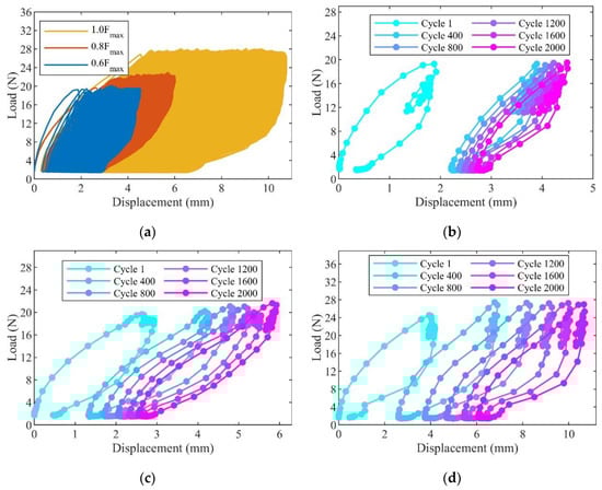
Figure 15.
Variable loading amplitudes displacement–load hysteresis curve (θ = 45°): (a) total, (b) = 0.6, (c) = 0.8, (d) = 1.0.
Figure 16 depicted the degradation of soil stiffness under variable loading amplitude angles of θ = 45°. It can be seen from the figure that the soil stiffness of = 0.6 is significantly greater than that of = 0.8 and 1.0. As the loading amplitude increased, the soil stiffness gradually decreased. In addition, with the increase in the number of cycles = 0.6, the soil stiffness first increased and then decreased. The stiffness increased for the first 400 cycles and gradually decreased for the last 1600 cycles. When = 0.8 and 1.0, the soil stiffness changes were almost the same; they both increased first and then decreased, and the overall change range was small.
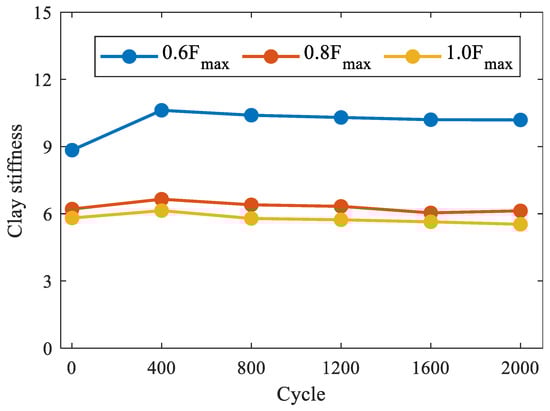
Figure 16.
Variation in soil stiffness under cyclic loading with variable loading.
After 2000 cycles, the anchor piles of the three groups of different loading amplitudes were not pulled out. Through the analysis of the elastic displacement change, cumulative displacement change trend, hysteresis curve, and stiffness degradation of anchor piles, it can be considered that = 0.6 and 0.8 is a stable state, and = 1.0 is a metastable state.
4. Conclusions
In this research, the influence of loading amplitude, initial tension angle, and other influencing factors on the anchor pile uplift resistance of marine aquaculture was investigated by conducting experiments under cyclic loading, and the following conclusions were drawn:
Anchor piles under the action of vertical cyclic load, the loading amplitude increases, the displacement of the top of the model anchor pile increases, and the stiffness of the soil around the pile decreases (N = 20). After 2000 times of loading, the anchor pile under = 0.6 and 0.8 was not pulled out, that is, the anchor piles was not damaged after the prototype structure was subjected to cyclic loading for 3.5 h. = 0.9 and 1.0 were pulled out after 285 and 85 cycles, respectively, i.e., the prototype structure failed after 30 and 9 min of cyclic loading.
Anchor piles under the action of oblique cyclic load, the initial tension angle increases, the lateral displacement of the top of the anchor pile increases, the vertical displacement decreases, and the stiffness of the clay around the anchor pile decreases. Ultimately, none of the three sets of initial tension angles were pulled out. However, in the case of θ = 60°, the stiffness of the soil around the pile is obviously degraded with the increase in the number of cycles. Combined with the cumulative displacement trend, it can be considered that θ = 30° and θ = 45° are in a stable state, and θ = 60° is a metastable state.
Anchor piles under the fixed initial angle of oblique loading (θ = 45°), the loading amplitude increase, the final displacement of the top of the anchor pile increases gradually, and the stiffness of the clay around the pile decreases significantly. Ultimately, none of the three sets of different loading amplitudes were pulled out. Combined with the development trend of cumulative displacement, it can be considered that when θ = 45°, = 0.6 and 0.8 are in a stable state, and = 1.0 is a metastable state.
Author Contributions
Conceptualization, J.K. and F.G.; methodology, F.G.; validation, J.K.; formal analysis, J.K. and T.Z.; investigation, D.F. and F.G.; resources, J.K. and T.Z.; data curation, D.F.; writing—original draft preparation, J.K.; writing—review and editing, J.K. and D.F.; visualization, F.G.; supervision, F.G.; project administration, X.Q. and F.G.; funding acquisition, X.Q. and F.G. All authors have read and agreed to the published version of the manuscript.
Funding
The work was funded by the National Key Research and Development Program of China (Grant No. 2020YFE0200100) and the National Natural Science Foundation of China (Grant Nos. 32002441, 42076213). These financial supports are gratefully acknowledged.
Institutional Review Board Statement
Not applicable.
Informed Consent Statement
Informed consent was obtained from all subjects involved in the study.
Data Availability Statement
Data available on request from the authors.
Acknowledgments
We thank MDPI (Retrieved 17 April 2022, from https://www.mdpi.com/authors/english) for its linguistic assistance during the preparation of this manuscript.
Conflicts of Interest
The authors declare no conflict of interest.
References
- Bi, C.-W.; Zhao, Y.-P.; Dong, G.-H. Experimental study on the effects of farmed fish on the hydrodynamic characteristics of the net cage. Aquaculture 2020, 524, 735239. [Google Scholar] [CrossRef]
- Huang, X.-H.; Guo, G.-X.; Tao, Q.-Y.; Hu, Y.; Liu, H.-Y.; Wang, S.-M.; Hao, S.-H. Dynamic deformation of the floating collar of a net cage under the combined effect of waves and current. Aquac. Eng. 2018, 83, 47–56. [Google Scholar] [CrossRef]
- Feng, D.; Meng, A.; Wang, P.; Yao, Y.; Gui, F. Effect of design configuration on structural response of longline aquaculture in waves. Appl. Ocean. Res. 2021, 107, 102489. [Google Scholar] [CrossRef]
- Xu, T.-J.; Zhao, Y.-P.; Dong, G.-H.; Bi, C.-W. Fatigue analysis of mooring system for net cage under random loads. Aquac. Eng. 2014, 58, 59–68. [Google Scholar] [CrossRef]
- Hou, H.-M.; Dong, G.-H.; Xu, T.-J.; Zhao, Y.-P.; Bi, C.-W.; Gui, F.-K. Fatigue reliability analysis of mooring system for fish cage. Appl. Ocean. Res. 2018, 71, 77–89. [Google Scholar] [CrossRef]
- Cortes-Garcia, L.D.; Landon, M.E.; Gallant, A.P.; Huguenard, K.D. Assessment of helical anchor capacity in marine clays for aquaculture applications. In Proceedings of the Geo-Congress 2019: Foundations, Philadelphia, PA, USA, 24–27 March 2019; pp. 299–307. [Google Scholar]
- Trujillo, E.; León, L.; Martínez, G. Deadweight anchoring behavior for aquaculture longline. Lat. Am. J. Aquat. Res. 2020, 48, 686–695. [Google Scholar] [CrossRef]
- Hou, H.-M.; Dong, G.-H.; Xu, T.-J.; Zhao, Y.-P.; Bi, C.-W. Dynamic analysis of embedded chains in mooring line for fish cage system. Pol. Marit. Res. 2018, 25, 100. [Google Scholar] [CrossRef] [Green Version]
- Shin, E.; Das, B.; Puri, V.; Yen, S.; Cook, E. Ultimate uplift capacity of model rigid metal piles in clay. Geotech. Geol. Eng. 1993, 11, 203–215. [Google Scholar] [CrossRef]
- Ramadan, M.I.; Butt, S.D.; Popescu, R. Offshore anchor piles under mooring forces: Centrifuge modeling. Can. Geotech. J. 2013, 50, 373–381. [Google Scholar] [CrossRef] [Green Version]
- Yang, M.-H.; Yang, X.-W.; Zhao, M.-H. Study of model experiments on uplift piles in clay under oblique loads. J. Hunan Univ. Nat. Sci. 2016, 43, 13–19. [Google Scholar]
- Wang, Y.; Gao, Y.; Guo, L.; Cai, Y.; Li, B.; Qiu, Y.; Mahfouz, A.H. Cyclic response of natural soft marine clay under principal stress rotation as induced by wave loads. Ocean. Eng. 2017, 129, 191–202. [Google Scholar] [CrossRef]
- Ren, X.-W.; Xu, Q.; Teng, J.; Zhao, N.; Lv, L. A novel model for the cumulative plastic strain of soft marine clay under long-term low cyclic loads. Ocean. Eng. 2018, 149, 194–204. [Google Scholar] [CrossRef]
- Li, L.-L.; Dan, H.-B.; Wang, L.-Z. Undrained behavior of natural marine clay under cyclic loading. Ocean. Eng. 2011, 38, 1792–1805. [Google Scholar] [CrossRef]
- Gui, F.; Kong, J.; Feng, D.; Qu, X.; Zhu, F.; You, Y. Uplift resistance capacity of anchor piles used in marine aquaculture. Sci. Rep. 2021, 11, 20321. [Google Scholar] [CrossRef] [PubMed]
- Poulos, H.G. Cyclic axial loading analysis of piles in sand. J. Geotech. Eng. 1989, 115, 836–852. [Google Scholar] [CrossRef]
- Fan, L.; Chen, J.; Zhang, J. Research on bearing capacity of inclined uplift pile under wave cyclic loading. Rock Soil Mech. 2012, 33, 201–306. [Google Scholar]
- Hong, Y.; He, B.; Wang, L.; Wang, Z.; Ng, C.W.W.; Mašín, D. Cyclic lateral response and failure mechanisms of semi-rigid pile in soft clay: Centrifuge tests and numerical modelling. Can. Geotech. J. 2017, 54, 806–824. [Google Scholar] [CrossRef]
- Lai, Y.; Wang, L.; Hong, Y.; He, B. Centrifuge modeling of the cyclic lateral behavior of large-diameter monopiles in soft clay: Effects of episodic cycling and reconsolidation. Ocean. Eng. 2020, 200, 107048. [Google Scholar] [CrossRef]
- Jardine, R.J.; Standing, J.R. Field axial cyclic loading experiments on piles driven in sand. Soils Found. 2012, 52, 723–736. [Google Scholar] [CrossRef] [Green Version]
- Xu, Y. Study on the Differences and Geneses of Geotechnical Properties of Cohesive Soil in Typical Offshore Areas of China. Ph.D. Thesis, Ocean University of China, Qingdao, China, 2012. [Google Scholar]
- Hu, C.; Mei, L.; Mei, G.; Zai, J. Finite element method for selecting the soil boundary in the model of pile-soil. Build. Sci 2009, 25, 18–20. [Google Scholar]
- Liu, J. Study on Bearing Capacity of Suction Anchors with Taut Mooring Systems in Soft Clay under Cyclic Loading. Ph.D. Thesis, Tianjin University, Tianjin, China, 2012. (In Chinese). [Google Scholar]
- Lu, W.; Zhang, G. Long-term cyclic loading tests for offshore pile foundations based on hydraulic gradient modeling. Ocean Eng. 2019, 44. [Google Scholar] [CrossRef]
- Sedov, L.I.; Volkovets, A. Similarity and Dimensional Methods in Mechanics; CRC Press: Boca Raton, FL, USA, 2018. [Google Scholar]
- Yin, Y.; Jiang, L.; Zhang, Z. Statistical analysis of wave characteristics in the Pearl River Estuary. J. Trop. Oceanogr. 2017, 36, 60–66. [Google Scholar]
- Wu, Y.; Gu, X.; Liu, S.; Tian, C.; Wang, X.; Cheng, X.; Qi, E. Advances of basic research on the responses and safety of very large floating structures in complicated environment. China Basic Sci. 2017, 19, 28–44. [Google Scholar]
- Bhardwaj, S.; Singh, S. Pile capacity under oblique loads–evaluation from load–displacement curves. Int. J. Geotech. Eng. 2015, 9, 341–347. [Google Scholar] [CrossRef]
- Guo, P.-F.; Wang, X.; Yang, L.-C.; Luo, H.-W. Model tests on settlement of single pile in loess under long-term axial cyclic loading. Chin. J. Geotech. Eng. 2015, 37, 551–558. [Google Scholar]
- Cheng, X.; Wang, P.; Li, N.; Liu, Z.; Zhou, Y. Predicting the cyclic behaviour of suction anchors based on a stiffness degradation model for soft clays. Comput. Geotech. 2020, 122, 103552. [Google Scholar] [CrossRef]
- Bai, S.-G.; Hou, Y.-F.; Zhang, H.-R. Analysis on critical cyclic stress ratio and permanent deformation of composite foundation improved by cement-soil piles under cyclic loading. Chin. J. Geotech. Eng. 2006, 04, 677–680. [Google Scholar]
- Liu, Y.; Ren, Q.; Zhang, L. Model test of pile-top displacement variation under effect of horizontal cyclic load. J. Water Resour. Water Eng. 2016, 27, 200–204. [Google Scholar]
- Peng, J.; Clarke, B.; Rouainia, M. Increasing the resistance of piles subject to cyclic lateral loading. J. Geotech. Geoenviron. Eng. 2011, 137, 977–982. [Google Scholar] [CrossRef]


Publisher’s Note: MDPI stays neutral with regard to jurisdictional claims in published maps and institutional affiliations. |
© 2022 by the authors. Licensee MDPI, Basel, Switzerland. This article is an open access article distributed under the terms and conditions of the Creative Commons Attribution (CC BY) license (https://creativecommons.org/licenses/by/4.0/).