Finding Risk-Expenses Pareto-Optimal Routes in Ice-Covered Waters

Abstract

Multi-objective optimization of a vessel route is considered of key importance when creating automatic navigation systems to ensure independent navigation in ice conditions. This is explained by the need to take into account not only the time or fuel expenditures on the route but also the risks. Previously, only a few models for navigation in ice used the multi-objective approach when finding the set of Pareto-optimal solutions. This paper suggests the multi-objective model of ship routing optimization with usage of the ice chart and ship parameters. Risks for a vessel are related to values of ice thickness and ice concentration in regions to travel through, which are specified by the ice chart. In the model, we use the extended version of the wave algorithm to find a set of routes, from which we select solutions of the Pareto-front for the multi-objective problem. The model uses objective functions of route length, maximum ice thickness, and maximum ice concentration. In addition, the travel time calculations are used in the model. Kaj Riska’s model of ship performance in ice is used for calculating travel time; the speed of a vessel is evaluated in each of the graph edges. The computational example provided in the paper is based on the particular ice chart of the Gulf of Finland. The developed method can be easily implemented for assisting a particular ship in independent ice navigation with the presence of a relevant ice chart.

1. Introduction

Many business activity centers are located in coastal areas, which makes maritime transportation crucial in supplying large agglomerations with goods, and industrial enterprises with raw materials.

The presence of the ice cover in sea regions where economic activity is carried out in the winter—spring period limits the possibilities of sea transit. In particular, in such an economically active region as the Baltic Sea, extreme winters can occur with more than 90% of the water surface covered with ice. In 1986–1987 [1], the weather conditions were exactly the same described above. Navigation in ice-covered waters requires a suitable ice class of a vessel and/or the help of an icebreaker.

Some vessels with a proper ice class prefer carrying out independent navigation in ice conditions [2] due to operational efficiency. In [3], it was estimated that independent navigation in ice is the most dangerous ship operation in the winter season in the Baltic Sea. The development of a high-quality routing assistance model can provide new opportunities for maritime transport in high latitudes as well as make navigation more efficient and safer, in particular, in the Gulfs of Finland and Bothnia of the Baltic Sea.

The ice routing problem is a specific case of the weather routing problem. When planning routes, it is necessary to find a route in ice-free waters, taking into account the variability of weather conditions and navigation restrictions. Weather routing models have been in development since the 1960s, and now, the number of papers dedicated to this problem is more than 500 [4]. For the ice routing problem, in addition to all other circumstances, the behavior of the vessel in ice needs to be taken into account. Ice routing models have been in development since the early the 2000s [5,6].

The functioning of such models requires reliable information on ice conditions. There is a large amount of data that a captain needs when planning a route in ice-covered waters: ice charts, weather data, forecast models, AIS data, radar images, ship observation data, etc. Therefore, it is necessary to develop specialized software that would be able to support the captain in choosing the optimal route. Prototypes of such systems were proposed in [7,8].

To solve both weather and ice routing problems, similar approaches can be implemented. There are examples of works on weather routing where the authors have considered combinations of objective functions: expected time of arrival (ETA) and fuel consumption [9]; ETA and damage risks [10]. It is evident that a single objective function is not enough to describe both the economic efficiency and safety of the vessel on the route in an optimization problem, especially for navigation in ice-infested waters. Therefore, it is rational to formulate a problem in the form of the bi- or multi-objective routing problem, which can give an alternative set of optimal routes for the given conditions [9,11,12,13].

This work aimed at solving the ice routing problem on a graph using three objective functions: two risk functions and one function of route length. In our model, we consider ice conditions in the form of level ice thickness and ice concentration assigned to vertices. By finding routes of minimal length on a graph with different limitations of risk factors, we compose sets of preferable routes. From these sets, we form a Pareto-front of tri-objective problem. For each of the routes found, we calculate travel time using Riska’s model of ship performance in ice. In fact, travel time can be considered the fourth objective function, which helps us to find a practically valuable routing problem solution. The article includes a computational example for the Gulf of Finland of the Baltic Sea.

The structure of the paper is as follows. The Nomenclature section with the list of designations used in the paper precedes all the other sections. Section 1 is an introduction. In Section 2, a graph model and the optimization problem statement, along with algorithms for its solution, are given. In this section, the ship performance model used for ship speed in ice conditions is set out. Section 3 provides the computation example based on the developed method and the ice charts of the Gulf of Finland. Section 4 contains the discussion. Section 5 is the conclusion.

2. A Multi-Objective Graph-Based Route Optimization Model in Ice Conditions

Optimization of a vessel route in ice-covered waters usually requires all of the following: an ice data model, a ship performance model, and optimization methods [7]. In our approach, we use methods and algorithms from the graph theory.

Let a graph $G\left(\mathcal{X},\mathcal{U}\right)$ be defined on some selected region of the water area of interest, where $\mathcal{X}=\left\{x_1,x_2,\dots ,x_n\right\}$ and $\mathcal{U}=\left\{u_1,u_2,\dots ,u_m\right\}$ are the sets of vertices and edges of the graph $G$, respectively. These edges represent possible transportation legs, while the vertices represent waypoints: the graph $G\left(\mathcal{X},\mathcal{U}\right)$ defines a network of the considered region. In our model, we select the features of the graph in the following way:

• the vertices of the graph are defined on the plane in such a way that they form triangular cells;
• for all the elements of the set $\mathcal{U}$, the length $l$ is defined; thus, all the edges have equal lengths;
• there are no loops and multiple edges in the graph.

An example of such a graph is shown in Figure 1.

2.1. Functions for Description of Ice Conditions

Information on ice conditions has key importance when planning routes for vessels in ice-covered waters. Two main factors are considered in our model: level ice thickness and ice concentration.

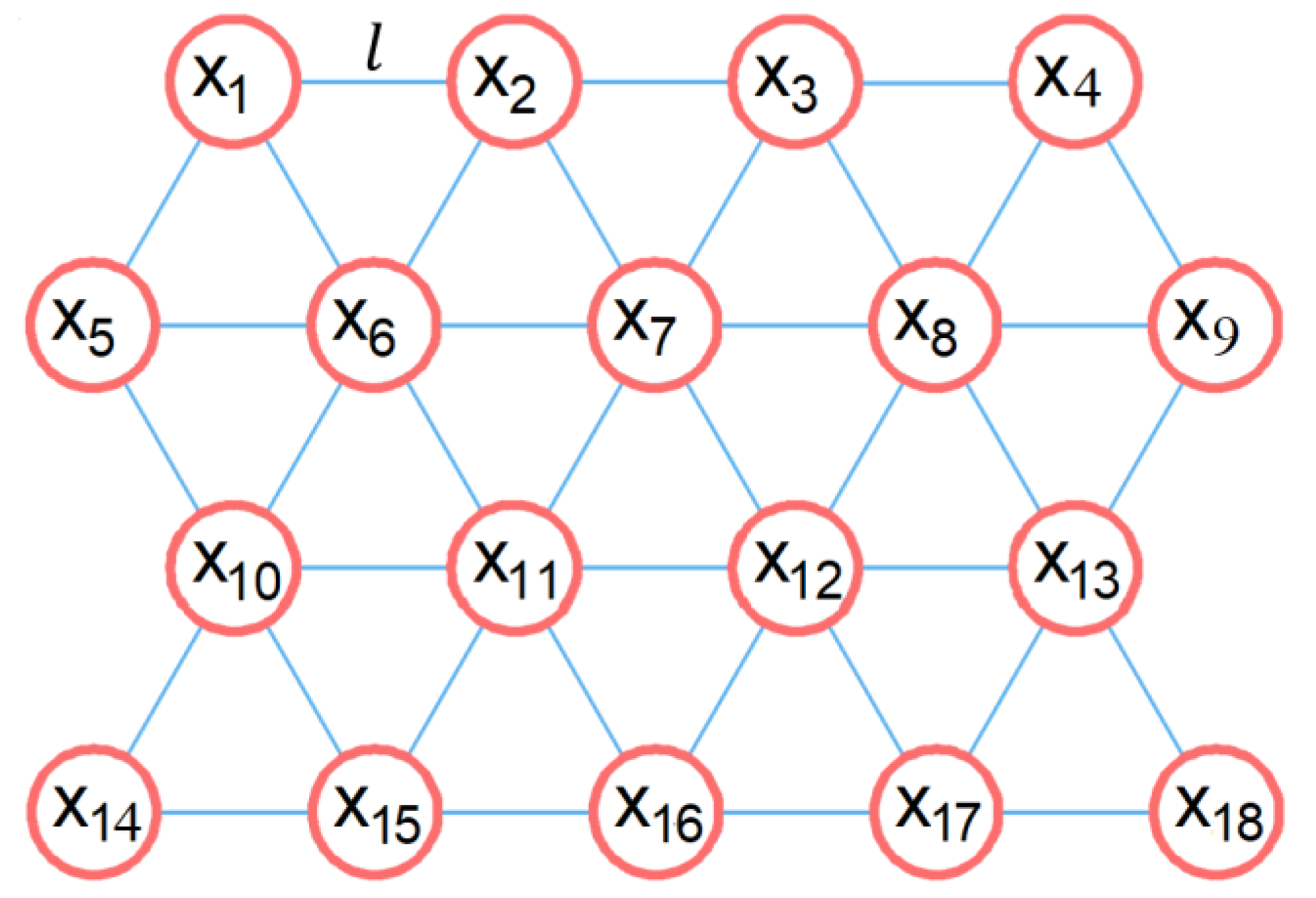
Let the information on level ice thickness and ice concentration be contained in segmentation and coloring of an area of interest in an ice chart. Let us define a graph $G$ in such a part of the ice chart, where each vertex of the graph belongs to a region of certain ice thickness and ice concentration (including zero values of these parameters), and all of the vertices and edges are positioned in places with proper depth.

Let the functions $h$ and $c$ denote the level ice thickness and ice concentration, respectively. Their domain is a continuous water area in the ice chart. In our model, we use discrete $h$ with $E\left(h\right)=\left\{h_1,h_2,\dots , h_p\right\}$, where $p$ = the number of possible ice level thicknesses. Similarly, for function $c$: $E\left(c\right)=\left\{c_1,c_2,\dots ,c_q\right\}$, where $c_1,c_2,\dots ,c_q$—values of ice concentration in the considered area of the ice chart. Now, we can define the functions $h\left(x\right)$ and $c\left(x\right)$ for all $x\in \mathcal{X}$ of the graph $G$.

2.2. Ship Speed Modeling

Another aspect that should be considered when planning routes of ships in ice is ship performance. At first, the routing model should take into account the parameters of a vessel to assess the possibility of operating this vessel in certain ice conditions. Secondly, since ice resists the movement of a vessel, its speed differs in different parts of the route, depending on the ice conditions. Our routing model takes into account the variability of the vessel speed depending on level ice thickness and ice concentration.

Numerous studies on ship performance in level ice are known in the literature, for example [7,14,15,16]. This work does not aim to develop a new model of ship performance in ice. Therefore, to estimate the speed of a vessel’s movement depending on ice conditions, we use a model developed earlier by Kaj Riska. A detailed description of this ship performance model can be found in [7]. Let us consider general provisions of it in relation to ice conditions. Let us divide the procedure of calculating the ship speed $v$ on an edge between two adjacent vertices into two stages:

Step 1. Calculation of the ship speed depending only on the level ice thickness, $v=v\left(h\right)$.

The basis for calculating the ship speed is a comparison of two values: total ice resistance $R$ and net thrust $T_{net}$, namely, the equality (1):

$$T_{net}\left(h\right)=R\left(v,h\right)$$

(1)

The left and the right parts of this equation can be expanded as follows [7]:

$$T_{net}\left(v\right)=\left(1-\frac{1}{3}\frac{v}{v_{ow}}-\frac{2}{3}{\left(\frac{v}{v_{ow}}\right)}^2\right)T_{pull}$$

(2)

$$T_{pull}=K_e{\left(P_s{D}_p\right)}^{\frac{2}{3}}$$

(3)

$$R\left(v,h\right)=C_1\left(h\right)+v{C}_2\left(h\right)$$

(4)

$$\begin{gathered} C_1\left(h\right)={\alpha }_1\frac{1}{2\frac{d}{B}+1}B{L}_{par}h+\left(1+0.021\varphi \right)· \\ \left(\left({\alpha }_{2}B+{\alpha }_3{L}_{bow}\right)h^2+{\alpha }_{4}B{L}_{bow}h\right) \end{gathered}$$

(5)

$$C_2\left(h\right)=\left(1+0.063\varphi \right)\left({\beta }_1{h}^{1.5}+{\beta }_{2}Bh\right)+{\beta }_{3}h\left(1+1.2\frac{d}{B}\right)\frac{B^2}{\sqrt{L}}$$

(6)

All designations found in Formulas (2)–(6) are given in the Nomenclature section at the end of the paper, and values ${\alpha }_1, {\alpha }_2, {\alpha }_3, {\alpha }_4, {\beta }_1,{\beta }_2,{\beta }_3$ required for calculating constants $C_1$ and $C_2$ are presented in

Table 1. Values of constants for ship ice resistance calculations. Reprinted with permission from Ref. [7]. 2009, Elsevier.

Constant	Value	Unit
${\alpha }_1$	$0.23\times {10}^3$	$\mathrm{N}·{\mathrm{m}}^{-3}$
${\alpha }_2$	$4.58\times {10}^3$	$\mathrm{N}·{\mathrm{m}}^{-3}$
${\alpha }_3$	$1.47\times {10}^3$	$\mathrm{N}·{\mathrm{m}}^{-3}$
${\alpha }_4$	$0.29\times {10}^3$	$\mathrm{N}·{\mathrm{m}}^{-3}$
${\beta }_1$	$18.9\times {10}^3$	$\mathrm{N}·\mathrm{s}·{\mathrm{m}}^{-2.5}$
${\beta }_2$	$0.67\times {10}^3$	$\mathrm{N}·\mathrm{s}·{\mathrm{m}}^{-3}$
${\beta }_3$	$1.55\times {10}^3$	$\mathrm{N}·\mathrm{s}·{\mathrm{m}}^{-3.5}$

.

Step 2. Calculation of ship speed depending on both ice thickness and ice concentration,$v=v\left(h,c\right)$.

Considering that $v_{ow}$ is the ship speed in open water and $v_i$ is the ship speed in the level of ice thickness $h$, an estimate of the effect of both ice thickness and ice concentration on the ship speed can be performed using the following formula:

$$v\left(h,c\right)=\{\begin{array}{cc}{v}_{ow}& c\le c_0\hfill \\ \frac{\left(c_1-c\right)v_{ow}+\left(c-c_0\right)v\left(h\right)}{\left(c_1-c_0\right)},& c_0<c<c_1\hfill \\ v\left(h\right)& c\ge c_1\hfill \end{array}$$

(7)

In [7], values of $c_0=7$ and $c_1=9.5$ in terms of ice concentration score are proposed. However, for our case study, we have taken a more conservative $c_0=4,$ assuming that a vessel decreases its velocity at the surrounding ice concentration of 40%. Such a choice was made for illustrating ship velocity variability on the particular ice chart of the case study. The influence of vessel characteristics on values of $c_0$ and $c_1$ in design Formula (7) should be better investigated in the future.

Using parameters of a particular vessel and knowing ice thickness $h\left(x\right)$ and concentration $c\left(x\right)$ in each vertex $x\in \mathcal{X}$, we can evaluate the function $v\left(x\right)=v\left(h\left(x\right),c\left(x\right)\right)$ for that vertex by means of (1)–(7). Now, we have all the necessary parameters to move on to the next paragraph, which describes the routing model we developed and the methods and algorithms for its implementation.

2.3. Optimization Methods and Algorithm

A route is an ordered sequence of adjacent vertices of a graph, and there are no cycles in this sequence. Let vertices $x_S\in \mathcal{X}$ and $x_F\in \mathcal{X}$ be the start and finish points of the route to be found, respectively: $T=\left\{x_S, \dots ,x_F\right\}$, $T\in \mathcal{K}$. Here, $\mathcal{K}$ is the set of all possible acyclic routes from the node $x_S$ to the node $x_F$ on the graph $G\left(\mathcal{X},\mathcal{U}\right)$.

Let us consider objective functions for our optimization model. Let the function $f_1$ take on the value of the length of a route $T$ from the set $\mathcal{K}$:

$$f_1\left(T\right)=\left(\left|T\right|-1\right)·l$$

(8)

Here, $l$ is the length of the graph edge. Optimal routes with respect to the first objective function satisfy the following criterion:

$$T_k^1:f_1\left( T_{k1}^1\right)=\underset{ T\in \mathcal{K}}{\min }{f}_1\left(T\right)$$

(9)

where $T_{k1}^1$ is a route from the set of equally optimal routes by the criterion (9).

Let functions $f_2$ and $f_3$ take the maximum possible value of level ice thickness and ice concentration on the route $T\in \mathcal{K}$, respectively:

$$f_2\left(T\right)=\underset{x\in T}{\max }\left(h\left(x\right)\right)$$

(10)

$$f_3\left(T\right)=\underset{x\in T}{\max }\left(c\left(x\right)\right)$$

(11)

Then, we consider the following conditions (12) and (13) for objective functions $f_2$ and $f_3$, which provide us with sets $T_{k_2}^2$ and $T_{k_3}^3$ of routes:

$$T_{k_2}^2:f_2\left( T_{k_2}^2\right)\le h_{thr}$$

(12)

$$T_{k_3}^3:f_3\left( T_{k_3}^3\right)\le c_{thr}$$

(13)

Here, $h_{thr}$ and $c_{thr}$ are the threshold values for functions $h$ and $c$, respectively. This way, the objective functions $f_2$ and $f_3$ define acceptable risks along the route.

Using the fact that $h$ and $c$ are discrete functions, we can consider all the possible combinations of pairs $\left(h_{thr},c_{thr}\right)$ and solve the problem (9) with respect to (12) and (13) for each of the pair.

Sometimes, the length of the route is not the most important parameter for choosing a favorable route for a vessel. Hence, we introduce an additional function $f_4$, which takes on the value of the ship travel time (11) on the route.

$$f_4\left(T\right)=l{\displaystyle \sum }_{x\in T}\frac{1}{v\left(x\right)}$$

(14)

The authors use the idea of a wave algorithm for the following optimization method. The wave algorithm is based on sequential indexing of adjacent graph vertices. The initial vertex is $x_S\in \mathcal{X}$. Wave propagation across the graph and indexing of vertices is performed until the vertex $x_F\in \mathcal{X}$ is reached. Then, in reverse propagation, the minimum length route is found.

The authors of this paper have developed an additional algorithm that expands the capabilities of the wave method. The concept of the extended wave algorithm (EWA) allows us to find the entire set of the equally shortest routes from the start $x_S$ to the finish $x_F$ on graph $G$ by means of recursive function using the indices assigned for the vertices.

Thus, the objective functions and the optimization method for the problem of finding the optimal route of the vessel in ice conditions has been determined. It is clear that without knowing which of the functions is the most preferable, it is impossible to find the only optimal solution for the problem. Nevertheless, we can find sets of Pareto-optimal solutions for the considered combination of objective functions. We say that the route is Pareto-optimal if none of its legs can be changed without worsening at least one of the considered objective functions for this route [17].

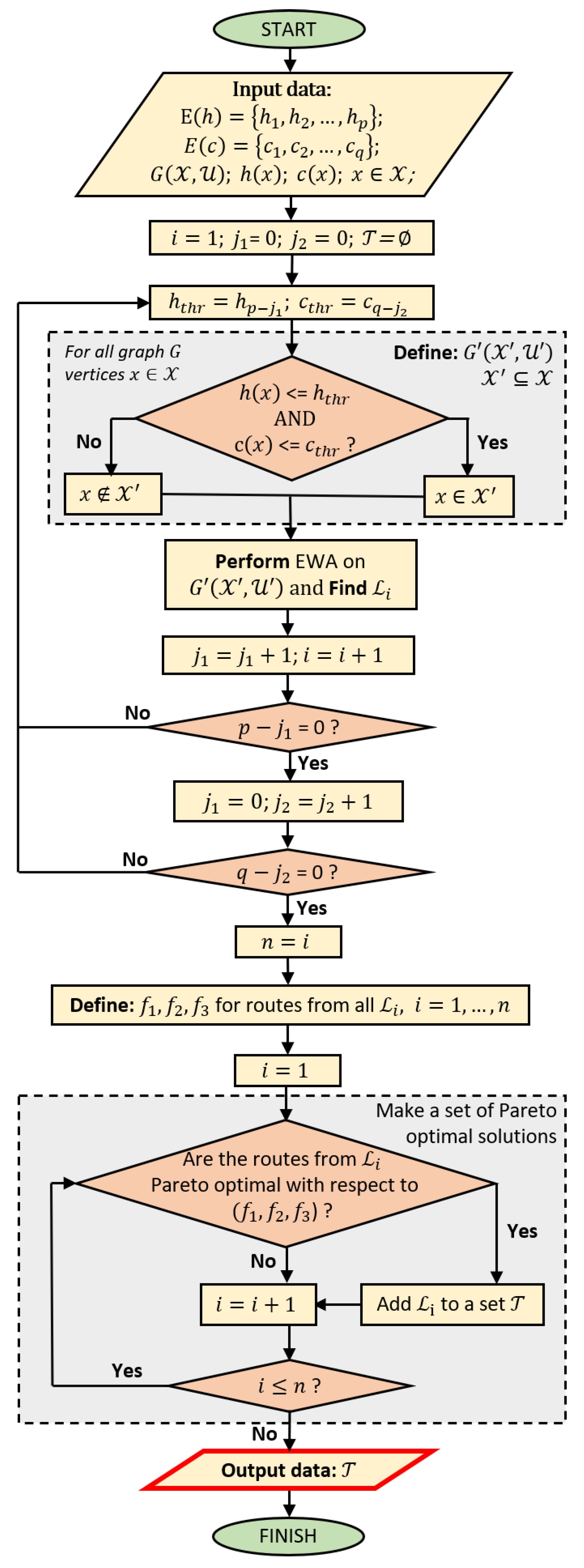
Let us introduce Algorithm 1 for finding a complete set of Pareto-optimal solutions $\mathcal{T}$ for objective functions $\left(f_1,f_2,f_3\right)$. A block diagram for the algorithm is presented in Figure 2. The developed algorithm is based on checking all pairs $\left(f_2,f_3\right)$. For each of these pairs, we form a new graph $G^{\prime }\left({\mathcal{X}}^{\prime },{\mathcal{U}}^{\prime }\right)$, employ the EWA with a recursive function in the backpropagation search, and find the set ${ℒ}_i$ of equally optimal solutions of (9) on$G^{\prime }\left({\mathcal{X}}^{\prime },{\mathcal{U}}^{\prime }\right)$. Not every ${ℒ}_i$ found for a particular pair $\left(h_{thr},c_{thr}\right)$ belongs to the set $\mathcal{T}$ of Pareto-optimal routes. An additional examination of routes’ non-deterioration in the sense of their objective values $\left(f_1,f_2,f_3\right)$ when shifting from ${ℒ}_i$ is required.

In a general case, the cardinality of set ${ℒ}_i$ is quite big. We can consider the fourth objective function (14) and find optimal routes in regard to $\mathcal{T}$, which will provide us with the solution of the problem with lexicographically ordered criteria:

$$lex\underset{T\in \mathcal{K}}{\min }\left(\left(f_1,f_2,f_3\right),f_4\right)$$

(15)

3. Application

In the previous section, a theoretical description of the ice routing model proposed by the authors was given. In this section, the authors describe its practical application. The input parameters of the model are the ice chart image, the initial and final coordinates of the planning route, and the characteristics of the vessel.

One of the important components for practical application of the model is the visualization of the simulation results in a convenient format. In our model, the output data are a set of Pareto-optimal routes for the multi-objective problem and descriptive characteristics of these routes. The resulting sequence of waypoints are presented graphically on the ice chart.

3.1. Interpretation of Ice Chart

In order to set the graph and to apply the developed optimization algorithm, it is necessary to extract information on ice conditions from an ice chart. For the Northern Baltic Sea, ice charts [18] and ice conditions prognoses [19] are issued on a regular basis. We used the ice charts of the Gulf of Finland issued by the Finnish Meteorological Institute (FMI) [18]. In such charts, the information on ice concentration is given by color, while ranges of ice thickness are assigned to color regions. Thus, firstly, we need to process and retrieve the information from the image by means of contouring. We performed recognition using the automatic software developed by us. For example, Figure 3a shows contouring of the new ice (light pink) areas. Figure 3b shows the graph $G\left(\mathcal{X},\mathcal{U}\right)$ positioned on the contoured ice chart. In

Table 2. Legend for color areas of the images in Figure 3a,b and Figure 4a–f; $v$ is the design speed for the ship considered in the case study.

Color	Ice Conditions	$\mathit{c}$	$\mathit{h}$, m	$\mathit{v}$, m/s
	Open water	1	0	7
	Open ice	5	0.2	6.736
	Close ice	7.5	0.2	6.077
	Very close ice	9	0.2	5.682
	Consolidated ice	10	0.2	5.418
	New ice	8.5	0.025	6.818
	Thin level ice	9.5	0.1	6.402
	Fast ice	10	0.325	4.475

, the color legend for ice types in Figure 3a,b and Figure 4a–f is provided.

3.2. Case Study

This section considers a computational example of applying the developed method in the case of the Eastern Gulf of Finland of the Baltic Sea. The Baltic Sea is one of the busiest waterways in the world and is partly covered with ice every winter [1]. In addition, as it has been already noted, there are relatively a lot of reliable meteorological data sources for the Baltic Sea area, including on ice conditions. These are the reasons why the Baltic Sea area is excellent for modeling the optimal routes of a vessel in ice. The case study for the ice chart dated 11 March 2021 will be considered in this work [18].

Let us define graph $G(\mathcal{X},\mathcal{U}$) with triangular cells to the entire area of the ice map (Figure 3b). The edge size of the graph $G$ is $l=6.06 \mathrm{km}$, and the cardinality of the sets of vertices and edges of the graph is $\left|\mathcal{X}\right|=513$ and $\left|\mathcal{U}\right|=1419$, respectively.

Ice thickness and ice concentration in ice maps are usually given by intervals. Therefore, when determining the domains of functions $h\left(x\right)$ and $c\left(x\right)$, we calculate the average values of such intervals (columns “c” and “h” in Table 2). In our computational example, the domains of the mentioned functions are the following: $E\left(c\right)=\left\{1;5;7.5;8.5;9;9.5;10\right\}$ and $E\left(h\right)=\left\{0;0.025;0.1;0.2;0.325\right\}$. Thus, we assign ice thickness and ice concentration for each color zone of the image, obtaining values of these functions for each node $x_i\in \mathcal{X}$ of the graph $G$, $i=1, 2, \dots , 513$ presented in Figure 3b.

Let us perform Algorithm 1 (Figure 2) for solving problems (9)–(13) and find $\left|E\left(c\right)\right|·\left|E\left(h\right)\right|=35$sets ${ℒ}_i$. Due to peculiarities of the ice chart, 15 of them turned out to be empty; the information on the others is provided in

Table 3. Values of $f_1$ at $\left(h_{thr},c_{thr}\right)$ for problems (9)–(13) applied for the graph in Figure 3b; Pareto-optimal solutions are shaded.

${\mathit{h}}_{\mathit{t}\mathit{h}\mathit{r}}$$\backslash {\mathit{c}}_{\mathit{t}\mathit{h}\mathit{r}}$	1	5	7.5	8.5	9	9.5	10
0	-	-	-	-	-	-	-
0.025	-	-	-	$25l$	$25l$	$25l$	$25l$
0.1	-	-	-	$25l$	$25l$	$24l$	$24l$
0.2	-	$33l$	$24l$	$21l$	$21l$	$19l$	$19l$
0.325	-	$33l$	$24l$	$21l$	$21l$	$19l$	$19l$

. Eventually, only six sets of ${ℒ}_i$ make up the Pareto-front; corresponding cells in Table 3 are shaded with grey. Here, we enumerate them as follows: $\mathcal{T}=\left\{{ℒ}_1,{ℒ}_2,{ℒ}_3,{ℒ}_4,{ℒ}_5,{ℒ}_6\right\}$. The values of the objective functions for routes from ${ℒ}_i\in \mathcal{T}$ along with $\left|{ℒ}_i\right|$ are presented in

Table 4. Characteristics of Pareto-optimal routes from the set ${ℒ}_i$ as illustrated in Figure 4a–f.

	${\mathit{ℒ}}_1$	${\mathit{ℒ}}_2$	${\mathit{ℒ}}_3$	${\mathit{ℒ}}_4$	${\mathit{ℒ}}_5$	${\mathit{ℒ}}_6$
$\left|{ℒ}_i\right|$	2430	21	2645	3	2550	50,388
$f_1\left(T\right)$	$33l$	$24l$	$25l$	$21l$	$24l$	$19l$
$f_2\left(T\right)$	0.2	0.2	0.025	0.2	0.1	0.2
$f_3\left(T\right)$	5	7.5	8.5	8.5	9.5	9.5
$f_1\left(T\right),$ km	200	145.4	151.5	127.3	145.4	115.1
$f_4\left(T\in {ℒ}_i^{*}\right)$, h	8	6.19	6.08	5.24	5.93	5.0

. Figure 4 shows the ice chart with all the Pareto-optimal routes, 58,037 in total.

It is difficult for a user to work with such a large set of optimal solutions. Let us reduce the number of solutions of interest by applying an additional objective function $f_4$ (14) that optimizes solutions in terms of the total travel time. For this, we have taken the parameters (

Table 5. Ship parameters.

Parameter	Parameter Description	Value	Unit
$T$	Ship draught	9.03	m
$B$	Ship maximum breadth	24.6	m
$L_{par}$	Length of the ship parallel midbody	120	m
$\varphi$	Bow angle	0.96	rad
$L_{bow}$	length of the ship bow	19	m
L	Ship length	157	m
$v_{ow}$	Open water speed	7	m/s
$P_s$	Propulsion power	7860	kW
$D_p$	Propeller diameter	3.8	m

) of a random ship. Using these parameters, Formulas (2)–(7) of the ship performance model, thresholds of ice concentration $c_0$ and $c_1$ for (7), and coefficients listed in Table 1, we can find velocity $v\left(x\right)$ of a ship in any node $x$ of the graph $G$ with known $\left(h\left(x\right),c\left(x\right)\right)$. Here, we have taken $c_0$ and $c_1$ as 4 and 10, respectively.

As the final recommendation for a navigator, we chose those routes from each particular set ${ℒ}_i$ $i=1,2,\dots ,6$, which provide minimal value of function (14). As a result, we obtained six subsets of routes ${ℒ}_i^{*}$, ${ℒ}_i^{*}\subseteq {ℒ}_i$. This led to a decrease in the number of the routes of interest by ~90%. The routes from set ${ℒ}_i^{*}$ are shown in green in Figure 4. Figure 5 presents two plots of vessel speed in time for routes shown with green in Figure 4e,f. To suggest a single route on the basis of ${ℒ}_i^{*}$, heuristic algorithms can be applied.

The practical application of the developed model is based on information that can be derived from an ice chart. In such charts, the tracing and sail/keel parameters of ice ridges are usually not specified. Because of this, ice ridges have not been taken into consideration at the moment. However, with the improvement of data availability on ridges location and their parameters, ice ridges can be included in the model.

4. Discussion

The method developed in this paper as well as the case study are intended for use in freezing parts of the Baltic Sea. For this region, ice conditions are usually not very severe, which allows for independent navigation by the wide range of ships to be practiced. Moreover, detailed ice charts are issued on a regular daily basis for the Baltic, and depths in the region are well known, which allows us to confidently set a transportation graph with rather short edges.

However, for the Arctic, the situation is different. Thick and close ice in the region in the winter season as well as uncertain conditions due to the lack of detailed and relevant information hamper the development of models for independent routing in this region. Earlier, some of the graph-based transportation models were suggested for Arctic conditions [20,21,22,23]. There, mainly graphs with long-distance edges, representing alternatives between a number of routing points had been used. For Arctic conditions, a special ship performance model should be developed, unlike Riska’s model. For instance, a cargo vessel speed reduction model depending on Arctic ice conditions is proposed in [21]. As route optimization algorithms Dijkstra [21] and A* [22,23] was applied. We should note that the optimization made by these algorithms is single-criteria.

5. Conclusions

In this work, the multi-objective problem of ice navigation routing with risk objective functions in the form of maximum ice thickness and concentration on the route is stated and solved. The problem is stated in the discrete form by means of the graph. The stepwise algorithm on this graph was proposed, which allows us to find sets of routes with minimal length in specific risk conditions. From these sets, the Pareto-optimal set for the three-objective length-risk problem is made. For modeling ship performance in ice conditions, Riska’s model was employed. This ship performance model allows us to find the most time efficient route from the previously found Pareto-optimal set.

The case study of multi-objective route optimization in the eastern area of the Gulf of Finland based on the ice chart information for 11 March 2021 is performed. In this case study, the route in ice-infested waters was optimized for a hypothetic vessel; the result was obtained both in the form of sets of possible routes and in the form of the Pareto-front in the objective space. On the found set of routes, the travel time was optimized by means of a ship performance model.

References

1. Vihma, T.; Haapala, J. Geophysics of sea ice in the Baltic Sea: A review. Prog. Oceanogr. 2009, 80, 129–148. [Google Scholar] [CrossRef]
2. Montewka, J.; Goerlandt, F.; Kujala, P.; Lensu, M. Towards probabilistic models for the prediction of a ship performance in dynamic ice. Cold Reg. Sci. Technol. 2015, 112, 14–28. [Google Scholar] [CrossRef]
3. Valdez Banda, O.A.; Goerlandt, F.; Montewka, J.; Kujala, P. A risk analysis of winter navigation in Finnish sea areas. Accid. Anal. Prev. 2015, 79, 100–116. [Google Scholar] [CrossRef] [PubMed]
4. Zis, T.P.V.; Psaraftis, H.N.; Ding, L. Ship weather routing: A taxonomy and survey. J. Ocean Eng. 2020, 213, 107697. [Google Scholar] [CrossRef]
5. Riska, K.; Patey, M.; Kishi, S.; Kamesaki, K. Influence of ice conditions on ship transit times in ice. In Proceedings of the 16th POAC Conference, Ottawa, ON, Canada, 12–17 August 2001; Volume II, pp. 729–746. [Google Scholar]
6. Frederking, R. A model for ship routing in ice. In Proceedings of the 17th POAC Conference, Trondheim, Norway, 16–19 June 2003; Volume II, pp. 467–476. [Google Scholar]
7. Kotovirta, V.; Jalonen, R.; Axell, L.; Riska, K.; Berglund, R. A system for route optimization for ice-covered waters. Cold Reg. Sci. Technol. 2009, 55, 52–62. [Google Scholar] [CrossRef]
8. Guinness, R.E.; Saarimäki, J.; Ruotsalainen, L.; Kuusniemi, H.; Goerlandt, F.; Montewka, J.; Berglund, R.; Kotovirta, V. A method for ice-aware maritime route optimization. In Proceedings of the 2014 IEEE/ION Position, Location and Navigation Symposium—PLANS 2014, Monterey, CA, USA, 5–8 May 2014; pp. 1371–1378. [Google Scholar] [CrossRef]
9. Hinnenthal, J.; Clauss, G. Robust Pareto-optimum routing of ships utilising deterministic and ensemble weather forecasts. Ships Offshore Struct. 2010, 5, 105–114. [Google Scholar] [CrossRef]
10. Deco, A.; Frangopol, D.M. Risk-informed optimal routing of ships considering different damage scenarios and operational conditions. J. Reliab. Eng. Syst. Saf. 2013, 119, 126–140. [Google Scholar] [CrossRef]
11. Zvyagin, P.; Voitkunskaia, A. Model of Transit Transport in Arctic Based on Graph Algorithms. In Proceedings of the 35th OMAE Conference, Busan, Korea, 18–24 June 2016; p. 6. [Google Scholar] [CrossRef]
12. Wang, H.; Mao, W.; Eriksson, L. A Three-Dimensional Dijkstra’s algorithm for multi-objective ship voyage optimization. J. Ocean. Eng. 2019, 186, 106–131. [Google Scholar] [CrossRef]
13. Zvyagina, T.; Zvyagin, P. A model of multi-objective route optimization for a vessel in drifting ice. Reliab. Eng. Syst. Saf. 2022, 218, 108–147. [Google Scholar] [CrossRef]
14. Lindqvist, G. A straightforward method for calculation of ice resistance of ships. In Proceedings of the 10th POAC Conference, Luleå, Sweden, 12–16 June 1989; pp. 722–735. [Google Scholar]
15. Hu, J.; Zhou, L. Further study on level ice resistance and channel resistance for an icebreaking vessel. Int. J. Nav. Archit. Ocean. Eng. 2016, 8, 169–176. [Google Scholar] [CrossRef] [Green Version]
16. Milaković, A.S.; Li, F.; von Bock und Polach, R.U.F.; Ehlers, S. Equivalent ice thickness in ship ice transit simulations: Overview of existing definitions and proposition of an improved one. Ship Technol. Res. 2020, 67, 84–100. [Google Scholar] [CrossRef]
17. Ehrgott, M. Multicriteria Optimization, 2nd ed.; Springer: Berlin/Heidelberg, Germany, 2005; 323p. [Google Scholar] [CrossRef] [Green Version]
18. Ice Charts for Northern Baltic. Available online: https://en.ilmatieteenlaitos.fi/ice-conditions (accessed on 11 March 2021).
19. Baltic Sea Ice Forecast. Available online: https://ice.fmi.fi/data/baltic-sea/sea-ice-forecast/ (accessed on 14 September 2020).
20. Choi, K.S.; Nam, J.H.; Park, Y.J.; Ha, J.S.; Jeong, S.Y. Northern sea route transit analysis for large cargo vessels. In Proceedings of the 25th International Symposium on Okhotsk Sea & Sea Ice, Mombetsu, Japan, 21–26 February 2010; pp. 194–200. [Google Scholar]
21. Nam, J.H.; Park, I.; Jin Lee, H.; Ok Kwon, M.; Choi, K.; Seo, Y.K. Simulation of optimal arctic routes using a numerical sea ice model based on an ice-coupled ocean circulation method. Int. J. Nav. Archit. Ocean. Eng. 2013, 5, 210–226. [Google Scholar] [CrossRef] [Green Version]
22. Choi, M.; Chung, H.; Yamaguchi, H.; Nagakawa, K. Arctic sea route path planning based on an uncertain ice prediction model. Cold Reg. Sci. Technol. 2015, 109, 61–69. [Google Scholar] [CrossRef]
23. Zhang, M.; Zhang, D.; Fu, S.; Zhang, C. A method for planning Arctic sea routes under multi-constraint conditions. In Proceedings of the 24th POAC Conference, Busan, Korea, 10–16 June 2017. [Google Scholar]
Figure 1. Graph with triangular cells.
Jmse 10 00862 g001
Figure 2. Block diagram of Algorithm 1.
Jmse 10 00862 g002
Figure 3. Input data preparation: (a) segmentation of the ice chart; (b) defining graph G ( X , U ) on the area.
Jmse 10 00862 g003
Figure 4. Graphical representation of all i Pareto-optimal routes for the set of conditions given in Table 3 with respect to objective functions f 1 , f 2 , and f 3 . Characteristics of these routes are provided in Table 4. Optimal routes with respect to objective function f 4 (travel time) are given in green.
Jmse 10 00862 g004
Figure 5. Ship speed in time for routes shown with green in Figure 4e (red line) and Figure 4f (blue line).
Jmse 10 00862 g005