Multi-Objective Weather Routing Algorithm for Ships: The Perspective of Shipping Company’s Navigation Strategy

Abstract

Ship weather routing has always been an important issue in the research field of navigation, and many scholars have been devoted to this research for a long time. To study the route strategies of different shipping companies, this paper proposes an improved multi-objective ant colony optimization (IMACO) algorithm based on the Technique for Order Preference by Similarity to Ideal Solution (TOPSIS). It can comprehensively consider ship navigation risk and fuel consumption cost under complex sea conditions. First, the grid method is used to model the marine environment. Then, we calculate the fuel consumption and the ship navigation risk of each grid and use the TOPSIS method to evaluate these two indicators for each grid. The results show that due to the different strictness of navigation management requirements of different companies, different routes are selected in the same sea area at the same time. Compared with the single-objective ant colony optimization (SACO) algorithm, the algorithm proposed in this paper can more comprehensively and effectively solve the problem of route strategy selection of shipping companies, which has great practical significance for ship operations management.

1. Introduction

Waterway transportation plays an important role in global trade. According to statistics, more than 80% of global trade is realized by shipping [1]. To promote its sustainable development, it is necessary to reduce the fuel consumption of ships, decrease navigation risks, and shorten navigation time [2]. Historically, fuel costs were small compared with the fixed cost of the vessel, its crewing and management, while today it accounts for more than 50% of the cost [3]. This indicates that even a partial reduction in fuel consumption will save shipping companies’ substantial economic cost. At the same time, reducing the fuel consumption of ships is an effective way to control the emission of pollution sources at the source. It is in line with the growing concern for environmental protection and sustainable development in the international shipping field, such as the emission control area (ECA) and the IMO’s upcoming Energy Efficiency Existing Ship Index (EEXI).

However, the marine meteorological environment has the characteristics of complexity and variability. Severe weather conditions threaten the navigation safety of ships, and shipwrecks are common. Such conditions can not only cause damage to ships but also seriously threaten the lives of crew members [2]. At present, the research on ship route planning concerning complex sea conditions has become a hot spot in the international maritime field. How to make ships navigate more safely and efficiently in such conditions is of great significance to the development of the maritime industry.

Current research on ship weather routing can be divided into global path planning based on maritime environmental information and local path planning. Global path planning refers to the static obstacle layout in the environment, which is obtained based on the given environmental information, and then a suitable path from the starting point to the global target is sought with a path planning search algorithm [4]. Park et al. [5] proposed a new approach based on A* algorithm to solve the weather routing problem. It reduced the fuel consumption by 3.2 and 2.1% and could be applied to the general weather routing cases. Mannarini et al. [6] proposed an automated ship routing decision support system. The system used a modified Dijkstra algorithm for a directed graph to select the best route. Zhou et al. [7] proposed a modified genetic algorithm to find a safe and time-saving route for ships. He introduced the deletion and insertion operator, the modified mutation operator, and the smoothing operator to make the algorithm more suitable for route planning. According to the above literature, algorithms of global path planning mainly include the A* algorithm, the Dijkstra algorithm, and the genetic algorithm. They are mainly used to solve the optimization problem of static route planning. As for local path planning, it is more suitable for dynamic path optimization. Its methods include the isochrone method and dynamic programming. The isochrones method was originally proposed by Hanssen et al. [8] to optimize routing in stationary weather conditions. The modified isochrone method was extended by Hagiwara [9]. He used the method of definite integrals to minimize either time, fuel, or cost. Szlapczynska et al. [10] provided an adaptation proposal of the isochrone method with area partitioning. It proved that the route selected by the adopted method would not cross land. Later scholars such as Roh [11] proposed an improved isochrone method to determine economical shipping routes based on real-time marine information and the estimation of fuel consumption. Dynamic programming implements multi-stage decisions based on Bellman’s principle of optimality [12], so that each part is optimal to achieve the overall optimality. Zoppoli [13] solved the problem of determining minimum-time ship routes by dynamic programming. He described it as a discrete decision process in stochastic conditions. Barber et al. [14] presented a parallel dynamic programming algorithm in a highly computer intensive combinatorial problem. It could be used in ship voyage management. Shao et al. [15] proposed a forward three-dimensional dynamic programming (3DDP) method. The method includes ship power settings and heading control changes and aims to minimize fuel consumption. Skoglund et al. [16] proposed a new dynamic programming algorithm which is adapted for use with ensemble weather forecasts. By adding robustness as an additional objective, it was able to compute Pareto optimal solutions to a multi-objective routing problem. However, local path planning has poor overall route planning performance since it can only obtain local information from ship equipment and cannot obtain global environmental information in advance. Therefore, in this study, we use the IMACO algorithm to study the route selection of different shipping companies in the global environment.

Optimization objectives in route planning are also the long-term research object of various scholars. Prpić-Oršić et al. [17] thought the influence of various parameters such as ship initial speed (full ahead and lower engine loads), loading condition, heading angle and weather conditions on ship fuel consumption and CO₂ emission would affect the ship’s route selection. They calculated the weather routing of ships across the Atlantic Ocean, taking into account the ships’ CO₂ emissions and speed losses. Kuhlemann et al. [18] presented a genetic algorithm to minimize the fuel consumption of a ship. The results showed that it could save more than 10% of the fuel consumption when the sea condition was taken into account. Taking a T300k VLCC oil tanker as the research object, Du et al. [19] established a ship route estimation model with minimum fuel consumption, CO₂ emissions and shortest ETA as the objective function, which considers the weather conditions and constraints of the main engine rated power and safety comprehensively. Lindstad et al. [3] developed a model to assess profit, cost and emissions by varying speed as a function of sea conditions and the freight market. The authors focused on different wave heights and combined different market conditions to design a speed that minimized cost or profit. It can be seen that the optimization objective of the shipping route mainly includes minimum sailing time, minimum fuel consumption, minimum emission, or the shortest sailing distance. Unfortunately, many of these studies consider only a single optimization objective [17,18,20,21,22], and although multiple objectives are considered, they do not consider it as a simultaneous planning objective but perform repetitive optimizations on these objectives separately [2,3,19].

Therefore, to counteract the aforementioned problems, a multi-objective weather routing algorithm for ships is proposed in this paper. The paper makes contributions mainly in the following three aspects:

• Proposal of a multi-objective ACO algorithm

Considering the shortcomings of multi-objective planning in voyage optimization, this paper proposes a multi-objective ACO algorithm that takes into account the sea conditions of wind and waves. It aims to achieve safety and reduce fuel consumption cost. This paper considers that ships have to overcome the impact of wind and waves on their operational performance. Besides, when choosing a route, shipping companies need to meet vessel schedule reliability and profit maximization.

2.

Proposal of the concept of “Operational Obstacle”

We propose the concept of the operational obstacle. It can visualize ship navigation risk and fuel consumption cost of shipping companies in the grid environment in the form of obstacles.

3.

Analysis from the perspective of the shipping company’s route strategy

The main body of current research on route planning is limited to studying optimization objectives under different route selections from the perspective of ships. However, in the maritime transportation market, due to the different management levels and risk preferences of different shipping companies, only considering the shortest route and optimal goals from the perspective of the route cannot meet the operating levels of different companies. Therefore, this paper is the first to study weather routing from the perspective of shipping companies. Taking into account the management level and preferences of different shipping companies, and using the proposed multi-objective planning ant colony algorithm, it will guide the shipping companies to provide the route selection that conforms to their own characteristics in the practice of cargo transportation.

The rest of this paper is organized as follows: Section 2 establishes an environmental grid model, analyzes the movement of ships under wind and waves and the calculation of safety and fuel consumption cost indicators, and introduces the improved ant colony algorithm for multi-objective planning, which is combined with TOPSIS method; Section 3 conducts simulation experiments to analyze the route strategies of different shipping companies and verifies the feasibility of the algorithm; Section 4 concludes this paper.

2. Materials and Methods

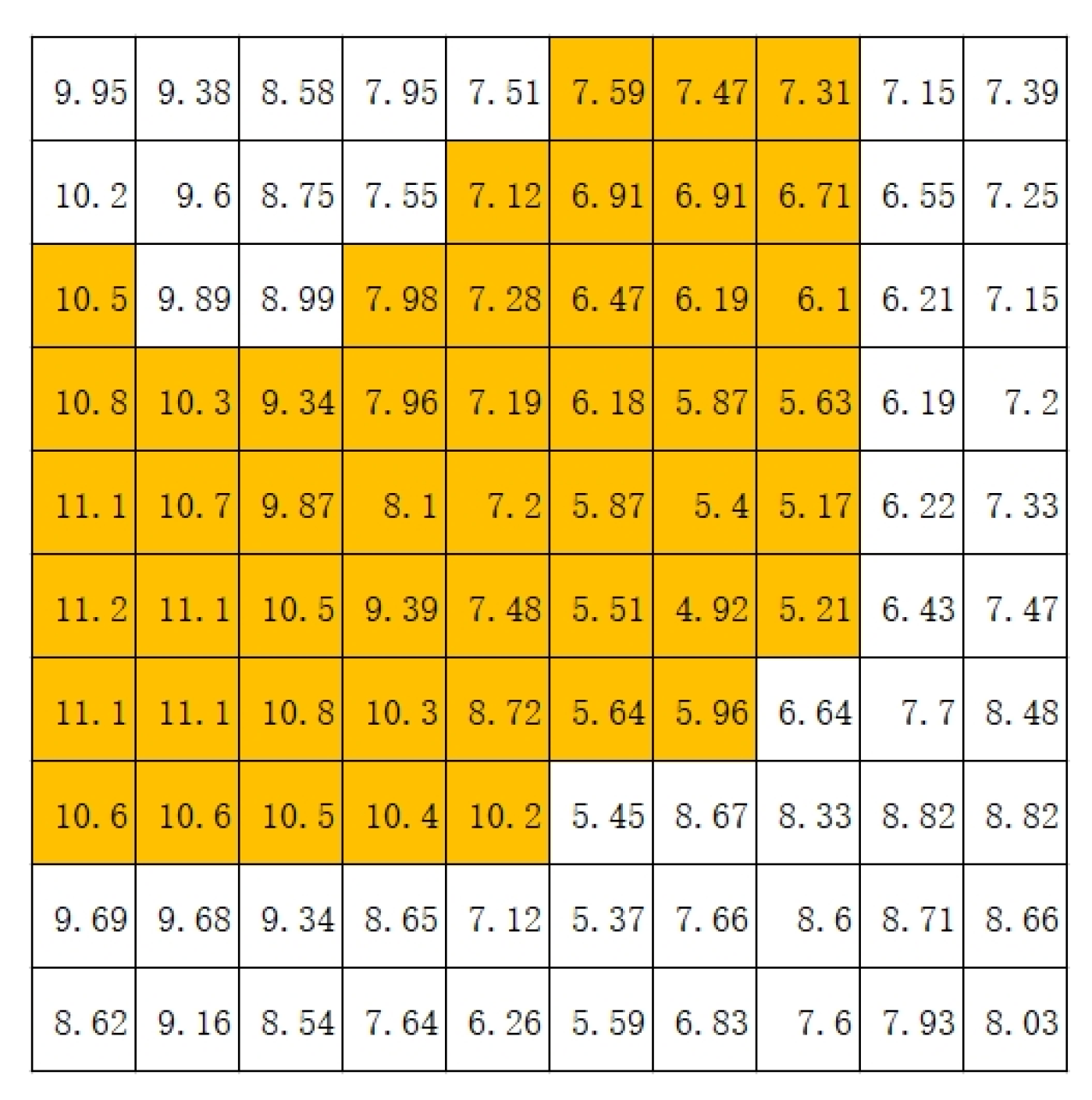
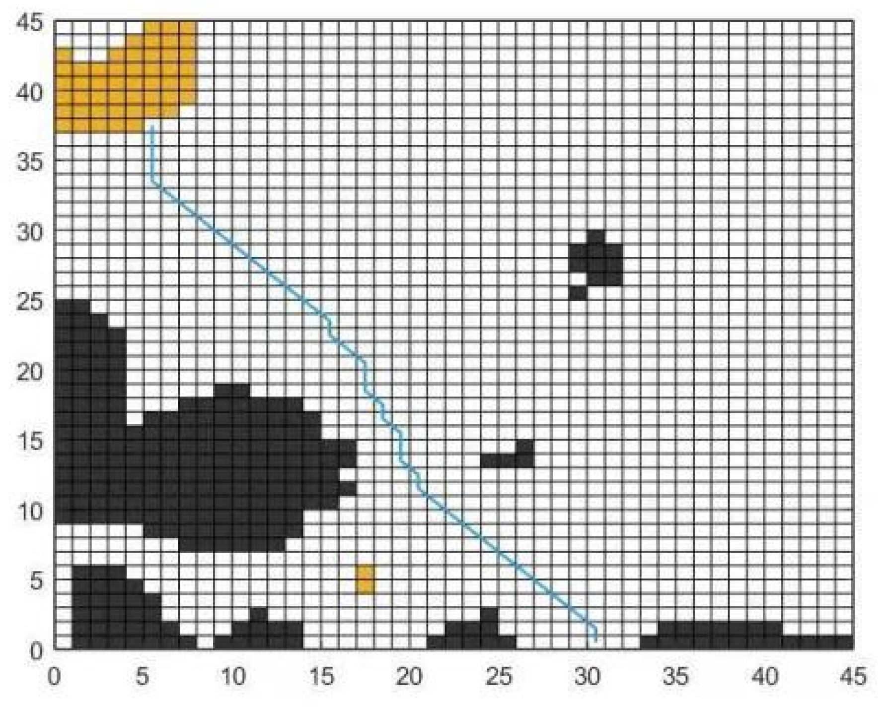
2.1. Grid Method Environment Modeling

In route planning issues, grid maps are often used to establish a static simulation environment. Howden [23] first proposed the grid method, the basic principle of which is to divide the robot working environment into countless small grid cells with binary information. The specification of each grid is determined by the step size of the robot, i.e., one step size represents one grid unit. During grid division, when either the obstacle grid or the non-obstruction grid is not full, fill it up and calculate it as one grid. The grid method represents the infeasible area and the free area with a binary matrix, in which 1 represents the obstacle grid, 0 represents the free grid.

In this paper, the grid method is used to divide the marine environment according to the resolution of $0.5°\times 0.5°$. First, we use python to obtain meteorological data from the European Centre for Medium-Range Weather Forecasts, and download the raster data of the global wind direction, wind speed, wave direction and wave height in the specified area at the specified time. The procedure is in Appendix A. Then, we use the serial number method to identify the grids, and mark them as serial numbers $1,2,3\dots ,n$ in the order from left to right and top to bottom, where each serial number represents a grid.

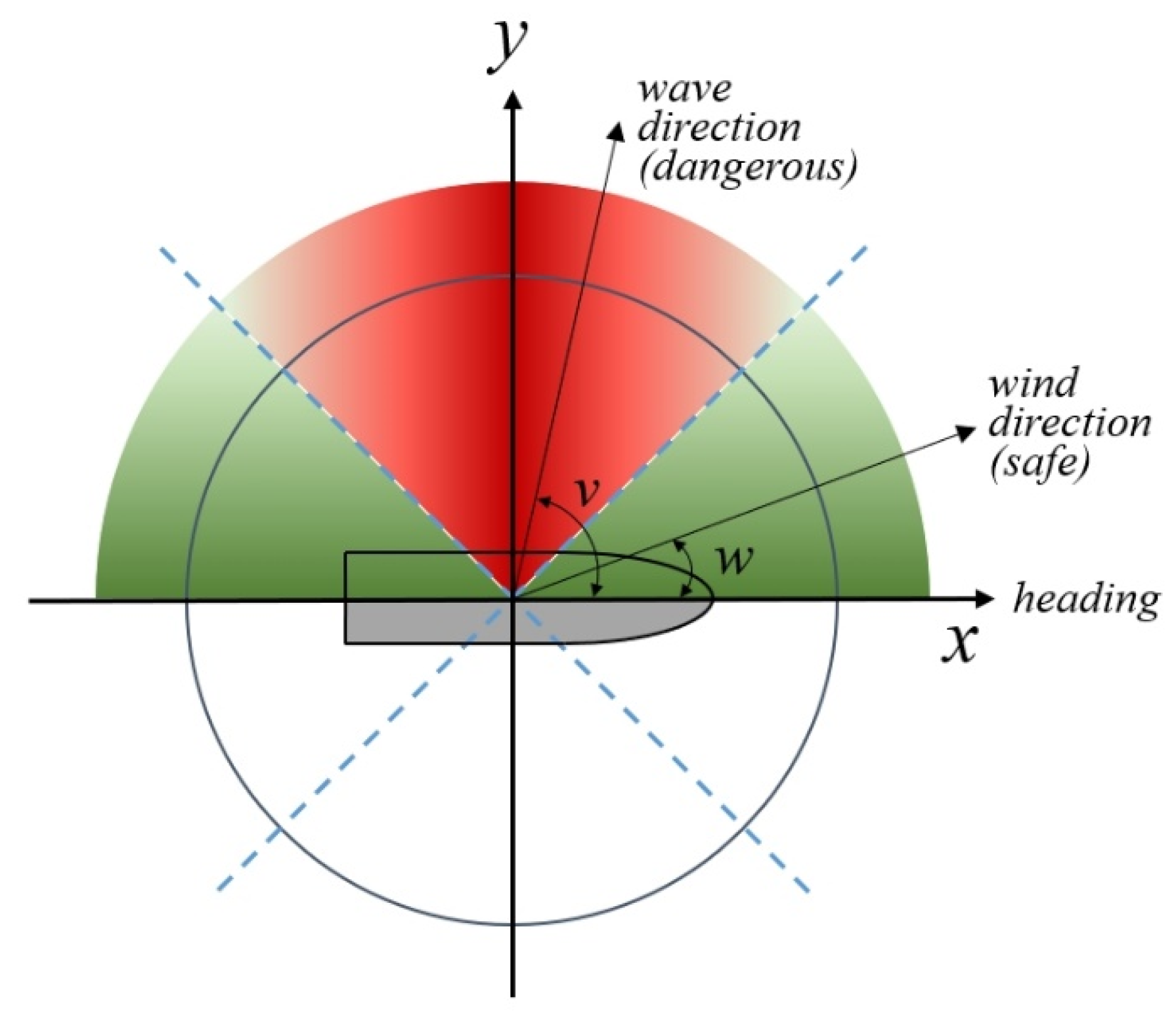
2.2. Impact of Wind and Waves on Ship Stall

In the process of sailing at sea, the speed of the ship in still water is called the speed of the ship, that is, the speed of the ship relative to the sea. However, under the influence of environmental factors such as wind, waves and currents, the ship often cannot reach the set speed. The speed loss will affect the level of fuel consumption of ships. Meanwhile, it will also affect the simulation results of ship weather routing. Therefore, ship stall is an important factor that must be considered in ship weather routing. The actual speed of the ship after considering the influence of the ship’s stall, that is, the sailing speed of the ship relative to the seabed, is called sailing speed. The stall model with waves as the stall factor proposed by the Central Maritime Research Institute of the former Soviet Union is as follows:

$$V=V_0-(k_{1}h-k_{2}qh)(1-k_{3}D{V}_0)$$

(1)

where $h$ is the wave height; $q$ is the angle between the ship’s heading and the coming direction of the waves; $D$ is the actual displacement of the ship; $V_0$ is the speed of the ship in still water; $k_1,k_2,k_3$ are parameters determined by the performance of the ship itself.

Equation (1) calculates the effect of waves on the speed of the ship, but does not consider the effect of wind on the speed of the ship. Liu [24] proposed that although there is a close relationship between wind and waves, the generation of waves is determined by three elements: wind speed, wind time and wind zone. There is no unique correspondence between wave height and wind speed when waves are not fully grown. Therefore, when the waves are in a state of insufficient growth, the wind and the waves cannot completely replace each other. This limits the applicability of ship stall models. On the basis of the model of Equation (1), he further introduced the wind field factor, and proposed that the ship’s speed Equation in wind and waves is:

$$V=V_0-(k_{1}h-k_{2}h+k_3{V}_w\cos \theta )(1-k_{4}D{V}_0)$$

(2)

where $V_w$ is the wind speed; $\theta$ is the angle between the ship’s heading and the wind direction; $k_3·V_w\cos \theta$ is the effect of wind field factor on ship stall.

Then, he conducted a statistical fitting test based on the actual ship data of “Long Lin”. Selecting 150 sets of real ship observation data from the ship’s logbook, the calculation Equation of the ship’s stall effect in wind and waves is determined as follows:

$$V=V_0-(1.08h-0.126h+2.77\times {10}^{-3}·V_w\cos \theta )(1-2.33\times {10}^{-7}·D{V}_0)$$

(3)

The simulated ship used in this paper is the Yu Long Ling bulk carrier, which is suitable for this Equation. It is a bulk carrier built in 2011 with 19,995 GT and 32,005 DWT, sailing for COSCO company. Therefore, in this paper, this Equation is used to calculate the influence of wind and waves on ship stall under complex sea conditions.

2.3. Fuel Consumption Cost Calculation for Ships

When shipping companies are faced with route selection, they prefer routes with lower economic cost and more stable schedule reliability. The influence of wind and waves on ships sailing at sea will cause the total resistance of the ship to increase. Due to the increased resistance of the ship, the speed of the ship is also reduced, resulting in additional fuel consumption.

In order to estimate the fuel consumption cost under complex sea conditions, we divide the optimized route by the algorithm into multiple segments. Figure 1 shows a navigation area map with a resolution of $0.5°\times 0.5°$. The red lines are the routes optimized by the algorithm, the black dots are the junctions where ships enter or leave each grid, and the line segments in each grid are the segments that make up the route. The total voyage time, total fuel consumption cost and total voyage distance of the ship are the cumulative sum of the voyage time, fuel consumption cost and voyage distance of the line segments in each grid.

The total fuel cost can be determined by the following Equation, where $N$ represents the number of flight segments; $C_A$ represents the total fuel consumption cost; $C_i$ represents the fuel consumption cost of route segment $N_i{N}_{i+1}$ in the $i$th segment.

$$C_A={\displaystyle \sum _{i=1}^N{C}_i}$$

(4)

In general, there are three common methods for calculating the fuel consumption cost of the main engine: the interpolation method, equation method, and black-box model method [25]. In this paper, the equation method is used to calculate the fuel consumption cost of the ship:

$$C_A={\displaystyle \sum _{i=1}^N{C}_i}={\displaystyle \sum _{i=1}^N\frac{L_i}{v_i}(KP\widehat{C})}$$

(5)

where $v_i$ represents the speed of the segment $i$; $L_i$ represents the voyage distance of the segment $i$; $K,P,\widehat{C}$ are the fuel consumption rate of the ship, the power of the main engine and the cost of fuel per ton.

2.4. Ship Navigation Risk

In the marine environment, ships are vulnerable to wind and waves. The calculation of the wind angle and the wave angle are shown in Equations (6) and (7).

$$w=\{\begin{array}{cc}360°-\left|\varphi -\phi \right|\hfill & \left|\varphi -\phi \right|>180°\hfill \\ \left|\varphi -\phi \right|\hfill & \left|\varphi -\phi \right|\le 180°\hfill \end{array},w\in \left[0,180°\right)$$

(6)

$$v=\{\begin{array}{cc}360°-\left|\varphi -\gamma \right|\hfill & \left|\varphi -\gamma \right|>180°\hfill \\ \left|\varphi -\gamma \right|\hfill & \left|\varphi -\gamma \right|\le 180°\hfill \end{array},v\in \left[0,180°\right)$$

(7)

where $w$ is the wind angle; $v$ is the wave angle; $\varphi$ is the ship’s heading; $\phi$ is the wind direction; $\gamma$ is the wave direction.

Under the influence of strong wind and waves, the ship will sway violently, resulting in roll, pitch, and heave. Among them, roll causes the most damage to the hull, which not only impacts the longitudinal steel structure, but also affects the ship’s driving, thus seriously affecting the safety of navigation. The cartesian coordinate system is established, as shown in Figure 2.

In this paper, we use the angle between the wind (wave) ship angle and the longitudinal direction of the ship to evaluate ship navigation risk. As shown in Figure 2, the positive direction of the x-axis represents the ship’s heading, and the y-axis represents 90° from the ship’s heading.

Take the wind direction on the port side of a ship as an example. When the ship is sailing, the closer the wind direction is to the y-axis, the more dangerous it is to sail, as shown in the red area in Figure 2. That is because $\left|90°-w\right|$ is small, so it is easy to cause the ship to roll. Conversely, the closer the wind direction is to the x-axis, it is safer than the former, as shown in the green area in Figure 2. That is because $\left|90°-w\right|$ is large, which represents the windward or headwind situation. Since the ship navigation risk is determined by the combined action of wind direction and wave direction, the value of ship navigation risk in this paper is the sum of $\left|90°-w\right|$ and $\left|90°-v\right|$.

2.5. Improved Multi-Objective Ant Colony Optimization (IMACO) Algorithm

Ant colony optimization (ACO) algorithm was first proposed by Colorni et al. [26], a population-based heuristic bionic evolution algorithm proposed by simulating the collective route-finding behavior of ants in nature. The essence is that ants can leave a substance called pheromone on the route they travel during foraging. Ants can sense the presence and strength of this substance during foraging, and use it to guide their movement. They tend to move in the direction of high pheromone intensity. Therefore, the collective foraging behavior of a large number of ants exhibits a positive information feedback phenomenon: The shorter a certain route is, the more ants walk on the route, the greater the strength of the pheromone left, and the greater the probability of the latecomers to choose this route. It is through this information exchange between individual ants that they choose the shortest route and achieve the purpose of searching for food.

Most of the current research using the ACO algorithm only considers the problem of single-objective programming. This paper introduces the TOPSIS comprehensive evaluation method in the construction of an ant colony grid environment. Specifically, we regard each grid as an evaluation object and calculate the fuel consumption cost and ship navigation risk of each grid according to the methods of Section 2.3 and Section 2.4. We constructed the initial evaluation matrix $A$, where $a_{11}\sim a_{u1}$ represents the fuel consumption cost of each grid; $a_{1\mu }\sim a_{u\mu }$ represents the ship navigation risk value of each grid $(u=1,2,3,\dots ,2025;\mu =1,2)$.

$$A=(a_{ij})=\left(\begin{array}{cc}\begin{array}{l}{a}_{11}\\ ⋮\end{array}& \begin{array}{l}{a}_{1\mu }\\ ⋮\end{array}\\ a_{u1}& a_{u\mu }\end{array}\right)$$

(8)

For the two indicators of cost and risk, the smaller the value is, the better it is, so it is normalized according to Equation (9).

$$b_{u\mu }=\frac{\underset{\mu }{\max }{a}_{u\mu }-a_{u\mu }}{\underset{\mu }{\max }{a}_{u\mu }-\underset{\mu }{\min }{a}_{u\mu }}$$

(9)

Then we set the weight ratio of the two indicators to 1:1, and performed the TOPSIS method on the normalized matrix $B(b_{u\mu })$. Part of the results are shown in Figure 3. Different score boundaries are divided according to the navigation strategies of different shipping companies, and the score grid map is converted into an obstacle grid map composed of 0 and 1.

In order to distinguish the obstacle grid obtained above, we expanded the definition of route obstacle in the ACO algorithm, and defined the obstacle grid obtained from the company’s navigation strategy as an operational obstacle. Therefore, the obstacle grid in the grid environment of this paper is composed of two parts: marine physical obstacles and operational obstacles.

The ACO based on the grid method was realized by the following steps:

(1)

Inputting the ACO working environment grid obtained by composing marine physical obstacles and operational obstacles.

(2)

Inputting the initial pheromone matrix, selecting the initial point and end point, and setting the number of iterations, the number of ants, the importance of pheromone ($\alpha$), the importance of heuristic factor ($\beta$), the pheromone evaporation coefficient ($\rho$), and the pheromone increase intensity coefficient ($Q$). In this paper, we set the initial pheromone at all positions equal.

(3)

Selecting the nodes that can be reached in the next step from the initial point, calculating the probability of going to each node according to the pheromone of each node, and using the roulette algorithm to select the initial point of the next step. Thus, the k th ant performs path selection according to the roulette equation given by:

$$p_{ij}^k=\frac{{\left[{\tau }_{ij}\left(t\right)\right]}^{\alpha }·{\left[{\eta }_{ij}\right]}^{\beta }}{{\displaystyle \sum {\left[{\tau }_{ij}\left(t\right)\right]}^{\alpha }·{\left[{\eta }_{ij}\right]}^{\beta }}}$$

(10)

where $r_{ij}(t)$ is the pheromone between nodes $i$ and $j$ at the $t$th iteration; ${\eta }_{ij}$ is the heuristic information associated with arc $\left(i,j\right)$; $\alpha$ and $\beta$ are the weight parameters of ${\tau }_{ij}\left(t\right)$ and ${\eta }_{ij}$, respectively.

(4)

Updating the route and the length of the route.

(5)

Repeating step (3) and (4) until the ants reach the endpoint or there is no way to go.

(6)

Repeating step (3)–(5) until the iteration of a certain generation of m ants ends.

(7)

Updating the pheromone matrix, in which the ants that have not arrived are not counted.

$${\tau }_{ij}\left(t+1\right)=\left(1-\rho \right)·{\tau }_{ij}\left(t\right)+\Delta {\tau }_{ij}$$

(11)

$$\Delta {\tau }_{ij}\left(t\right)=\{\begin{array}{c}\frac{Q}{L_k\left(t\right)},\mathrm{if}\mathrm{ant}k\mathrm{passes}i,j\\ 0,\mathrm{if}\mathrm{ant}k\mathrm{does}\mathrm{not}\mathrm{pass}i,j\end{array}$$

(12)

where $\rho$ is the pheromone volatilization coefficient; $Q$ is the increasing intensity of information; $L_k\left(t\right)$ is the route length.

(8)

Repeating step (3)–(7) until the end of the n-generation ant iteration.

3. Result and Discussion

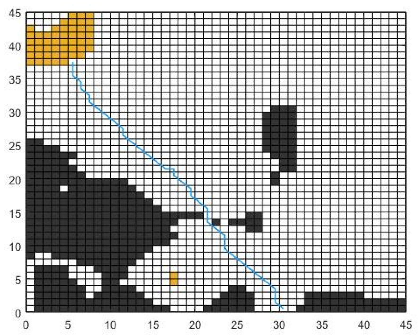
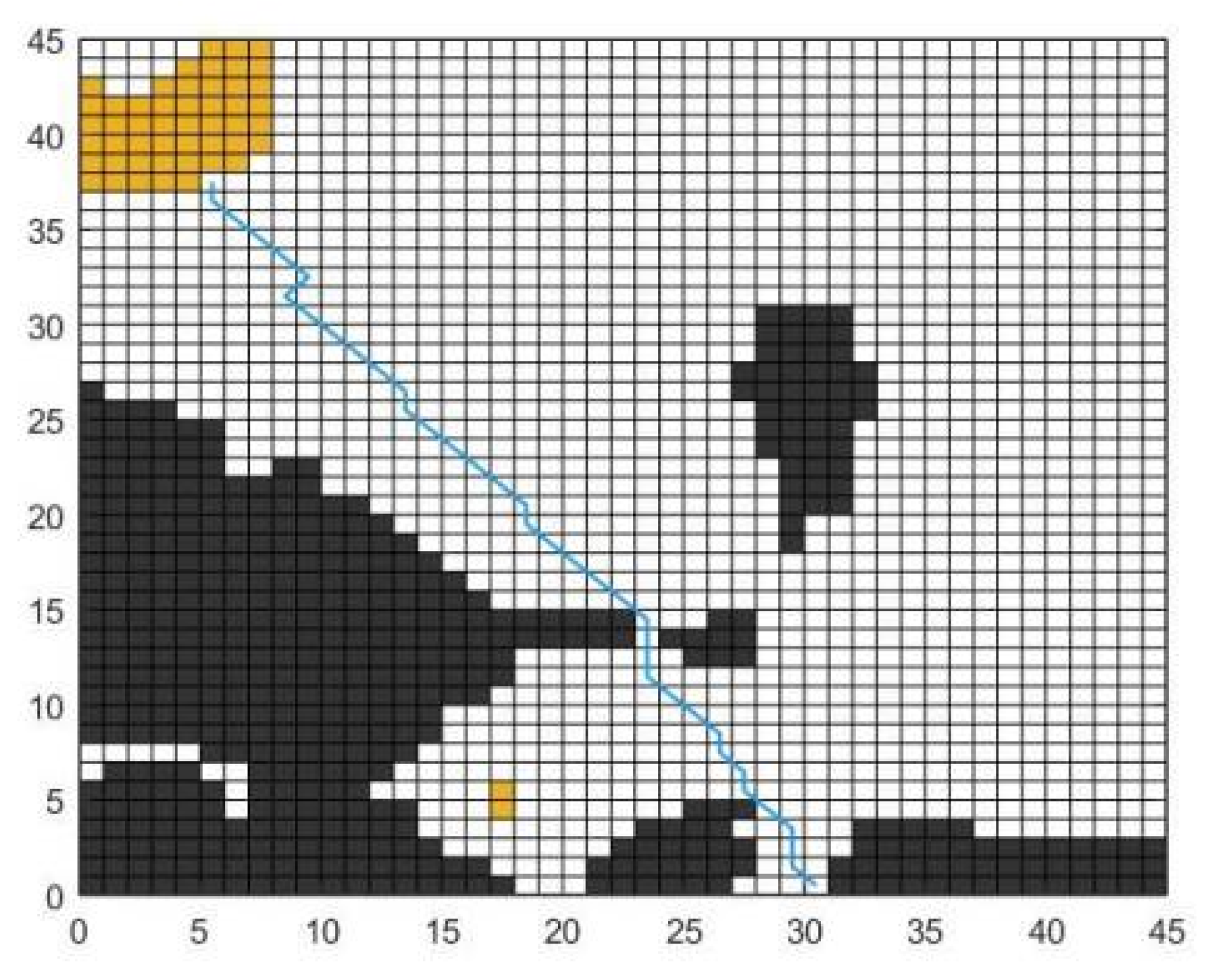
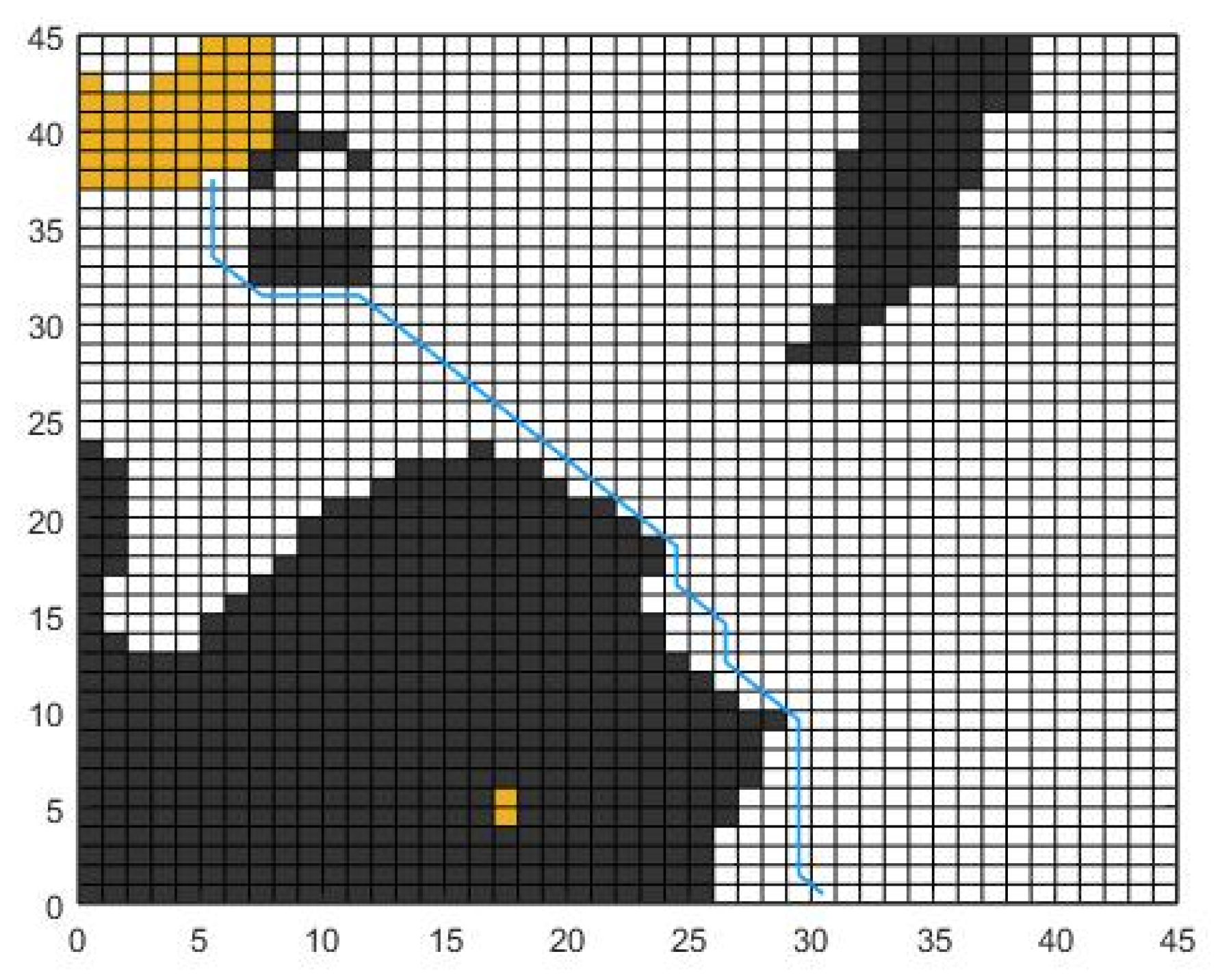
3.1. Experimental Design

In this study, we obtained the meteorological weather data from the European Centre for Medium-Range Weather Forecasts. The meteorological data used in this article include the global wind direction, wind speed, wave direction, and wave height. The resolution of the selected meteorological data is $0.5°\times 0.5°$. We intercepted part of the North Pacific Ocean with sea areas of $137° \mathrm{E}\sim 159° \mathrm{E},15° \mathrm{N}\sim 37° \mathrm{N}$, constructing a grid environment consisting of $45\times 45$ grids. Set the starting point is $139.5° \mathrm{E},33.5° \mathrm{N}$, and the final target is $152° \mathrm{E},15° \mathrm{N}$. The cost of fuel is 856.5 USD per ton. The experimental ship in this study is a bulker called Yu Long Ling. The ship parameters are given in

Table 1. Detailed parameters of the experimental ship.

Dead Weight Ton (t)	The Speed of the Ship (kts)	The Power of the Main Engine (kW)	The Fuel Consumption Rate of the Ship (g/kWh)
32,005	15	6480	159.4

. The initial values of the IMACO algorithm are given in

Table 2. IMACO algorithm parameters.

Parameter	Value
Number of iterations	500
Number of ants	20
The importance of pheromone ($\alpha$)	1
The importance of heuristic factor ($\beta$)	7
Pheromone evaporation coefficient ($\rho$)	0.3
Pheromone increase intensity coefficient ($Q$)	1

.

This study set up two experiments:

• To verify the effectiveness of this algorithm, we designed three shipping companies with different navigation strategies. The IMACO algorithm was used to simulate the optimal routes of different shipping companies. In addition, the voyage distance, total time and fuel consumption cost of the three shipping companies were calculated respectively.
• To verify the advancement of this algorithm, we compared the result of the SACO algorithm with the result of Company A (under the IMACO algorithm). Two indicators of wind speed and wave height in the SACO algorithm were selected to construct the marine risk environment of ships, the wind speed is limited to 12 m/s, and the wave height is limited to 2 m.

3.2. Experimental Results and Analysis

Since there are deviations in the routes of different shipping companies on the same route, we used the TOPSIS method to comprehensively consider the navigation strategies of different companies. First, the two indicators of fuel consumption cost and ship navigation risk of each grid were comprehensively evaluated according to the weight of 1:1, and then the grid map was converted into a score grid map, as shown in Figure 4. Figure 4 shows part of scores in each grid of the map. The higher the value, the more favorable the area is to sail. Second, the navigation strategies of different shipping companies were distinguished with different score boundaries: above the boundary represents the navigable area (white grid area), otherwise, it was the non-navigable area (brown and black grid areas, the brown part is the eastern region of Japan, the black part is the operational obstacle). The values of the score boundaries ($f$) are shown in Equation (13). It can effectively distinguish the operation philosophy of different shipping companies.

$$f=\{\begin{array}{l}4.4,\mathrm{low}-\mathrm{demand}\mathrm{navigation}\mathrm{strategy}\\ 4.7,\mathrm{medium}-\mathrm{demand}\mathrm{navigation}\mathrm{strategy}\\ 4.9,\mathrm{high}-\mathrm{demand}\mathrm{navigation}\mathrm{strategy}\end{array}$$

(13)

According to the IMACO algorithm proposed above, we used MATLAB software to simulate ship route planning for three companies with different navigation strategies. The results are shown in Figure 5, Figure 6 and Figure 7. These results correspond to different shipping companies whose navigation management demands are from low to high, and are represented by A, B, and C. The blue lines are the optimal routes obtained by simulation.

From the results, it is clear that from Figure 5, Figure 6 and Figure 7, the corresponding operational obstacles gradually increase, and the navigation scopes of the corresponding companies gradually narrow. The operational obstacles are characterized by continuous distribution. In addition, it can be seen from Equations (3) and (5) that fuel consumption cost is related to speed, speed is directly related to wind speed and wave height. The distribution of the wind speed and wave height is relatively continuous, so the operational obstacles also have the characteristics of continuous distribution.

Figure 8 shows the route length, voyage time, and fuel consumption cost of three companies. On the whole, there is little difference in the voyage time of the three companies, while there are significant differences in the route length and fuel consumption cost. The route length of the great circle route of company A is 1376.45 nm, the voyage time is 102.16 h, and the fuel consumption cost is 114,525.24 USD. The operational obstacles of Company A hardly hinder the route selection, so the optimal route is obtained with few detours. This is because the navigation management objectives of company A are relatively loose, which is a low-demand navigation strategy. In this strategy, the navigable area is usually the widest and the distance is the shortest, but it will be sailed at higher ship navigation risk and in higher fuel consumption areas. The route length of the great circle route of Company B is 1393.05 nm, the voyage time is 103.37 h, and the fuel consumption cost is 115,868.23 USD. Compared with company A, the operational obstacles of company B have increased significantly. It can be seen that the optimal route shows a certain degree of detour in the middle of the map due to avoiding obstacles. This reflects the fact that the navigation management objectives of company B are relatively strict, which is a medium-demand navigation strategy. This strategy is intermediate between A and C, and has disadvantages: the navigable area is narrow, which creates the possibility of detours, and there is the possibility of sailing at higher ship navigation risk and in higher fuel consumption areas. The route length of the great circle route of company C is 1399.01 nm, the voyage time is 104.23 h, and the fuel consumption cost is 116,781.91 USD. Company C has the most operational obstacles, which will greatly restrict its route selection. In this environment, ships will navigate around obstacles in the middle and near the end of the map. This indicates that company C has the strictest navigation management objectives, which is a high-demand navigation strategy. In this strategy, the navigable area is usually the narrowest, and the route is relatively safe but detours exist.

Traditionally, all shipping companies in the SACO algorithm carry out route planning based on the exact same chart, which will reduce the independence of their route selection and make it difficult for shipping companies to exert their operational advantages. According to the characteristics of different shipping companies, the IMACO algorithm obtains charts with the company’s operating characteristics, which can intuitively reflect the shipping company’s preferences and operating advantages on the charts.

To verify the advancement of the IMACO algorithm, we compare it with the SACO algorithm. Figure 9 shows the route planning result of the SACO algorithm. In addition, we calculate its route length, voyage time, and fuel consumption cost.

Table 3. Comparison of the IMACO algorithm with the SACO algorithm for 4 examples.

Example	Route Length (nm)	Voyage Time (h)	Fuel Consumption Cost (Hundred Dollars)
Company A	1376.45	102.16	1145.25
Company B	1393.05	103.37	1158.68
Company C	1399.01	104.23	1167.82
Contrast experiment	1440.13	106.87	1196.40

shows the difference between the result of the contrast experiment and the results in Figure 8.

From Table 3, we find that the IMACO algorithm is better than the latter in different aspects. Compared with the route planned by Company A, we observed a saving of 63.68 nm in the route length, which is equivalent to saving 4.63% of the total route length; In terms of voyage time, it saves approximately 4.71 h, which is equivalent to 4.61% of the time being saved; in terms of fuel consumption cost, it saves about 5115 USD, which is equivalent to 4.47% of the cost being saved.

This matches the expected results. It can be seen that the IMACO algorithm has great advantages over the SACO algorithm. Therefore, the algorithm has practical significance for shipping companies for saving voyage time and fuel consumption cost.

4. Conclusions

This paper proposed an improved multi-objective ant colony (IMACO) algorithm that comprehensively considers ship navigation risk and fuel consumption cost under complex sea conditions. The main contribution of this algorithm is that different route planning grid maps can be obtained according to the differences in navigation strategies of different shipping companies. In the grid environment, shipping companies can more easily choose routes that meet their own navigation strategies. We calculated the fuel consumption cost and ship navigation risk of each grid, and further used the TOPSIS method to evaluate these two indicators for each grid. Moreover, by both using the algorithm for simulation experiments and comparing it with the traditional single-objective ant colony (SACO) algorithm, we verified the effectiveness and practical significance of the application of the IMACO algorithm. The results show that due to the different strictness of navigation management requirements of different companies, different routes are selected in the same sea area at the same time.

References

1. United Nations Conference on Trade and Development. Review of Maritime Transport 2021; United Nations: New York, NY, USA, 2021. [Google Scholar] [CrossRef]
2. Zhao, W.; Wang, H.; Geng, J.; Hu, W.; Zhang, Z.; Zhang, G. Multi-Objective Weather Routing Algorithm for Ships Based on Hybrid Particle Swarm Optimization. J. Ocean. Univ. China 2022, 21, 28–38. [Google Scholar] [CrossRef]
3. Lindstad, H.; Asbjørnslett, B.E.; Jullumstrø, E. Assessment of profit, cost and emissions by varying speed as a function of sea conditions and freight market. Transp. Res. Part D Transp. Environ. 2013, 19, 5–12. [Google Scholar] [CrossRef]
4. Liu, X.; Li, Y.; Zhang, J.; Zheng, J.; Yang, C. Self-adaptive dynamic obstacle avoidance and path planning for USV under complex maritime environment. IEEE Access 2019, 7, 114945–114954. [Google Scholar] [CrossRef]
5. Park, J.; Kim, N. Two-phase approach to optimal weather routing using geometric programming. J. Mar. Sci. Technol. 2015, 20, 679–688. [Google Scholar] [CrossRef]
6. Mannarini, G.; Coppini, G.; Oddo, P.; Pinardi, N. A prototype of ship routing decision support system for an operational oceanographic service. TransNav Int. J. Mar. Navig. Saf. Sea Transp. 2013, 7, 53–59. [Google Scholar] [CrossRef]
7. Zhou, P.; Wang, H.; Guan, Z. Ship weather routing based on grid system and modified genetic algorithm. In Proceedings of the 2019 IEEE 28th International Symposium on Industrial Electronics (ISIE), Vancouver, BC, Canada, 12–14 June 2019; pp. 647–652. [Google Scholar] [CrossRef]
8. Hanssen, G.L.; James, R.W. Optimum ship routing. J. Navig. 1960, 13, 253–272. [Google Scholar] [CrossRef]
9. Hagiwara, H. Weather Routing of (Sail-Assisted) Motor Vessels. Ph.D. Thesis, Technical University of Delft, Delft, The Netherlands, 1989. [Google Scholar]
10. Szlapczynska, J.; Smierzchalski, R. Adopted isochrone method improving ship safety in weather routing with evolutionary approach. Int. J. Reliab. Qual. Saf. Eng. 2007, 14, 635–645. [Google Scholar] [CrossRef]
11. Roh, M.-I. Determination of an economical shipping route considering the effects of sea state for lower fuel consumption. Int. J. Nav. Archit. Ocean. Eng. 2013, 5, 246–262. [Google Scholar] [CrossRef] [Green Version]
12. Bellman, R. On the theory of dynamic programming. Proc. Natl. Acad. Sci. USA 1952, 38, 716–719. [Google Scholar] [CrossRef]
13. Zoppoli, R. Minimum-time routing as an N-stage decision process. J. Appl. Meteorol. 1972, 11, 429–435. [Google Scholar] [CrossRef]
14. Barber, C.; Sen, P.; Downie, M. Parallel dynamic programming and ship voyage management. Concurr. Pract. Exp. 1994, 6, 673–696. [Google Scholar] [CrossRef]
15. Shao, W.; Zhou, P.; Thong, S.K. Development of a novel forward dynamic programming method for weather routing. J. Mar. Sci. Technol. 2012, 17, 239–251. [Google Scholar] [CrossRef]
16. Skoglund, L.; Kuttenkeuler, J.; Rosén, A.; Ovegård, E. A comparative study of deterministic and ensemble weather forecasts for weather routing. J. Mar. Sci. Technol. 2015, 20, 429–441. [Google Scholar] [CrossRef]
17. Prpić-Oršić, J.; Vettor, R.; Faltinsen, O.M.; Guedes Soares, C. The influence of route choice and operating conditions on fuel consumption and CO2 emission of ships. J. Mar. Sci. Technol. 2016, 21, 434–457. [Google Scholar] [CrossRef]
18. Kuhlemann, S.; Tierney, K. A genetic algorithm for finding realistic sea routes considering the weather. J. Heuristics 2020, 26, 801–825. [Google Scholar] [CrossRef]
19. Du, W.; Li, Y.; Zhang, G.; Wang, C.; Chen, P.; Qiao, J. Estimation of ship routes considering weather and constraints. Ocean. Eng. 2021, 228, 108695. [Google Scholar] [CrossRef]
20. Borén, C.; Castells-Sanabra, M.; Grifoll, M. Ship emissions reduction using weather ship routing optimisation. Proc. Inst. Mech. Eng. 2022. [Google Scholar] [CrossRef]
21. Pan, C.; Zhang, Z.; Sun, W.; Shi, J.; Wang, H. Development of ship weather routing system with higher accuracy using SPSS and an improved genetic algorithm. J. Mar. Sci. Technol. 2021, 26, 1324–1339. [Google Scholar] [CrossRef]
22. Shin, Y.W.; Abebe, M.; Noh, Y.; Lee, S.; Lee, I.; Kim, D.; Bae, J.; Kim, K.C. Near-optimal weather routing by using improved A* algorithm. Appl. Sci. 2020, 10, 6010. [Google Scholar] [CrossRef]
23. Howden, W.E. The sofa problem. Comput. J. 1968, 11, 299–301. [Google Scholar] [CrossRef]
24. Liu, F. Study on the Ship’s Loss-Speed in Wind and Waves. J. Dalian Marit. Univ. 1992, 4, 347–351. (In Chinese) [Google Scholar]
25. Zhang, G.; Wang, H.; Zhao, W.; Guan, Z.; Li, P. Application of improved multi-objective ant colony optimization algorithm in ship weather routing. J. Ocean. Univ. China 2021, 20, 45–55. [Google Scholar] [CrossRef]
26. Colorni, A.; Dorigo, M.; Maniezzo, V. Distributed optimization by ant colonies. In Proceedings of the first European Conference on Artificial Life, Paris, France, 11–13 December 1991; pp. 134–142. [Google Scholar]
Figure 1. Ship route decomposition diagram.
Jmse 10 01212 g001
Figure 2. Ship navigation risk diagram.
Jmse 10 01212 g002
Figure 3. TOPSIS score for part of the grid.
Jmse 10 01212 g003
Figure 4. Part of scores in each grid of the map.
Jmse 10 01212 g004
Figure 5. The result of company A.
Jmse 10 01212 g005
Figure 6. The result of company B.
Jmse 10 01212 g006
Figure 7. The result of company C.
Jmse 10 01212 g007
Figure 8. Comparison of three companies in route length, voyage time, and fuel consumption cost.
Jmse 10 01212 g008
Figure 9. The result of the contrast experiment.
Jmse 10 01212 g009