
Discerning Discretization for Unmanned Underwater Vehicles DC Motor Control


Abstract
:1. Introduction
1.1. Research Lineage from the M.I.T. Rule to Regression
1.2. Least Squares Variations
1.3. Physics-Based Utilization of Governing Differential Equations
1.4. Discretization
2. Materials and Methods
2.1. Modeling DC Motor Dynamics and Designing Control Strategies
2.2. Discretization Methods
3. Results
4. Discussion
Author Contributions
Funding
Institutional Review Board Statement
Informed Consent Statement
Data Availability Statement
Conflicts of Interest
Appendix A
| %% Investigating the effects of discretization for control of DC motors using deterministic artificial intelligence clear; close all; clc; rng(100); %% Setting up the problem: % Generate reference input as a square wave maxtime = 200; U_ctrl = zeros(1,201); for i = 1:length(U_ctrl) if (mod(floor(i/20),2) == 0) U_ctrl(i) = 1; else U_ctrl(i) = 0; end end U_ctrl_traj = zeros(1,length(U_ctrl)); check = 1; next_run = 0; for i = 1:length(U_ctrl)-1 if (check) U_ctrl_traj(i) = U_ctrl(i); delta = U_ctrl(i + 1)-U_ctrl(i); i_last = i; val_last = U_ctrl(i); end if (delta ~= 0) check = 0; if (next_run) U_ctrl_traj(i) = val_last + delta/2*(1 + (sin(0.2*pi*(i-i_last)-pi/2))); end next_run = 1; if (U_ctrl_traj(i) == U_ctrl(i) && (i ~= i_last)) check = 1; next_run = 0; end end end U_ctrl = U_ctrl(1:200); % System modeling Ts = 0.7; TF_c = tf(1,[1 1 0]); % continuous transfer function TF_d = c2d(TF_c,Ts,‘foh’); % discrete transfer function % Hd = tf([0 0.1065 0.0902],poly([1.1 0.8]),0.5); % analytic discrete transfer function % Hd = tf([0 0.0902 0.06461],[1 -1.213 0.3679],0.5); % offline discrete transfer function Num_coef = [TF_d.Numerator{1,1}(1,1),TF_d.Numerator{1,1}(1,2),TF_d.Numerator{1,1}(1,3)]; Denom_coef = [TF_d.Denominator{1,1}(1,1),TF_d.Denominator{1,1}(1,2),TF_d.Denominator{1,1}(1,3)]; nzeros = 5; noise_std = 25; Noise_distr = 1/noise_std*randn(1,maxtime + nzeros); %% Algorithm for Recursive Least Squares (RLS): % Setup system parameters b_1 = 0.2; b_0 = 0.1; a_2 = 0; a_1 = 0; B_m = [0 0.1065 0.0902]; A_m = poly([0.2 + 0.2j 0.2-0.2j]); a_0 = 0; a_m2 = A_m(3); a_m1 = A_m(2); time = zeros(1, nzeros); Y_RLS = zeros(1, nzeros); Ym_RLS = zeros(1, nzeros); U_RLS = ones(1, nzeros); Uc_RLS = [ones(1, nzeros), U_ctrl]; Pmatrix = [100 0 0 0;0 100 0 0;0 0 1 0;0 0 0 1]; THETA_hat_RLS(:,1) = [-a_1 -a_2 b_0 b_1]’; alpha = 0.5; beta = []; gamma = 1.2; lambda = 1.0; Rmatrix = []; %%%%%%%%%%%%%%%%%%%%%%%RECURSIVE LEAST SQUARES%%%%%%%%%%%%%%%%%%%%%%%%%%%%% for i = 1:1:maxtime t = i + nzeros; phi_vec = []; time(t) = i; Y_RLS(t) = [-Denom_coef(2) -Denom_coef(3) Num_coef(2) Num_coef(3)]*[Y_RLS(t-1) Y_RLS(t-2) U_RLS(t-1) U_RLS(t-2)]’+... Noise_distr(t-1) + Noise_distr(t-2); Ym_RLS(t) = [-A_m(2) -A_m(3) B_m(2) B_m(3)]*[Ym_RLS(t-1) Ym_RLS(t-2) Uc_RLS(t-1) Uc_RLS(t-2)]’; BETA = (A_m(1) + A_m(2) + A_m(3))/(b_0 + b_1); beta = [beta BETA]; % Implementation of the RLS method phi_vec = [Y_RLS(t-1) Y_RLS(t-2) U_RLS(t-1) U_RLS(t-2)]’; Kmatrix = Pmatrix*phi_vec*1/(lambda + phi_vec’*Pmatrix*phi_vec); Pmatrix = Pmatrix - Pmatrix*phi_vec*inv(1+phi_vec’*Pmatrix*phi_vec)*phi_vec’*Pmatrix/lambda; % RLS-EF error(i) = Y_RLS(t) - phi_vec’*THETA_hat_RLS(:,i); THETA_hat_RLS(:,i + 1) = THETA_hat_RLS(:,i) + Kmatrix*error(i); a_2 = -THETA_hat_RLS(2,i + 1); a_1 = -THETA_hat_RLS(1,i + 1); b_1 = THETA_hat_RLS(4,i + 1); b_0 = THETA_hat_RLS(3,i + 1); Bf(:,i) = [b_0 b_1]’; Af(:,i) = [1 a_1 a_2]’; % Determine R,S, & T for CONTROLLER r_1 = (b_1/b_0) + (b_1^2-a_m1*b_0*b_1 + a_m2*b_0^2)*(-b_1 + a_0*b_0)/(b_0*(b_1^2-a_1*b_0*b_1 + a_2*b_0^2)); s_0 = b_1*(a_0*a_m1-a_2-a_m1*a_1 + a_1^2 + a_m2-a_1*a_0)/(b_1^2-a_1*b_0*b_1 + a_2*b_0^2)... +b_0*(a_m1*a_2-a_1*a_2-a_0*a_m2 + a_0*a_2)/(b_1^2-a_1*b_0*b_1 + a_2*b_0^2); s_1 = b_1*(a_1*a_2-a_m1*a_2 + a_0*a_m2-a_0*a_2)/(b_1^2-a_1*b_0*b_1 + a_2*b_0^2) + ... b_0*(a_2*a_m2-a_2^2-a_0*a_m2*a_1 + a_0*a_2*a_m1)/(b_1^2-a_1*b_0*b_1 + a_2*b_0^2); S = [s_0 s_1]; R = [1 r_1]; Rmatrix = [Rmatrix r_1]; T = BETA*[1 a_0]; % Calculate control signal U_RLS(t) = [T(1) T(2) -R(2) -S(1) -S(2)]*[Uc_RLS(t) Uc_RLS(t-1) U_RLS(t-1) Y_RLS(t) Y_RLS(t-1)]’; U_RLS(t) = 1.3*[T(1) T(2) -R(2) -S(1) -S(2)]*[Uc_RLS(t) Uc_RLS(t-1) U_RLS(t-1) Y_RLS(t) Y_RLS(t-1)]’; end %%%%%%%%%%%%%%%%%%%%%%%%END OF RECURSIVE LEAST SQUARES%%%%%%%%%%%%%%%%%%%%% %% Algorithm for Autoregressive moving average (ARMA): % Setup system parameters b_1 = 0.2; b_0 = 0.01; a_2 = 0; a_1 = 0; B_m = [0 0.1065 0.0902]; A_m = poly([0.2 + 0.2j 0.2-0.2j]); a_m2 = A_m(3); a_m1 = A_m(2); a_0 = 0; n = 8; time = zeros(1, nzeros); Y_ARMA = zeros(1, nzeros); U_ARMA = ones(1, nzeros); Uc_ARMA = [ones(1, nzeros), U_ctrl]; THETA_hat_ARMA = zeros(4, maxtime); beta = []; THETA_hat_ARMA(:,1) = [-a_1 -a_2 b_0 b_1]’; Pmatrix = 10000*eye(n); Pmatrix(1,1) = 1000; Pmatrix(2,2) = 100; Pmatrix(3,3) = 100; Pmatrix(4,4) = 10000; Pmatrix(5,5) = 1000; Pmatrix(6,6) = 100; phi_vec = []; Rmatrix = []; lambda = 1; %%%%%%%%%%%%%%%%%%%%%%AUTOREGRESSIVE MOVING AVERAGE%%%%%%%%%%%%%%%%%%%%%%%% for i = 1:1:maxtime t = i + nzeros; time(t) = i; Y_ARMA(t) = [-Denom_coef(2) -Denom_coef(3) Num_coef(2) Num_coef(3)]*... [Y_ARMA(t-1) Y_ARMA(t-2) U_ARMA(t-1) U_ARMA(t-2)]’ + ... Noise_distr(t-1) + Noise_distr(t-2); % Generate truth output BETA = (A_m(1) + A_m(2) + A_m(3))/(b_0 + b_1); beta = [beta BETA]; phi_vec = [phi_vec; Y_ARMA(t-1) Y_ARMA(t-2) U_ARMA(t-1) U_ARMA(t-2)]; if (i > 3) THETA_hat_ARMA(:,i + 1) = inv(phi_vec’*phi_vec)*phi_vec’*Y_ARMA(1 + nzeros:t)’; else THETA_hat_ARMA(:,i + 1) = THETA_hat_ARMA(:, i); end a_2 = -THETA_hat_ARMA(2,i + 1); a_1 = -THETA_hat_ARMA(1,i + 1); b_1 = THETA_hat_ARMA(4,i + 1); b_0 = THETA_hat_ARMA(3,i + 1); % Update A & B coefficients % Save final coefficient values for comparison with real values to obtain epsilon errors B_f(:,i) = [b_0 b_1]’; A_f(:,i) = [1 a_1 a_2]’; % Determine R, S, & T for CONTROLLER r_1 = (b_1/b_0) + (b_1^2-a_m1*b_0*b_1 + a_m2*b_0^2)*(-b_1 + a_0*b_0)/(b_0*(b_1^2-a_1*b_0*b_1 + a_2*b_0^2)); s_0 = b_1*(a_0*a_m1-a_2-a_m1*a_1 + a_1^2 + a_m2-a_1*a_0)/(b_1^2-a_1*b_0*b_1 + a_2*b_0^2) + ... b_0*(a_m1*a_2-a_1*a_2-a_0*a_m2 + a_0*a_2)/(b_1^2-a_1*b_0*b_1 + a_2*b_0^2); s_1 = b_1*(a_1*a_2-a_m1*a_2 + a_0*a_m2-a_0*a_2)/(b_1^2-a_1*b_0*b_1 + a_2*b_0^2) + ... b_0*(a_2*a_m2-a_2^2-a_0*a_m2*a_1 + a_0*a_2*a_m1)/(b_1^2-a_1*b_0*b_1 + a_2*b_0^2); S = [s_0 s_1]; R = [1 r_1]; Rmatrix = [Rmatrix r_1]; T = BETA*[1 a_0]; % Calculate control signal U_ARMA(t) = [T(1) T(2) -R(2) -S(1) -S(2)]*[Uc_ARMA(t) Uc_ARMA(t-1) U_ARMA(t-1) Y_ARMA(t) Y_ARMA(t-1)]’; % Arbitrarily increased to duplicate text U_ARMA(t) = 1.3*[T(1) T(2) -R(2) -S(1) -S(2)]*[Uc_ARMA(t) Uc_ARMA(t-1) U_ARMA(t-1) Y_ARMA(t) Y_ARMA(t-1)]’; end %%%%%%%%%%%%%%%%%%%END OF AUTOREGRESSIVE MOVING AVERAGE%%%%%%%%%%%%%%%%%%%% %% Algorithm for Extended Least Squares (ELS): % Setup system parameters b_1 = 0.2; b_0 = 0.01; a_2 = 0; a_1 = 0; B_m = [0 0.1065 0.0902]; A_m = poly([0.2 + 0.2j 0.2-0.2j]); a_m2 = A_m(3); a_m1 = A_m(2); a_0 = 0; n = 8; time = zeros(1, nzeros); Y_ELS = zeros(1, nzeros); Ym_ELS = zeros(1, nzeros); U_ELS = ones(1, nzeros); Uc_ELS= [ones(1, nzeros), U_ctrl]; THETA_hat_ELS(:,1) = [-a_1 -a_2 b_0 b_1]’; beta = []; % initialize P(t), THETA_hat(t) & Beta epsln = [zeros(1, nzeros + maxtime)]; Pmatrix = 10000*eye(n); Pmatrix(1,1) = 1000; Pmatrix(2,2) = 100; Pmatrix(3,3) = 100; Pmatrix(4,4) = 10000; Pmatrix(5,5) = 1000; Pmatrix(6,6) = 100; Rmatrix = []; lambda = 1; theta_hat_els = zeros(n, 1); %%%%%%%%%%%%%%%%%%%%EXTENDED LEAST SQUARES%%%%%%%%%%%%%%%%%%%%%%%%%%%%%%%% for i = 1:1:maxtime t = i + nzeros; time(t) = i; phi_vec = []; k = i + nzeros; Y_ELS(t) = [-Denom_coef(2) -Denom_coef(3) Num_coef(2) Num_coef(3)]*... [Y_ELS(t-1) Y_ELS(t-2) U_ELS(t-1) U_ELS(t-2)]’ + ... Noise_distr(t-1) + Noise_distr(t-2); % generate truth output Ym_ELS(t) = [-A_m(2) -A_m(3) B_m(2) B_m(3)]*... [Ym_ELS(t-1) Ym_ELS(t-2) Uc_ELS(t-1) Uc_ELS(t-2)]’; BETA = (A_m(1) + A_m(2) + A_m(3))/(b_0 + b_1); beta = [beta BETA]; phi_vec = [Y_ELS(t-1) Y_ELS(t-2) U_ELS(t-1) U_ELS(t-2) epsln(t) epsln(t-1) epsln(t-2) epsln(k-3)]’; Kmatrix = Pmatrix*phi_vec*1/(1 + phi_vec’*Pmatrix*phi_vec); Pmatrix = Pmatrix-Pmatrix*phi_vec*pinv(1 + phi_vec’*Pmatrix*phi_vec)*phi_vec’*Pmatrix; error(i) = Y_ELS(k)-phi_vec’*theta_hat_els(:, i); theta_hat_els(:, i + 1) = theta_hat_els(:, i) + Kmatrix*error(i); epsln(k) = Y_ELS(k) - phi_vec’*theta_hat_els(:, i + 1); % Posterior Residual formulation THETA_hat_ELS(:, i + 1) = theta_hat_els(1:4, i + 1); % Update A & B coefficients a_1 = -THETA_hat_ELS(1,i + 1); a_2 = -THETA_hat_ELS(2,i + 1); b_0 = THETA_hat_ELS(3,i + 1); b_1 = THETA_hat_ELS(4,i + 1); % Store final A and B for comparison with real A&B to generate epsilon errors A_f(:,i) = [1 a_1 a_2]’; B_f(:,i) = [b_0 b_1]’; r_1 = (b_1/b_0) + (b_1^2-a_m1*b_0*b_1 + a_m2*b_0^2)*(-b_1 + a_0*b_0)/(b_0*(b_1^2-a_1*b_0*b_1 + a_2*b_0^2)); s_0 = b_1*(a_0*a_m1-a_2-a_m1*a_1 + a_1^2 + a_m2-a_1*a_0)/(b_1^2-a_1*b_0*b_1 + a_2*b_0^2) + ... b_0*(a_m1*a_2-a_1*a_2-a_0*a_m2 + a_0*a_2)/(b_1^2-a_1*b_0*b_1 + a_2*b_0^2); s_1 = b_1*(a_1*a_2-a_m1*a_2 + a_0*a_m2-a_0*a_2)/(b_1^2-a_1*b_0*b_1 + a_2*b_0^2) + ... b_0*(a_2*a_m2-a_2^2-a_0*a_m2*a_1 + a_0*a_2*a_m1)/(b_1^2-a_1*b_0*b_1 + a_2*b_0^2); S = [s_0 s_1]; R = [1 r_1]; Rmatrix = [Rmatrix r_1]; T = BETA*[1 a_0]; % Calculate control signal U_ELS(t) = [T(1) T(2) -R(2) -S(1) -S(2)]*[Uc_ELS(t) Uc_ELS(t-1) U_ELS(t-1) Y_ELS(t) Y_ELS(t-1)]’; U_ELS(t) = 1.3*[T(1) T(2) -R(2) -S(1) -S(2)]*[Uc_ELS(t) Uc_ELS(t-1) U_ELS(t-1) Y_ELS(t) Y_ELS(t-1)]’; end %%%%%%%%%%%%%%%%%%%%%%%%%%END OF EXTENDED LEAST SQUARES%%%%%%%%%%%%%%%%%%%% %% Algorithm for Deterministic Artificial Intelligence (DAI): % Create command signal nzeros = 5; time = zeros(1, nzeros); U_DAI = ones(1,nzeros); Y_DAI = zeros(1, nzeros); % initialize ouput vectors t = 0:200; hvy_m = [zeros(1, nzeros) U_ctrl_traj]; eb = Y_DAI(1) - hvy_m(1); kd = 6.0; kp = 2.0; err = 0; phid = []; hatvec = zeros(4,1); Rmatrix = []; ustar = []; %%%%%%%%%%%%%%%%%%%%%DETERMINISTIC AI%%%%%%%%%%%%%%%%%%%%%%%%%%%%%%%%%%%%% % Loop through the output data Y(t) for i = 1:1:maxtime + 1 t = i + nzeros; time(t) = i; d_e = err - eb; u = kp*err + kd*d_e; U_DAI(t-1) = u; Y_DAI(t) = [-Denom_coef(2) -Denom_coef(3) Num_coef(2) Num_coef(3)]*... [Y_DAI(t-1) Y_DAI(t-2) U_DAI(t-1) U_DAI(t-2)]’ + ... Noise_distr(t-1) + Noise_distr(t-2); phid = [phid; Y_DAI(t) -Y_DAI(t-1) Y_DAI(t-2) -U_DAI(t-2)]; ustar = [ustar; u]; newest = phid\ustar; hatvec(:,i) = newest; eb = err; err = hvy_m(t)-Y_DAI(t); end %%%%%%%%%%%%%%%%%%%%%%%%%END OF DETERMINISTIC AI%%%%%%%%%%%%%%%%%%%%%%%%%%% THETA_hat_DAI = [hatvec(2,:)./hatvec(1,:); hatvec(3,:)./hatvec(1,:);... ones(1,201)./hatvec(1,:); hatvec(4,:)./hatvec(1,:)]; mean_abs_error_DAI = mean(abs(traj_Uc - Y_DAI(1,6:end))) mean_abs_error_ELS = mean(abs(Uc - Y_ELS(1,6:end))) mean_abs_error_ARMA = mean(abs(Uc - Y_ARMA(1,6:end))) mean_abs_error_RLS = mean(abs(Uc - Y_RLS(1,6:end))) std_error_DAI = std(traj_Uc - Y_DAI(1,6:end)) std_error_ELS = std(Uc - Y_ELS(1,6:end)) std_error_ARMA = std(Uc - Y_ARMA(1,6:end)) std_error_RLS = std(Uc - Y_RLS(1,6:end)) %% Plotting results: figure(); hold on; grid on; plot(time(1,1:205), Y_RLS,‘g--*’); plot(time(1,1:205), Y_ARMA,‘b--o’); plot(time(1,1:205), Y_ELS,‘r-.’); plot(time, Y_DAI,‘m:’); xlabel(‘Time step (in sec)’); ylabel(‘Output (Y)’); plot(time(1:200),Uc,‘k-’); axis([0 50,-0.5 2.0]); % legend(‘RLS’,‘ARMA’,‘ELS’,‘DAI’,‘Reference Input’); title("Discretization using First Order Hold and Sample Time "+ ts); PrepFigPresentation(gcf); function PrepFigPresentation(fignum) % Prepares a figure for presentations % Font size: 10 % Font Name: Times % LineWidth: 2 % figure(fignum); fig_children = get(fignum,‘children’); % find all sub-plots for i = 1:length(fig_children) set(fig_children(i),‘FontSize’,10); set(fig_children(i),‘FontName’,‘times’); fig_children_children = get(fig_children(i),‘Children’); set(fig_children_children,‘LineWidth’,2); end end |
Appendix B
| Low Voltage DC Motors | |||||
| Diameter (mm) | Input Voltage (V) | No Load Speed (rpm) | Maximum Efficiency (%) | Stall Torque (mNm) | Max. Output Power (W) |
| 15.5 | 5.0 | 12,623 | 50 | 2.09 | 0.69 |
| 20.4 | 13.0 | 25,000 | 65 | 20.00 | 15.00 |
| 20.4 | 2.4 | 6200 | 65 | 8.00 | 1.30 |
| 24.2 | 2.4 | 7000 | 70 | 26.00 | 5.00 |
| 24.2 | 1.2 | 7800 | 60 | 12.00 | 2.50 |
| 24.2 | 24.0 | 26,000 | 70 | 85.00 | 60.00 |
| 24.0 | 21.0 | 30,000 | 60 | 40.00 | 32.00 |
| 24.4 | 12.0 | 8200 | 62 | 25.50 | 5.50 |
| 27.5 | 24.0 | 7200 | 55 | 20.00 | 4.00 |
| 27.5 | 41.0 | 18,000 | 65 | 38.00 | 18.00 |
| 27.5 | 18.0 | 9987 | 57 | 39.24 | 10.20 |
| 27.5 | 39.0 | 21,000 | 70 | 70.00 | 40.00 |
| 27.5 | 24.0 | 22,000 | 70 | 60.00 | 35.00 |
| 27.5 | 7.2 | 17,230 | 64 | 114.86 | 51.24 |
| 27.5 | 36.0 | 11,000 | 70 | 90.00 | 25.00 |
| 27.5 | 28.0 | 19,000 | 75 | 140.00 | 70.00 |
| 29.0 | 42.0 | 6400 | 64 | 92.00 | 15.50 |
| 42.3 | 18.0 | 20,950 | 78 | 1175.03 | 644.74 |
| 48.0 | 14.4 | 20,120 | 66 | 787.72 | 415.00 |
| 48.0 | 18.0 | 20,281 | 69 | 656.65 | 348.79 |
| 48.0 | 18.0 | 19,600 | 66 | 1055.00 | 542.00 |
| 48.0 | 18.0 | 22,500 | 76 | 1400.00 | 830.00 |
| High Voltage DC Motors | |||||
| Diameter (mm) | Input Voltage (V) | No Load Speed (rpm) | Maximum Efficiency (%) | Torque @ Max. Efficiency (mNm) | Speed @ Maximum Efficiency (rpm) |
| 35.8 | 60.0 | 8600 | 70 | 25.00 | 7400 |
| 45.0 | 230.0 | 15,600 | 65 | 92.00 | 11,500 |
| 52.4 | 120.0 | 11,000 | 64 | 155.00 | 8200 |
References
- Liu, Z.; Zhuang, X.; Wang, S. Speed Control of a DC Motor using BP Neural Networks. In Proceedings of the 2003 IEEE Conference on Control Applications, Istanbul, Turkey, 25–25 June 2003; pp. 832–835. [Google Scholar]
- Mishra, M. Speed Control of DC Motor Using Novel Neural Network Configuration. Bachelor’s Thesis, National Institute of Technology, Rourkela, India, 2009. [Google Scholar]
- Hernández-Alvarado, R.; García-Valdovinos, L.G.; Salgado-Jiménez, T.; Gómez-Espinosa, A.; Fonseca-Navarro, F. Neural Network-Based Self-Tuning PID Control for Underwater Vehicles. Sensors 2016, 16, 1429. [Google Scholar] [CrossRef] [PubMed] [Green Version]
- Rashwan, A. An Indirect Self-Tuning Speed Controller Design for DC Motor Using A RLS Principle. In Proceedings of the 21st International Middle East Power Systems Conference (MEPCON), Cairo, Egypt, 17–19 December 2019; pp. 633–638. [Google Scholar]
- U.S. Naval Forces Southern Command|Navy Deploys Unmanned Submersibles in Argentine Submarine Search. 21 November 2017. Available online: https://www.defense.gov/News/News-Stories/Article/Article/1378119/navy-deploys-unmanned-submersibles-in-argentine-submarine-search/ (accessed on 9 February 2023).
- Rees, C. Maxon Launches High Torque DC Brushless Motors. 5 May 2015. Available online: https://www.unmannedsystemstechnology.com/2015/05/maxon-launches-high-torque-dc-brushless-motors/ (accessed on 19 December 2022).
- Department of Defense Photographs and Imagery, Unless Otherwise Noted, Are in the Public Domain. Available online: https://www.defense.gov/Help-Center/Article/Article/2762906/use-of-department-of-defense-imagery/#:~:text=Department%20of%20Defense%20photographs%20and,use%2C%20subject%20to%20specific%20guidelines (accessed on 9 February 2023).
- Available online: https://www.maxongroup.com/maxon/view/content/underwater-drive-systems (accessed on 10 February 2023).
- Slotine, J.; Benedetto, M. Hamiltonian adaptive control on spacecraft. IEEE Trans. Autom. Control 1990, 35, 848–852. [Google Scholar] [CrossRef]
- Slotine, J.; Weiping, L. Applied Nonlinear Control; Prentice Hall: Englewood Cliffs, NJ, USA, 1991. [Google Scholar]
- Fossen, T. Comments on “Hamiltonian Adaptive Control of Spacecraft”. IEEE Trans. Autom. Control 1993, 38, 671–672. [Google Scholar] [CrossRef]
- Åström, K.; Wittenmark, B. On the Control of Constant but Unknown Systems. In Proceedings of the 5th IFAC World Congress, Paris, France, 12–17 June 1972. [Google Scholar]
- Åström, K.; Wittenmark, B. On self-tuning regulators. Automatica 1973, 9, 185–199. [Google Scholar] [CrossRef]
- Åström, K.; Wittenmark, B. Adaptive Control; Addison-Wesley: Boston, FL, USA, 1995; pp. 90–135. [Google Scholar]
- Sands, T.; Kim, J.; Agrawal, B. Improved Hamiltonian Adaptive Control of spacecraft. In Proceedings of the 2009 IEEE Aerospace conference, Big Sky, MT, USA, 7–14 March 2009. [Google Scholar]
- Sheng, M.; Alvi, M.; Lorenz, R. GMR-based Integrated Current Sensing in SiC Power Modules with Phase Shift Error Reduction. IEEE J. Emerg. Sel. Top. Power Electron. 2022, 10, 3477–3487. [Google Scholar] [CrossRef]
- Sands, T. Development of Deterministic Artificial Intelligence for Unmanned Underwater Vehicles (UUV). J. Mar. Sci. Eng. 2020, 8, 578. [Google Scholar] [CrossRef]
- Sands, T. Control of DC Motors to Guide Unmanned Underwater Vehicles. Appl. Sci. 2021, 11, 2144. [Google Scholar] [CrossRef]
- Shah, R.; Sands, T. Comparing Methods of DC Motor Control for UUVs. Appl. Sci. 2021, 11, 4972. [Google Scholar] [CrossRef]
- Mareels, I.; Anderson, B.; Bitmead, R.; Bodson, M.; Sastry, S. Revisiting the Mit Rule for Adaptive Control. IFAC Proc. Vol. 1987, 20, 161–166. [Google Scholar] [CrossRef]
- Sprott, D. Gauss’s contribution to statistics. Hist. Math. 1978, 5, 183–203. [Google Scholar] [CrossRef] [Green Version]
- Sands, T.; Kim, J.; Agrawal, B. Spacecraft fine tracking pointing using adaptive control. In Proceedings of the 58th International Astronautical Congress, Hyderabad, India, 24–28 September 2007; International Astronautical Federation: Paris, France, 2007. [Google Scholar]
- Smeresky, B.; Rizzo, A.; Sands, T. Optimal Learning and Self-Awareness versus PDI. Algorithms 2020, 13, 23. [Google Scholar] [CrossRef] [Green Version]
- Zhai, H.; Sands, T. Controlling Chaos in Van Der Pol Dynamics Using Signal-Encoded Deep Learning. Mathematics 2022, 10, 453. [Google Scholar] [CrossRef]
- Zhai, H.; Sands, T. Comparison of Deep Learning and Deterministic Algorithms for Control Modeling. Sensors 2022, 22, 6362. [Google Scholar] [CrossRef] [PubMed]
- Åström, K.; Apkarian, J.; Lacheray, H. Quanser Engineering Trainer (QET) Series: USB QICii Laboratory Workbook, DC Motor Control Trainer (DCMCT) Student Workbook. Available online: http://class.ece.iastate.edu/ee476/motion/Main_manual.pdf (accessed on 13 February 2023).


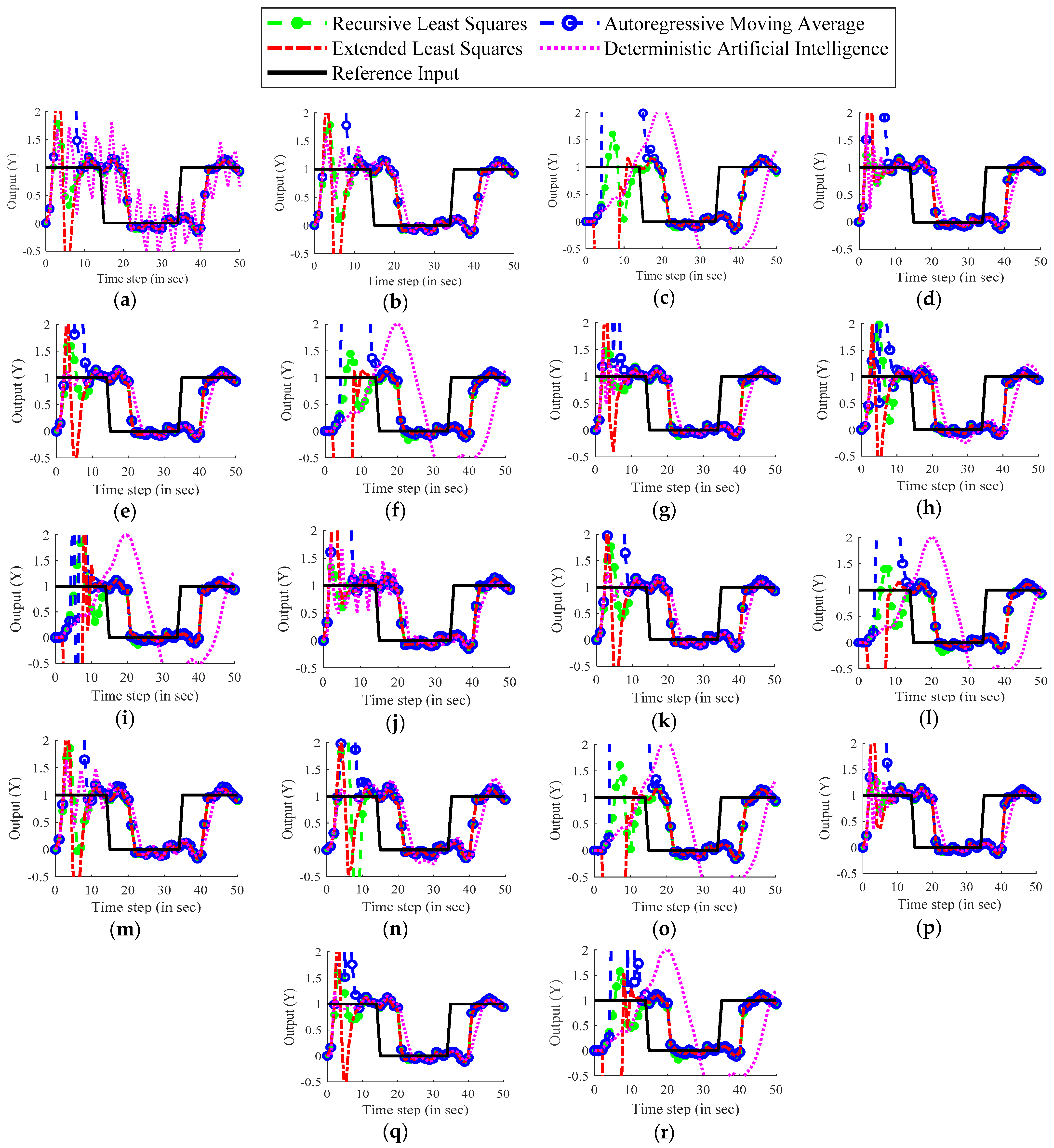
| Plot | Description | Plot | Description | Plot | Description |
|---|---|---|---|---|---|
| (a) | (b) | (c) | |||
| (d) | (e) | (f) | |||
| (g) | (h) | (i) | |||
| (j) | (k) | (l) | |||
| (m) | (n) | (o) | |||
| (p) | (q) | (r) |
| Sample Time (s) | ZOH | FOH | Impulse Invariant Mapping | Tustin Approximation | Zero-Pole Matching Equivalents | Least Squares |
|---|---|---|---|---|---|---|
| 0.8 | -- | -- | -- | 0.1041/0.1646 | -- | -- |
| 0.7 | -- | 0.0840/0.1430 | -- | 0.0894/0.1322 | -- | -- |
| 0.6 | 0.1969/0.2683 | 0.0886/0.1297 | -- | 0.0996/0.1403 | -- | 0.0912/0.1451 |
| 0.5 | 0.1137/0.1612 | 0.1083/0.1513 | 0.0967/0.1437 | 0.1209/0.1658 | 0.1219/0.1722 | 0.0998/0.1416 |
| 0.4 | 0.1408/0.1897 | 0.1453/0.1953 | 0.1179/0.1628 | 0.1604/0.2141 | 0.1434/0.1932 | 0.1329/0.1802 |
| 0.3 | 0.2018/0.2647 | 0.2148/0.2771 | 0.1782/0.2331 | 0.2341/0.3012 | 0.2037/0.2669 | 0.1983/0.2571 |
| 0.2 | 0.3405/0.4225 | 0.3691/0.4512 | 0.3169/0.3903 | 0.3981/0.4849 | 0.3415/0.4238 | 0.3452/0.4232 |
| 0.1 | 0.8467/0.9812 | 0.8708/1.0032 | 0.8045/0.9288 | 0.9040/1.0405 | 0.8474/0.9822 | 0.8413/0.9698 |
Disclaimer/Publisher’s Note: The statements, opinions and data contained in all publications are solely those of the individual author(s) and contributor(s) and not of MDPI and/or the editor(s). MDPI and/or the editor(s) disclaim responsibility for any injury to people or property resulting from any ideas, methods, instructions or products referred to in the content. |
© 2023 by the authors. Licensee MDPI, Basel, Switzerland. This article is an open access article distributed under the terms and conditions of the Creative Commons Attribution (CC BY) license (https://creativecommons.org/licenses/by/4.0/).
Share and Cite
Menezes, J.; Sands, T. Discerning Discretization for Unmanned Underwater Vehicles DC Motor Control. J. Mar. Sci. Eng. 2023, 11, 436. https://doi.org/10.3390/jmse11020436
Menezes J, Sands T. Discerning Discretization for Unmanned Underwater Vehicles DC Motor Control. Journal of Marine Science and Engineering. 2023; 11(2):436. https://doi.org/10.3390/jmse11020436
Chicago/Turabian StyleMenezes, Jovan, and Timothy Sands. 2023. "Discerning Discretization for Unmanned Underwater Vehicles DC Motor Control" Journal of Marine Science and Engineering 11, no. 2: 436. https://doi.org/10.3390/jmse11020436
APA StyleMenezes, J., & Sands, T. (2023). Discerning Discretization for Unmanned Underwater Vehicles DC Motor Control. Journal of Marine Science and Engineering, 11(2), 436. https://doi.org/10.3390/jmse11020436