Trajectory Tracking Nonlinear Controller for Underactuated Underwater Vehicles Based on Velocity Transformation

Abstract

This paper proposes an algorithm that performs the task of tracking the desired trajectory for underactuated marine vehicles (primarily underwater) that move horizontally. The control scheme, which takes into account model inaccuracies and external disturbances, was designed using the quantities obtained after the transformation of the dynamic equations of motion resulting from the decomposition of the inertia matrix. This, in turn, led to the equation of dynamics with a diagonal inertia matrix. A specific feature of the offered controller is its dual role. It not only allows tracking the desired trajectory, but at the same time, makes it possible to estimate the impact of dynamic couplings when the vehicle is in motion. Such an approach to the tracking task is important at the initial design stage when the choice of the control algorithm has not yet been decided and experimental tests have not been performed. This is feasible because the new variables after the velocity transformation include not only vehicle parameters, but also actual velocities and forces. Therefore, it is also possible to track the original variables. The theoretical results were followed up with simulation tests conducted on a model with three degrees of freedom for two underwater vehicles.

1. Introduction

The issues of the control of underactuated marine and especially underwater vehicles have been of interest to researchers for many years. The problems that arise are not only the lack of at least one control signal, but also the limitations of the remaining propulsion, speed, and uncertainty of the parameters and external disturbances. Among the various solutions to the problems of controlling the motion of various marine vehicles, tracking control that allows the system to achieve the desired trajectory with acceptable efficiency seems attractive. The present work was limited only to the implementation of trajectory tracking in planar motion; hence, the literature cited relates to this class of vehicles.

Very often, tracking controllers are designed under the assumption that the model has a diagonal inertia matrix with, therefore, no inertial couplings. Since such a model is very approximate, the control strategy must guarantee the execution of the basic task despite the partial lack of information about the model. Effective control methods are based on various approaches, such as Lyapunov’s direct method [1], the Lyapunov-based technique [2], backstepping [3,4], backstepping and the Lyapunov method [5], backstepping and sliding mode control (SMC) [6,7]. Other solutions use SMC, e.g., [8,9], or terminal sliding mode control (TSMC) [10]. However, the usage of methods based on SMC is broader, and one can point to works in which different variants have been applied. For example, in [11], SMC was bound with a thruster uncertainty dual-observer, whereas in [12], a dynamic sliding mode controller for an overactuated underwater vehicle was proposed. Some applications of robust sliding mode controllers can be found, e.g., in [13,14]. In [15], a control scheme including an integral sliding surface as an adaptive control element was shown and tested. Another group of methods used to control marine objects is those using artificial intelligence [16,17,18,19,20] or based on deep learning [21,22]. Neural networks (NNs) have also been used for the design of tracking control algorithms, as in [23]. However, NNs are mixed with other techniques, for example with backstepping and SMC [24], fuzzy logic [25], or event-triggered control [26]. Fuzzy-observer-based control was presented in [27]. Trajectory tracking control with prescribed performance is another solution of the trajectory tracking problem [28]. From these examples, it is clear that the multitude of control methods used for vehicle models that ignore inertial coupling demonstrates that, even with this simplification, the trajectory tracking problem is non-trivial and requires knowledge of a variety of potentially useful strategies.

More close to reality are models that account for vehicle asymmetry. When the vehicle model is assumed to be asymmetric, the inertia matrix has non-diagonal elements, so that interactions between accelerations are taken into account. This corresponds to the situation where the vehicle is not sufficiently balanced to be considered symmetrical. This can be caused by the vehicle design or by a shift in the center of mass due to additional loads (e.g., cargo). Control algorithms are more difficult to implement than for a symmetrical vehicle. Despite these difficulties, effective strategies exist for trajectory tracking, although not as numerous as in the assumption of models with a diagonal inertia matrix. One approach to accomplish the task of tracking a desired trajectory is to use a backstepping technique, e.g., [29,30], or its combination with the Lyapunov method [31,32]. Control methods based on neural networks are also applied [33,34], sometimes with other strategies, e.g., backstepping [35] and also SMC [36]. Other effective solutions to the problem of tracking a desired trajectory are based on either SMC [37] or TSMC [38]. A robust control approach for trajectory tracking of uncertain USVs with external disturbances in a band-limited networked environment using quantization was proposed in [39]. Some approaches include a coordinate transformation to design a controller with satisfactory performance [29,40,41,42].

The work’s motivation was as follows. It was noted that the most-commonly used control algorithms concern a model fully symmetric with respect to two planes, less often symmetric in one plane. Thus, the operation of the control scheme (often mathematically complex) is checked. However, even when the controller is designed for a model with a diagonal inertia matrix, it can prove ineffective when changing the parameters of such a model, as pointed out in [43]. What is missing, however, is information on how the couplings existing in the model affect the performance of the task. Such controllers do not provide insight into vehicle dynamics during trajectory tracking.

This paper discusses a control method for a planar underactuated marine vehicle (mainly underwater) with three DOFs (cf. Appendix A). In order to design the control scheme, the inertia matrix was decomposed, obtaining equations of motion expressed in inertial quasi-velocities. Controllers involving the IQV are known from the literature, but are primarily applied to fully actuated systems. The main reason is that, with the IQV (cf. Appendix A), for the velocity transformation resulting from the decomposition of the inertia matrix, there are additional problems such as additional coupling coming from the interaction of these velocities. One can find papers proposing manipulator controls, e.g., [44,45], but also those that deal with the control of marine and other vehicles [46,47]. However, for underactuated marine vehicles, even moving in a plane, designing a control scheme using the IQV is a challenging task. The present work is one attempt to address this issue. An important benefit of IQV-based control algorithms is the ability not only to perform the basic task, but also to obtain information about the vehicle behavior when the dynamic parameters and the desired trajectory are changed. Such a procedure allows insight into the vehicle dynamics and the preparation of the correct operating conditions or the modification of the model parameters at the design stage. Some examples were given, among others, in [46,47].

The contributions of the paper can be summarized as follows:

(1)

The proposal of a control algorithm for tracking the desired trajectory in the variables obtained after the velocity transformation resulting from the decomposition of the inertia matrix. The original dynamic model applies to a fully asymmetric vehicle (in both axes), and after decomposition, the inertial couplings are included in the quantities occurring in the controller.

(2)

The tracking controller for an underactuated vehicle moving horizontally is based on a combination of sliding mode control, backstepping techniques, and the IQV and provides robustness against disturbances.

(3)

A mathematical representation of the conditions of the algorithm and an indication of some of the information that can be obtained using the IQV while tracking the desired trajectory.

(4)

Simulation studies were carried out on models of real vehicles and the possible values of force and torque achieved by them, which distinguishes the proposed test from others that do not take into account the technical capabilities, for example [29,36,48,49], as well as the values of the speeds achieved.

The remainder of this paper is organized as follows. Section 2 presents the mathematical model of the vehicle, as well as the equations of motion using inertial quasi-velocities. The adaptive trajectory tracking control scheme is proposed in Section 3. Numerical simulations showing the performance of the controller are provided in Section 4. Finally, the conclusions of this work are given in Section 5.

2. Mathematical Model of Vehicle Moving in Horizontal Plane

The underactuated marine vehicle position in the horizontal plane is shown in Figure 1.

2.1. Equations of Motion

The kinematics and dynamics of the considered vehicle can be written as follows [50]:

$$\begin{array}{ccc}\hfill & & \dot{\eta }=J\left(\psi \right)\nu ,\hfill \end{array}$$

(1)

$$\begin{array}{ccc}\hfill & & M\dot{\nu }+C\left(\nu \right)\nu +D\left(\nu \right)\nu =\tau +f_{ed},\hfill \end{array}$$

(2)

where $\eta ={[x,y,\psi ]}^T$ is the position in the Earth-fixed frame, $\nu ={[u,v,r]}^T$ is the velocity vector (surge, sway, and yaw velocities in the body-fixed frame), $J\left(\psi \right)$ is the transformation matrix, M is the vehicle inertia matrix, $C\left(\nu \right)$ is the Coriolis and centripetal matrix, and $D\left(\nu \right)$ is the matrix containing hydrodynamic damping. Moreover, the control vector $\tau ={[{\tau }_u,0,{\tau }_r]}^T$ includes the thruster force ${\tau }_u$ and the yaw torque ${\tau }_r$. The vector of external disturbances is denoted as $f_{ed}$.

Other matrices and vectors are described as

$$\begin{array}{ccc}\hfill & & J\left(\psi \right)=\left[\begin{array}{ccc}cos\psi & -sin\psi & 0\\ sin\psi & cos\psi & 0\\ 0& 0& 1\end{array}\right],M=\left[\begin{array}{ccc}{m}_{11}& 0& m_{13}\\ 0& m_{22}& m_{23}\\ m_{13}& m_{23}& m_{33}\end{array}\right],\hfill \\ & & C\left(\nu \right)=\left[\begin{array}{ccc}0& 0& c_{13}\\ 0& 0& c_{23}\\ -c_{13}& -c_{23}& 0\end{array}\right],D\left(\nu \right)=\left[\begin{array}{ccc}{d}_{11}& 0& d_{13}\\ 0& d_{22}& d_{23}\\ d_{31}& d_{32}& d_{33}\end{array}\right],f_{ed}=\left[\begin{array}{c}{f}_{ued}\\ f_{ved}\\ f_{red}\end{array}\right],\hfill \end{array}$$

(3)

where the used symbols mean: $m_{11}=m-X_{\dot{u}}$, $m_{13}=m_{31}=-m{y}_g-X_{\dot{r}}$, $m_{22}=m-Y_{\dot{v}}$$m_{23}=m_{32}=m{x}_g-Y_{\dot{r}}$, and $m_{33}=J_z-N_{\dot{r}}$—the inertial elements and added masses, $c_{13}=-m_{22}v-m_{23}r$, $c_{23}=m_{11}u-m_{13}r$—the elements of the Coriolis and centripetal terms, and $d_{11}=X_u+X_{|u|u}|u|+X_{|r|u}|r|$, $d_{13}=X_r+X_{|r|r}|r|+X_{|u|r}|u|$, $d_{22}=Y_v+Y_{|v|v}|v|+Y_{|r|v}|r|$, $d_{23}=Y_r+Y_{|v|r}|v|+Y_{|r|r}|r|$, $d_{31}=N_u+N_{|u|u}|u|+N_{|v|u}|v|+N_{|r|u}|r|$, $d_{32}=N_v+N_{|v|v}|v|+N_{|r|v}|r|+N_{|u|v}|u|$, and $d_{33}=N_r+N_{|v|r}|v|+N_{|r|r}|r|+N_{|u|r}|u|$—the hydrodynamic damping components. The damping terms contain the linear and quadratic drag coefficients.

2.2. Inertial-Quasi-Velocity-Based Equations

To perform the decomposition of the matrix M and obtain the dynamic equation containing the IQV, it is necessary to assume that the matrix is symmetric. Such an assumption can be satisfied when all model inaccuracies $f_m$ and external disturbances $f_{ex}$ are included in the function $f_{me}=f_m+f_{ed}$. There are many decomposition methods, but this work used the method known from [51], which has also been successfully implemented for marine and other vehicles, e.g., in [46,47].

After decomposing the matrix M, one obtains the diagonal matrix $\mathbb{N}={\widehat{\Pi }}^{T}M\widehat{\Pi }$ (cf. Appendix A), which is positive definite for the same defined matrix M. It also means that $M={\widehat{\Pi }}^{-T}\mathbb{N}{\widehat{\Pi }}^{-1}$. The $\widehat{\Pi }$ matrix contains nominal parameters, while any inaccuracies of $\Pi$ are shifted to the vector $f=f_{me}+\Delta \Pi$ defined as $f={[f_u,f_v,f_r]}^T$. On the other hand, the decomposition of the matrix $\widehat{M}$ with nominal parameters yields a matrix $\widehat{\mathbb{N}}={\widehat{\Pi }}^T\widehat{M}\widehat{\Pi }$ (cf. Appendix A).

The new equations, instead, of (2) are of the form:

$$\begin{array}{ccc}\hfill & & \mathbb{N}\dot{\zeta }+{\widehat{\Pi }}^{T}C\left(\nu \right)\nu +{\widehat{\Pi }}^{T}D\left(\nu \right)\nu ={\widehat{\Pi }}^T\tau +{\widehat{\Pi }}^{T}f,\hfill \end{array}$$

(4)

$$\begin{array}{ccc}\hfill & & \nu =\widehat{\Pi }\zeta ,\hfill \end{array}$$

(5)

$$\begin{array}{ccc}\hfill & & \widehat{\Pi }=\left[\begin{array}{ccc}1& 0& {\widehat{\Pi }}_{13}\\ 0& 1& {\widehat{\Pi }}_{23}\\ 0& 0& 1\end{array}\right],\mathbb{N}=diag\{{\mathbb{N}}_1,{\mathbb{N}}_2,{\mathbb{N}}_3\}.\hfill \end{array}$$

(6)

The vector of the inertial quasi-velocities is defined as $\zeta ={[{\zeta }_1,{\zeta }_2,{\zeta }_3]}^T$, whereas ${\mathbb{N}}_1=m_{11}$, ${\mathbb{N}}_2=m_{22}$, ${\mathbb{N}}_3=m_{33}-(m_{13}^2/m_{11})-(m_{23}^2/m_{22})$, ${\widehat{\Pi }}_{13}=-({\widehat{m}}_{13}/{\widehat{m}}_{11})$, and ${\widehat{\Pi }}_{23}=-({\widehat{m}}_{23}/{\widehat{m}}_{22})$ result from the decomposition of the matrix M.

The new equations of motion replacing (4) and (5) are as follows:

$$\begin{array}{ccc}\hfill & & {\zeta }_1=u-{\widehat{\Pi }}_{13}r,\hfill \end{array}$$

(7)

$$\begin{array}{ccc}\hfill & & {\zeta }_2=v-{\widehat{\Pi }}_{23}r,\hfill \end{array}$$

(8)

$$\begin{array}{ccc}\hfill & & {\zeta }_3=r,\hfill \end{array}$$

(9)

$$\begin{array}{ccc}\hfill & & {\mathbb{N}}_1{\dot{\zeta }}_1=H_1\left(\zeta \right)+{\tau }_u+f_u,\hfill \end{array}$$

(10)

$$\begin{array}{ccc}\hfill & & {\mathbb{N}}_2{\dot{\zeta }}_2=H_2\left(\zeta \right)+f_v,\hfill \end{array}$$

(11)

$$\begin{array}{ccc}\hfill & & {\mathbb{N}}_3{\dot{\zeta }}_3=H_3\left(\zeta \right)+{\tau }_{{\zeta }_3}+f_{{\zeta }_3},\hfill \end{array}$$

(12)

with ${\tau }_{{\zeta }_3}={\widehat{\Pi }}_{13}{\tau }_u+{\tau }_r$, $f_{{\zeta }_3}={\widehat{\Pi }}_{13}{f}_u+{\widehat{\Pi }}_{23}{f}_v+f_r$, and

$$\begin{array}{ccc}& & H_1\left(\zeta \right)=(m_{22}v+m_{23}r)r-d_{11}u-d_{13}r,\hfill \\ & & H_2\left(\zeta \right)=(-m_{11}u+m_{13}r)r-d_{22}v-d_{23}r,\hfill \\ & & H_3\left(\zeta \right)=-(m_{22}v+m_{23}r)u+(m_{11}u-m_{13}r)v+{\widehat{\Pi }}_{13}(m_{22}v+m_{23}r)r-{\widehat{\Pi }}_{23}(m_{11}u-m_{13}r)r\hfill \\ & & -({\widehat{\Pi }}_{13}{d}_{11}+d_{31})u-({\widehat{\Pi }}_{23}{d}_{22}+d_{32})v-({\widehat{\Pi }}_{13}{d}_{13}+{\widehat{\Pi }}_{23}{d}_{23}+d_{33})r.\hfill \end{array}$$

For simplicity, the symbols are introduced as $H_1=H_1\left(\zeta \right)$, $H_2=H_2\left(\zeta \right)$, and $H_3=H_3\left(\zeta \right)$.

2.3. Assumptions

In order to simplify the considerations of the tracking problem, it was assumed that a marine vehicle has three DOFs. These simplifications are summarized below. The first ones (A1)–(A4) are similar to those in [52]:

(A1)

The motion of the underwater vehicle in the roll, pitch, and heave directions is neglected.

(A2)

The vehicle has a neutral buoyancy, and the origin of the body-fixed coordinate is at the geometric center.

(A3)

The vehicle is asymmetrical with respect to two planes, which means that the distance of the center of mass from the geometric center is nonzero in the x and y directions.

(A4)

In the dynamic equations of the vehicle, the disturbance forces (external, but also internal due to the inaccuracy of the model) are taken into account.

(A5)

The reference signals and states are bounded: $|u_d|\le u_{dmax}$, $|{\dot{u}}_d|\le {\dot{u}}_{dmax}$, $|r_d|\le r_{dmax}$, $|{\dot{r}}_d|\le {\dot{r}}_{dmax}$, $|x_d|\le x_{dmax}$, $|{\dot{x}}_d|\le {\dot{x}}_{dmax}$, $|{\ddot{x}}_d|\le {\ddot{x}}_{dmax}$, $|y_d|\le y_{dmax}$, $|{\dot{y}}_d|\le {\dot{y}}_{dmax}$, $|{\ddot{y}}_d|\le {\ddot{y}}_{dmax}$, $|{\psi }_d|\le {\psi }_{dmax}$.

(A6)

The composite disturbances $f_u$, $f_v$, and $f_r$ are bounded, i.e., $|f_u|\le f_{umax}$, $|f_v|\le f_{vmax}$, and $|f_r|\le f_{rmax}$. This means that the perturbations of the model parameters are also bounded.

(A7)

The thrust saturation effect is not serious, which makes it possible to assume that ${\tau }_u$ and ${\tau }_r$ are bounded, i.e., ${\tau }_{umin}\le {\tau }_u\le {\tau }_{umax}$ and ${\tau }_{rmin}\le {\tau }_r\le {\tau }_{rmax}$. The assumptions about the control signals’ boundedness were used for marine vehicles, e.g., in [53,54]. This is allowed when the control input values exceed the thruster limit only sometimes [55]. The operating conditions and desired trajectories can ultimately be selected to meet the above condition.

(A8)

The yaw angle $\psi$ is time varying and bounded and fulfills the condition $|\psi |<\pi /2$ or, more practically, $0<|\psi |<\pi /2$.

3. Robust Adaptive Trajectory Tracking Controller

This section shows how the control algorithm using the equations expressed in the IQV to track the desired trajectories in the horizontal plane while taking into account the parameter perturbations and external disturbances was designed. The proposed control scheme is shown in Figure 2.

3.1. Kinematic Relationships

Define the desired trajectory ${\eta }_d={[x_d,y_d,{\psi }_d]}^T$ and the kinematic tracking error ${[x_e^E,y_e^E,{\psi }_e]}^T={[x-x_d,y-y_d,\psi -{\psi }_d]}^T$ assuming that the functions $x_d$ and $y_d$ are smooth and continuous in the reference frame $\left\{E\right\}$. Next, apply the coordinate transformation as follows [56,57]:

$$\begin{array}{ccc}& & x_e=cos\psi x_e^E+sin\psi y_e^E,\hfill \end{array}$$

(13)

$$\begin{array}{ccc}& & y_e=-sin\psi x_e^E+cos\psi y_e^E,\hfill \end{array}$$

(14)

$$\begin{array}{ccc}& & {\psi }_e=\psi -{\psi }_d,\hfill \end{array}$$

(15)

where $x_e$ and $y_e$ are expressed in the body frame $\left\{B\right\}$, and the desired attitude angle trajectory is determined from the desired trajectory from the equation [3]:

$${\psi }_d=arctan\left({\dot{y}}_d/{\dot{x}}_d\right).$$

(16)

Calculating the time derivative of the kinematic tracking error and using (1), it can be written that

$$\begin{array}{ccc}\hfill & & {\dot{x}}_e=u-{\mathbb{U}}_{d}cos{\psi }_e+r{y}_e,\hfill \end{array}$$

(17)

$$\begin{array}{ccc}\hfill & & {\dot{y}}_e=v+{\mathbb{U}}_{d}sin{\psi }_e-r{x}_e,\hfill \end{array}$$

(18)

$$\begin{array}{ccc}\hfill & & {\dot{\psi }}_e=r-r_d,\hfill \end{array}$$

(19)

where the desired velocities have the form ${\mathbb{U}}_d=\sqrt{{\dot{x}}_d^2+{\dot{y}}_d^2}$ and $r_d={\dot{\psi }}_d$.

3.2. Backstepping- and Sliding-Mode-Combination-Based Control Scheme Design

The controller design procedure consisted of several steps.

Firstly, the following Lyapunov function candidate (LFC 1) in the form:

$$V_1=\frac{1}{2}{x}_e^2+\frac{1}{2}{y}_e^2,$$

(20)

to stabilize the errors $(x_e,y_e)$ is proposed. Making use of (17)–(19), one has its time derivative:

$$\begin{array}{ccc}\hfill & & {\dot{V}}_1=x_e{\dot{x}}_e+y_e{\dot{y}}_e=x_e(u-{\mathbb{U}}_{d}cos{\psi }_e+r{y}_e)+y_e(v+{\mathbb{U}}_{d}sin{\psi }_e-r{x}_e).\hfill \end{array}$$

(21)

The use of minimal attitude descriptions, i.e., Euler angles, can lead to the occurrence of representation singularities, so to avoid this, a virtual velocity variable is introduced [58]:

$${\mu }_v={\mathbb{U}}_{d}sin{\psi }_e.$$

(22)

In order to obtain a negative $\dot{V}$ value, i.e., ${\dot{V}}_1<0$, the desired virtual controls $u_d,{\mu }_d$ are introduced in the form:

$$\begin{array}{ccc}\hfill & & u_d={\mathbb{U}}_{d}cos{\psi }_e-k_1{x}_e-{\widehat{\Pi }}_{13}{r}_e,\hfill \end{array}$$

(23)

$$\begin{array}{ccc}\hfill & & {\mu }_d=-{\zeta }_2-k_2{y}_e,\hfill \end{array}$$

(24)

where $k_1>0$ and $k_2>0$ are positive gain parameters. Thus, the errors $u_e,{\mu }_e$ can be written as

$$u_e=u-u_d,{\mu }_e={\mu }_v-{\mu }_d.$$

(25)

Because $u=u_e+u_d$, from (8) $v={\zeta }_2+{\widehat{\Pi }}_{23}r$ (with ${\zeta }_2=-{\mu }_d-k_2{y}_e$) and $-{\mu }_d={\mu }_e-{\mu }_v$, then ${\dot{x}}_e=u_e-k_1{x}_e-{\widehat{\Pi }}_{13}{r}_e+r{y}_e$ and ${\dot{y}}_e={\mu }_e-k_2{y}_e+{\widehat{\Pi }}_{23}{r}_e-r{x}_e$. Moreover, based on (7), it is possible to define ${\zeta }_{1e}=u_e-{\widehat{\Pi }}_{13}{r}_e$ (for constant ${\widehat{\Pi }}_{13}$). Therefore, (21) can be represented in the following form:

$$\begin{array}{ccc}\hfill & & {\dot{V}}_1=-(k_1{x}_e^2+k_2{y}_e^2)+x_e(u_e-{\widehat{\Pi }}_{13}{r}_e)+y_e{\mu }_e+y_e{\widehat{\Pi }}_{23}r\hfill \\ & & =-(k_1{x}_e^2+k_2{y}_e^2)+x_e{\zeta }_{1e}+y_e{\mu }_e+{\widehat{\Pi }}_{23}{y}_{e}r.\hfill \end{array}$$

(26)

Stabilization of the error variable ${\zeta }_{1e}$: In order to stabilize the error ${\zeta }_{1e}$, its time derivative is considered first using Equation (10):

$$\begin{array}{ccc}\hfill & & {\dot{\zeta }}_{1e}={\dot{\zeta }}_1-{\dot{\zeta }}_{1d}={\mathbb{N}}_1^{-1}(H_1+{\tau }_u+f_u)-{\dot{\zeta }}_{1d}={\mathbb{N}}_1^{-1}({\sigma }_1+{\tau }_u),\hfill \end{array}$$

(27)

where ${\sigma }_1=H_1+f_u-{\mathbb{N}}_1{\dot{\zeta }}_{1d}$. From the relationship (7), one has also ${\zeta }_{1d}=u_d-{\widehat{\Pi }}_{13}{r}_d$ and its time derivative ${\dot{\zeta }}_{1d}={\dot{u}}_d-{\widehat{\Pi }}_{13}{\dot{r}}_d$. Taking into account the error variable $u_d$ (23), its time derivative ${\dot{u}}_d$ can be determined.

The second Lyapunov function is now selected (LFC 2):

$$V_2=V_1+\frac{1}{2}{\mathbb{N}}_1{\zeta }_{1e}^2+\frac{1}{2}{({\sigma }_1-{\widehat{\sigma }}_1)}^2.$$

(28)

The quantity ${\widehat{\sigma }}_1$ is an estimate of the component ${\sigma }_1$. To solve the stabilization problem (27), the following sliding manifold is applied:

$$\begin{array}{ccc}\hfill & & S_1={\zeta }_{1e}+k_3{\int }_0^t{\zeta }_{1e}d\iota +{\mathbb{N}}_1^{-1}{\int }_0^t{x}_{e}d\iota -{\mathbb{N}}_1^{-1}{\int }_0^t({\sigma }_1-{\widehat{\sigma }}_1)d\iota ,\hfill \end{array}$$

(29)

where $k_3>0$ is a positive constant gain. The time derivative of $S_1$ has the form:

$$\begin{array}{ccc}\hfill & & {\dot{S}}_1={\dot{\zeta }}_{1e}+k_3{\zeta }_{1e}+{\mathbb{N}}_1^{-1}{x}_e-{\mathbb{N}}_1^{-1}({\sigma }_1-{\widehat{\sigma }}_1)={\mathbb{N}}_1^{-1}({\sigma }_1+{\tau }_u)+k_3{\zeta }_{1e}+{\mathbb{N}}_1^{-1}{x}_e-{\mathbb{N}}_1^{-1}({\sigma }_1-{\widehat{\sigma }}_1).\hfill \end{array}$$

(30)

The error ${\dot{\zeta }}_{1e}$ is determined from (30):

$$\begin{array}{ccc}\hfill & & {\dot{\zeta }}_{1e}={\dot{S}}_1-k_3{\zeta }_{1e}-{\mathbb{N}}_1^{-1}{x}_e+{\mathbb{N}}_1^{-1}({\sigma }_1-{\widehat{\sigma }}_1).\hfill \end{array}$$

(31)

The time derivative of $V_2$ (28) using (31) is

$$\begin{array}{ccc}\hfill & & {\dot{V}}_2={\dot{V}}_1+{\mathbb{N}}_1{\zeta }_{1e}{\dot{\zeta }}_{1e}-{\dot{\widehat{\sigma }}}_1({\sigma }_1-{\widehat{\sigma }}_1)=-(k_1{x}_e^2+k_2{y}_e^2)+x_e{\zeta }_{1e}+y_e{\mu }_e+{\widehat{\Pi }}_{23}{y}_{e}r+{\mathbb{N}}_1{\zeta }_{1e}{\dot{S}}_1\hfill \\ & & -k_3{\mathbb{N}}_1{\zeta }_{1e}^2-x_e{\zeta }_{1e}+{\zeta }_{1e}({\sigma }_1-{\widehat{\sigma }}_1)-{\dot{\widehat{\sigma }}}_1({\sigma }_1-{\widehat{\sigma }}_1)=-(k_1{x}_e^2+k_2{y}_e^2)+y_e{\mu }_e+{\widehat{\Pi }}_{23}{y}_{e}r\hfill \\ & & +{\mathbb{N}}_1{\zeta }_{1e}{\dot{S}}_1-k_3{\mathbb{N}}_1{\zeta }_{1e}^2+({\zeta }_{1e}-{\dot{\widehat{\sigma }}}_1)({\sigma }_1-{\widehat{\sigma }}_1).\hfill \end{array}$$

(32)

The next Lyapunov function candidate (LFC 3) is assumed as follows:

$$V_3=V_2+\frac{1}{2}{\mathbb{N}}_1{S}_1^2.$$

(33)

Calculating its time derivative and inserting (30), one obtains

$$\begin{array}{ccc}\hfill & & {\dot{V}}_3={\dot{V}}_1+{\mathbb{N}}_1{S}_1{\dot{S}}_1=-(k_1{x}_e^2+k_2{y}_e^2)+y_e{\mu }_e+{\widehat{\Pi }}_{23}{y}_{e}r+{\mathbb{N}}_1{\zeta }_{1e}{\dot{S}}_1-k_3{\mathbb{N}}_1{\zeta }_{1e}^2\hfill \\ & & +({\zeta }_{1e}-{\dot{\widehat{\sigma }}}_1)({\sigma }_1-{\widehat{\sigma }}_1)+{\mathbb{N}}_1{S}_1{\dot{S}}_1=-(k_1{x}_e^2+k_2{y}_e^2)+y_e{\mu }_e+{\widehat{\Pi }}_{23}{y}_{e}r\hfill \\ & & +({\zeta }_{1e}-{\dot{\widehat{\sigma }}}_1)({\sigma }_1-{\widehat{\sigma }}_1)-k_3{\mathbb{N}}_1{\zeta }_{1e}^2+{\mathbb{N}}_1{\dot{S}}_1({\zeta }_{1e}+S_1)=-(k_1{x}_e^2+k_2{y}_e^2)+y_e{\mu }_e\hfill \\ & & +{\widehat{\Pi }}_{23}{y}_{e}r+({\zeta }_{1e}-{\dot{\widehat{\sigma }}}_1)({\sigma }_1-{\widehat{\sigma }}_1)-k_3{\mathbb{N}}_1{\zeta }_{1e}^2+{\mathbb{N}}_1({\mathbb{N}}_1^{-1}({\sigma }_1+{\tau }_u)+k_3{\zeta }_{1e}+{\mathbb{N}}_1^{-1}{x}_e\hfill \\ & & -{\mathbb{N}}_1^{-1}({\sigma }_1-{\widehat{\sigma }}_1))({\zeta }_{1e}+S_1).\hfill \end{array}$$

(34)

Selecting now ${\dot{\widehat{\sigma }}}_1={\zeta }_{1e}$ and assuming ${\tau }_u$ in the form:

$$\begin{array}{ccc}\hfill & & {\tau }_u=-{\widehat{\sigma }}_1-k_3{\mathbb{N}}_1{\zeta }_{1e}-x_e+{\zeta }_{1e}-S_1,\hfill \end{array}$$

(35)

it can be written that

$$\begin{array}{ccc}\hfill & & {\dot{V}}_3=-(k_1{x}_e^2+k_2{y}_e^2)+y_e{\mu }_e+{\widehat{\Pi }}_{23}{y}_{e}r-k_3{\mathbb{N}}_1{\zeta }_{1e}^2+{\mathbb{N}}_1({\mathbb{N}}_1^{-1}({\sigma }_1-{\widehat{\sigma }}_1-k_3{\mathbb{N}}_1{\zeta }_{1e}\hfill \\ & & -x_e+{\zeta }_{1e}-S_1)+k_3{\zeta }_{1e}+{\mathbb{N}}_1^{-1}{x}_e-{\mathbb{N}}_1^{-1}({\sigma }_1-{\widehat{\sigma }}_1))({\zeta }_{1e}+S_1)\hfill \\ & & =-(k_1{x}_e^2+k_2{y}_e^2)+y_e{\mu }_e+{\widehat{\Pi }}_{23}{y}_{e}r-(k_3{\mathbb{N}}_1-1){\zeta }_{1e}^2-S_1^2.\hfill \end{array}$$

(36)

Stabilization of the virtual error ${\mu }_e$: Taking into consideration (23)–(25), one obtains the time derivative of ${\dot{\mu }}_e$:

$$\begin{array}{ccc}\hfill & & {\dot{\mu }}_e={\dot{\mu }}_v-{\dot{\mu }}_d={\dot{\mathbb{U}}}_{d}sin{\psi }_e+{\mathbb{U}}_{d}cos{\psi }_e(r-{\dot{\psi }}_d)+{\dot{\zeta }}_2+k_2{\dot{y}}_e\hfill \\ & & ={\dot{\mathbb{U}}}_{d}sin{\psi }_e+{\mathbb{U}}_{d}cos{\psi }_e(r-{\dot{\psi }}_d)+{\mathbb{N}}_2^{-1}{\sigma }_2+k_2{\dot{y}}_e,\hfill \end{array}$$

(37)

where ${\sigma }_2=H_2+f_v$. Applying $r=r_e+r_d$ (19) and the virtual control $r_d$:

$$\begin{array}{ccc}\hfill & & r_d={\dot{\psi }}_d+{({\mathbb{U}}_{d}cos{\psi }_e)}^{-1}(-{\dot{\mathbb{U}}}_{d}sin{\psi }_e-{\mathbb{N}}_2^{-1}{\widehat{\sigma }}_2-k_2{\dot{y}}_e-k_4{\mu }_e-{\mathbb{N}}_2^{-1}{y}_e),\hfill \end{array}$$

(38)

Equation (37) has the form:

$$\begin{array}{ccc}\hfill & & {\dot{\mu }}_e=r_e{\mathbb{U}}_{d}cos{\psi }_e-k_4{\mu }_e-{\mathbb{N}}_2^{-1}{y}_e+{\mathbb{N}}_2^{-1}({\sigma }_2-{\widehat{\sigma }}_2),\hfill \end{array}$$

(39)

where $k_4>0$ is a constant. At present, the following FLC 4 is proposed:

$$V_4=V_3+\frac{1}{2}{\mathbb{N}}_2{\mu }_e^2+\frac{1}{2}{({\sigma }_2-{\widehat{\sigma }}_2)}^2.$$

(40)

Calculating the time derivative, inserting (36) and (39), one obtains

$$\begin{array}{ccc}\hfill & & {\dot{V}}_4={\dot{V}}_3+{\mathbb{N}}_2{\mu }_e{\dot{\mu }}_e-{\dot{\widehat{\sigma }}}_2({\sigma }_2-{\widehat{\sigma }}_2)=-(k_1{x}_e^2+k_2{y}_e^2)+y_e{\mu }_e+{\widehat{\Pi }}_{23}{y}_{e}r-(k_3{\mathbb{N}}_1-1){\zeta }_{1e}^2\hfill \\ & & -S_1^2+{\mathbb{N}}_2{\mu }_e\left(r_e{\mathbb{U}}_{d}cos{\psi }_e-k_4{\mu }_e-{\mathbb{N}}_2^{-1}{y}_e+{\mathbb{N}}_2^{-1}({\sigma }_2-{\widehat{\sigma }}_2)\right)-{\dot{\widehat{\sigma }}}_2({\sigma }_2-{\widehat{\sigma }}_2)\hfill \\ & & =-(k_1{x}_e^2+k_2{y}_e^2)+{\widehat{\Pi }}_{23}{y}_{e}r-(k_3{\mathbb{N}}_1-1){\zeta }_{1e}^2+{\mathbb{N}}_2{\mu }_e{r}_e{\mathbb{U}}_{d}cos{\psi }_e-k_4{\mathbb{N}}_2{\mu }_e^2\hfill \\ & & +({\mu }_e-{\dot{\widehat{\sigma }}}_2)({\sigma }_2-{\widehat{\sigma }}_2)-S_1^2.\hfill \end{array}$$

(41)

By substituting ${\dot{\widehat{\sigma }}}_2={\mu }_e$, the above equation becomes

$$\begin{array}{ccc}\hfill & & {\dot{V}}_4=-(k_1{x}_e^2+k_2{y}_e^2)-(k_3{\mathbb{N}}_1-1){\zeta }_{1e}^2-S_1^2-k_4{\mathbb{N}}_2{\mu }_e^2+{\mathbb{N}}_2{\mu }_e{r}_e{\mathbb{U}}_{d}cos{\psi }_e+{\widehat{\Pi }}_{23}{y}_{e}r.\hfill \end{array}$$

(42)

Stabilization of the error variable ${\zeta }_{3e}=r_e$: This equality follows from the relation (9). It can be written that ${\dot{r}}_e=\dot{r}-{\dot{r}}_d$ or ${\dot{\zeta }}_{3e}={\dot{\zeta }}_3-{\dot{\zeta }}_{3d}$. Therefore, using (12), one obtains

$$\begin{array}{ccc}\hfill & & {\dot{\zeta }}_{3e}={\dot{\zeta }}_3-{\dot{\zeta }}_{3d}={\mathbb{N}}_3^{-1}(H_3+{\tau }_{{\zeta }_3}+f_{{\zeta }_3}-{\mathbb{N}}_3{\dot{\zeta }}_{3d})={\mathbb{N}}_3^{-1}({\sigma }_3+{\tau }_{{\zeta }_3}),\hfill \end{array}$$

(43)

where ${\sigma }_3=H_3+f_{{\zeta }_3}-{\mathbb{N}}_3{\dot{\zeta }}_{3d}$. Next, the fifth Lyapunov function candidate (LFC 5) is selected:

$$V_5=V_4+\frac{1}{2}{\mathbb{N}}_3{\zeta }_{3e}^2+\frac{1}{2}{({\sigma }_3-{\widehat{\sigma }}_3)}^2.$$

(44)

In order to solve the stabilization problem (43), the sliding manifold has the following form:

$$\begin{array}{ccc}\hfill & & S_2={\zeta }_{3e}+k_5{\int }_0^t{\zeta }_{3e}d\iota +{\mathbb{N}}_3^{-1}{\int }_0^t{\mathbb{N}}_2{\mu }_e{\mathbb{U}}_{d}cos{\psi }_{e}d\iota -{\mathbb{N}}_3^{-1}{\int }_0^t({\sigma }_3-{\widehat{\sigma }}_3)d\iota ,\hfill \end{array}$$

(45)

where $k_5>0$ is a positive constant. The time derivative of $S_2$ has the form:

$$\begin{array}{ccc}\hfill & & {\dot{S}}_2={\dot{\zeta }}_{3e}+k_5{\zeta }_{3e}+{\mathbb{N}}_3^{-1}{\mathbb{N}}_2{\mu }_e{\mathbb{U}}_{d}cos{\psi }_e-{\mathbb{N}}_3^{-1}({\sigma }_3-{\widehat{\sigma }}_3).\hfill \end{array}$$

(46)

From the above equation, the variable ${\dot{\zeta }}_{3e}$ is expressed by the formula:

$$\begin{array}{ccc}\hfill & & {\dot{\zeta }}_{3e}={\dot{S}}_2-k_5{\zeta }_{3e}-{\mathbb{N}}_3^{-1}{\mathbb{N}}_2{\mu }_e{\mathbb{U}}_{d}cos{\psi }_e+{\mathbb{N}}_3^{-1}({\sigma }_3-{\widehat{\sigma }}_3).\hfill \end{array}$$

(47)

The time derivative of (44), after inserting (42) and (43), is

$$\begin{array}{ccc}\hfill & & {\dot{V}}_5={\dot{V}}_4+{\mathbb{N}}_3{\zeta }_{3e}{\dot{\zeta }}_{3e}-{\dot{\widehat{\sigma }}}_3({\sigma }_3-{\widehat{\sigma }}_3)=-(k_1{x}_e^2+k_2{y}_e^2)-(k_3{\mathbb{N}}_1-1){\zeta }_{1e}^2-S_1^2+{\mathbb{N}}_2{\mu }_e{r}_e{\mathbb{U}}_{d}cos{\psi }_e\hfill \\ & & -k_4{\mathbb{N}}_2{\mu }_e^2+{\mathbb{N}}_3{\zeta }_{3e}({\dot{S}}_2-k_5{\zeta }_{3e}-{\mathbb{N}}_3^{-1}{\mathbb{N}}_2{\mu }_e{\mathbb{U}}_{d}cos{\psi }_e+{\mathbb{N}}_3^{-1}({\sigma }_3-{\widehat{\sigma }}_3))-{\dot{\widehat{\sigma }}}_3({\sigma }_3-{\widehat{\sigma }}_3)\hfill \\ & & +{\widehat{\Pi }}_{23}{y}_{e}r=-(k_1{x}_e^2+k_2{y}_e^2)-(k_3{\mathbb{N}}_1-1){\zeta }_{1e}^2-S_1^2-k_4{\mathbb{N}}_2{\mu }_e^2+{\mathbb{N}}_3{\zeta }_{3e}{\dot{S}}_2-k_5{\mathbb{N}}_3{\zeta }_{3e}^2\hfill \\ & & +({\zeta }_{3e}-{\dot{\widehat{\sigma }}}_3)({\sigma }_3-{\widehat{\sigma }}_3)+{\widehat{\Pi }}_{23}{y}_{e}r.\hfill \end{array}$$

(48)

Now, the sixth candidate for the Lyapunov function (FLC 6) is chosen:

$$V_6=V_5+\frac{1}{2}{\mathbb{N}}_3{S}_2^2.$$

(49)

Its time derivative using (48) is as follows:

$$\begin{array}{ccc}\hfill & & {\dot{V}}_6={\dot{V}}_5+{\mathbb{N}}_3{S}_2{\dot{S}}_2=-(k_1{x}_e^2+k_2{y}_e^2)-(k_3{\mathbb{N}}_1-1){\zeta }_{1e}^2-S_1^2-k_4{\mathbb{N}}_2{\mu }_e^2+{\mathbb{N}}_3{\zeta }_{3e}{\dot{S}}_2-k_5{\mathbb{N}}_3{\zeta }_{3e}^2\hfill \\ & & +({\zeta }_{3e}-{\dot{\widehat{\sigma }}}_3)({\sigma }_3-{\widehat{\sigma }}_3)+{\widehat{\Pi }}_{23}{y}_{e}r+{\mathbb{N}}_3{S}_2{\dot{S}}_2=-(k_1{x}_e^2+k_2{y}_e^2)-(k_3{\mathbb{N}}_1-1){\zeta }_{1e}^2-S_1^2\hfill \\ & & -k_4{\mathbb{N}}_2{\mu }_e^2-k_5{\mathbb{N}}_3{\zeta }_{3e}^2+({\zeta }_{3e}-{\dot{\widehat{\sigma }}}_3)({\sigma }_3-{\widehat{\sigma }}_3)+{\widehat{\Pi }}_{23}{y}_{e}r+{\mathbb{N}}_3({\zeta }_{3e}+S_2)({\mathbb{N}}_3^{-1}({\sigma }_3+{\tau }_{{\zeta }_3})\hfill \\ & & +k_5{\zeta }_{3e}+{\mathbb{N}}_3^{-1}{\mathbb{N}}_2{\mu }_e{\mathbb{U}}_{d}cos{\psi }_e-{\mathbb{N}}_3^{-1}({\sigma }_3-{\widehat{\sigma }}_3)).\hfill \end{array}$$

(50)

In order to reduce some components of the function ${\dot{V}}_6$, ${\dot{\widehat{\sigma }}}_3={\zeta }_{3e}$ is chosen and a controller of the form:

$$\begin{array}{ccc}\hfill & & {\tau }_{{\zeta }_3}=-{\widehat{\sigma }}_3-k_5{\mathbb{N}}_3{\zeta }_{3e}-{\mathbb{N}}_2{\mu }_e{\mathbb{U}}_{d}cos{\psi }_e+{\zeta }_{3e}-S_2.\hfill \end{array}$$

(51)

Then, Equation (50) can be written as

$$\begin{array}{ccc}\hfill & & {\dot{V}}_6=-(k_1{x}_e^2+k_2{y}_e^2)-(k_3{\mathbb{N}}_1-1){\zeta }_{1e}^2-S_1^2-k_4{\mathbb{N}}_2{\mu }_e^2-k_5{\mathbb{N}}_3{\zeta }_{3e}^2+{\widehat{\Pi }}_{23}{y}_{e}r\hfill \\ & & +{\mathbb{N}}_3({\zeta }_{3e}+S_2)({\mathbb{N}}_3^{-1}(-{\widehat{\sigma }}_3-k_5{\mathbb{N}}_3{\zeta }_{3e}-{\mathbb{N}}_2{\mu }_e{\mathbb{U}}_{d}cos{\psi }_e+{\zeta }_{3e}-S_2+{\sigma }_3)+k_5{\zeta }_{3e}\hfill \\ & & +{\mathbb{N}}_3^{-1}{\mathbb{N}}_2{\mu }_e{\mathbb{U}}_{d}cos{\psi }_e-{\mathbb{N}}_3^{-1}({\sigma }_3-{\widehat{\sigma }}_3))=-(k_1{x}_e^2+k_2{y}_e^2)-(k_3{\mathbb{N}}_1-1){\zeta }_{1e}^2-S_1^2\hfill \\ & & -k_4{\mathbb{N}}_2{\mu }_e^2-k_5{\mathbb{N}}_3{\zeta }_{3e}^2+{\widehat{\Pi }}_{23}{y}_{e}r+({\zeta }_{3e}-S_2)({\zeta }_{3e}-S_2)\hfill \\ & & =-(k_1{x}_e^2+k_2{y}_e^2)-(k_3{\mathbb{N}}_1-1){\zeta }_{1e}^2-S_1^2-k_4{\mathbb{N}}_2{\mu }_e^2-(k_5{\mathbb{N}}_3-1){\zeta }_{3e}^2-S_2^2+{\widehat{\Pi }}_{23}{y}_{e}r.\hfill \end{array}$$

(52)

The problem is the component ${\widehat{\Pi }}_{23}{y}_{e}r$. Using (9), taking into account the Young inequality in the form as in [5], i.e., for $(a,b)\in \mathcal{R}$, $ab\le (1/2){ϵ}^2{|a|}^2+{\left(2{ϵ}^2\right)}^{-1}{|b|}^2$, where $ϵ$ means a positive constant, one obtains

$$\begin{array}{ccc}\hfill & & {\widehat{\Pi }}_{23}{y}_e{\zeta }_3\le {\widehat{\Pi }}_{23}(\frac{{ϵ}^2}{2}|y_e{|}^2+\frac{1}{2{ϵ}^2}{|{\zeta }_3|}^2).\hfill \end{array}$$

(53)

Denoting $W=-(k_1{x}_e^2+k_2{y}_e^2)-(k_3{\mathbb{N}}_1-1){\zeta }_{1e}^2-S_1^2-k_4{\mathbb{N}}_2{\mu }_e^2-(k_5{\mathbb{N}}_3-1){\zeta }_{3e}^2-S_2^2$, Equation (52) can be written as

$$\begin{array}{ccc}\hfill & & {\dot{V}}_6\le -(W-{\widehat{\Pi }}_{23}(\frac{{ϵ}^2}{2}|y_e{|}^2+\frac{1}{2{ϵ}^2}{|{\zeta }_3|}^2))\le 0,\hfill \end{array}$$

(54)

if the following conditions are met:

$$\begin{array}{ccc}\hfill & & W>{\widehat{\Pi }}_{23}(\frac{{ϵ}^2}{2}|y_e{|}^2+\frac{1}{2{ϵ}^2}{|{\zeta }_3|}^2),k_3{\mathbb{N}}_1>1,k_5{\mathbb{N}}_3>1.\hfill \end{array}$$

(55)

Thus, under these conditions, ${\dot{V}}_6\le 0$. This means that $k_3$ and $k_5$ must have large enough values and $ϵ$ must be chosen appropriately to ensure that Condition (55) is satisfied. If this condition is not met, then assuming that $\rho \ge {\widehat{\Pi }}_{23}{y}_{e}r$ (where $\rho$ means a small neighborhood of zero), then it will be

$$V_6\le W+\rho .$$

(56)

Comment: The Lyapunov functions, as well as sliding surfaces, unlike the usual ones, contain the dynamic parameters of the vehicle model (or, more precisely, the couplings between the velocity variables or mechanical couplings). Since the dynamic parameters will depend on the vehicle under test, so their selection is obvious (e.g., Vehicle 1 has Set 1 and Vehicle 2 has Set 2). The designer has no impact on this, as long as the displacement of the center of mass has already been determined. However, he/she can decide how far the center of mass can be located from the geometric center.

Theorem 1.

The considered underactuated marine vehicle is described by the kinematic Equation (1) and the dynamic Equations (4)–(12). Assumptions (A1)–(A8) are also fulfilled. Using the adaptive rules ${\dot{\widehat{\sigma }}}_1={\zeta }_{1e}$, ${\dot{\widehat{\sigma }}}_2={\mu }_{2e}$, ${\dot{\widehat{\sigma }}}_3={\zeta }_{3e}$, as well as Controllers (35) and (51), the tracking error defined as $z_e=\{x_e,y_e,{\zeta }_{1e},{\mu }_e,{\zeta }_{3e}\}$ converges to a small neighborhood of zero. Moreover, the equilibrium (17)–(18) and (37) is uniformly ultimately bounded, while all intermediate variables are also bounded.

Proof. 

Consider the following Lyapunov function candidate, which is a modification of the previously proposed Lyapunov functions, but includes the error variables:

$$\begin{array}{ccc}\hfill & & V=\frac{1}{2}\left(x_e^2+y_e^2\right)+\frac{1}{2}{\mathbb{N}}_1{\zeta }_{1e}^2+\frac{1}{2}{\mathbb{N}}_1{S}_1^2+\frac{1}{2}{\mathbb{N}}_2{\mu }_e^2+\frac{1}{2}{\mathbb{N}}_3{\zeta }_{3e}^2+\frac{1}{2}{\mathbb{N}}_3{S}_2^2.\hfill \end{array}$$

(57)

Recalling Equation (54), it can be seen that, if there are nonzero elements in the system vector, then $\dot{V}<0$ is satisfied as long as Condition (55) is satisfied. In this case, as follows from (54), the error variables $x_e,y_e,{\zeta }_{1e},{\mu }_e,{\zeta }_{3e}$ will be stabilized to zero. However, in a more realistic case, that is (56), the error variables tend to a small neighborhood of zero when time t goes to infinity. The Lyapunov function defined by Equation (57) is uniformly ultimately bounded, which means that ${lim}_{t\to \infty }V=\rho$. The proposed adaptive rules with the forms ${\dot{\widehat{\sigma }}}_1={\zeta }_{1e}$, ${\dot{\widehat{\sigma }}}_2={\mu }_{2e}$, ${\dot{\widehat{\sigma }}}_3={\zeta }_{3e}$ cause that, when $t\to \infty$, there will also be ${\dot{\widehat{\sigma }}}_1=0$, ${\dot{\widehat{\sigma }}}_2=0$, ${\dot{\widehat{\sigma }}}_3=0$. This, in turn, causes quantities ${\widehat{\sigma }}_1,{\widehat{\sigma }}_2,{\widehat{\sigma }}_3$ to be bounded. Considering Equations (17) and (18) and also Controllers (35) and (51), it can be deduced that the intermediate variables of the control system ${\zeta }_{1d},{\mu }_d,{\zeta }_{3d}$, ${\tau }_u$, and ${\tau }_{{\zeta }_3}$ are also bounded. □

Remark 1.

As can be seen from Equation (12), the control variable ${\tau }_{{\zeta }_3}$ is not the actual signal applied to the system input. To determine the actual signal ${\tau }_r$, it is necessary to use the relationship given in (12), i.e., ${\tau }_r={\tau }_{{\zeta }_3}-{\widehat{\Pi }}_{13}{\tau }_u$.

4. Simulation Results

4.1. Vehicle Models and Test Conditions

In order to show the performance of the controller, vehicle models with different dynamics were selected. The parameters of the vehicles used for the simulations are given in

Table 1. Parameters of the SIRENE and CETUS II.

	SIRENE	CETUS II
Symbol	Value	Value	Unit
$m_{11}$	2234.5	117.02	kg
$m_{22}$	2234.5	117.02	kg
$m_{33}$	2000	30.7391	kg m${}^2$
$X_u$	0	0	kg/s
$Y_v$	346	25.6701	kg/s
$N_r$	1427.2	15.525	kg m${}^2$/s
$X_{u|u|}$	35.4090	105.16	kg/m
$Y_{v|v|}$	667.5552	70.1851	kg/m
$N_{r|r|}$	26036	0.20	kg m${}^2$

. The tests used the software [59] modified based on the IQV and for SIRENE and CETUS II vehicle models, respectively.

The SIRENE vehicle was described in [60,61]. The vehicle was $L_v=4.0$ m long, $W=1.6$ m wide, and $H=1.96$ m high. The maximum value of the longitudinal speed was $u_{max}=2$ m/s. The force and torque limits $|{\tau }_u|\le 500$ N and $|{\tau }_r|\le 600$ Nm were applied for all trajectories’ tracking.

In order to consider the matrix M with off-diagonal elements, it was assumed that $m_{13}=m_{31}=200$ kgm and $m_{23}=m_{32}=-700$ kgm (in the cited, references this quantity was absent, but it was needed for this test). This parameters’ set allows calculating the elements of the diagonal matrix N, i.e., $N_1=2234.5$ kg, $N_2=2234.5$ kg, and $N_3=1762.8$ kgm${}^2$.

The other linear and quadratic coefficients were assumed as follows: $X_r=10,$$X_{|r|r}=10$, $X_{|r|u}=10;X_{|u|r}=10$, $Y_r=10,Y_{|r|v}=10,Y_{|v|r}=10,Y_{|r|r}=10$, $N_v=10,N_{|r|v}=10,N_{|v|r}=10,N_{|v|v}=10,N_u=10,N_{|u|u}=10,N_{|v|u}=10$, $N_{|r|u}=10,N_{|u|v}=10,N_{|u|r}=10$.

The CETUS II originally built by Lockheed-Martin was considered in [62,63]. The assumed maximum value of longitudinal speed was $u_{max}=1.25$ m/s. The force and torque limits $|{\tau }_u|\le 122$ N and $|{\tau }_r|\le 13$ Nm (for sine trajectory tracking) and $|{\tau }_u|\le 60$ N and $|{\tau }_r|\le 13$ Nm (for linear and partial circle trajectory tracking) were used. In order to consider the matrix M with off-diagonal elements, it was assumed that $m_{13}=m_{31}=8$ kgm and $m_{23}=m_{32}=-12$ kgm (in the cited references, this quantity was absent, but it was needed for this test). This parameters’ set allows calculating the elements of the diagonal matrix N, i.e., $N_1=117.02$ kg, $N_2=117.02$ kg, and $N_3=28.9616$ kgm${}^2$.

The other linear and quadratic coefficients were: $X_r=10,X_{|r|r}=5,X_{|r|u}=10$, $X_{|u|r}=5$, $Y_r=10,Y_{|r|v}=5,Y_{|v|r}=5,Y_{|r|r}=5$, $N_v=5,N_{|r|v}=0.10,N_{|v|r}=0.10$, $N_{|v|v}=0.10,N_u=5,N_{|u|u}=0.10,N_{|v|u}=0.10,N_{|r|u}=0.10,N_{|u|v}=0.10,N_{ur}=0.10$.

The simulations using Matlab/Simulink were performed for time $t=100$ s (the time step $\Delta t=0.05$ s; the method ODE3 Bogacki–Shampine was used). The following desired trajectories were tested: sine, linear, and partial circle:

$$\begin{array}{ccc}\hfill & & p_{d1}={[t,5sin\left(0.1t\right)]}^T,\hfill \end{array}$$

(58)

$$\begin{array}{ccc}\hfill & & p_{d2}={[0.5t,0.1t]}^T,\hfill \end{array}$$

(59)

$$\begin{array}{ccc}\hfill & & p_{d3}={[5-10sin\left(0.05t\right),5-10cos\left(0.05t\right)]}^T,\hfill \end{array}$$

(60)

with initial points $p_{0d1}={[0.5,10]}^T$ (${\psi }_{0d1}=0$), $p_{0d2}={[0.5,2]}^T$ (${\psi }_{0d2}=0$), and $p_{0d3}={[6,-2]}^T$ (${\psi }_{0d3}=4$), respectively.

The disturbance functions considered for both vehicles were of the form:

$$\begin{array}{ccc}& & \left[\begin{array}{c}{f}_u\left(t\right)\\ f_v\left(t\right)\\ f_r\left(t\right)\end{array}\right]=\left[\begin{array}{c}5+5sin\left(0.02t\right)N,\\ 5sin\left(0.01t\right)N,\\ 5sin\left(0.05t\right)+5cos\left(0.02t\right)N·m\end{array}\right]\hfill \end{array}$$

(61)

The disturbance functions were taken on the assumption that the inaccuracies in the model parameters included in these functions were small (a few percent at most), the water was calm, the environmental disturbances also induced forces of small values, and the lateral velocity was below 0.5 m/s.

Comment: The controller’s gains were preselected using a heuristic method described, e.g., in [43]. Then, they were tuned to improve the controller’s performance. At the beginning, the working conditions were established, i.e., the trajectory and initial conditions. The limits of the forces and torque were checked, which were possible for the vehicle’s engines (this can be ignored to show the effectiveness of the algorithm, but the results will be unrealistic). The parameters were divided into two subgroups ($k_1$ and $k_2$ refer to the kinematic part, while $k_3$, $k_4$, and $k_5$ refer to the dynamic part). Their values were preliminarily determined, assuming that they can be smaller for the kinematic controller (e.g., 0.01 and 0.1) and larger for the dynamic algorithm (e.g., 1 and 10, being more robust to the changes in the gain of the dynamic controller). If, with one set, the task of trajectory tracking is realized, but with unacceptable accuracy, then this set of gains will be accepted for further testing. If this condition is not met, then another set is searched for. Once a set is found that allows trajectory tracking, but with insufficient accuracy, all controller parameters are tuned sequentially until acceptable results are obtained.

Assumed performance indexes: The measure of velocity coupling due to dynamic parameters [46,47] is $\Delta {\zeta }_i={\zeta }_i-{\nu }_i$ ($i=1,2,3$), which is presented on graphs.

The following set of indexes was selected to evaluate the performance of the controller:

(1)

Mean integrated absolute error (MIA), i.e., $MIA=\frac{1}{t_f-t_0}{\int }_{t_0}^{t_f}|a\left(t\right)|dt$ where $a=x_e,y_e$;

(2)

Mean integrated absolute control (MIAC), i.e., $MIAC=\frac{1}{t_f-t_0}{\int }_{t_0}^{t_f}|\tau \left(t\right)|dt$;

(3)

Root mean square of the tracking error (RMS), i.e., $RMS=\sqrt{\frac{1}{t_f-t_0}{\int }_{t_0}^{t_f}{∥e\left(t\right)∥}^{2}dt}$, where $∥e\left(t\right)∥=\sqrt{{\left(x_e\right)}^2+{\left(y_e\right)}^2}$ ($x_e$ and $y_e$ are the position errors in the body frame), and some indexes based on [46,47] resulting from the use of the IQV, i.e.:

(4)

Mean kinetic energy (MKE) $\delta K=mean\left(K\right)$, $K={\sum }_{i=1}^3{K}_i={\sum }_{i=1}^3\frac{1}{2}{N}_i{\zeta }_i^2$ (K denotes the kinetic energy);

(5)

Mean quasi-velocity (MQV) $\delta z={\sum }_{i=1}^{3}mean|{\zeta }_i|$, representing the velocity deformation arising from the dynamics;

(6)

Mean quasi-velocity error (MQVE) $\delta \Delta z={\sum }_{i=1}^{3}mean|\Delta {\zeta }_i|$, representing the velocity error deformation arising from the dynamics;

(7)

Couplings evaluation index (CEI) $\delta \widehat{\Pi }=1+(||{\widehat{\Pi }}^{-1}-I||/||{\widehat{\Pi }}^{-1}{||}_{diag})$ for a vehicle.

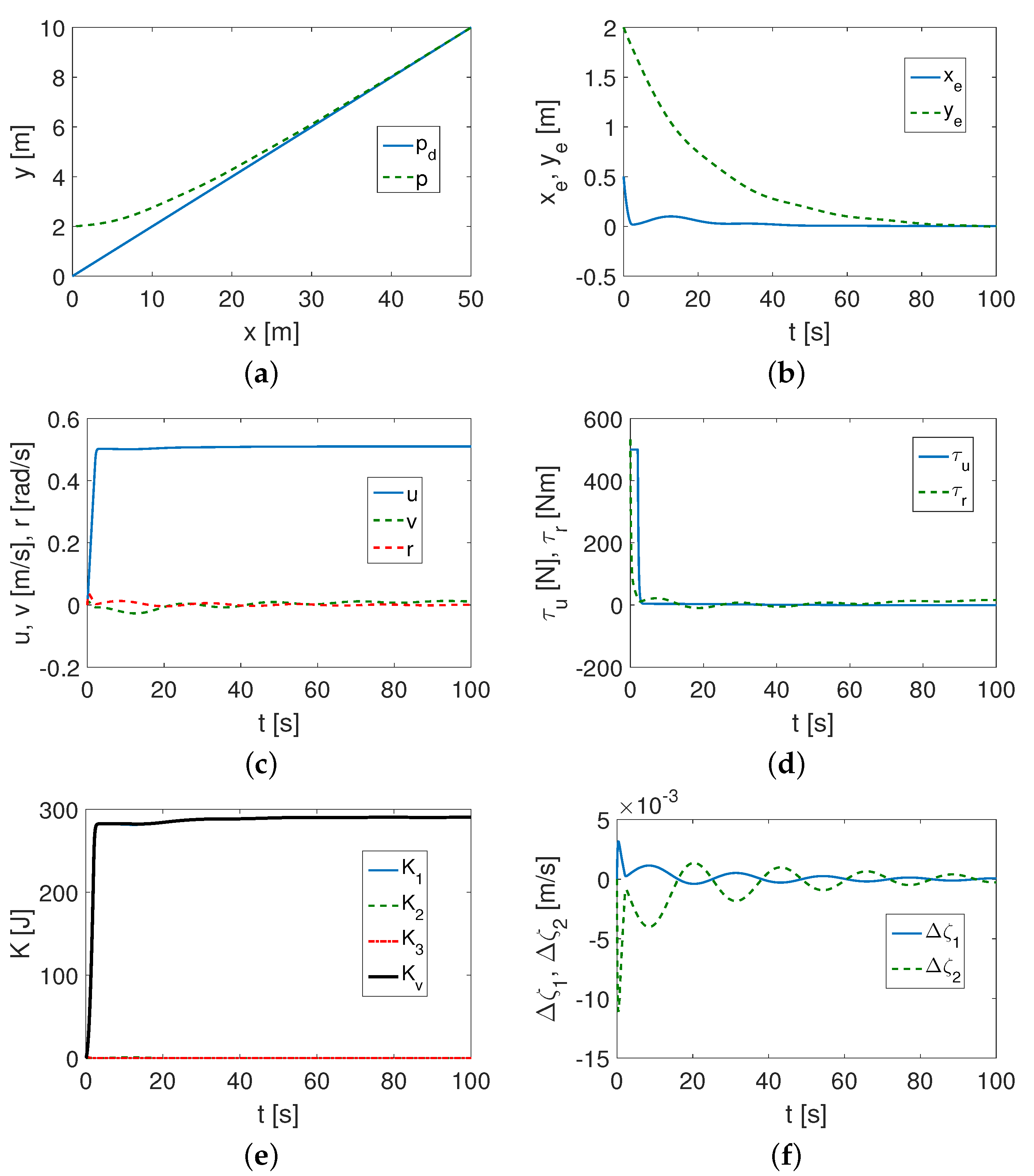
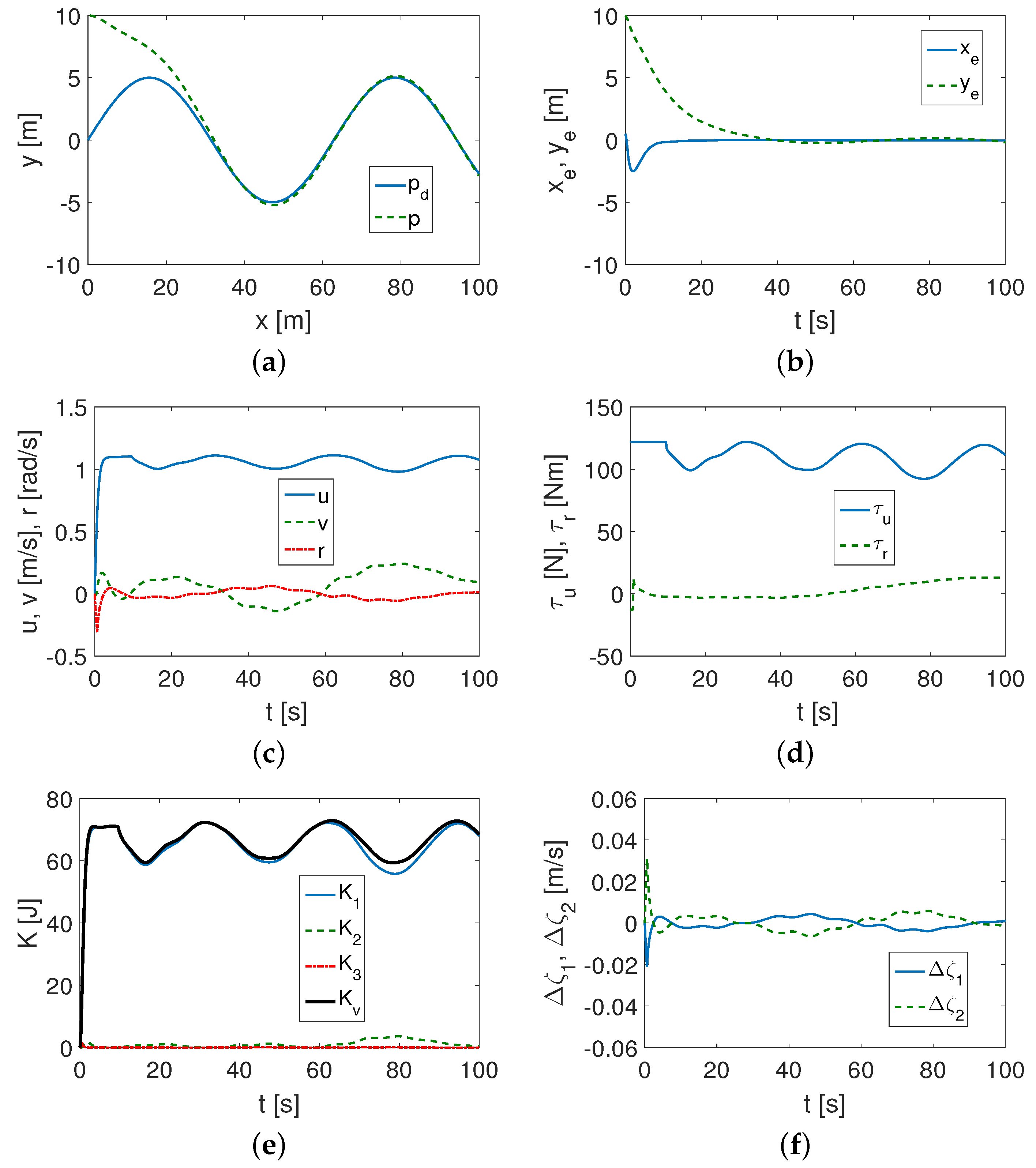
4.1.1. SIRENE Vehicle Test

Sine trajectory (58): The selected controller gains, to ensure acceptable error convergence, were as follows:

$$\begin{array}{ccc}\hfill & & k_1=0.05,k_2=0.25,k_3=10,k_4=2.0,k_5=10.\hfill \end{array}$$

(62)

As can be seen from Figure 3a, the task of trajectory tracking was carried out correctly, and the tracking errors tended to the final value, as confirmed in Figure 3b. Therefore, the controller was working correctly. From the speeds shown in Figure 3c, it is clear that the forward movement of the vehicle was dominant, although the lateral movement was also noticeable. The values of the force and torque (Figure 3d) reached the maximum values only in the first phase of movement (reaching the desired trajectory). The highest values of the kinetic energy correspond to the longitudinal velocity, as can be seen from Figure 3e. The mean kinetic energy values for quasi-velocity were as follows: $\delta K_1=1240.1$ J, $\delta K_2=37.6$ J, and $\delta K_3=3.2$ J. From the quasi-velocity errors shown in Figure 3f, the deformation of the longitudinal velocity due to the vehicle’s lack of symmetry was small, while the transverse velocity was slightly larger.

Linear trajectory (59): The gains to ensure acceptable error convergence were taken as follows:

$$\begin{array}{ccc}\hfill & & k_1=0.08,k_2=0.05,k_3=5.0,k_4=0.5,k_5=5.0.\hfill \end{array}$$

(63)

From Figure 4a,b, it can be seen that the task of trajectory tracking was realized, but for the errors of the uncontrollable variable, the time to reach the trajectory was long (about 80 s). The task was accomplished primarily by means of the longitudinal velocity u, which is observed in Figure 4c. Large values of the force ${\tau }_u$ and torque ${\tau }_r$ occurred only for a short time at the beginning of the vehicle movement (Figure 4d). The kinetic energy required to track a linear desired trajectory was much less than for tracking a sinus trajectory, as can be observed from Figure 4e. The mean kinetic energy values for the quasi-velocity were as follows: $\delta K_1=283.63$ J, $\delta K_2=0.15$ J, and $\delta K_3=0.02$ J. The velocities were only very slightly deformed, as indicated by the errors $\Delta {\zeta }_1,\Delta {\zeta }_2$ in Figure 4f.

Partial circle trajectory (60): In this case, the controller gains were selected as follows:

$$\begin{array}{ccc}\hfill & & k_1=0.04,k_2=0.30,k_3=2.5,k_4=3.5,k_5=10.\hfill \end{array}$$

(64)

As can be seen in Figure 5a,b, the circular trajectory was tracked correctly, although it was only after a few tens of seconds that the errors decreased significantly. Furthermore, with this kind of movement, the velocity u was dominant, but also the velocity v was important, as can be seen from Figure 5c. In the initial phase of the movement, signals ${\tau }_u,{\tau }_r$ reached maximum values, but after a short time, they decreased considerably (Figure 5d). The kinetic energy consumption was only slightly higher than with linear trajectory tracking, as illustrated in Figure 5e, but the velocity deformation was higher and similar to that for the sine trajectory, as indicated by the error values $\Delta {\zeta }_1,\Delta {\zeta }_2$ shown in Figure 5f. The mean kinetic energy values for quasi-velocity were as follows: $\delta K_1=266.22$ J, $\delta K_2=35.35$ J, and $\delta K_3=4.50$ J.

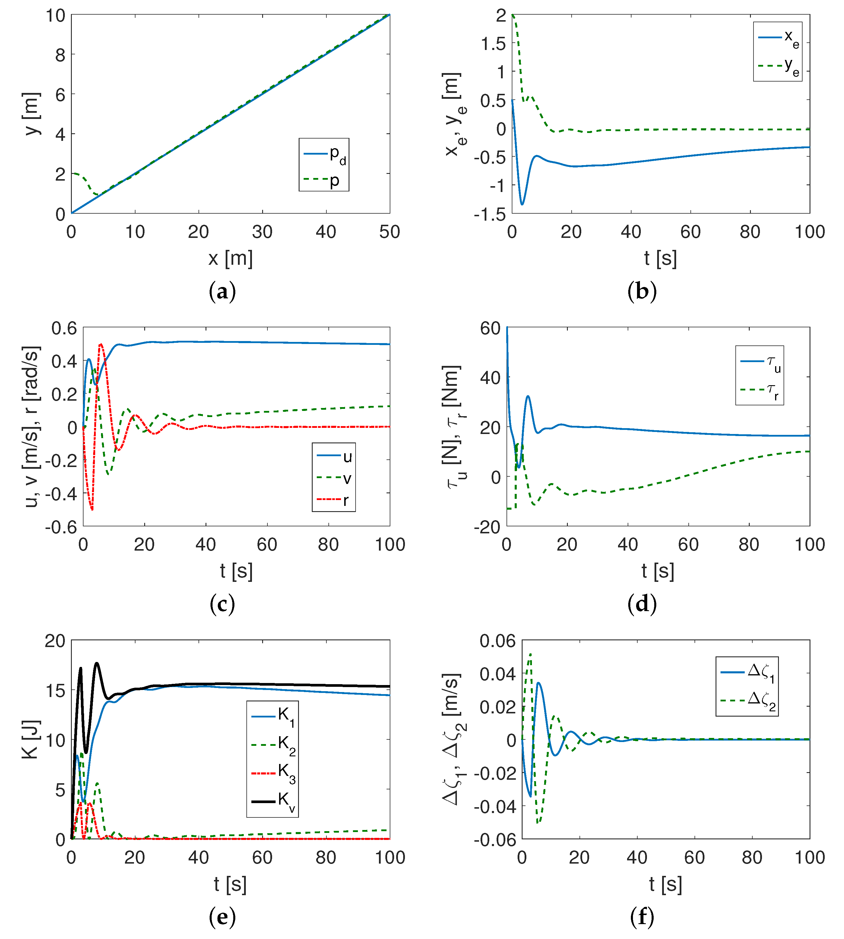
4.1.2. CETUS II Vehicle Test

The results presented in Figure 6a,b show that the sine trajectory tracking was performed with satisfactory accuracy. The velocity values in Figure 6c indicate that the movement was mainly due to the velocity u, although the lateral velocity v also had a visible contribution to the vehicle movement. The movement of the vehicle was primarily due to the $ta{u}_r$ force (unlike for the SIRENE vehicle), which only initially reached a maximum value, as shown in Figure 6d. The kinetic energy consumption (Figure 6e) also related primarily to the forward motion of the vehicle, which was consistent with the velocity history u. The mean kinetic energy values for the quasi-velocity were as follows: $\delta K_1=65.00$ J, $\delta K_2=1.08$ J, and $\delta K_3=0.02$ J. Figure 6f shows (errors $\Delta {\zeta }_1,\Delta {\zeta }_2$) that the velocity deformation due to the dynamic parameters of the applied model was not significant.

Sine trajectory (58): The selected controller gains, to ensure acceptable error convergence, were as follows:

$$\begin{array}{ccc}\hfill & & k_1=0.85,k_2=0.10,k_3=15,k_4=1.0,k_5=20.\hfill \end{array}$$

(65)

Linear trajectory (59): The selected controller gains, to ensure acceptable error convergence, were as follows:

$$\begin{array}{ccc}\hfill & & k_1=0.15,k_2=0.40,k_3=1.4,k_4=1.4,k_5=15.\hfill \end{array}$$

(66)

As can be seen in Figure 7a,b, the linear trajectory was tracked, but inaccurately, as evidenced by the $x_e$ error values. In addition, at the beginning, the movement of the CETUS vehicle was different from that of the SIRENE. This may be due to the less favorable mass-to-power ratio of the engines (the mass of the vehicle is small, and the propulsion capabilities are strongly limited). In Figure 7c, it can be observed that the dominant speed was u, but when the vehicle started, there were oscillations of the other velocities, which caused its irregular movement. Control signals ${\tau }_u$ and ${\tau }_r$ had maximum values only when the vehicle started and then significantly decreased, as shown in Figure 7d. Figure 7e indicates that the forward motion absorbed the most kinetic energy, but not as much as the motion along a sine trajectory. Energy oscillations in the initial phase of motion were caused by changes in the vehicle velocity. The mean kinetic energy values for quasi-velocity were as follows: $\delta K_1=14.18$ J, $\delta K_2=0.75$ J, and $\delta K_3=0.18$ J. The velocity disturbance was also reflected in the error histories $\Delta {\zeta }_1,\Delta {\zeta }_2$, as depicted in Figure 7f.

Partial circle trajectory (60): The controller gains, selected to ensure acceptable error convergence, were assumed as follows:

$$\begin{array}{ccc}\hfill & & k_1=0.15,k_2=0.40,k_3=2.0,k_4=15,k_5=15.\hfill \end{array}$$

(67)

From Figure 8a,b, it can be noted that the task of tracking a circular trajectory was indeed carried out, but as can be seen from Figure 2, the limitation of the $y_e$ error at the set time was quite high. The vehicle was not able to obtain a more accurate position error at this time. However, in this case, the velocity values settled after about 15 s, and the velocity u had the highest value, although the velocity v was also important for the movement of the vehicle, as can be deduced from Figure 8c. The force and torque values ${\tau }_u$ and ${\tau }_r$ were large only at the beginning of the movement (Figure 8d). The kinetic energy was reduced primarily by the forward motion of the vehicle, and its values were slightly higher than when implementing a linear trajectory, as can be viewed in Figure 8e. The mean kinetic energy values for the quasi-velocity were as follows: $\delta K_1=13.62$ J, $\delta K_2=1.90$ J, and $\delta K_3=0.08$ J. In the case under consideration, the velocity deformation errors $\Delta {\zeta }_1,\Delta {\zeta }_2$ shown in Figure 8f were larger than before.

The performance of the controller for the tested vehicles and trajectories is summarized in

Table 2. Performance for the SIRENE and CETUS II.

			SIRENE			CETUS II
Index		Sine t.	Linear t.	Circle t.	Sine t.	Linear t.	Circle t.
MIA	$x_e$	1.0393	0.0267	0.5562	0.1394	0.5334	0.4463
	$y_e$	0.6591	0.4005	0.1612	1.1292	0.1120	0.1435
MIAC	${\tau }_u$	74.539	12.498	35.537	110.29	18.238	17.822
	${\tau }_r$	156.02	10.326	204.72	5.2947	5.8960	5.3220
RMS	$||e||$	2.5771	0.6379	0.9426	2.4545	0.6439	0.7073
MKE	$\delta K$	1280.8	283.80	306.07	66.103	15.106	15.603
MQV	$\delta z$	1.2499	0.5144	0.7179	1.2000	0.6266	0.7191
MQVE	$\delta \Delta z$	0.0188	0.0013	0.0259	0.0051	0.0070	0.0108
CEI	$\delta \widehat{\Pi }$	1.3258	1.3258	1.3258	1.1232	1.1232	1.1232

.

The relative performances for the SIRENE and CETUS II are given in

Table 3. Relative performance for the SIRENE and CETUS II and for different trajectories.

			SIRENE			CETUS II
Index		Sine t.	Linear t.	Circle t.	Sine t.	Linear t.	Circle t.
MIA	$x_e$	100%	100%	100%	10.0%	1998%	80.2%
	$y_e$	100%	100%	100%	171%	28.0%	89.0%
MIAC	${\tau }_u$	59.6%	100%	284%	605%	100%	97.7%
	${\tau }_r$	1511%	100%	1983%	89.8%	100%	90.3%
RMS	$||e||$	100%	100%	100%	95.2%	101%	75.0%
MKE	$\delta K$	451%	100%	108%	476%	100%	103%
MQV	$\delta z$	100%	100%	100%	96.0%	122%	100%
MQVE	$\delta \Delta z$	100%	100%	100%	27.1%	538%	41.7%
CEI	$\delta \widehat{\Pi }$	100%	100%	100%	84.7%	84.7%	84.7%

. The quantities $x_e$, $y_e$, $||e||$, $\delta z$, and $\delta \Delta z$ refer to the selected vehicle and the corresponding trajectory (assumed 100% for the SIRENE and each of the trajectories tracked by this vehicle). The input signals ${\tau }_u$ and ${\tau }_r$ and the kinetic energy $\delta K$ concern each vehicle and the realized trajectory (it was assumed separately for the SIRENE and CETUS as 100 % when the linear trajectory was tracked as the simplest). The index $\delta \widehat{\Pi }$ indicates the couplings in the vehicle (for the SIRENE, it was assumed to be 100%).

4.2. Discussion of Results

The results of the simulation tests related only to the presented method. One objective was to test the effectiveness of the control scheme for different vehicles and other dynamic parameters and for the selected trajectories. A second objective, no less important, was to quantify the effect of mechanical couplings due to vehicle asymmetry on the vehicle’s motion after the proposed controller was applied.

As an example, models of two vehicles moving horizontally with distinctly different dynamic parameters were examined. The tests were realized for three types of desired trajectories, sine, line, and circular, assuming a limited tracking time of 100 seconds and taking into account the capabilities of the drives. The results obtained can be summarized as follows:

(1)

It was found that the performance of the proposed control algorithm was affected by both the vehicle dynamics and the selection of the desired trajectory.

(2)

If the vehicle had a large mass and the motors provided large force and force torque values (SIRENE), then the proposed algorithm was effective even in a limited time, and the performance was better than for a light vehicle (CETUS II) with small propulsion capabilities (force and force torques obtained).

(3)

All controller gain values were relevant to the tracking task to achieve acceptable performance. The most sensitive appeared to be $k_1$ and $k_2$, which were responsible for reducing the position error values. However, other gains, i.e., $k_3$, $k_4$, and $k_5$, also affected the control performance. Controller tuning was more effective for the SIRENE vehicle.

(4)

The test showed that the controller’s performance and tracking accuracy depended on the vehicle dynamics, the vehicle’s propulsion capabilities, and the selection of the desired trajectory. Furthermore, the control signals had the largest values for the sine trajectory.

(5)

It turned out that, in some cases, the algorithm was somehow robust to changes in the appropriately selected set of control gains, that is similar gain values could be applied to different trajectories.

(6)

The simulation studies demonstrated the suitability of the proposed algorithm both for control applications and for testing the dynamics of marine vehicles. Using the proposed control scheme, information was obtained that provided additional insight into the vehicle dynamics.

(a)

It was possible to analyze the kinetic energy corresponding to each IQV (and indirectly to velocity). The tests showed that the kinetic energy consumption depended not only on the parameters of the vehicle, but also on the trajectory to be followed. It turned out that the most kinetic energy was consumed by tracking a sine trajectory, and for other trajectories, it was much less.

(b)

The velocity deformation caused by the effect of vehicle asymmetry can be evaluated using indexes $\delta z$ and $\delta \Delta z$.

(c)

It was feasible to estimate the couplings in the vehicle model using the $\delta \widehat{\Pi }$ index because it reflected the parameters concerning the asymmetry of the inertia matrix.

(d)

A conclusion about the convergence of the errors on the basis of the indexes alone (MIA, RMS) can be misleading because they do not take into account the run history of these quantities. It is only by combining the index values with the error history that the performance of the controller can be reasonably deduced.

(e)

The effort associated with the ${\tau }_r$ control signal had large values compared to the ${\tau }_u$ signal for the SIRENE vehicle, while for the CETUS vehicle, the main effort came from the ${\tau }_u$ signal. This may be the reason that the control accuracy for the SIRENE was better.

Comment: This paper did not attempt to compare the proposed control algorithm with other algorithms in terms of performance. The first reason was that the presented scheme was used not only to guarantee trajectory tracking, but also to obtain information about the effect of couplings in the moving vehicle model. Of course, this approach was used, but for vehicles with all control signals available, as mentioned in the Introduction. For underactuated vehicles, this is rather uncommon with a few exceptions. The second reason was to verify the performance of the controller for vehicles with different parameters because verification on a single model may not be sufficient, as also stated in one of the papers cited in the Introduction. Here, two vehicles and three different trajectories were selected for testing. Therefore, the work was all about taking into account the change in the model and executed task. The third reason stemmed from the fact that the control scheme can be used for vehicles with full asymmetry (in two planes). Usually, however, either full symmetry (the center of mass coincides with the geometric center) or symmetry in one plane is assumed.

Remark 2.

The effectiveness of the control algorithm was based on the proper tuning of its parameters. However, even when this condition is met, other control strategies known from the literature may lead to better results (e.g., trajectory tracking accuracy) than the proposed controller. From the cited literature, it appears that performance improvements can be obtained by combinations of different approaches either adding observers or using neural networks. The proposed approach was based on classical control methods and also included the limitations of these methods. On the other hand, the added values are a generalization of the controller to a fully asymmetric model and obtaining information on the effect of couplings on vehicle movement.

The disadvantages and limitations of the proposed regulatorcan be stated as follows:

• The control scheme consisted of a kinematic algorithm and a dynamic algorithm. The use of each guaranteed only limited convergence to equilibrium. This caused position errors to add up and accuracy to seek some limit. While it can be reduced, it cannot be eliminated. This is due to the mathematical approach used.
• The dynamic and geometric parameters of the model had a significant impact on the performance of the controller. As a result, the force and torque had large values, especially when the vehicle started to move. In a real vehicle, such values may be impossible to achieve and, therefore, need to be limited to acceptable values (which is due to mechanical restrictions). This was performed in the conducted tests so that the realized trajectories did not exceed the values resulting from the drives of each tested vehicle, and at the same time, the conditions of the mathematical proof were met.
• The parameters of the kinematic controller $k_1$ and $k_2$ were sensitive to changes, and their increase led to oscillations; therefore, they must have limited values, which led to an increase in the time to achieve the desired trajectory. The selection of these gains is difficult because there is no side signal forcing. The changes in parameters relating to the dynamic part of the scheme $k_3$, $k_4$, and $k_5$ were also related to each other, which made their selection difficult (especially k4, because it relates to rotation and indirectly affects the lateral movement of the vehicle). In addition, some of the dynamic parameters affected changes in the desired virtual controls (i.e., $u_d$ and ${\mu }_d$).
• The performance of the controller was limited by the need to simultaneously meet the parameter selection conditions of the kinematic and dynamic controllers, as well as the requirements of the force and torque limitation.

Advantages of the proposed control method: The value of the considered approach to the trajectory tracking problem can be pointed out as follows:

• First, compared to control strategies based on a vehicle model with a diagonal inertia matrix (the assumption of full vehicle symmetry), the proposed algorithm is more general because it allows the use of a vehicle model that is asymmetric in two planes. This distinguishes the presented algorithm from others that are suitable for vehicle models without inertial coupling, e.g., [8,9,24,58], and additionally oriented toward improving performance against a known control scheme [26]. Even controllers suitable for an asymmetric model [31,33,36] cannot be considered suitable for the general case (with full asymmetry).
• Second, the use of velocity transformation allowed the controller to apply dynamic equations with a diagonal inertia matrix. An important advantage is that the information contained in the original nonlinear model remains in the diagonalized equations, which makes it possible to incorporate them into the control algorithm.
• Third, using the offered control scheme, it is possible to estimate the effect of couplings during the realization of the trajectory tracking task, something that algorithms oriented only toward performance improvement do not provide. This property of the proposed algorithm gives the advantage that, without performing an experiment on a real vehicle, it is possible to determine whether the couplings are significant in the vehicle model or can be neglected.

5. Conclusions

This paper developed a nonlinear tracking control algorithm for underactuated marine vehicles to resist unknown internal and external disturbances. An important property of this algorithm is that it is not only suitable for the tracking task, but also provides some insight into the behavior of an asymmetric vehicle during trajectory tracking. This is possible through the use of classical methods such as backstepping and SMC, but provided that the description of the dynamics in quasi-velocities resulting from the decomposition of the inertia matrix is employed. From a theoretical point of view, the proposed algorithm guarantees uniformly ultimately boundedness, but it also makes it possible to evaluate the vehicle’s behavior when tracking a desired trajectory already at the stage of preliminary studies (without realizing the real experiment). This was performed by making assumptions due to the technical constraints, analyzing the signal obtained in the simulation studies, and analyzing a selected set of indexes. In order to demonstrate the suitability of the control scheme, simulation tests were performed for a model of two vehicles with significantly different dynamics, three selected trajectories, and propulsion limitations, which demonstrated the effectiveness of the method and allowed the discussion of the results produced. The proposed control scheme was verified by simulations on real vehicle models used in practice. Graphical results were presented, as well as some quantitative results obtained based on the assumed measures. The discussion of the results pointed out the advantages, disadvantages, and limitations of the applicability of the proposed control method. In the future, other types of algorithms based on diagonalized equations of motion should be studied. The verification of these types of algorithms on models of other real and designed vehicles is also planned. The proposed approach also needs to be tested on vehicles moving in three-dimensional space.

References

1. Jiang, Z.P. Global tracking control of underactuated ships by Lyapunov’s direct method. Automatica 2002, 38, 301–309. [Google Scholar] [CrossRef]
2. Lefeber, E.; Pettersen, K.Y.; Nijmeijer, H. Tracking Control of an Underactuated Ship. IEEE Trans. Control. Syst. Technol. 2003, 11, 52–61. [Google Scholar] [CrossRef] [Green Version]
3. Godhavn, J.M. Nonlinear tracking of underactuated surface vessels. In Proceedings of the 35th IEEE Conference on Decision and Control, Kobe, Japan, 11–13 December 1996; pp. 975–980. [Google Scholar]
4. Repoulias, F.; Papadopoulos, E. Planar trajectory planning and tracking control design for underactuated AUVs. Ocean Eng. 2007, 34, 1650–1667. [Google Scholar] [CrossRef]
5. Do, K.D. Robust adaptive tracking control of underactuated ODINs under stochastic sea loads. Robot. Auton. Syst. 2015, 72, 152–163. [Google Scholar] [CrossRef]
6. Sun, Z.; Zhang, G.; Qiao, L.; Zhang, W. Robust adaptive trajectory tracking control of underactuated surface vessel in fields of marine practice. J. Mar. Sci. Technol. 2018, 23, 950–957. [Google Scholar] [CrossRef]
7. Zhao, Y.; Sun, X.; Wang, G.; Fan, Y. Adaptive Backstepping Sliding Mode Tracking Control for Underactuated Unmanned Surface Vehicle With Disturbances and Input Saturation. IEEE Access 2021, 9, 1304–1312. [Google Scholar] [CrossRef]
8. Elmokadem, T.; Zribi, M.; Youcef-Toumi, K. Trajectory tracking sliding mode control of underactuated AUVs. Nonlinear Dyn. 2016, 84, 1079–1091. [Google Scholar] [CrossRef] [Green Version]
9. Zhang, L.; Huang, B.; Liao, Y.; Wang, B. Finite-Time Trajectory Tracking Control for Uncertain Underactuated Marine Surface Vessels. IEEE Access 2019, 7, 102321–102330. [Google Scholar] [CrossRef]
10. Elmokadem, T.; Zribi, M.; Youcef-Toumi, K. Terminal sliding mode control for the trajectory tracking of underactuated Autonomous Underwater Vehicles. Ocean Eng. 2017, 129, 613–625. [Google Scholar] [CrossRef]
11. Sun, Y.; Chai, P.; Zhang, G.; Zhou, T.; Zheng, H. Sliding Mode Motion Control AUV Dual-Obs. Thruster Uncertainty. J. Mar. Sci. Eng. 2022, 10, 349. [Google Scholar] [CrossRef]
12. Vu, M.T.; Le, T.H.; Thanh, H.L.N.N.; Huynh, T.T.; Van, M.; Hoang, Q.D.; Do, T.D. Robust Position Control of an Over-actuated Underwater Vehicle under Model Uncertainties and Ocean Current Effects Using Dynamic Sliding Mode Surface and Optimal Allocation Control. Sensors 2021, 21, 747. [Google Scholar] [CrossRef]
13. Vu, M.T.; Thanh, H.L.N.N.; Huynh, T.T.; Do, Q.T.; Do, T.D.; Hoang, Q.D.; Le, T.H. Station-Keeping Control of a Hovering Over-Actuated Autonomous Underwater Vehicle Under Ocean Current Effects and Model Uncertainties in Horizontal Plane. IEEE Access 2021, 9, 6855–6867. [Google Scholar] [CrossRef]
14. Tijjani, A.S.; Chemori, A.; Creuze, V. Robust Adaptive Tracking Control of Underwater Vehicles: Design, Stability Analysis, and Experiments. IEEE/ASME Trans. Mechatr. 2021, 26, 897–907. [Google Scholar] [CrossRef]
15. Alattas, K.A.; Mobayen, S.; Din, S.U.; Asad, J.H.; Fekih, A.; Assawinchaichote, W.; Vu, M.T. Design of a Non-Singular Adaptive Integral-Type Finite Time Tracking Control for Nonlinear Systems With External Disturbances. IEEE Access 2021, 9, 102091–102103. [Google Scholar] [CrossRef]
16. Osler, S.; Sands, T. Controlling Remotely Operated Vehicles with Deterministic Artificial Intelligence. Appl. Sci. 2022, 12, 2810. [Google Scholar] [CrossRef]
17. Sands, T. Development of Deterministic Artificial Intelligence for Unmanned Underwater Vehicles (UUV). J. Mar. Sci. Eng. 2020, 8, 578. [Google Scholar] [CrossRef]
18. Shah, R.; Sands, T. Comparing Methods of DC Motor Control for UUVs. Appl. Sci. 2021, 11, 4972. [Google Scholar] [CrossRef]
19. Sands, T. Control of DC Motors to Guide Unmanned Underwater Vehicles. Appl. Sci. 2021, 11, 2144. [Google Scholar] [CrossRef]
20. Koo, S.M.; Travis, H.; Sands, T. Impacts of Discretization and Numerical Propagation on the Ability to Follow Challenging Square Wave Commands. J. Mar. Sci. Eng. 2022, 10, 419. [Google Scholar] [CrossRef]
21. Zhai, H.; Sands, T. Controlling Chaos in Van Der Pol Dynamics Using Signal-Encoded Deep Learning. Mathematics 2022, 10, 453. [Google Scholar] [CrossRef]
22. Zhai, H.; Sands, T. Comparison of Deep Learning and Deterministic Algorithms for Control Modeling. Sensors 2022, 22, 6362. [Google Scholar] [CrossRef] [PubMed]
23. Pan, C.Z.; Lai, X.Z.; Wang, S.X.; Wu, M. An efficient neural network approach to tracking control of an autonomous surface vehicle with unknown dynamics. Expert Syst. Appl. 2013, 40, 1629–1635. [Google Scholar] [CrossRef]
24. Zhang, C.; Wang, C.; Wei, Y.; Wang, J. Neural-Based Command Filtered Backstepping Control for Trajectory Tracking of Underactuated Autonomous Surface Vehicles. IEEE Access 2020, 8, 42482–42490. [Google Scholar] [CrossRef]
25. Zhang, L.J.; Qi, X.; Pang, Y.J. Adaptive output feedback control based on DRFNN for AUV. Ocean Eng. 2009, 36, 716–722. [Google Scholar] [CrossRef]
26. Zhu, G.; Ma, Y.; Li, Z.; Malekian, R.; Sotelo, M. Event-Triggered Adaptive Neural Fault-Tolerant Control of Underactuated MSVs With Input Saturation. IEEE Trans. Intell. Transp. Syst. 2022, 23, 7045–7057. [Google Scholar] [CrossRef]
27. Duan, K.; Fong, S.; Chen, P. Fuzzy observer-based tracking control of an underactuated underwater vehicle with linear velocity estimation. IET Control. Theory Appl. 2020, 14, 584–593. [Google Scholar] [CrossRef]
28. Li, J.; Du, J.; Sun, Y.; Lewis, F.L. Robust adaptive trajectory tracking control of underactuated autonomous underwater vehicles with prescribed performance. Int. J. Robust Nonlinear Control 2019, 29, 4629–4643. [Google Scholar] [CrossRef]
29. Dong, Z.; Wan, L.; Liu, T.; Zeng, J. Horizontal-plane Trajectory-tracking Control of an Underactuated Unmanned Marine Vehicle in the Presence of Ocean Currents. Int. J. Adv. Robot. Syst. 2016, 13, 63634. [Google Scholar] [CrossRef] [Green Version]
30. Zhang, Z.; Wu, Y. Further results on global stabilisation and tracking control for underactuated surface vessels with non-diagonal inertia and damping matrices. Int. J. Control. 2015, 88, 1679–1692. [Google Scholar] [CrossRef]
31. Wang, C.; Xie, S.; Chen, H.; Peng, Y.; Zhang, D. A decoupling controller by hierarchical backstepping method for straight-line tracking of unmanned surface vehicle. Syst. Sci. Control. Eng. 2019, 7, 379–388. [Google Scholar] [CrossRef]
32. Wang, N.; Xie, G.; Pan, X.; Su, S.F. Full-State Regulation Control of Asymmetric Underactuated Surface Vehicles. IEEE Trans. Ind. Electron. 2019, 66, 8741–8750. [Google Scholar] [CrossRef]
33. Chen, L.; Cui, R.; Yang, C.; Yan, W. Adaptive Neural Network Control of Underactuated Surface Vessels with Guaranteed Transient Performance: Theory and Experimental Results. IEEE Trans. Ind. Electron. 2020, 67, 4024–4035. [Google Scholar] [CrossRef] [Green Version]
34. Park, B.S. Neural Network-Based Tracking Control of Underactuated Autonomous Underwater Vehicles With Model Uncertainties. J. Dyn. Syst. Meas. Control. Trans. ASME 2015, 137, 021004. [Google Scholar] [CrossRef]
35. Dai, S.L.; He, S.; Lin, H. Transverse function control with prescribed performance guarantees for underactuated marine surface vehicles. Int. J. Robust Nonlinear Control 2019, 29, 1577–1596. [Google Scholar] [CrossRef]
36. Qiu, B.; Wang, G.; Fan, Y.; Mu, D.; Sun, X. Adaptive Sliding Mode Trajectory Tracking Control for Unmanned Surface Vehicle with Modeling Uncertainties and Input Saturation. Appl. Sci. 2019, 9, 1240. [Google Scholar] [CrossRef] [Green Version]
37. Ashrafiuon, H.; Nersesov, S.; Clayton, G. Trajectory Tracking Control of Planar Underactuated Vehicles. IEEE Trans. Autom. Control. 2017, 62, 1959–1965. [Google Scholar] [CrossRef]
38. Xia, Y.; Xu, K.; Li, Y.; Xu, G.; Xiang, X. Improved line-of-sight trajectory tracking control of under-actuated AUV subjects to ocean currents and input saturation. Ocean Eng. 2019, 174, 14–30. [Google Scholar] [CrossRef]
39. Park, B.S.; Yoo, J.Y. Robust trajectory tracking with adjustable performance of underactuated surface vessels via quantized state feedback. Ocean Eng. 2022, 246, 110475. [Google Scholar] [CrossRef]
40. Jia, Z.; Hu, Z.; Zhang, W. Adaptive output-feedback control with prescribed performance for trajectory tracking of underactuated surface vessels. ISA Trans. 2019, 95, 18–26. [Google Scholar] [CrossRef]
41. Paliotta, C.; Lefeber, E.; Pettersen, K.Y.; Pinto, J.; Costa, M.; de Figueiredo Borges de Sousa, J.T. Trajectory Tracking and Path Following for Underactuated Marine Vehicles. IEEE Trans. Control. Syst. Technol. 2019, 27, 1423–1437. [Google Scholar] [CrossRef] [Green Version]
42. Wang, N.; Su, S.F. Finite-Time Unknown Observer-Based Interactive Trajectory Tracking Control of Asymmetric Underactuated Surface Vehicles. IEEE Trans. Control. Syst. Technol. 2014, 29, 794–803. [Google Scholar] [CrossRef]
43. Herman, P. Numerical Test of Several Controllers for Underactuated Underwater Vehicles. Appl. Sci. 2020, 10, 8292. [Google Scholar] [CrossRef]
44. Kozlowski, K.; Herman, P. Control of Robot Manipulators in Terms of Quasi-Velocities. J. Intell. Robot. Syst. 2008, 53, 205–221. [Google Scholar] [CrossRef]
45. Sinclair, A.J.; Hurtado, J.E.; Junkins, J.L. Linear Feedback Controls using Quasi Velocities. J. Guid. Control. Dyn. 2006, 29, 1309–1314. [Google Scholar] [CrossRef] [Green Version]
46. Herman, P. Application of nonlinear controller for dynamics evaluation of underwater vehicles. Ocean Eng. 2019, 179, 59–66. [Google Scholar] [CrossRef]
47. Herman, P. Vehicle Dynamics Study Based on Nonlinear Controllers Conclusions and Perspectives. In Inertial Quasi-Velocity Based Controllers for a Class of Vehicles; Springer Tracts in Mechanical Engineering; Springer: Cham, Switzerland, 2022. [Google Scholar] [CrossRef]
48. Li, S.; Wan, X.; Zhang, L. Finite-Time Output Feedback Tracking Control for Autonomous Underwater Vehicles. IEEE J. Ocean. Eng. 2015, 40, 727–751. [Google Scholar] [CrossRef]
49. Yan, Z.; Wang, M.; Xu, J. Robust adaptive sliding mode control of underactuated autonomous underwater vehicles with uncertain dynamics. Ocean Eng. 2019, 173, 802–809. [Google Scholar] [CrossRef]
50. Fossen, T.I. Guidance and Control of Ocean Vehicles; John Wiley and Sons: Chichester, UK, 1994. [Google Scholar]
51. Loduha, T.A.; Ravani, B. On First-Order Decoupling of Equations of Motion for Constrained Dynamical Systems. Trans. ASME J. Appl. Mech. 1995, 62, 216–222. [Google Scholar] [CrossRef]
52. Vu, M.T.; Van, M.; Bui, D.H.P.; Do, Q.T.; Huynh, T.T.; Lee, S.D.; Choi, H.S. Study on Dynamic Behavior of Unmanned Surface Vehicle-Linked Unmanned Underwater Vehicle System for Underwater Exploration. Sensors 2020, 20, 1329. [Google Scholar] [CrossRef] [Green Version]
53. Peng, Z.; Wang, J.; Han, Q.L. Path-Following Control of Autonomous Underwater Vehicles Subject to Velocity and Input Constraints via Neurodynamic Optimization. IEEE Trans. Ind. Electron. 2019, 66, 8724–8732. [Google Scholar] [CrossRef]
54. Yu, H.; Guo, C.; Yan, Z. Globally finite-time stable three-dimensional trajectory-tracking control of underactuated UUVs. Ocean Eng. 2019, 189, 106329. [Google Scholar] [CrossRef]
55. Qiao, L.; Zhang, W. Double-Loop Integral Terminal Sliding Mode Tracking Control for UUVs With Adaptive Dynamic Compensation of Uncertainties and Disturbances. IEEE J. Ocean. Eng. 2019, 44, 29–53. [Google Scholar] [CrossRef]
56. Fierro, R.; Lewis, F.L. Control of a nonholonomic mobile robot: Backsteping kinematics into dynamics. In Proceedings of the 34th IEEE conference on Decision and Control, New Orleans, LA, USA, 13–15 December 1995; pp. 3805–3810. [Google Scholar]
57. Fierro, R.; Lewis, F.L. Control of a Nonholonomic Mobile Robot: Backsteping Kinematics into Dynamics. J. Robot. Syst. 1997, 14, 149–163. [Google Scholar] [CrossRef]
58. Xu, J.; Wang, M.; Qiao, L. Dynamical sliding mode control for the trajectory tracking of underactuated unmanned underwater vehicles. Ocean Eng. 2015, 105, 54–63. [Google Scholar] [CrossRef]
59. Marczak, A. Software: Robust Adaptive Trajectory Tracking Control of Underactuated Surface Vessel in Fields of Marine Practice. Unpublished project. Poznan University of Technology, Poznań, Poland, 2022. [Google Scholar]
60. Batista, P.; Silvestre, C.; Oliveira, P. A two-step control approach for docking of autonomous underwater vehicles. Int. J. Robust Nonlinear Control 2015, 25, 1528–1547. [Google Scholar] [CrossRef]
61. Silvestre, C.; Aguiar, A.; Oliveira, P.; Pascoal, A. Control of the SIRENE underwater shuttle: System design and tests at sea. In Proceedings of the 17th International Conference on Offshore Mechanics and Arctic Engineering, Lisbon, Portugal, 5–9 July 1998. [Google Scholar]
62. Barisic, M.; Vasilijevic, A.; Nad, D. Sigma-Point Unscented Kalman Filter Used For AUV Navigation. In Proceedings of the 2012 20th Mediterranean Conference on Control & Automation (MED), Barcelona, Spain, 3–6 July 2012; pp. 1365–1372. [Google Scholar]
63. Djapic, V. Unifying Behavior Based Control Design and Hybrid Stability Theory for AUV Application. Ph.D. Thesis, University of California, Riverside, CA, USA, 2009. [Google Scholar]
Figure 1. Underwater vehicle model sketch.
Jmse 11 00509 g001
Figure 2. Proposed control scheme.
Jmse 11 00509 g002
Figure 3. Results for the SIRENE, QV controller and sine trajectory: (a) desired and realized trajectory; (b) position errors; (c) velocity errors; (d) applied force and torque; (e) kinetic energy time history; (f) quasi-velocity errors Δ ζ 1 , Δ ζ 2 .
Jmse 11 00509 g003
Figure 4. Results for the SIRENE, QV controller and linear trajectory: (a) desired and realized trajectory; (b) position errors; (c) velocity errors; (d) applied force and torque; (e) kinetic energy time history; (f) quasi-velocity errors Δ ζ 1 , Δ ζ 2 .
Jmse 11 00509 g004
Figure 5. Results for the SIRENE, QV controller and partial circular trajectory: (a) desired and realized trajectory; (b) position errors; (c) velocity errors; (d) applied force and torque; (e) kinetic energy time history; (f) quasi-velocity errors Δ ζ 1 , Δ ζ 2 .
Jmse 11 00509 g005
Figure 6. Results for the CETUS II, QV controller and sine trajectory: (a) desired and realized trajectory; (b) position errors; (c) velocity errors; (d) applied force and torque; (e) kinetic energy time history; (f) quasi-velocity errors Δ ζ 1 , Δ ζ 2 .
Jmse 11 00509 g006
Figure 7. Results for the CETUS II, QV controller and linear trajectory: (a) desired and realized trajectory; (b) position errors; (c) velocity errors; (d) applied force and torque; (e) kinetic energy time history; (f) quasi-velocity errors Δ ζ 1 , Δ ζ 2 .
Jmse 11 00509 g007
Figure 8. Results for the CETUS II, QV controller and partial circular trajectory: (a) desired and realized trajectory; (b) position errors; (c) velocity errors; (d) applied force and torque; (e) kinetic energy time history; (f) quasi-velocity errors Δ ζ 1 , Δ ζ 2 .
Jmse 11 00509 g008