Softening/Hardening Damage Model and Numerical Implementation of Seabed Silt-Steel Interface in Yellow River Underwater Delta

Abstract

The interaction between soil and structure is a research hotspot in ocean engineering, and the shear performance of interfaces is an essential factor affecting the bearing capacity of offshore structures. Taking the Yellow River Underwater Delta as the research area, the Softening/Hardening damage model of the silt–steel interface and the determination method of model parameters are proposed based on the statistical damage theory. Through the interface monotonic shear test under the conditions of different normal stress, roughness and water content, the shear mechanical properties and volumetric deformation laws on the silt–steel interface are analyzed, and the damage model parameters are obtained. Finally, a FRIC subroutine for the damage model was developed based on ABAQUS. The research results indicate the following: (1) The interface between silt and steel exhibits two characteristics, softening/hardening and shear shrinkage/expansion, under different conditions. Roughness significantly impacts interfacial cohesion, while water content mainly affects the internal friction angle. (2) The softening model based on the classic rock damage model can better simulate the stress–strain relationship of the silt–steel interface under high normal stress and low water content. In contrast, the hardening model based on the classic hyperbola model can better simulate the stress–strain relationship under low normal stress and high water content. The calculated results of the softening/hardening model agree with the experimental results, and the model has 7 parameters. (3) The developed FRIC subroutine can effectively simulate the nonlinear mechanical behavior of the interface between silt and steel. The research results provide a reference for exploring the stability analysis of offshore structures considering interface weakening effects.

1. Introduction

The ocean contains many mineral, oil and wind energy resources. In today’s global energy shortage and deteriorating ecological environment, ocean wind energy, as an emerging strategic resource, is increasingly valued by countries worldwide for its development and utilization [1]. China’s coastline is narrow and long, with abundant wind energy reserves that can be developed and utilized at sea. With the support of the “Ocean Power” and “Dual Carbon” policies, the development of marine wind power-related industries is rapid. In 2022, China’s offshore wind power increased its lifting capacity by 5.16 million kilowatts, accounting for approximately 54% of the global total. The cumulative lifting capacity was 30.51 million kilowatts, an increase of over 20% year-on-year, and it continues to maintain its position as the world’s largest [2].

The Yellow River Delta is rich in oil and gas resources and wind energy resources, and the mudflat and shallow sea areas are vast. Under the development strategy of “transformation of new and old kinetic energy”, several wind power bases in the south, north and Bohai Peninsula have been planned (Figure 1), with the planned installed capacity of 23.4 million kW, which will significantly promote the large-scale development of offshore wind power in the Yellow River Delta in the next few years [3]. In the shallow sea area of the Yellow River Delta, silty seabed soil is formed in the process of rapid sedimentation, pore water is not effectively discharged and surface sediment is not compacted, so it has the characteristics of high water content and low shear strength [4]. The construction of offshore wind power will change the seabed soil’s original stable environment and boundary conditions. Due to the multi-process coupling of complex dynamic loads and the interaction between structures and seabed soil, it is easy to induce the weakening of the soil–structure interface [5], which in turn leads to local/overall failure of the structural foundation, which will seriously affect the safety and stability of wind power foundations. Therefore, studying the mechanical properties of the soil and structural interface in the region is an urgent issue that needs to be addressed.

The constitutive interface model is used to describe the relationship between stress and strain during the shear process, analyze the mechanical properties of the interface and is of great significance for studying the interaction between soil and structure [6]. Three standard interface constitutive models exist: elastic, elastic-plastic and damage. Based on the elastic theory of generalized Hooke’s law, the hyperbola model has become one of the most popular interface constitutive models because of its few parameters, clear physical meaning, broad applicability to soil types and other advantages. Considering that the rigid plastic model or hyperbola model artificially assumes that the mutual displacement and shear stress in the interface contact zone conform to the inelastic or that nonlinear cannot fully fit the actual situation, many scholars combine the nonlinear elastic theory with the elastoplastic theory and propose the elastoplastic model of the soil–structure interface. Liu et al. (2014) [7] proposed a constitutive interface model based on critical state soil mechanics and generalized plasticity, which can simulate the monotonic and cyclic 3D behavior of soil–structure interfaces over a wide range of soil density, normal pressure and normal stiffness. Stutz et al. (2016) [8] proposed an enhanced non-plastic interface model that converts existing plastic models with predefined sand limit state surfaces into interface models by reducing stress and tension vectors and redefining tensors. Hosseinali and Toufigh (2018) [9] proposed a new plasticity-based constitutive model that can model strain-softening behavior in the tangential direction and shear expansion behavior in the normal direction. Saberi et al. (2020) [10] continuously revised and improved a two-sided plastic interface constitutive model by introducing factors such as critical state soil mechanics, particle breakage rate, new failure surfaces and 3D shear coupled loads, enabling the interface model to simulate complex behaviors of various soil–structure interfaces, such as stress hardening and softening, stress path dependence, phase transition, cyclic cumulative shrinkage and stability, stress degradation and particle breakage. Lu et al. (2017) [11] proposed a constitutive model for soil–structure interfaces by combining the tangential stress–strain relationship and normal stress–strain relationship of contact surface soils.

Damage mechanics is the rudiment of the discipline proposed by relevant scholars when studying the deformation and failure of metal materials. Subsequently, Ajcinovic and Silva (1982) [12] first proposed the concept of the “damage factor,” which laid the foundation for developing the constitutive model of damage mechanics. The so-called “damage”, the gradual creep evolution and ultimate failure of materials under loading is a branch of the solid mechanics of materials. In recent years, relevant scholars have made additional amendments based on metal damage mechanics in geotechnical engineering, considering that the rock and soil still bear part of the shear strength and hydrostatic pressure when damaged. They have developed rock and soil damage mechanics by viewing the mechanical properties of rock and soil and introducing stochastic statistical theory. Referring to the statistical model of damage evolution in rock mechanics, many scholars have also proposed a damage mechanics model suitable for soil-structure contact. Hu and Pu (2004) [13] proposed a damage constitutive model with ten parameters to describe the behavior of rough interfaces. Long et al. (2017) [14] proposed a damage model with only four parameters based on Weibull distribution statistical damage theory, which can effectively describe strain softening behavior. Zhao et al. (2017) [15] adopted the theory of damage mechanics based on the assumption of equal strain distribution, zero elastic region and no coupling of elastic strain and selected the ratio of irreversible volume strain to the maximum irreversible volume strain as the damage factor and established a shear strength and compressive volume strain damage model to describe the shear behavior of the interface between frozen soil and structure. Zhu and Guo (2016) [16] and Chen et al. (2022) [17] derived a constitutive model for frozen soil damage under dynamic loads based on deep learning, which can reflect the relationship between temperature and strain. Sun et al. (2020) [18] proposed an elastic-plastic damage constitutive model based on the overload/overload yield surface by observing the mechanical behavior of frozen sand and frozen saline soil in triaxial compression tests under different confining pressures. Liu et al. (2020) [19] introduced the concept of thermal damage and constructed a thermal damage model for rocks, expanding the research on rock strength theory. Rehman and Zhang (2021) [20] established a three-dimensional elastic-plastic damage model for gravel soil–structure interface considering the shear coupling effect. From this, it can be seen that the evolution of interface strength under shear is analogous to the damage process of metal materials. Assuming that the stress and strain at the interface conform to a specific statistical law based on the existing rock damage constitutive relationship, the damage mathematical model at this interface type is reasonable and feasible by modifying the shear test results.

Based on the research of relevant scholars on statistical damage theory, this paper proposes a softening/hardening damage model for the silt–steel interface in the Yellow River Delta. The model has 7 parameters and was obtained through large-scale interface shear tests. Finally, the rationality of the model is verified. At the same time, its application in the numerical calculation is realized, which is convenient for the subsequent numerical simulation research on the stability of offshore structures, considering the interface weakening effect, and is expected to guide the safety assessment of offshore installations in the Yellow River Delta.

2. Softening/Hardening Damage Model

2.1. Assumption

Numerous research results have shown that the soil–structure interface exhibits a strain-softening phenomenon during the shear process [21,22]. To derive the softening/hardening damage mathematical model applicable to the silt–steel interface in the Yellow River Delta and describe the two states of hardening and softening, this paper will combine the classic hyperbola model [23] and the classic rock damage model [14] to build.

According to damage mechanics and stochastic statistical theory, the following assumptions are set:

(1)

Assuming the soil is isotropic and the structure is a fixed rigid body.

(2)

Divide the soil–structure interface into several microelements, assuming that there are only two states: undamaged (0) and damaged (1).

(3)

Assuming that all friction and contact on the soil–structure interface (between soil particles, between soil structure) are unevenly and randomly distributed, the shear strength and shear failure at the interface are also unevenly and randomly distributed.

(4)

Assuming that the damage process at the soil–structure interface is a continuous process that undergoes an evolution from undamaged to damage, the soil at the interface can be divided into two parts, damaged soil and undamaged soil (Figure 2), and the undamaged soil bears effective stress.

2.2. Model Derivation

Based on the above assumptions, the damage process at the soil–structure interface satisfies the following relationship:

$$B=\frac{N_1}{N_2}\left(0\le B\le 1\right)$$

(1)

$$\tau N={\tau }_1{N}_1+{\tau }_2{N}_2$$

(2)

In the formula, B represents the degree of damage; τ₁ and τ₂ refer to the shear stress borne by damaged and undamaged soil, respectively.

Subsequently, Equation (2) can be transformed into the following form:

$$\tau ={\tau }_{1}B+{\tau }_2\left(1-B\right)$$

(3)

For undamaged soil N₂, the stress–strain relationship satisfies linear elasticity, and the shear stress is manifested as:

$${\tau }_2={\gamma }_2{G}_2$$

(4)

In the formula, γ₂ is the shear strain of undamaged soil; G₂ is the shear modulus of undamaged soil.

For the damaged soil N₁, when B approaches 1, τ trend τ₁. The damaged soil describes the mechanical characteristics of the overall interface failure.

Combined with the previous shear test results of silt in the Yellow River Delta [24], the hardening curve’s shear stress–strain curve conforms to the traditional hyperbola model; for the softening curve, there is residual friction strength after shear failure. Based on this, it is assumed that the shear stress of the damaged soil mass τ₁ satisfies the following equation:

$${\tau }_1=\{\begin{array}{c}\frac{{\tau }_1{G}_1}{{\gamma }_1\left(\frac{G_1}{\alpha }\right)+1}\hspace{1em}\mathrm{Hardening}\\ {\tau }_r \mathrm{Softening}\end{array}$$

(5)

In the formula, γ₁ is the shear strain of the damaged soil; G₁ is the shear modulus of the damaged soil; α is the hyperbola model parameter; τ_r is the residual shear stress.

Based on the assumption of equal strain, the following conditions are met:

$$\gamma ={\gamma }_1={\gamma }_2$$

(6)

From Equations (3)–(5), a mathematical model for the softening/hardening damage of the silt–steel interface is obtained:

$$\tau =\{\begin{array}{c}\frac{B\gamma G_1}{\gamma \left(\frac{G_1}{\alpha }\right)+1}+\left(1-B\right)\gamma G_2\hspace{1em}\mathrm{Hardening}\\ B{\tau }_r+\left(1-B\right)\gamma G_2 \mathrm{Softening}\end{array}$$

(7)

Assuming that the interface satisfies the Weibull distribution theory [25]:

$$p_f=1-exp\left[-n{\left(\gamma \right)}^m\right],\gamma \ge 0$$

(8)

In the formula, p_ƒ is the probability that damage may occur; n and m are parameters of the Weibull distribution.

In damage mechanics, damage degree B can represent the probability of shear failure, that is:

$$B=p_f$$

(9)

The simultaneous Equations (7)–(9) provide a model for the softening/hardening damage of the silt–steel interface based on statistical distribution theory.

2.3. Model Parameters

When shear continues, and damage continues to evolve, there are:

$$\tau =\{\begin{array}{c}\alpha ={\tau }_{max} \mathrm{Hardening}\\ {\tau }_r \mathrm{Softening}\end{array}\left(\gamma \to \infty \right)$$

(10)

In the formula, τ_max is the maximum shear stress.

Derivation of Equation (7):

$$G=\frac{d\tau }{d\gamma }=\{\begin{array}{c}\left(\frac{\gamma G_1}{\alpha \gamma +1}-G_2\gamma \right)\frac{dB}{d\gamma }+\frac{G_1}{{\left(\frac{\gamma G_1}{\alpha }+1\right)}^2}+\left(1-B\right)G_2 \mathrm{Hardening}\\ \left({\tau }_{\gamma }-\gamma G_2\right)\frac{dB}{d\gamma }+\left(1-B\right)G_2 \mathrm{Softening}\end{array}$$

(11)

At the initial shear stage, if the interface is undamaged as a whole, then the initial shear modulus G₀ is the undamaged soil shear modulus G₂:

$$G_0=\frac{d\tau }{d\gamma }=G_2\left(\gamma =0\right)$$

(12)

For hardening curves, when γ→∞, the following equation is satisfied:

$$\left(\frac{\gamma G_1}{{\tau }_{max}\gamma +1}-G_2\gamma \right)\frac{dB}{d\gamma }+\frac{B{G}_1}{{\left(\frac{\gamma G_1}{{\tau }_{max}}+1\right)}^2}+\left(1-B\right)G_2=0$$

(13)

For the softening type curve, it is first necessary to obtain the peak point of the stress–strain curve, which corresponds to the maximum shear stress before the residual friction stage. The corresponding shear strain at this point is γ_m. If the degree of damage is B_m, there are the following:

$$\left(1-B_m\right)G_2+\left({\tau }_r-{\gamma }_m{G}_2\right)\frac{dB}{d\gamma }=0$$

(14)

$${\tau }_{max}={\tau }_r{B}_m+G_2\left(1-B_m\right){\gamma }_m$$

(15)

The parameters m and n can be obtained by fitting the stress–strain curve of the shear test.

3. Interface Monotonic Shear Test

3.1. Test Equipment and Plan

In previous studies, the author explored the silt–steel interface’s cyclic shear mechanical properties [26], performing monotonic shear tests using the same instruments and materials. The shear tester and steel plate parameters are shown in Figure 3, and the steel plate is set with three different roughness levels (R = 0, 0.025, 0.05 mm). The test soil is a typical silty seabed soil in the Yellow River Delta, with an average particle size of d₅₀ = 0.03mm and an optimal water content of 16.9%. Three water contents are set (ω = 16%, 20%, 24%), and the soil samples were partially saturated during the experiment. At the same time, three normal stress conditions (σ = 100 kPa, 200 kPa, 300 kPa) were set up. Fifteen sets of undrained fast shear tests were conducted under constant normal load conditions (CNC) to analyze the silt–steel interface’s mechanical shear properties and volumetric deformation laws under different conditions (

Table 1. Test group.

Group	Roughness R (mm)	Water Content ω (%)	Normal Stress σ (kPa)
1	0.05	16	100
2			200
3			300
4		20	100
5			200
6			300
7		24	100
8			200
9			300
10	0	20	100
11			200
12			300
13	0.025		100
14			200
15			300

) and to obtain the softening/hardening damage model parameters. In the shear box, the soil sample is compacted in 5 layers, with each layer measuring 6 cm.

3.2. Results and Analysis

3.2.1. Stress-Strain Rule

(1)

Normal stress

Figure 4a shows the interface shear stress–strain curves under normal stress of 100 kPa, 200 kPa and 300 kPa, respectively (roughness R = 0.05 and water content ω = 20%). It can be seen that while the roughness of the steel plate and the water content of the soil remain unchanged, the initial shear modulus and maximum shear stress at the interface increase with the increase of normal stress. The shear stress–strain curve under low normal stress (σ = 100 kPa, 200 kPa) exhibits a hardening type, where the maximum shear stress is taken as the shear stress at a shear strain of 50 mm; under high normal stress (σ = 300 kPa), there is an evident softening trend in the shear stress–strain curve, which is a softening type. Here, the peak shear stress is taken as the maximum shear stress. Whether it is a hardening curve or a softening curve, it can always be divided into three stages: the stage of rapid elastic-plastic growth (OA, OD), the stage of slow plastic growth (AB)/plastic softening (DE) and the stage of near failure equilibrium (BC)/residual fraction (EF). Calculated at σ = 300 kPa, the maximum shear stress is 2.44 and 1.35 times that at 100 kPa and 200 kPa, respectively. The increase in shear stress decreases with the rise of normal stress.

In addition, the shear strain reaching the inflection point of shear stress rate under different normal stresses also exhibits a certain regularity; the more significant the normal stress, the greater the shear strain required to reach the inflection point of the shear rate. The essence of shear is to perform destructive work, which can be explained by the fact that as the normal stress increases, on the one hand, the lower soil is compressed more tightly. On the other hand, the soil particles are in closer contact with the steel surface under pressure, forming a good friction effect, thereby increasing the energy consumption required to reach the critical failure state, leading to a more significant maximum shear stress and rate inflection point shear strain.

(2)

Roughness

Figure 4b–d shows the shear stress–strain curves on three steel plates with different roughness, R = 0, 0.025 and 0.05 mm, under normal stress of 100, 200, and 300 kPa, respectively (water content ω = 20%). The experimental results show that under the same normal stress conditions, different roughness curves overlap in the initial stage; the initial shear stiffness foundation is consistent in the elastic stage. As the roughness increases, shear failure and separation occur successively. The maximum shear stress and shear stress rate strain increase with the roughness increase, indicating that roughness impacts the shear strength of the silt–steel interface under various normal stresses. Analysis of the reasons shows that less soil can be embedded in the groove when the interface roughness is slight. The shear strain is mainly caused by the displacement of the soil inside the groove, and direct sliding failure occurs at the interface, resulting in a smaller displacement of the maximum shear stress and shear stress rate inflection point; when the roughness is high, there is more soil that can be embedded in the groove, and its shear strain is generated by the soil in the interface groove and the soil below the interface. Elastoplastic failure occurs at the interface, and a sliding shear zone appears inside the soil, resulting in a more significant strain of the maximum shear stress and shear stress rate inflection point.

In addition, as the normal stress increases, the shear stress–strain curves under different roughness levels tend to develop towards a hardening type, a folding type and a softening type. Moreover, the curves under different roughness levels become more similar, indicating that the influence of roughness on shear stress decreases accordingly. As the pressure increases, the number of soil particles squeezed into the groove increases, improving the contact surface’s non-uniformity. Related scholars have proposed the concepts of “critical roughness” and “ultimate roughness” when studying the effect of roughness on interface shear behavior [27,28,29]. However, due to the simplified sand-filling method used in the roughness setting in this experiment, it is no longer discussed.

(3)

Water content

The water content directly affects the strength of the soil itself and also affects the strength of its interface. Figure 4e–g shows the shear stress–strain curves on three water content soil samples at 16%, 20% and 24% (with a water content of 15.9%, 19.8% and 23.2% measured after the experiment) under normal stress of 100, 200 and 300 kPa, respectively (R = 0.05 mm). From the experimental results, it can be seen that when the normal stress conditions are the same in the initial stage, the curve trends of the groups (ω = 16%, 20%) closer to the optimal water content of 19.6% are similar. The slope of the curve decreases with the increase in water content. The shear stress–strain curve shows a softening type in the group with low water content. As the water content increases, the shear stress–strain curve transitions from a softening type to a hardening type. The maximum shear stress of the hardening curve and the peak shear stress of the softening curve decrease with the increase in water content. The reason for this is that under low water content conditions, the particle contact of the sample gradually becomes close during the shear process, the soil–water interaction increases, the shear stress increases and the sample exhibits plastic failure; when the water content increases, the thickness of the film water between the silt and the steel structure increases, increasing lubrication, resulting in a decrease in the frictional resistance between the interfaces. An increase in pore water pressure reduces effective stress, ultimately decreasing its shear strength. Due to using a method to control dry density during the soil loading process, the influence of compaction was ruled out.

In addition, under low normal stress conditions (σ = 100 kPa, 200 kPa), the interface with smaller water content exhibits shear failure first. Due to the undrained fast shear adopted in this experiment, this situation may be related to the matrix suction of unsaturated soil [30].

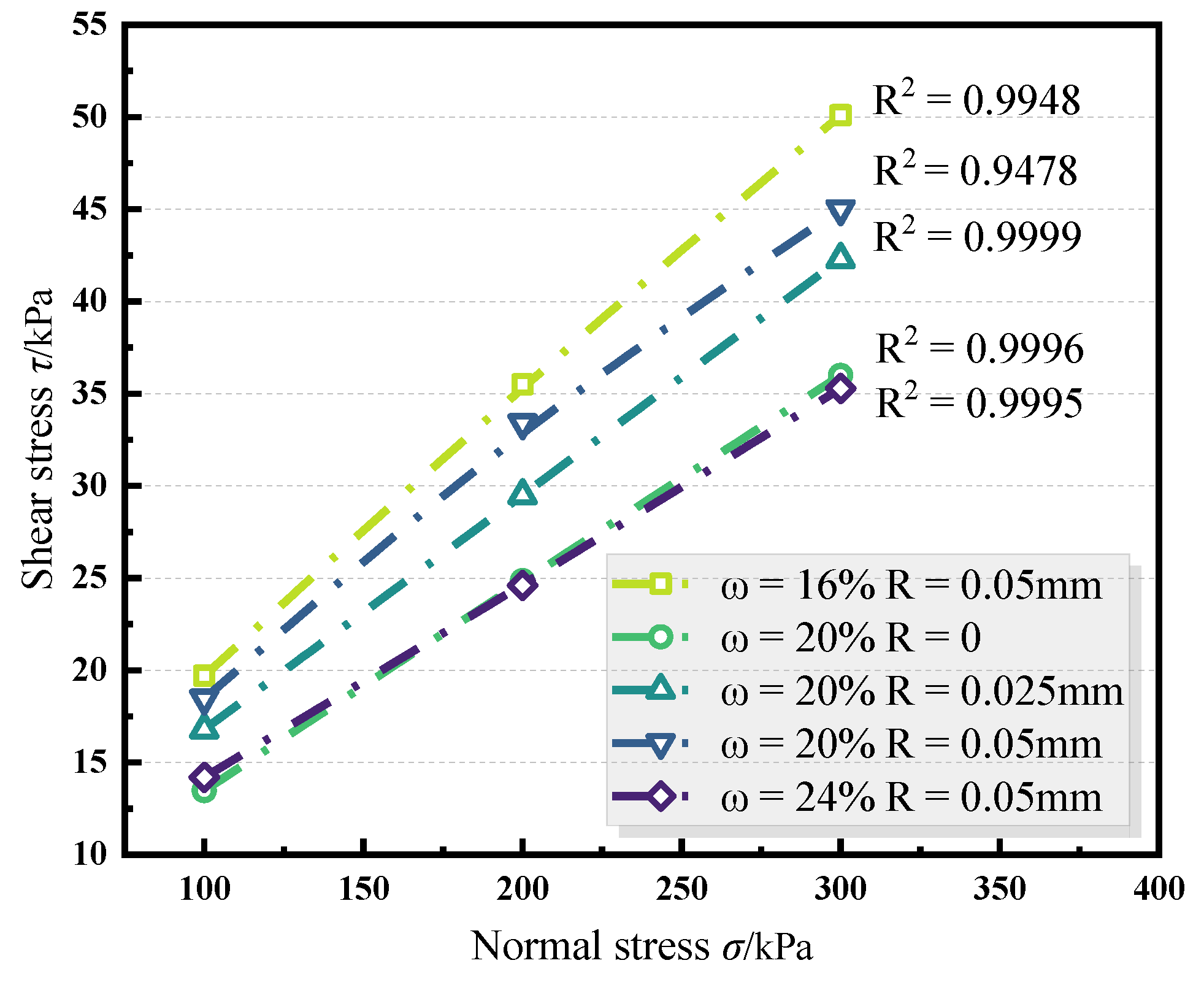
3.2.2. Interface Shear Strength

The relationship between peak shear stress/maximum shear stress and normal stress in this experiment was linearly fitted, as shown in Figure 5, with a good fit. The interface failure mode conforms to the Mohr–Coulomb failure criterion, namely:

$$\tau =\sigma \tan \phi +c$$

(16)

In the formula, σ is the vertical stress; φ is the apparent angle of internal friction; c is the apparent cohesive force.

(1)

Roughness

Figure 6a,b shows the shear strength and its parameters under different roughness conditions. The cohesion and internal friction angles corresponding to roughness R = 0, 0.025 and 0.05 mm are 2.25 kPa, 4.03 kPa, 5.76 kPa and 11.21°, 12.68° and 13.19°, respectively. As the roughness increases, the cohesion and internal friction angle increase 1.56 times and by 17.67%, respectively, indicating that the roughness greatly affects the interface cohesion. As the roughness increases, the depth of the structural groove deepens and the shear resistance required for soil particles to slip and roll increases; at the same time, the contact area between soil particles and the surface of the structure increases, leading to an increase in the filling of soil in the groove during the shear process, which enhances the bonding effect between the soil and the soil in the groove. At this point, the bonding strength becomes the main part of the shear strength. This pattern is more evident in the experiments of different groove structure steel plates with greater differences in roughness [31]. The friction angle refers to the friction between interfaces. As the roughness increases, the amount of soil filled into the groove increases, resulting in weakened friction between the soil and the smooth part of the structural surface (L₂), while the friction between the soil and the soil inside the groove increases, ultimately manifesting as a slight increase in the interface friction angle.

(2)

Water content

Figure 6c,d shows the shear strength and parameters under different water content conditions. The apparent cohesive force and apparent angle of internal friction corresponding to 16%, 20% and 24% water content are 4.7 kPa, 5.76 kPa, 3.61 kPa and 15.08°, 13.19° and 10.5°, respectively. As the water content increases, the cohesion shows a trend of first increasing and then decreasing, with increases of 22.6% and −59.5%, respectively, and the rate of growth at 16% to 20% is less than the rate of decrease at 20% to 24%. When the water content is low and then increases, the density of the soil sample increases, and at the same time, the adsorption effect of water between soil particles increases the soil cohesion. According to previous research, a peak of cohesion occurs when the water content reaches the plastic limit or the optimal water content [32]. In this study, the peak of cohesion appears near the optimal moisture content (19.6%); as the water content further increases, the thickness of the membrane water between soil particles increases, weak bonding water increases and free water begins to be generated. Soil particles separate under water pressure, and the contribution of structural suction to cohesion decreases, leading to a rapid decrease in cohesion. As the water content increases, the lubrication effect of the water film between the interfaces increases, and the internal friction angle shows a downward trend, with a decrease of 30.37%, indicating that the water content dramatically affects the internal friction angle of the contact surface.

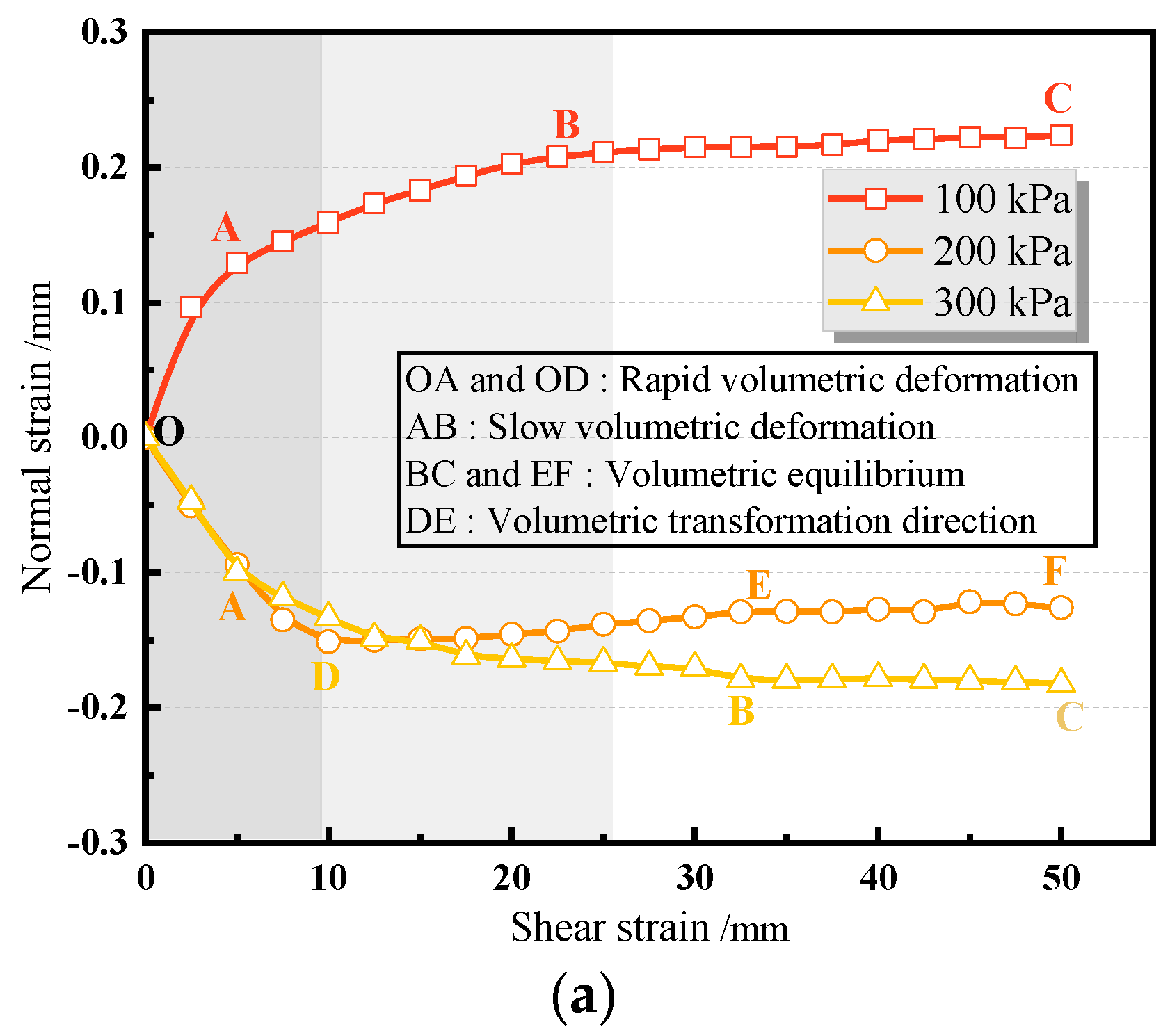
3.2.3. Volumetric Deformation Laws

The cross-sectional area of the shear interface in this experiment is a constant value. Therefore, its normal strain is measured to reflect the volume change of the sample during the shear process, which is the shear volumetric deformation laws of the interface.

(1)

Normal stress

Figure 7a shows the interface shear strain–normal strain curve under normal stress of 100 kPa, 200 kPa and 300 kPa, respectively (roughness R = 0.05 mm and water content ω = 20%).

It can be seen that while the roughness of the steel plate and the water content of the soil remain unchanged, the interfacial deformation patterns presented by different normal stresses are different. Under low-stress (σ = 100 kPa) conditions, the interface exhibits shear dilation. With the increase of normal stress, under medium stress (σ = 200 kPa) conditions, the interfacial deformation shows a pattern of initial shear shrinkage followed by slight shear dilation and overall reduction. The normal stress further increases, and under high-stress (σ = 300 kPa) conditions, the interface exhibits shear shrinkage. However, regardless of its shear shrinkage or shear expansion, the shear strain–normal strain curve can always be divided into three stages: rapid volumetric deformation stage (OA, OD), slow volumetric deformation stage (AB)/volumetric transformation direction stage (DE) and volumetric equilibrium stage (BC, EF). The soil bears a portion of the compaction work during the compaction process. During the shear process, due to the displacement of soil particles, the accumulated cohesive and frictional potential energy during the compaction process is released, resulting in an upward force. When the normal stress is low, this upward force and the normal stress offset the pressure difference, which is positive, thus exhibiting shear dilation; when the normal stress is high, the pressure difference between the upward force and the normal stress is negative, and the soil particle gap is compressed, thus exhibiting shear shrinkage [33].

In addition, the reason for the phenomenon of first shrinkage and then shear expansion under medium stress (σ = 200 kPa) may be that the previously compressed voids between soil particles undergo particle dislocation and restore some of the voids with the progress of shear, resulting in a phenomenon of the smaller volume first and then increasing volume.

(2)

Roughness

Figure 7b–d shows the shear strain–normal strain curves on three steel plates with different roughness, R = 0, 0.025 and 0.05 mm, under normal stress of 100, 200 and 300 kPa, respectively (water content ω = 20%). Under the same normal stress, the interface body becomes more significant as the roughness increases. To be more precise, in the low-stress shear expansion stage, the more significant the roughness, the greater the shear expansion amount; in the high-stress stage, the more significant the roughness, the greater the reduction. The increase in roughness enhances the degree of engagement between soil particles and the interface, leading to an increase in soil particles embedded in rough grooves and an increase in the thickness of the interface shear band [34], increasing volumetric deformation.

(3)

Water content

Figure 7e–g shows the shear strain–normal strain curves on three water contents soil samples at 16%, 20%, and 24% (with a water content of 15.9%, 19.8%, and 23.2% measured after the experiment) under normal stress of 100, 200, and 300 kPa, respectively (R = 0.05 mm). Under different normal stresses, lower water content (ω = 16%) consistently exhibits a certain degree of shear dilation. Even under high-stress conditions (σ = 300 kPa), shear strain–normal strain curves also exhibit a first shrinkage pattern and then shear dilation. The reason for this phenomenon may be due to the filling method. To control the dry density of the filled soil, soil samples with lower water content need to withstand more excellent compaction work so that the compacted soil may have over-consolidation properties [35]. At the same time, as the normal stress increases, the degree of bulk deformation changes less, indicating that under low water content conditions, the normal stress increases to a certain extent, and its impact on interface bulk deformation weakens. This is because the more significant the normal stress, the denser the soil compression and the weaker the water sensitivity, making the mechanical properties on the contact surface relatively less affected by the water content. However, high water content (ω = 24%) consistently exhibits shear shrinkage, even under low stress (σ = 100 kPa) conditions; the reason for this may be due to the high saturation of the soil sample (S_r = 95.2%) which causes a small amount of soil to be squeezed out during the test process, resulting in shear shrinkage. In addition, under the same normal stress, as the water content increases, the initial slope of the volumetric curve decreases, which has the same regularity as the shear stress–shear displacement curve mentioned above.

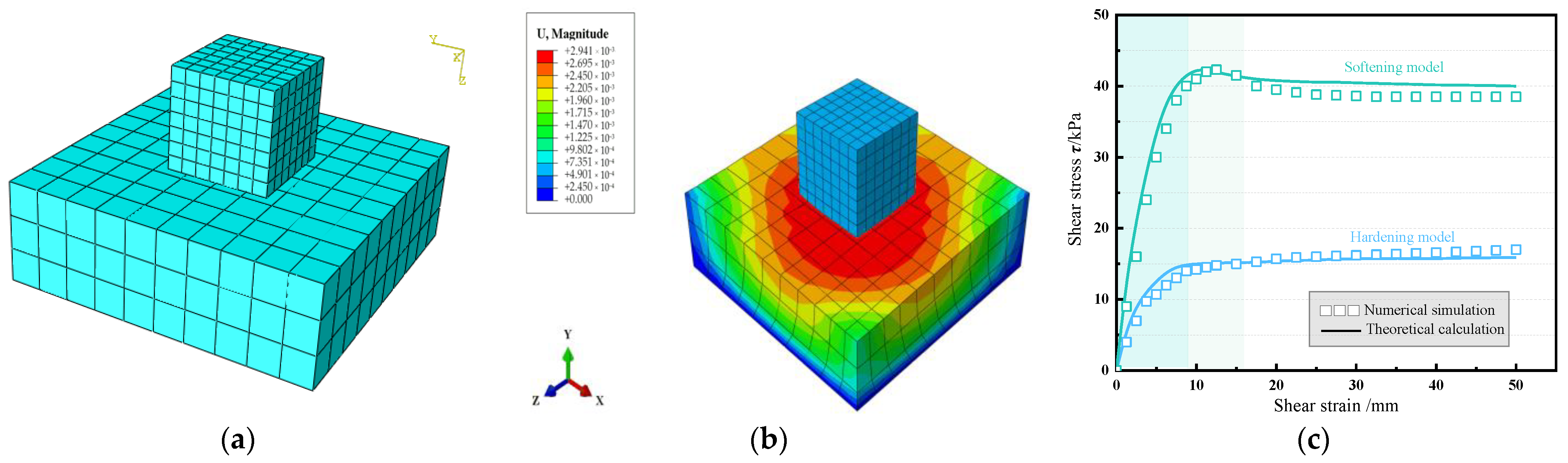
4. Model Validation and Numerical Implementation

4.1. Model Validation

According to the shear test results, the silt–steel interface exhibits a hardening curve under low to medium stress (σ = 100 kPa, 200 kPa) and medium to high water content (ω = 20%, 24%) conditions; it is a softening curve under high stress (σ = 300 kPa) and low to medium water content (ω = 16%, 20%) conditions.

For hardening curves, the strength parameter is τ_max, G₀ and G₁, with model parameters m and n; for softening curves, the strength parameters are τ_max, γ_m, τ_r and G₀, and the model parameters are m and n, respectively. The strength parameters were obtained through inverse calculation of the shear test results, where G₀ and G₁ were obtained from calculating initial shear modulus in material mechanics and Hooke’s law. G₀ under normal stress of 100 kPa, 200 kPa and 300 kPa was 23.13 MPa, 41.57 MPa and 74.89 MPa, respectively; the G₁ values under normal stress of 100 kPa and 200 kPa are 19.24 Mpa and 28.32 Mpa, respectively.

We selected the softening/hardening test data from the shear test and compared them with the model. Using the custom fitting function of MATLAB software, the m and n values under the above conditions can be obtained through regression analysis, as shown in

Table 2. Test group of hardening/softening type.

Test Conditions	τmax (kPa)		τr (kPa)		γm (mm)		m	n
	Test Value	Theoretical Value	Test Value	Theoretical Value	Test Value	Theoretical Value
Hardening type
σ = 100 kPa R = 0.05 mm ω = 20%	18.47	18.61					0.4271	4.4132 × 10−3
σ = 200 kPa R = 0.05 mm ω = 20%	33.43	33.53					0.3175	2.2541 × 10−3
σ = 100 kPa R = 0.025 mm ω = 20%	15.92	16.53					0.5137	4.6871 × 10−3
σ = 100 kPa R = 0.05 mm ω = 24%	14.21	13.71					0.5546	5.1247 × 10−3
Softening type
σ = 200 kPa R = 0.05 mm ω = 16%	35.53	35.01	33.28	33.01	12.4	13.6	0.2985	2.1187 × 10−3
σ = 300 kPa R = 0.05 mm ω = 16%	50.12	50.93	46.78	47.42	15.1	15.7	0.1782	1.7895 × 10−3
σ = 300 kPa R = 0.05 mm ω = 20%	45.08	46.61	41.14	42.33	12.6	14.3	0.2297	2.0891 × 10−3
σ = 300 kPa R = 0.025 mm ω = 20%	42.33	43.84	40.17	39.83	10.1	11.3	0.2457	2.1879 × 10−3

. The comparison curves of simulation and experimental results are plotted in Figure 8.

Table 2 shows that the theoretical calculation and shear test results under the four experimental conditions differ slightly for the hardening model. The theoretical values of the maximum shear stress τ_max differ by 0.7%, 0.3%, 3.8% and 3.5% compared to the experimental results. From Figure 8a, it can be seen that the theoretical calculation curve has a high degree of agreement with the shear test curve, which can accurately reflect the hardening characteristics. The hardening model in the damage model, based on the classical hyperbola model, can better simulate the stress–strain relationship of the silt–steel interface under conditions of low normal stress and high water content.

From Table 2, it can be seen that for the softening model, the theoretical calculation results and shear test results of the four experimental conditions also have slight differences, with the theoretical values of the maximum shear stress τ_max varying by 1.5%, 1.6%, 3.4% and 3.6%, respectively, compared to the test results; the theoretical values of residual shear stress τ_r differ by 0.8%, 2%, 2.9% and 0.8% compared to the experimental results, and the theoretical values of maximum shear stress displacement γ_m differ by 9.7%, 4%, 13.5% and 11.9% compared to the experimental results. From Figure 8b, it can be seen that there is a high degree of overlap between the theoretical calculation curve and the shear test curve. Although there is a slight separation between the curves in the initial shear and residual friction stages, they can show a softening trend. The softening model in the damage model, based on the classic rock damage model, can better simulate the stress–strain relationship at the high normal stress and low moisture content states of the silt–steel interface.

In summary, although the theoretical calculation results do not fully match the shear test results, considering factors such as calculation errors, model assumptions and soil complexity, the difference between the theoretical calculation curve and the shear test curve is within a reasonable range, indicating that the model can reflect the characteristics of softening strain at the silt–steel interface under high normal stress or low water content conditions and hardening strain under low normal stress or high water content conditions. The theoretical model is based on damage mechanics, the model parameters are easy to obtain and the accuracy is appropriate. The theoretical model is suitable for describing the shear failure process of the silt–steel structure interface in the Yellow River Delta.

It should be noted here that on the premise of determining the shear modulus G, since the model parameters m and n in the softening and hardening model are affected by normal stress, roughness and water content simultaneously, they cannot be modified by fitting curves. Considering the complexity of factors affecting the soil–structure interface in natural environments, the model still needs further optimization and improvement.

4.2. Numerical Implementation

The derivation and establishment of mathematical interface models aim to match numerical calculation methods and implement them in practical engineering applications. ABAQUS software is commonly used for simulating the stability of offshore structures [36].

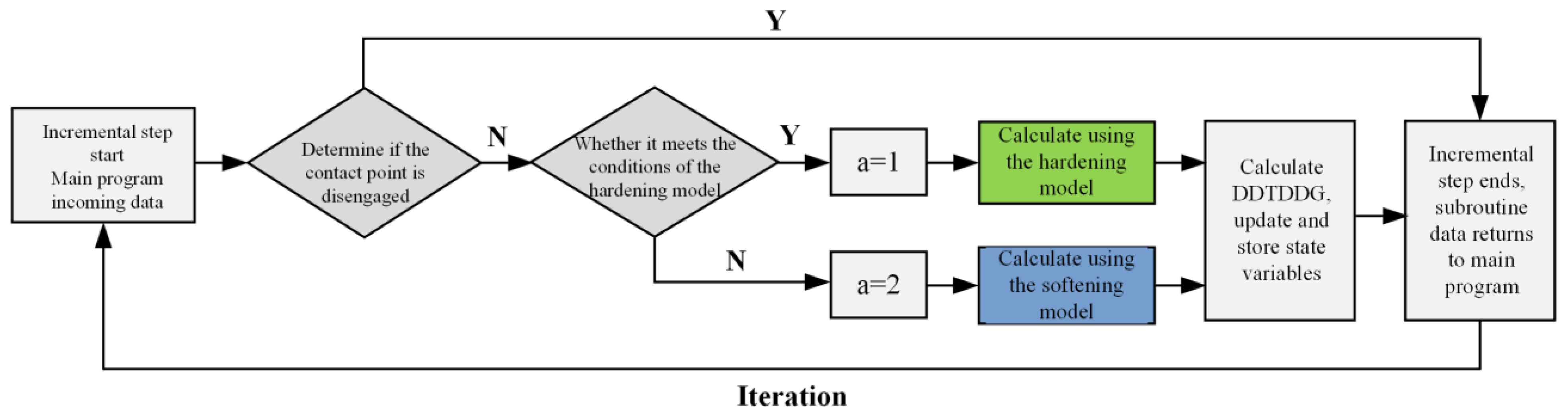
4.2.1. Subroutine Programming

To apply the damage model obtained in this paper to the future stability analysis of offshore wind power, FORTRAN language was used, referring to Yan (2020) [37] and Shi (2021) [38], and the subroutine design and code writing were carried out according to the FRIC subroutine format in ABAQUS. Considering the convergence of the calculation results and the saving of calculation time, the default thickness-free element is adopted, which does not consider the stiffness coefficient in the interface direction and only needs to provide the stiffness coefficient in the interface slip direction. Therefore, the interface has no thickness in the calculation, only length [39].

Because ABAQUS determines the slip and detachment of the contact surface, the FRIC subroutine only needs to define the friction characteristics on the interface, that is, select the constitutive relationship. The implementation process of the FRIC subroutine is shown in Figure 9. The subroutine is called once for each load increment step during the primary software calculation process. After the subroutine calculation, it returns to the main program to complete the iterative calculation of this loading step, ultimately achieving the implementation of the soft and hard damage model in ABAQUS.

4.2.2. Subroutine Validation

To verify the reliability of the FRIC subroutine, a simple slider finite element model is set up, as shown in Figure 10a, referring to the method proposed by Lu et al. (2017) [11] and Wang et al. (2012) [40]. The upper part is a 1 m × 1 m ×1 m soil block constructed using CAX4R elements. It should be noted that the Poisson’s ratio is set to v = 0 to ignore the influence of lateral deformation on shear. The lower part is a 3 m × 3 m ×1 m rigid block using CAX4I units; the main control surface is a rigid body surface with sparse mesh division, while the subordinate surface is a soil block surface with dense mesh division. The face-to-face discretization method is used to set the normal interaction relationship of its contact surface as the hard contact inherent in ABAQUS, and the tangential interaction is set using the developed FRIC subroutine.

According to the two cases of softening/hardening, the loading is divided into two analysis steps: ① apply normal stresses of 100 kPa (hardening type) and 300 kPa (softening type) to the surface of the soil and establish the contact between the two components; ② set up a soil test with a displacement of 0.05 m in the x-direction, that is, apply a load displacement of U = 0.05 m to simulate the shear process. The specific model parameters are shown in

Table 3. Model parameters.

Category	Elastic Modulus E (MPa)	Poisson’s Ratio v	Unit Weight γ (kN/m3)	Cohesion c (kPa)	Internal Friction Angle φ (°)
Rigid body	2.1 × 105	0.3	78	/	/
Soil mass	3	0	8	12	20
Category	G (MPa)	τr (kPa)	α (kPa)	m	n
Hardening	23.13	/	15.45	0.4271	4.4132 × 10−3
Softening	74.89	40.13	/	0.2297	2.0891 × 10−3

, and the dilation angle (ψ) of soil mass is 0.1°.

The comparison between the shear stress–strain curve simulated by the subroutine and the theoretical model results is shown in Figure 10b,c. It can be seen from the figure that the simulation results of the subprogram are highly consistent with the calculation results of the constitutive model, which can not only simulate the continuous increase of the strain hardening shear stress but also simulate the strain softening residual friction, which verifies the feasibility of the FRIC subprogram, indicating that the interface shear model established in this paper can be successfully realized in the finite element calculation software ABAQUS by using the subprogram FRIC. This provides a model foundation and technical support for future analysis of the bearing capacity of offshore structures considering interface weakening effects.

5. Conclusions

This article studies the pile–soil interaction of offshore structures. Taking steel and silt in the Yellow River Delta as test materials combined with a monotonic shear test under different normal stress, roughness and water content conditions, the shear mechanical properties of the silt–steel interface were studied. A soil–structure interface softening/hardening damage model based on Weibull distribution was proposed, and the damage model parameters were determined. Finally, the rationality of the model was verified.

(1)

Compared to the strain hardening, shear shrinkage deformation and strain softening, the shear expansion deformation behavior of coarse-grained soil and cohesive soil silt exhibits two characteristics: softening/hardening and shear shrinkage/expansion under different conditions. The maximum shear stress increases with normal stress, roughness, and water content increase. Roughness has a significant impact on cohesion. As roughness increases, the cohesion and internal friction angle increase 1.56 times and by 17.67%, respectively; water content mainly affects the internal friction angle. As the water content increases, the internal friction angle decreases, with a decrease of 30.37%. The cohesion shows a trend of increasing and then decreasing, with an increase of 22.6% and −59.5%, respectively, and reaches its peak near optimal water content.

(2)

The proposed shear damage model has fewer parameters and a clear physical meaning. The strength parameters are τ_max, G₀, G₁, γ_m, τ_r, and the model parameters are m and n. The softening model, based on the classic rock damage model, can better simulate the stress–strain relationship of the silt–steel interface under high normal stress and low water content. In contrast, the hardening model based on the classic hyperbola model can better simulate the stress–strain relationship under low normal stress and high water content. After using the model parameters obtained from the test results, the theoretical model curve is in good agreement with the shear test curve, which proves that the proposed contact surface damage model is reasonable. However, the model parameters m and n are simultaneously affected by normal stress, roughness and water content, so they cannot be simply corrected by fitting curves. Considering the complexity of factors affecting the soil–structure interface in real environments, the model still needs further optimization and improvement.

(3)

The numerical simulation application of the damage model was achieved through the FRIC subroutine, providing a mathematical model basis for subsequent research on the stability analysis of offshore structures considering interface weakening effects.

References

1. Guo, X.; Fan, N.; Liu, Y.; Liu, X.; Wang, Z.; Xie, X.; Jia, Y. Deep seabed mining: Frontiers in engineering geology and environment. Int. J. Coal Sci. Technol. 2023, 10, 23. [Google Scholar] [CrossRef]
2. Yu, P.; Liu, H.; Wang, Z.; Fu, J.; Zhang, H.; Wang, J.; Yang, Q. Development of urban underground space in coastal cities in China: A review. Deep. Undergr. Sci. Eng. 2023, 2, 148–172. [Google Scholar] [CrossRef]
3. Yu, P.; Hu, R.; Yang, J.; Liu, H. Numerical investigation of local scour around USAF with different hydraulic conditions under currents and waves. Ocean Eng. 2020, 213, 107696. [Google Scholar] [CrossRef]
4. Zhang, Y.; Feng, X.; Ding, C.; Liu, Y.; Liu, T. Study of cone penetration rate effects in the Yellow River Delta silty soils with different clay contents and state parameters. Ocean Eng. 2022, 250, 110982. [Google Scholar] [CrossRef]
5. Ravera, E.; Laloui, L. Failure mechanism of fine-grained soil-structure interface for energy piles. Soils Found. 2022, 62, 101152. [Google Scholar] [CrossRef]
6. Hashemi, A.; Sutman, M.; Medero, G.M. A review on the thermo-hydro-mechanical response of soil–structure interface for energy geostructures applications. Géoméch. Energy Environ. 2023, 33, 100439. [Google Scholar] [CrossRef]
7. Liu, J.; Zou, D.; Kong, X. A three-dimensional state-dependent model of soil–structure interface for monotonic and cyclic loadings. Comput. Geotech. 2014, 61, 166–177. [Google Scholar] [CrossRef]
8. Stutz, H.; Mašín, D.; Wuttke, F. Enhancement of a hypoplastic model for granular soil–structure interface behaviour. Acta Geotech. 2016, 11, 1249–1261. [Google Scholar] [CrossRef]
9. Hosseinali, M.; Toufigh, V. A plasticity-based constitutive model for the behavior of soil-structure interfaces under cyclic loading. Transp. Geotech. 2018, 14, 41–51. [Google Scholar] [CrossRef]
10. Saberi, M.; Annan, C.-D.; Konrad, J.-M. Three-dimensional constitutive model for cyclic behavior of soil-structure interfaces. Soil Dyn. Earthq. Eng. 2020, 134, 106162. [Google Scholar] [CrossRef]
11. De-chun, L.U.; Lei, L.; Xin, W.; Xiu-li, D.U. Softening/Hardening constitutive model for soil-structure interface and numerical implementation. Eng. Mech. 2017, 34, 41–50. [Google Scholar] [CrossRef]
12. Ajcinovic, K.R.D.; Silva, M.A.G. Statistical of the continuous damage theory. Int. J. Solids. Struct. 1982, 19, 551–562. [Google Scholar] [CrossRef]
13. Hu, L.; Pu, J. Testing and Modeling of Soil-Structure Interface. J. Geotech. Geoenviron. 2004, 130, 851–860. [Google Scholar] [CrossRef]
14. Long, Y.; Chen, J.; Zhang, J. Introduction and analysis of a strain-softening damage model for soil–structure interfaces considering shear thickness. KSCE J. Civ. Eng. 2017, 21, 2634–2640. [Google Scholar] [CrossRef]
15. Zhao, L.; Yang, P.; Zhang, L.-C.; Wang, J. Cyclic direct shear behaviors of an artificial frozen soil-structure interface under constant normal stress and sub-zero temperature. Cold Reg. Sci. Technol. 2017, 133, 70–81. [Google Scholar] [CrossRef]
16. Zhu, Z.W.; Guo, Z. Temperature damage and constitutive model of frozen soil under dynamic loading. Mech. Mater. 2016, 102, 108–116. [Google Scholar] [CrossRef]
17. Chen, W.; Luo, Q.; Liu, J.; Wang, T.; Wang, L. Modeling of frozen soil-structure interface shear behavior by supervised deep learning. Cold Reg. Sci. Technol. 2022, 200, 10358. [Google Scholar] [CrossRef]
18. Sun, K.; Tang, L.; Zhou, A.; Ling, X. An elastoplastic damage constitutive model for frozen soil based on the super/subloading yield surfaces. Comput. Geotech. 2020, 128, 103842. [Google Scholar] [CrossRef]
19. Liu, L.; Ji, H.; Elsworth, D.; Zhi, S.; Lv, X.; Wang, T. Dual-damage constitutive model to define thermal damage in rock. Int. J. Rock Mech. Min. Sci. 2019, 126, 104185. [Google Scholar] [CrossRef]
20. Rehman, Z.; Zhang, G. Three-dimensional elasto-plastic damage model for gravelly soil-structure interface considering the shear coupling effect. Compu. Geotech. 2021, 129, 103868. [Google Scholar] [CrossRef]
21. Yang, Q.; Zheng, Z.; El Naggar, M.H.; Kong, G.; Zhang, S.; Yang, G.; Ren, Y. Experimental study of the interface evolution behavior and softening mechanism of structure-marine soil. Soils Found. 2023, 63, 101324. [Google Scholar] [CrossRef]
22. Zhang, P.; Fei, K.; Dai, D. Modeling of granular soil-structure interface under monotonic and cyclic loading with the nonlinear approach. Comput. Geotech. 2023, 159, 105480. [Google Scholar] [CrossRef]
23. Clough, G.W.; Duncan, J.M. Finite element analysis of retaining wall behavior. J. Soil. Mech. Found 1971, 97, 1657–1672. [Google Scholar] [CrossRef]
24. Yu, P.; Dong, J.; Liu, H.; Xu, R.; Wang, R.; Xu, M.; Liu, H. Analysis of Cyclic Shear Stress–Displacement Mechanical Properties of Silt–Steel Interface in the Yellow River Delta. J. Mar. Sci. Eng. 2022, 10, 1704. [Google Scholar] [CrossRef]
25. Lemaiter, J. A continuous damage mechanics model for ductile materials. J. Eng. Mater. Techno. 1985, 107, 83–89. [Google Scholar]
26. Yu, P.; Dong, J.; Guan, Y.; Wang, Q.; Jia, S.; Xu, M.; Liu, H.; Yang, Q. Experimental Investigation on the Cyclic Shear Mechanical Characteristics and Dynamic Response of a Steel–Silt Interface in the Yellow River Delta. J. Mar. Sci. Eng. 2023, 11, 223. [Google Scholar] [CrossRef]
27. Su, L.-J.; Zhou, W.-H.; Chen, W.-B.; Jie, X. Effects of relative roughness and mean particle size on the shear strength of sand-steel interface. Measurement 2018, 122, 339–346. [Google Scholar] [CrossRef]
28. Abdulrahman, A.A.; Rayhani, M. Interface shear strength characteristics of steel piles in frozen clay under varying exposure temperature. Soils. Found. 2019, 59, 2110–2124. [Google Scholar] [CrossRef]
29. Ma, X.; Lei, H.; Kang, X. Examination of interface roughness and particle morphology on granular soil–structure shearing behavior using DEM and 3D printing. Eng. Struct. 2023, 290, 116365. [Google Scholar] [CrossRef]
30. Chusak, K. Effect of oil-contamination and water saturation on the bearing capacity and shear strength parameters of silty sandy soil. Eng. Geol. 2019, 257, 105138. [Google Scholar] [CrossRef]
31. Wang, T.-L.; Wang, H.-H.; Hu, T.-F.; Song, H.-F. Experimental study on the mechanical properties of soil-structure interface under frozen conditions using an improved roughness algorithm. Cold Reg. Sci. Technol. 2019, 158, 62–68. [Google Scholar] [CrossRef]
32. El Hariri, A.; Ahmed, A.E.E.; Kiss, P. Review on soil shear strength with loam sand soil results using direct shear test. J. Terramech. 2023, 107, 47–59. [Google Scholar] [CrossRef]
33. Jiang, Q.; Yang, Y.; Yan, F.; Zhou, J.; Li, S.; Yang, B.; Zheng, H. Deformation and failure behaviours of rock-concrete interfaces with natural morphology under shear testing. Constr. Build. Mater. 2021, 293, 123468. [Google Scholar] [CrossRef]
34. Timbolmas, C.; Bravo, R.; Rescalvo, F.J.; Villanueva, P.; Portela, M. Digital image correlation and numerical analysis of CFRP-poplar timber interface subjected to modified single shear test. Compos. Struct. 2023, 320, 117188. [Google Scholar] [CrossRef]
35. Yang, W.; He, J.; Liu, L.; Yang, H. Testing the shearing creep of composite geomembranes-cushion interface and its empirical model. Soils Found. 2022, 62, 101236. [Google Scholar] [CrossRef]
36. Guo, X.; Nian, T.; Fu, C.; Zheng, D. Numerical Investigation of the Landslide Cover Thickness Effect on the Drag Forces Acting on Submarine Pipelines. J. Waterw. Port Coast. Ocean Eng. 2023, 149, 04022032. [Google Scholar] [CrossRef]
37. Yan, D.J. Numerical Simulation Analysis of Interfacial Mechanical Behavior of Concrete Structures Strengthened by CFRP Grid-Polymer Cement Mortar (PCM). Master’s Thesis, Chang an University, Xi’an, China, 2020. (In Chinese). [Google Scholar]
38. Shi, F. Numerical Simulation of Interfacial Debonding between FRP and Concrete under Fatigue Loading. Master’s Thesis, China University of Petroleum, Beijing, China, 2021. (In Chinese). [Google Scholar]
39. Wang, F.L. Experimental Study and Finite Element Simulation of Interfacial Bond Behavior of CFRP- Concrete under Cyclic Loading. Master’s Thesis, Qingdao University of Technology, Qingdao, China, 2021. (In Chinese). [Google Scholar]
40. Wang, W.D.; Li, Y.H.; Wu, J.B. Pile-soil interface shear model of super long bored pile and its FEM simulation. Rock Soil Mech. 2012, 33, 3818–3824+3832. (In Chinese) [Google Scholar] [CrossRef]
Figure 1. Offshore wind power. (a) China’s first far-reaching offshore floating wind power platform, the “Sea Oil Mission”. (b) The first demonstration project for the integration of marine ranching and affordable offshore wind power in Shandong Province. (c) OWT planning map of Shandong.
Jmse 11 01415 g001
Figure 2. Soil–structure interface damage hypothesis.
Jmse 11 01415 g002
Figure 3. Test equipment. (a) Schematic diagram of steel plates with different roughness. (b) Roughness parameter. (c) Large-scale interface shear instrument [24,26].
Jmse 11 01415 g003
Figure 4. Shear stress–strain curves under different normal stress (100 kPa, 200 kPa, 300 kPa). (a) The influence of normal stress. (bd) The influence of roughness. (eg) The influence of water.
Jmse 11 01415 g004
Figure 5. Fitting curves of the shear strength.
Jmse 11 01415 g005
Figure 6. Shear strength and parameters. (a,b) Under different roughness. (c,d) Under water content.
Jmse 11 01415 g006
Figure 7. Shear stress–normal strain curves under different normal stress (100 kPa, 200 kPa, 300 kP). (a) The influence of normal stress. (bd) The influence of roughness. (eg) The influence of water content.
Jmse 11 01415 g007aJmse 11 01415 g007b
Figure 8. Comparison between theoretical and experimental results. (a) Hardening model. (b) Softening model.
Jmse 11 01415 g008
Figure 9. Implementation process of subroutine.
Jmse 11 01415 g009
Figure 10. Subroutine validation. (a) Slider simulation. (b) Strain output results (c) Comparison of results.
Jmse 11 01415 g010