Abstract
The paper analyzes quasiperiodic upwellings and downwellings on the shelf and upper part of continental slope of the northeastern Black Sea. It is shown that these processes are related to changes in intensity and direction of alongshore current and the following geostrophic adjustment of the density field. The source of such changes is the meandering of the Black Sea Rim Current (RC). It leads to a quasiperiodic change in direction of the alongshore current, from northwestern (cyclonic RC meander) to southeastern (anticyclonic RC meander, or eddy). These cycles, or phases, have an average duration of about 10 days. During the northwestern phase, the permanent Black Sea pycnohalocline (hereafter pycnocline) and seasonal thermocline descend, their thickness increases, and so does the thickness of the upper mixed layer (UML). During the southeastern phase, both the pycnocline and seasonal thermocline ascend and become thinner, along with the UML, which also becomes thinner. In both phases, isopycnals in the pycnocline and isotherms in the thermocline demonstrate quasi-in-phase vertical oscillations, which have a good correlation with the speed and direction of the alongshore current. These correlations allow estimation of the magnitude of upwellings and downwellings in the shelf–slope area of the northeastern Black Sea using data series of current velocity profiles.
Keywords:
upwelling; downwelling; Black Sea; Rim Current; permanent pycnocline; seasonal thermocline 1. Introduction
The physical nature of upwellings in the World Ocean is usually attributed to wind impact, Ekman transport of surface water away from the shore, and the compensating upward movement of deep water [1,2,3,4]. In the coastal zone of the Black Sea, wind is also considered a major reason beyond the upwelling events [5]. At the same time, the direction and intensity of alongshore geostrophic currents in the upper ocean layer play an important role in upwelling and downwelling formation, and such currents often have no direct connection to the wind [6,7].
It is well known that most intense upwellings are observed in the Eastern Boundary Currents, such as Canary, Benguela, California, Peru, etc. [8]. The geostrophic dynamics of these currents push isopycnal and isothermal surfaces upward while wind force generates the offshore Ekman transport that amplifies the water rise. The combined effect of these two factors produces a permanent upwelling, which significantly increases the biological productivity of the euphotic layer [9,10]. In turn, the dynamics of the Western Boundary Currents, such as the Gulf Stream, Kuroshio, Brazil, East Australian, etc., push isopycnal and isothermal surfaces downwards and generate downwelling, which improve the oxygenation of deeper layers but hamper biological production in the surface layer.
The Black Sea is characterized with a cyclonic circulation, which affects the entire basin and causes water to rise in the central part and descend at the periphery. The main structural element of this circulation is the Rim Current [11,12,13], a downwelling and baroclinic current with maximum velocity near the surface. The RC velocity rapidly decreases with depth, slowing almost to a halt at 250–300 m [14] due to a sharp pycnocline. The pycnocline is located at 50–200 m depth, and vertical turbulent transfer is heavily suppressed in this layer. The RC core is generally situated near the base of the Black Sea continental slope, about 10–30 km from the shore in the northeastern part (where the shelf and continental slope are narrow), and 50 km and further from the shore in the northwestern part (where the shelf and continental slope are wide) [15,16,17]. The velocity inside the RC core occasionally reaches 1 m/s or greater, but the average speed of the RC is 0.15–0.20 m/s [18].
The RC and the central sea upwelling are mostly caused by a large-scale wind force, which has a cyclonic vorticity in the Black Sea region [19,20,21]. This vorticity increases during late autumn and winter, and decreases in spring and summer. Correspondingly, both the RC and central sea upwelling become stronger during the cold season and weaker in the warm season. The RC dynamics, especially during its weaker periods, include baroclinic instability, jet meandering, and generation of mesoscale eddies (mostly anticyclonic) [21,22,23,24]. Due to the meandering, in the northeastern part of the sea, where the shelf–slope zone is narrow, the RC core sometimes gets close to the shore (cyclonic meander) and sometimes moves away (anticyclonic meander, or eddy) [25]. As a result, the current in the coastal zone exhibits mostly a bimodal behavior [22,26]. A cyclonic meander causes intensification of the northwestern current [27]. An anticyclonic meander produces an anticyclonic eddy and changes the alongshore current direction to southeast.
Recent studies based on modeling [28] showed that RC interaction with topographic irregularities could also provide a certain input into the formation of mesoscale eddies in the northeastern Black Sea. The shoal near Pitsunda may act as a trigger for the formation of mesoscale eddies, which slowly travel northwest towards Gelendzhik and Novorossiysk.
Regular long-term studies on the upper part of the continental slope, performed with the Aqualog profiler [29] at the moored station near Gelendzhik, have shown that the average duration of one current oscillation cycle (when the alongshore current flows northwest and then southeast) is about 10 days (range 5–15 days). This variability has a synoptic time scale (i.e., from a few days to two weeks).
Since the Aqualog also collects salinity and temperature profiles (CTD data) along with current velocity profiles, it was found that the vertical position of isopycnals in the pycnocline and isotherms in the thermocline depend on the alongshore current direction. The isolines ascend during the southeastern current and descend when it turns northwest. The range of their vertical synoptic time scale oscillations can reach 70–80 m [30], which is comparable with the seasonal dynamics of their vertical position.
Thus, while the coastal geostrophic current in the northeastern Black Sea is mostly of the downwelling type, during some periods it changes direction, producing an upwelling. In most cases, such an upwelling is incomplete, i.e., it does not bring thermocline water to the surface. Nevertheless, the isotherms during this event rise upwards significantly, and if their rise is further amplified with a northwestern or northern wind, a complete upwelling may occur. It was found that while “non-wind” incomplete upwellings and downwellings occur quite often, they rarely coincide with correspondingly upwelling or downwelling wind forcing [31].
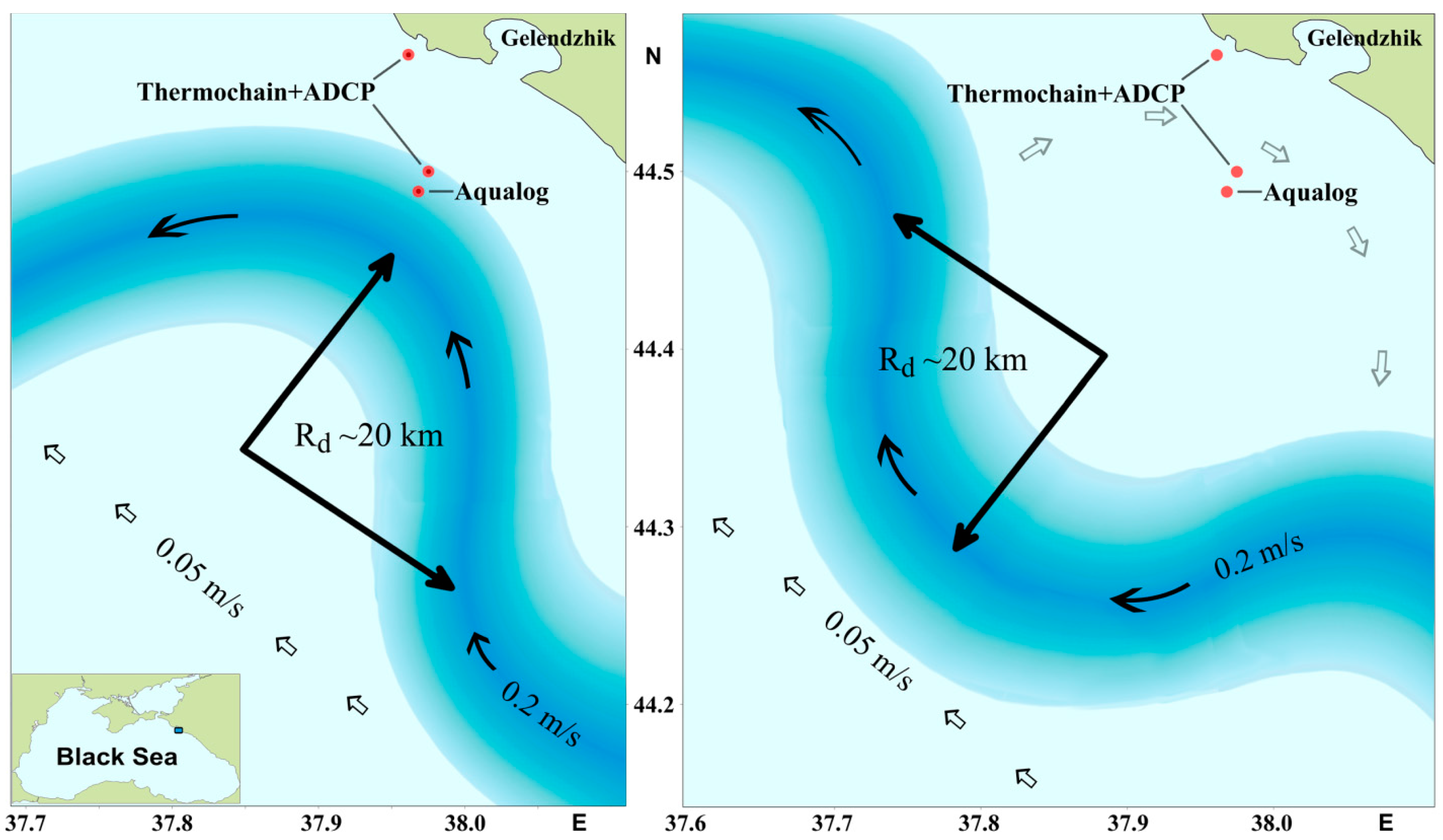
The described upwelling and downwelling oscillations correspond closely to a mathematical model of geostrophic adjustment. For simplicity, let us take a two-layer stratified fluid, with a thin upper layer (200 m), as compared with the lower layer (2000 m). We also assume that a cyclonic basin-scale rim current is present in the upper layer and absent in the lower layer (a purely baroclinic case). In this case, the spatial variation of sea level, which is a driving force of the current in the upper layer, is fully compensated in the lower level due to the curvature of the density boundary between the layers. The current core, generally distanced from the shelf by the baroclinic deformation radius Rd, approaches the shelf edge during a cyclonic meander and moves off the edge during an anticyclonic meander (Figure 1). In the context of the two-layer model,
Rd = (g′H)1/2/f

Figure 1.
Meandering of the Rim Current and periodic change in direction of the alongshore current in the studied area. On the left—a cyclonic meander, where the RC jet gets close to the coast. On the right—an anticyclonic meander, where the RC jet moves off the coast and a reverse flow (shown as wide arrows) forms near the shore. The red dots indicate positions of measuring stations (Aqualog, thermochains, and ADCPs).
Here, g′ = g∆ρ/ρ is the reduced acceleration of gravity, ∆ρ/ρ is the relative difference of density between the layers, H is the average height of the upper layer (including pycnocline), and f is the Coriolis parameter. Using typical values for the Black Sea, ∆ρ/ρ = (1.5–2.0)·10−3, H = 150–200 m, f = 10−4 s−1, and the resulting Rd = (15–25)·103 m = 15–25 km. This estimation is almost identical to the value acquired in [18] with a more sophisticated method and very close to the results of other approaches [11,32]. Suppose that the meander radius is about the same as Rd; the current velocity in the middle of the meander is zero, while on its edge, in the current core, the velocity is maximal. Due to geostrophic adjustment, the depth of the boundary between the two layers will be different on the edge of the meander and in the middle of the meander. This depth difference will be denoted as ∆H. Then, the current velocity on the edge of the meander, ∆U, estimated with the geostrophic approximation, can be defined as
∆U = g′∆H/(Rdf)
Let us assume a cyclonic direction for ∆U (i.e., northwest in a cyclonic meander) as positive. Then, from (2), it follows that ∆H is also positive and the boundary between the layers deepens towards the shore. In the opposite case, we have a southeastern coastal current in an anticyclonic meander, ∆H is negative, and the boundary rises up towards the shore. From (2), it follows that
and for ∆U = 0.30 m/s, g′ = 2·10−2 m/s2, and Rd = 2·104 m, ∆H = 30 m. Since the velocity difference can be even larger, the absolute value of ∆H can exceed the above estimation and the peak-to-peak amplitude S = 2∆H between cyclonic and anticyclonic meanders can reach 70–80 m. Such values are indeed observed in reality from time to time.
∆H = (Rdf∆U)/g′,
Let us assess the applicability of the geostrophic approximation to RC meanders and eddies with the radius of Rd and maximal orbital velocity ∆U = 0.30 m/s by calculating the respective Rossby number, Ro:
Ro = ∆U/(Rdf) = 0.15
This value is significantly lower than unity; therefore, the dynamics of the RC-generated meanders and eddies, as a first approximation, can be assumed to be geostrophic.
On the basis of satellite altimetry, it was shown [33] that the typical velocity of eddies and RC meanders along the coast in the northeastern Black Sea is about 0.05 m/s and directed northwest. For simplicity, let us assume that RC meanders are “frozen” and retain their shape while moving along the coast. Therefore, for a cyclonic meander to be replaced with an anticyclonic one, their alongshore drift should amount to 2Rd = 4·104 m = 40 km, which would take the time t = 4·104/0.05 = 8·105 s ≈ 9.3 days (Figure 1).
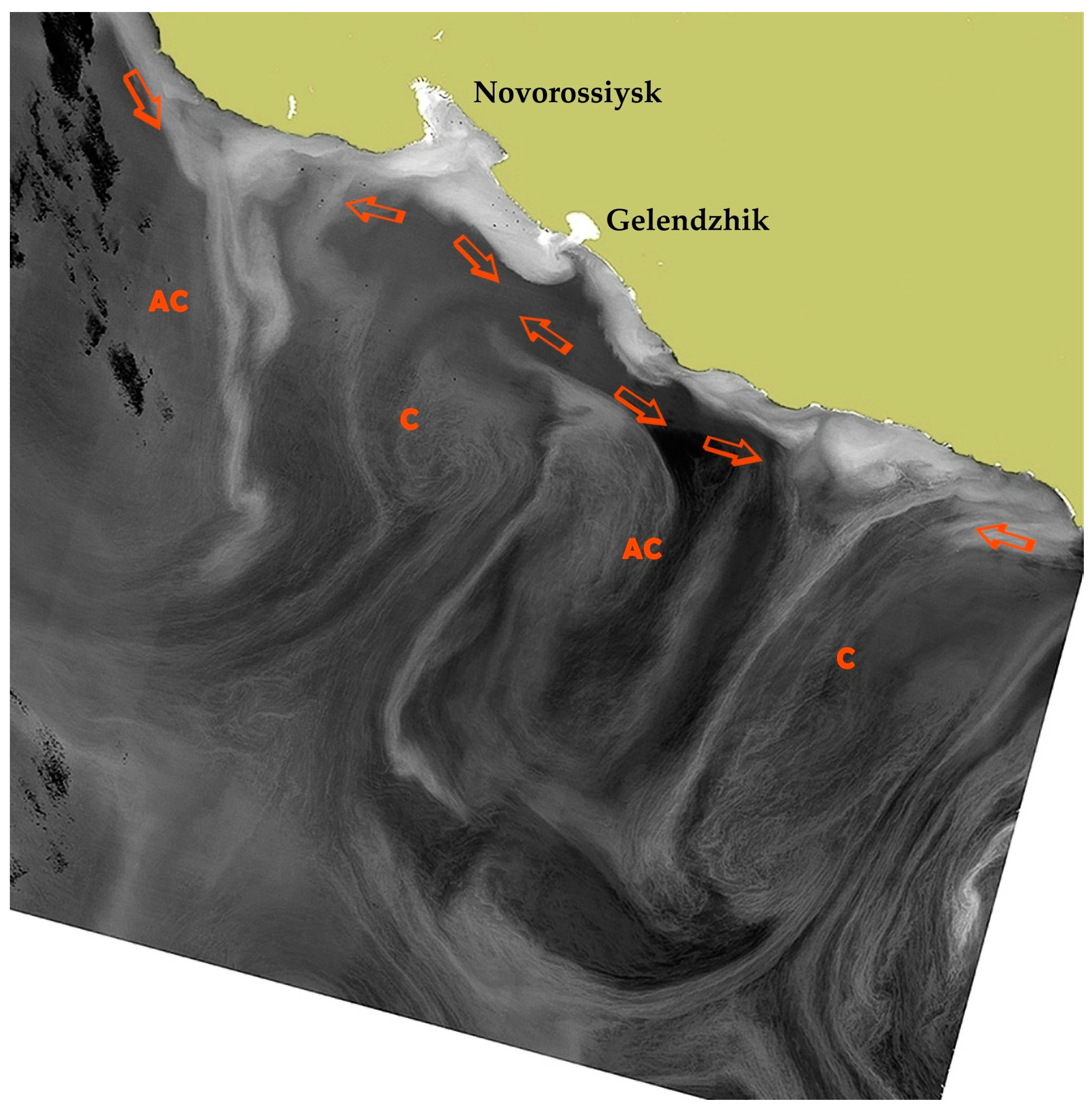
Although the above description of the RC dynamics, its meanders, and eddies is very simplified, occasionally it is confirmed by satellite data. Figure 2 shows a satellite image of the northeastern Black Sea, with a chain of cyclonic and anticyclonic eddies that generate oppositely directed alongshore currents.

Figure 2.
Satellite image of the northeastern Black Sea (Landsat 8, Operational Land Imager), 28 April 2015. AC—anticyclonic mesoscale eddies, C—cyclonic mesoscale eddies. Red arrows show alongshore current direction. Size of the eddies can be roughly estimated based on the distance between Novorossiysk and Gelendzhik (about 30 km in a straight line).
Therefore, the observed rise and descend of isopycnals and isotherms inside the Black Sea pycnocline, with a typical period of 10 days, can be considered geostrophic, caused by cyclonic and anticyclonic RC meanders that follow each other and move northwest along the coast. Based on the long-term (5.5 years), near-continuous measurements at moored buoy stations [14], it was found that the average number of direction-changing cycles for the alongshore current is 32 per year (range 19–46), corresponding to the average period of 11 days, which is very close to our estimation.
So far, however, there have been no quantitative studies of connection between vertical position of isopycnals and current velocity dynamics on a synoptic time scale in the Black Sea. It is unknown whether these changes are in-phase or if there is a time lag. It is unclear how oscillations of the alongshore current velocity are reflected in the thermocline, both on the continental slope and shelf, and how large the difference is between the thermocline and pycnocline oscillations, and their periods and amplitudes.
This paper tries to answer these questions using the long-term measurements of moored Aqualog profilers, bottom acoustic Doppler current profilers (ADCP), and thermistor chains, installed near the ADCPs. These high-frequency detailed data provide the means to study the dynamics of current velocity and isopycnals inside the pycnocline, as well as variations of current velocity and isotherms inside the seasonal thermocline.
The description of data and methods is provided in the next section. The results are given after that, followed by the discussion, and the summary of main results concludes the paper.
2. Materials and Methods
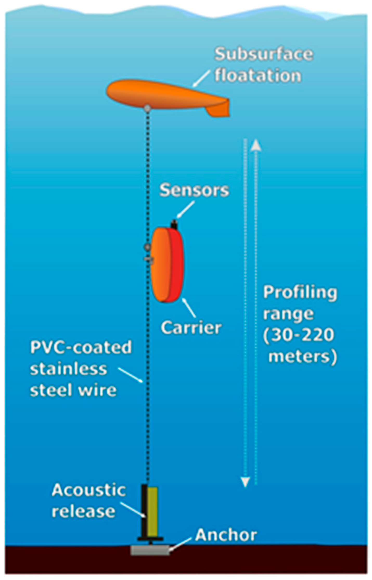
The analyzed data were acquired in the northeastern part of the Black Sea, near Gelendzhik. The autonomous moored profiler Aqualog (Figure 3) was set up on the continental slope, at about 250 m depth and 5 nautical miles from the shore. The profiler operated continuously from January 2016 to February 2017, with a few necessary maintenance breaks, collecting more than 1100 CTD and current velocity profiles over 286 days. The Aqualog is capable of moving up and down along a mooring line stretched between a bottom anchor and a subsurface floatation. The latter was positioned about 30 m below the sea surface—deep enough to avoid any significant effect on it from surface waves.
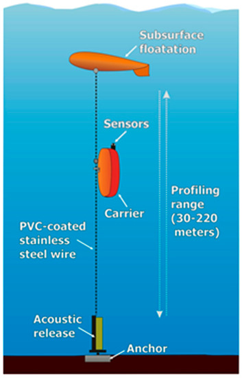
Figure 3.
The layout of the Aqualog profiler mooring station.
Due to the stable propulsive force and the streamline body of the device, its speed along the mooring cable was stable (about 20 cm/s in average, varying within a few cm/s). The Aqualog was equipped with the CTD probe Idronaut Ocean Seven 316 to measure temperature and salinity with a vertical resolution of 8–10 cm and the Doppler acoustic current meter Nortek Aquadopp 3D to measure current velocity with a vertical resolution of about one meter.
Bottom ADCP and a moored thermistor chain were installed in the same time and in the same area of continental slope as the Aqualog, only 2 km closer to the shore, at a depth of 86 m. This pair of devices will be further referred to as “deep ADCP and thermochain”, to differ them from another ADCP and thermochain pair, installed on the inner shelf (see below). Temperature was measured in a layer of 10–70 m, with an accuracy of ±0.01 °C. The ADCP (Teledyne RDI WHN Workhorse Sentinel, 300 kHz) was mounted inside a protective pyramid and set on the sea floor at a distance 100–150 m from the thermochain. The deep ADCP and thermochain were functioning from the end of March to November 2016, with a 19-day maintenance break (214 working days in total).
The third source of data was another ADCP and thermochain pair, working together at 26 m depth and 1.3 km from the shore. This pair of devices, called “nearshore ADCP and thermochain”, was connected online to a computer in a coastal laboratory via an armored underwater fiber-optic cable. These measurements were performed from the beginning of April to mid-July 2017, with a 7-day maintenance break (98 working days in total).
The locations of all three sets of the devices are shown in Figure 1. Frequency and resolution of the profilers were as follows. The Aqualog measured the detailed vertical profile from bottom to the subsurface floatation 4 times a day. Deep ADCP and thermochain measured profiles of temperature and current velocity every 4 min. Nearshore ADCP and thermochain measured profiles of temperature and current velocity every 30 s. The Aqualog data were binned into 1 m vertical cells. Distance between thermistors on the deep thermochain was 2 m; on the nearshore thermochain, the distance was 1 m. Vertical resolutions of the ADCPs were set to match the nearby thermochain.
As a preliminary processing step, the thermochain and ADCP data were smoothed with a moving average in a 1 h window. After that, to remove short-period, near-inertial oscillations (16–18 h), all data, including the Aqualog, were smoothed in a 2-day window. In the case of Aqualog, temporal smoothing was performed along isopycnals rather than depth coordinates, since distribution of main hydrophysical parameters (temperature, flow velocity, etc.) in the Black Sea depends on density and the gradient of these parameters along density surfaces is very small. Because of that, temporal averaging for the Black Sea pycnocline results as more accurate (with a far lower number of fluctuations) when performed on density coordinates. For that purpose, the primary data, initially binned into 1 m vertical cells, were re-binned into isopycnal layers with a uniform vertical step of 0.01 kg/m3. An Akima spline [34] was used to interpolate the data over the thicker density grid. After this transformation, a 2-day moving average was applied to each individual isopycnal within the potential density range from 14.1 to 16.3 kg/m3. The density limits were chosen to ensure that the selected density range was almost always within the depth limits of the studied layer. While the top and bottom depths of the Aqualog profiles remained mostly the same, water density varied significantly and a wider density interval would result in more data gaps near the endpoints of the profiles.
Neither the ADCPs nor the thermochains measured density; thus, temporal smoothing in their case was performed on depth coordinates. However, since the water layer, measured by these devices, was situated above the pycnocline and mostly included the seasonal thermocline and the upper mixed layer (UML), where salinity input into density is minor, the lack of density connection in this case does not appear to be of large significance.
The studied area is dominated by alongshore currents, and the alongshore velocity component is usually 5–10 times higher than the cross-current [35]. To separate the alongshore component from the rest of the data, the original velocity data were transformed with a rotation matrix in such a manner that the north component became directed along the shore, while the east component became perpendicular to the shore. As was shown by our previous estimates [35], the optimal rotation angle to transform the coordinate system from north–east coordinates to alongshore–cross-shore coordinates is 50° counterclockwise (43° counterclockwise if the data were already adjusted for the local magnetic declination).
Since the main goal of this work was to compare the dynamics of synoptic vertical oscillations of isopycnals and isotherms with the dynamics of the alongshore current, we decided to find a relative conformity between the local extreme values of these parameters. The measurements took place at the same point; therefore, it seems logical to assume that extreme depth positions of particulate isopycnals should correlate with extreme values of the current velocity, measured at the same station at about the same time. There was a problem, however, of how to reduce an entire velocity profile to a single value—something to compare the isopycnal depth with. After a couple of experiments, we decided to average the current velocity in a ±15 m layer around the point, where an absolute maximum of horizontal velocity was found. This value was denoted as ∆U in formulas (2)–(4). Such a procedure was performed for every profile of current velocity, measured by the Aqualog and ADCPs. For a relatively thin layer of 26 m at the nearshore station, the averaging radius around the absolute maximum was reduced to 3 m.
Isotherms and isopycnals tend to ascend in spring and early summer and descend deeper in late summer, autumn, and winter. To remove that seasonal signal from the synoptic dynamics, the depth of isolines was smoothed with a temporal step of 20 days. After that, the acquired values were subtracted from the original depth. The resulted “high-pass” values were considered as synoptic anomalies of isoline positions and used to find correlation between the oscillations of isolines and alongshore current velocity, where the latter was averaged according to the above-described procedure.
3. Results
3.1. Oscillations of Isopycnals in the Permanent Pycnocline and Their Correlation with Alongshore Current Dynamics Based on Aqualog Data
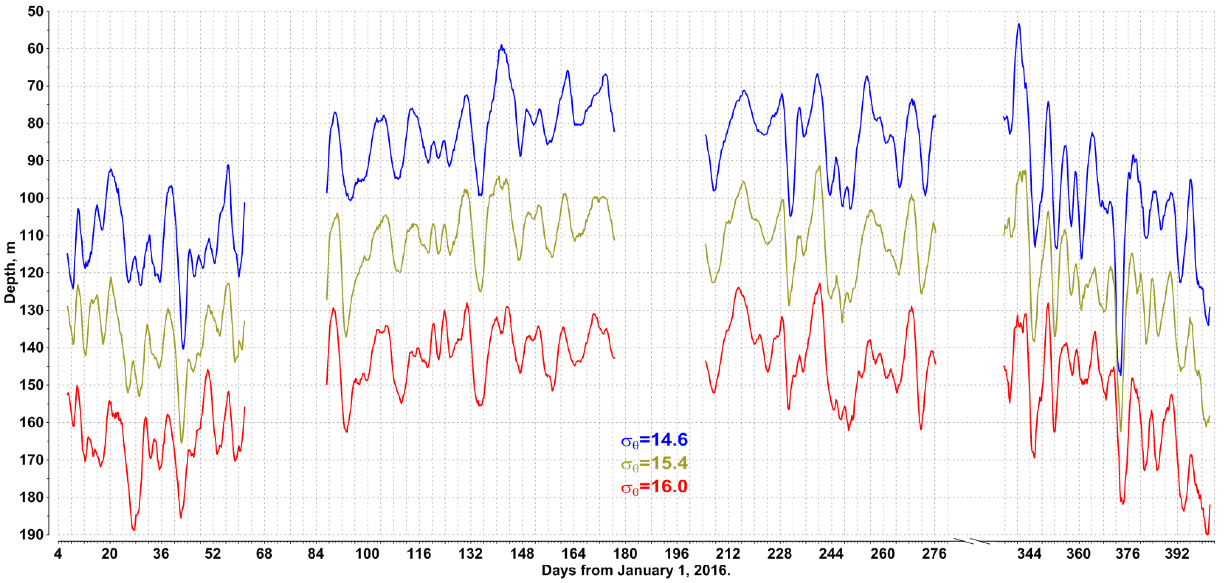
A general picture of isopycnal oscillations in the pycnocline (depth range from 60 to 200 m) for the period from January 2016 to February 2017 is shown in Figure 4. We chose three isopycnals, smoothed with a 2-day moving average: σθ = 14.6 kg/m3 (blue), 15.4 kg/m3 (olive), and 16.0 kg/m3 (red). The first of them represents the top of the pycnocline; the second—the nitrate maximum, usually found in the pycnocline at this density level [36]; and third—the redox zone (a thin anoxic layer between oxygenated water and deep water with hydrogen sulfide). The isopycnals demonstrated strong variability on a synoptic scale, with a typical period of 5–15 days, and some peak-to-peak values reached 50–60 m.
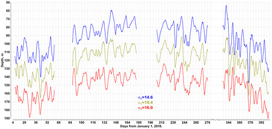
Figure 4.
Vertical dynamics of isopycnals (sigma–theta) from January 2016 to February 2017 on the continental slope, northeastern Black Sea, smoothed with 2-day moving average: 14.6 kg/m3 (blue), 15.4 kg/m3 (olive), and 16.0 kg/m3 (red).
An important point is that the oscillations of all three isopycnals were in-phase, with very similar amplitudes. Because of that, we used the “middle” isopycnal of 15.4 kg/m3 to demonstrate the correlation of density-level oscillations inside the pycnocline with the dynamics of current velocity (Figure 5).
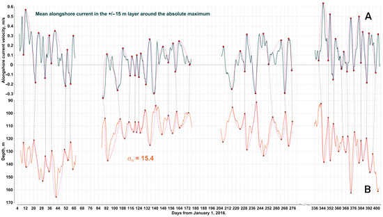
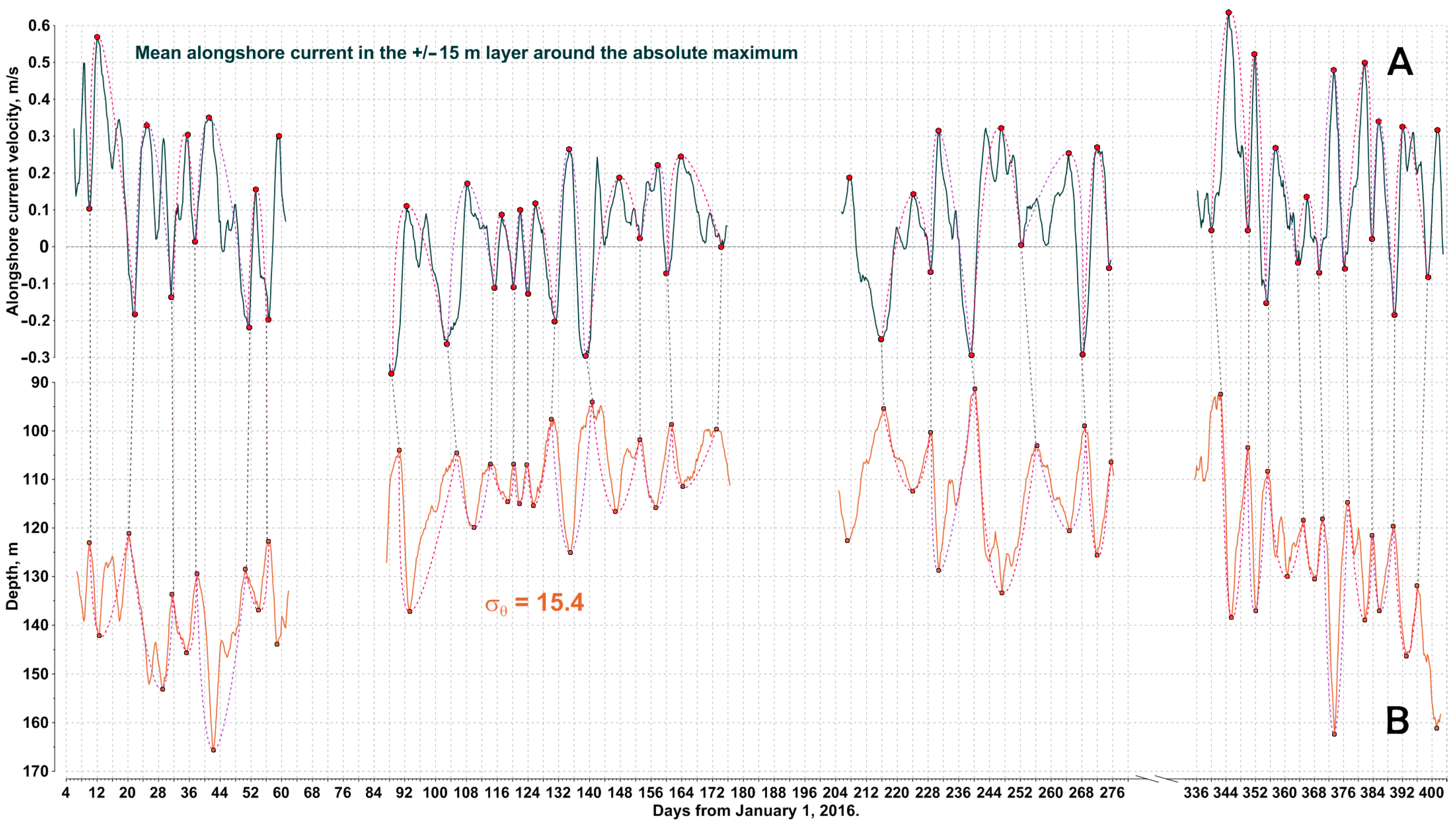
Figure 5.
Temporal variability of the alongshore current velocity parameter (A) and vertical dynamics of the isopycnal 15.4 kg/m3 (B) from January 2016 to February 2017 on the continental slope, northeastern Black Sea, smoothed with 2-day moving average. Red dots mark local extreme values. Vertical dashed lines connect local minimal values of the velocity parameter with the closest (in terms of time) minimal values of the isopycnal depth. Dotted splines mark full cycles of descend and ascend for the isopycnal and the corresponding oscillation cycles of the current velocity parameter.
Figure 5 demonstrates high correlation of the isopycnal vertical position with the alongshore current velocity parameter. An increase in the northwestern current (positive values) deepens the isopycnals, while that in the southeastern current (negative values) brings the isopycnals closer to the surface. However, it cannot be said that the velocity changes are ahead of the isopycnals: in about half the cases, the opposite is true.
An analysis of the full cycle of descend and ascend for the isopycnal 15.4 kg/m3 in Figure 5 provides the following statistics. The average period of the full cycle of descend and ascend was 8.9 days (range 3.5–16 days), with an average amplitude of 21.9 m (range 7.9–45.9 m). The amplitude was calculated as the difference between the point of maximal descend (maximal increase in case of velocity) and the average of the starting and ending values.
Corresponding statistics of the current velocity parameter are as follows. An average period of the full cycles “from a minimum to a minimum” was 9.3 days (range 3.7–16 days), with an average amplitude of 0.40 m/s (range 0.19–0.61 m/s). Apparently, average periods of the synoptic oscillations for the isopycnals and velocity parameter match each other fairly well.
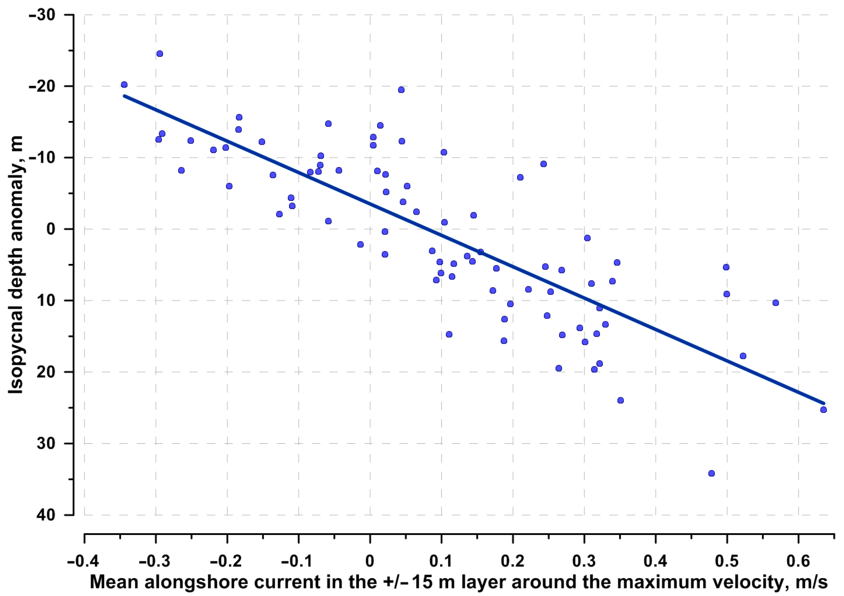
The seasonal signal was subtracted from the isopycnal position data (as described in the Section 2), and the respective local extreme values (red dots in Figure 5) of the isopycnal vertical oscillation and the alongshore current velocity parameter were plotted against each other (Figure 6) to determine the correlation between them. Our calculations show that there is a relatively high linear correlation between the synoptic anomalies of the isoline position (∆H) and the alongshore current velocity parameter (∆U).
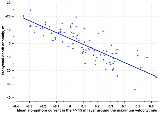
Figure 6.
Linear correlation between local extreme values of the current velocity parameter and the respective extreme values of the isopycnal 15.4 kg/m3 vertical position anomaly.
The equation of linear dependence of ∆H from ∆U, with a Pearson correlation coefficient R = 0.81, for the isopycnal 15.4 kg/m3 is as follows:
∆H = 43.9∆U − 3.51
For the isopycnals 14.6 and 16.0 kg/m3, the correlation dependence is almost the same, with Equations (6) and (7), correspondingly,
where R = 0.70 for (6) and R = 0.81 for (7).
∆H = 44.0∆U − 3.47,
∆H = 42.6∆U − 3.71,
A generalized formula for all three isopycnals, with R = 0.77, is as follows:
∆H = 43.5∆U − 3.57
To what extent these dependencies reflect geostrophic balance will be analyzed in Section 4.
3.2. Oscillations of Isotherms in the Seasonal Thermocline and Their Correlation with Alongshore Current Dynamics Based on Deep ADCP and Thermochain Data
In Figure 7, the isotherm dynamics, based on the deep thermochain data, are compared with the isopycnal dynamics, based on the Aqualog data. As it is seen in the figure, the synoptic oscillations of isotherms in a developed seasonal thermocline (late summer—autumn) are quasi-in-phase with the isopycnal oscillations in the pycnocline. Since the Aqualog and the deep thermochain were placed 2 km apart, it would be hard to expect a full synchronism between their measurements. Nevertheless, temporal inconsistencies between major oscillation peaks of the isotherms and isopycnals are generally less than one day.
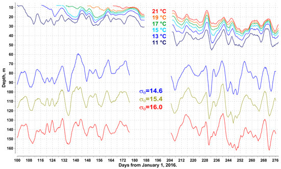
Figure 7.
Comparative dynamics of the isotherms in the upper layer, measured by the deep thermochain, and of the isopycnals in the pycnocline, measured by the Aqualog. The data shown represent the periods when both devices were working simultaneously and the seasonal thermocline was sufficiently developed.
Since the seasonal thermocline in the Black Sea only exists during a certain period (from April–May to November–December), higher-degree isotherms appear later in summer and are first to vanish when the cooling starts, while the lower-degree isotherms exist for a longer period and, thus, provide more data. The isotherms 10–11 °C in the lower part of the thermocline have the longest continuous existence, never vanishing during summer heating and the following autumn cooling. The synoptic oscillations of isotherms generally follow each other (Figure 7); so, the isotherm 11 °C was chosen to study the correlations between the alongshore current velocity and isopycnal dynamics.
The results are shown in Figure 8. Nearest local extreme values of the alongshore current velocity parameter and the vertical position of the isotherm 11 °C are connected with dashed lines. The tilting of these lines varies, in the same way as for the isopycnals (Figure 5). This would explain why a general correlation between the current velocity and isoline depth, which uses all the data and not just the connected extreme values, is rather poor.
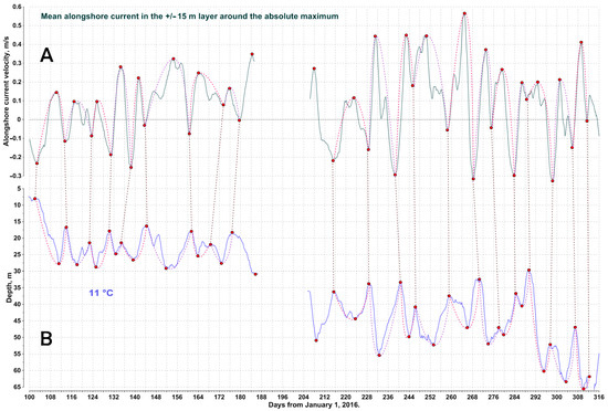
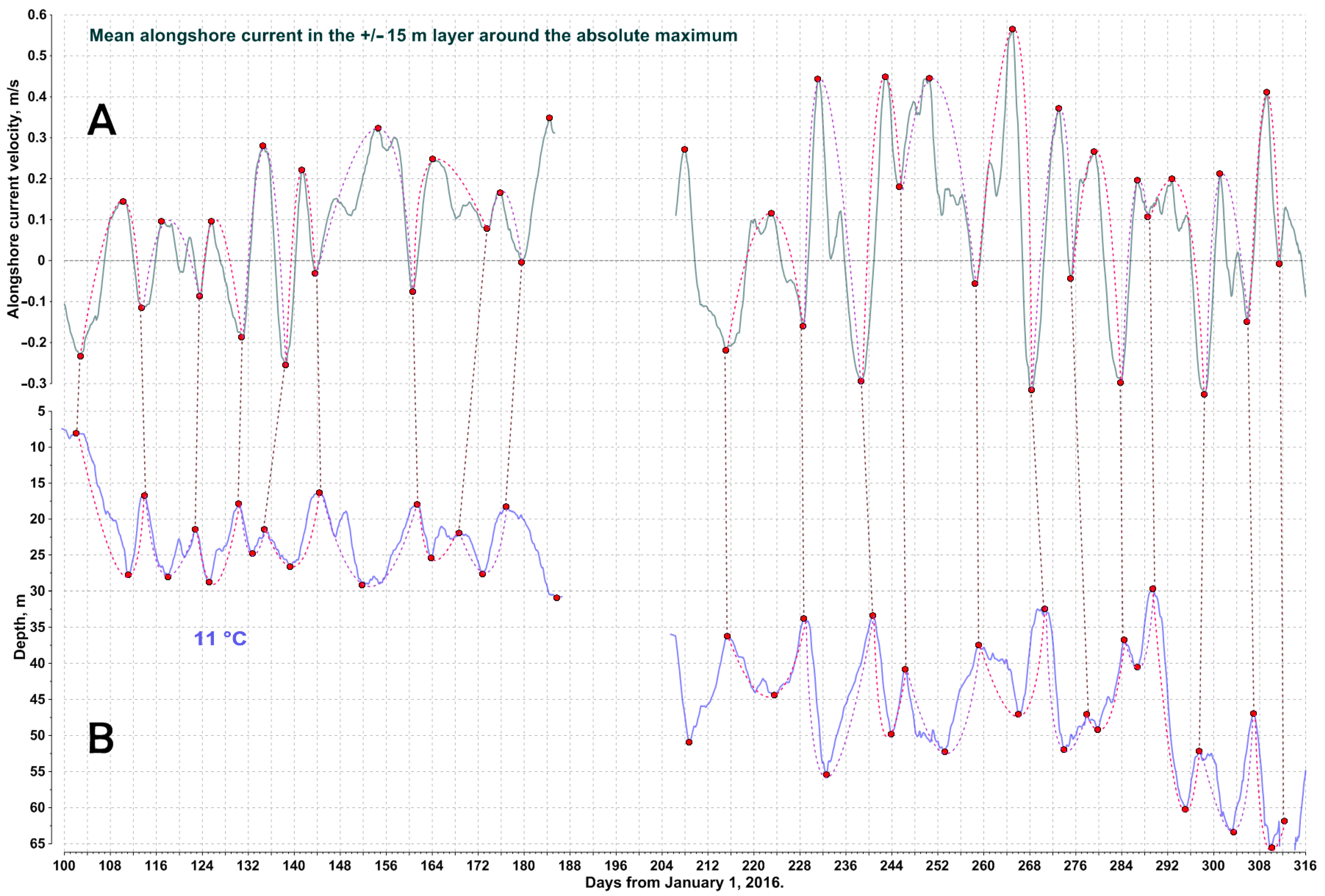
Figure 8.
Temporal variability of the alongshore current velocity parameter (A) and vertical dynamics of the isotherm 11 °C (B) in 2016, on the continental slope, northeastern Black Sea, smoothed with 2-day moving average. Red dots mark local extreme values. Vertical dashed lines connect local minimal values of the velocity parameter with the closest (in terms of time) minimal values of the isotherm depth. Dotted splines mark full cycles of descend and ascend for the isotherm and the corresponding oscillation cycles of current velocity.
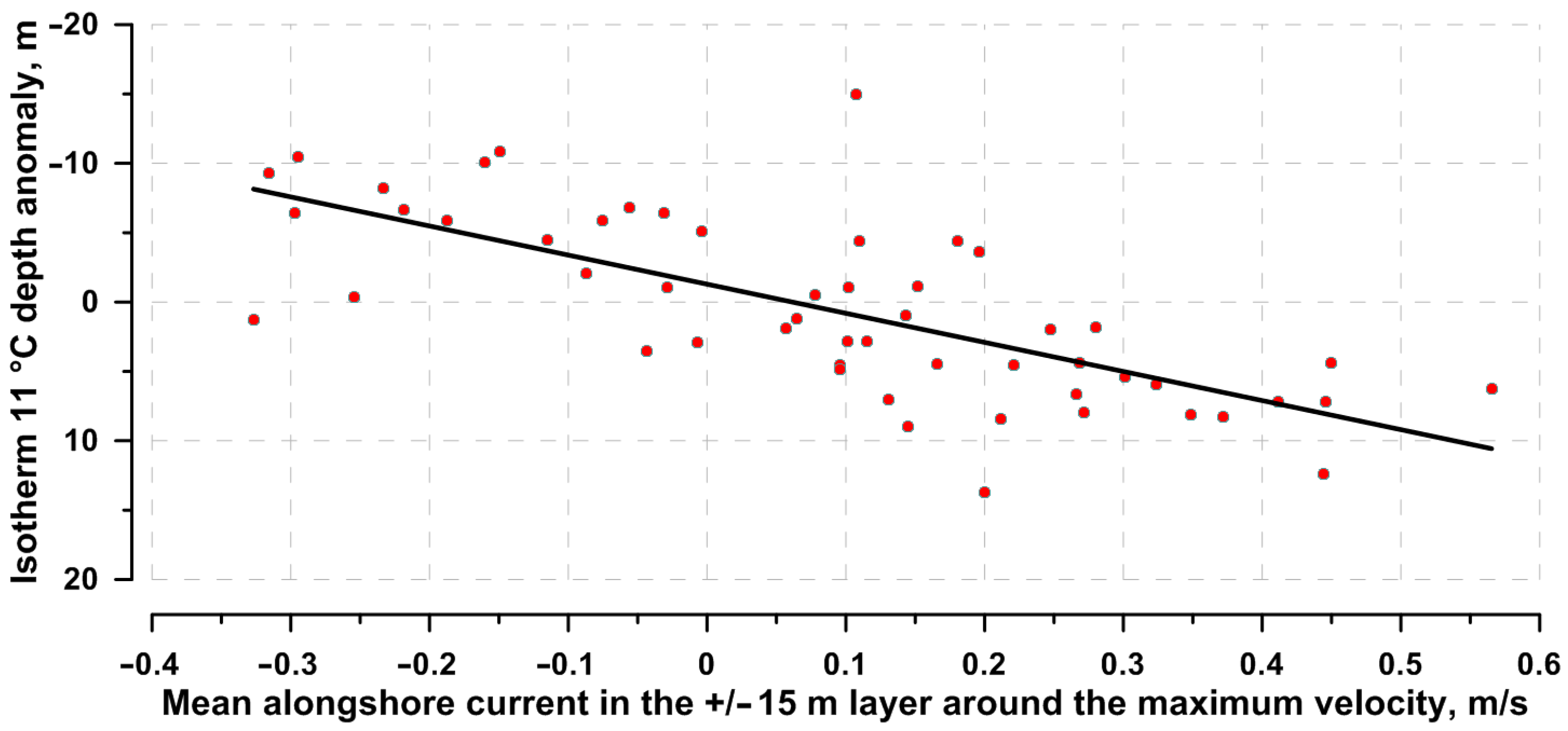
As seen in Figure 8, there is a good correlation between the current velocity oscillations, measured by the deep ADCP, and the dynamics of the isotherm 11 °C, measured by the deep thermochain. A linear correlation between the nearest extreme values of these parameters is shown in Figure 9. Apparently, their dynamics are closely interrelated.

Figure 9.
Linear correlation between local extreme values of the current velocity parameter and the respective extreme values of the isotherm 11 °C position anomaly.
The equation of linear dependence of ∆H from ∆U, with a Pearson correlation coefficient R = 0.81, for the isotherm 11 °C is as follows:
∆H = 21.0∆U − 1.29
Comparing the coefficients in (8) and (9), we can see that the isopycnal dynamics depend twice as much on the velocity oscillations than the isotherm dynamics. This difference will be discussed in the next section.
The statistics for the full cycles of descend and ascend for the isotherm 11 °C are as follows. An average period of the full cycle of descend and ascend was 9 days (range 3.3–17 days), with an average amplitude of 11.1 m (range 5.2–21.9 m). The corresponding statistics of the current velocity parameter showed an average period of 9.1 days (range 3.3–17 days) for the full cycle, with an average amplitude of 0.40 m/s (range 0.13–0.75 m/s).
3.3. Oscillations of Isotherms in the Seasonal Thermocline and Their Correlation with Alongshore Current Dynamics Based on Nearshore ADCP and Thermochain Data
Unlike the data from the Aqualog (the continental slope) or deep ADCP and thermochain (shelf edge), the data from the nearshore ADCP and thermochain station on the inner shelf (26 m depth) show significant variability (Figure 10). The thin surface layer was affected by wind and coastal inflow in a stronger way than the deep water of the outer shelf and continental slope. As seen in Figure 10, isotherms were constantly replacing each other, appearing and disappearing, and picking a temperature value that would exist in this layer for a long period was rather difficult. The most relevant option was the isotherm 14 °C, which continually existed in the measured data for 62 days.
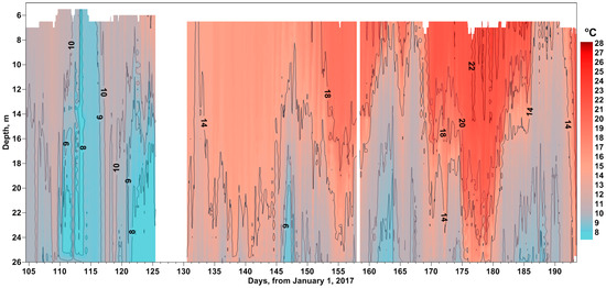
Figure 10.
General dynamics of temperature at the 26 m depth nearshore station during spring and summer of 2017 based on thermochain data.
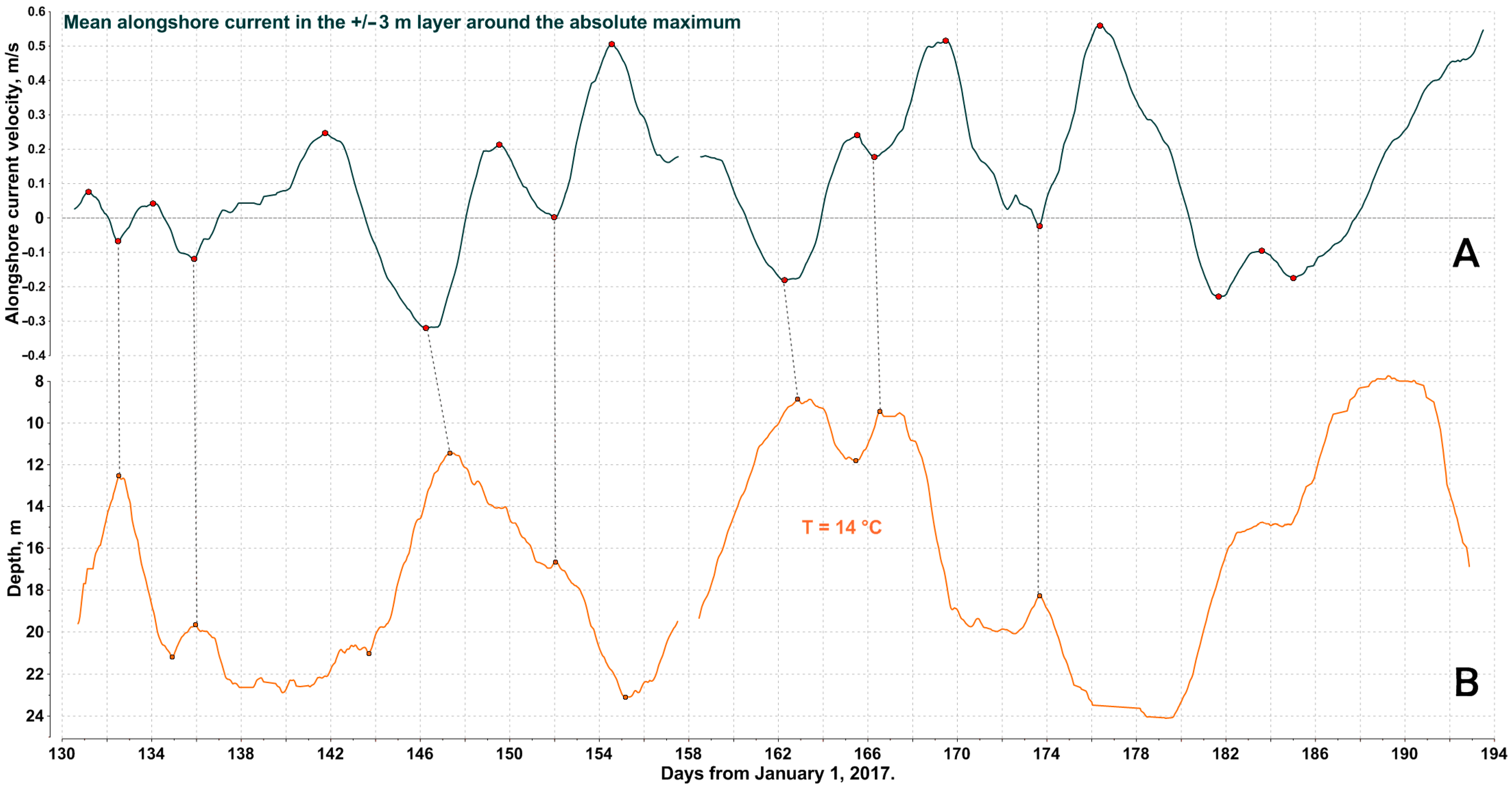
Oscillation diagrams of the alongshore current velocity parameter and the isotherm 14 °C are shown in Figure 11. As before, nearest local extreme values of both parameters are connected with dashed lines. As seen in Figure 11, there is still some correlation between the isotherm dynamics and the alongshore current velocity, although to a lesser extent than in the case of the deep stations. Unlike the deep stations, some local extreme values of current velocity have no obvious match in the isotherm vertical position.
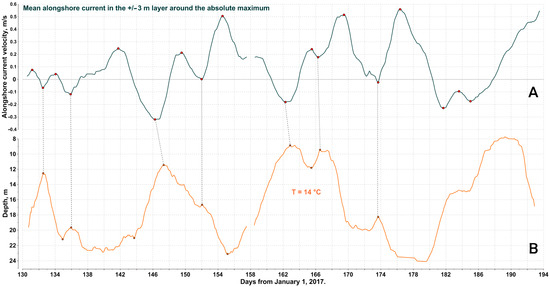
Figure 11.
Temporal variability of the alongshore current velocity parameter (A) and vertical dynamics of the isotherm 14 °C (B) in spring–summer 2017, at the 26 m depth nearshore station, smoothed with 2-day moving average. Red dots mark local extreme values. Vertical dashed lines connect local minimal values of the velocity parameter with the closest (in terms of time) minimal values of the isotherm depth.
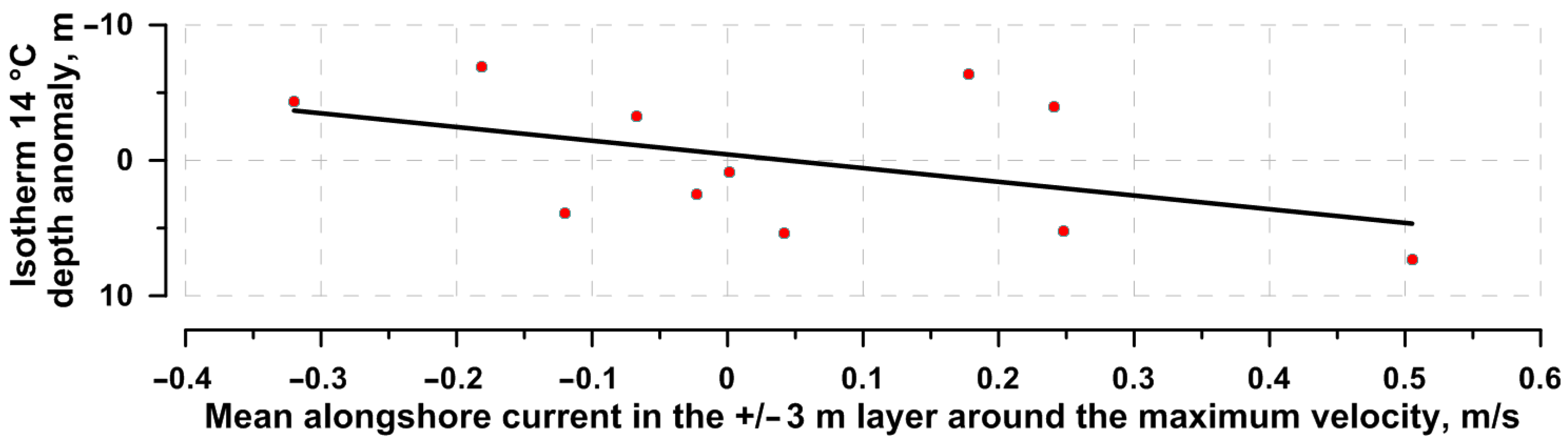
While the number of the connected local extreme values of the isotherm depth anomaly and the velocity parameter in this case is lacking, it is still possible to derive a certain linear correlation between them (Figure 12).
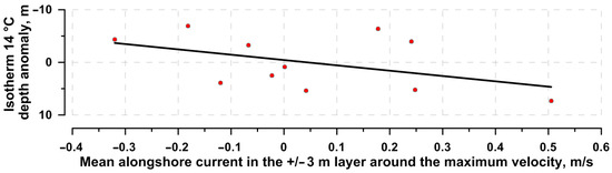
Figure 12.
Linear correlation between local extreme values of the current velocity parameter and the respective extreme values of the isopycnal 14 °C position anomaly.
The equation of linear dependence of ∆H from ∆U, with a Pearson correlation coefficient R = 0.46, for the isotherm 14 °C is as follows:
∆H = 10.1∆U − 0.44
Comparing the coefficients in (10) and (9) between the nearshore station and the one on the outer shelf, we can see that the nearshore isotherm dynamics depend half as much on the velocity oscillations than the isotherms measured at the deep station. This difference will also be discussed in the next section.
Despite the rather low correlation, a certain connection still exists between the alongshore current velocity dynamics and the isotherm’s vertical position, even in a shallow water layer heavily affected by perturbations of an ageostrophic nature.
Some statistical estimations can still be produced. An average period of the isotherm’s full descend and ascend cycle was 6.9 days (range 3.4–11.3 days), with an average amplitude of 6 m (range 2.7–10.3 m). The corresponding current velocity parameter had an average period of 6.6 days (range 3.4–10.3 days) for the full cycle, with an average amplitude of 0.38 m/s (range 0.11–0.69 m/s).
Therefore, there is a significant decrease in the average period and oscillation amplitude of the isotherm position at the nearshore station in comparison with the continental slope, while the average amplitude of the alongshore current velocity and its range remained almost the same.
4. Discussion
As was mentioned in the Section 1, the Black Sea shelf and continental slope have an overall downwelling circulation caused by the cyclonic Rim Current. The RC, however, is baroclinically unstable; its meandering produces mesoscale eddies, which slowly move along the coast following the RC direction. This leads to significant variations in the magnitude and direction of the alongshore current on a synoptic time scale [30], often resulting in local quasiperiodic upwellings and downwellings. The temporal variability of the vertical position of isopycnals in the pycnocline on the upper part of the continental slope (250 m depth), as well as isotherms in the seasonal thermocline on the outer (86 m) and inner shelf (26 m), has a pronounced oscillation mode with an average period of 9.1 days (range 3.3–17 days) for the outer shelf and continental slope, and 6.9 days (range 3.4–11.3 days) for the inner shelf. This mode has a distinct correlation with the magnitude and direction of the alongshore current velocity, confirming the concept of quasi-geostrophic adjustment.
To evaluate how far the registered oscillations of the isopycnals and isotherms comply with the conception of their geostrophic nature, let us substitute (1) into (3):
|∆H| = (H/g′)1/2∆U
First, we will apply (11) to the pycnocline. Here, |∆H| is the absolute value of isopycnal vertical shift, caused by a geostrophic current with a velocity difference ∆U in the pycnocline; g’ = g∆ρ/ρ is the reduced acceleration of gravity, where ∆ρ/ρ is a density difference in the pycnocline; and H is the average height of the upper layer, including the pycnocline. Substituting typical values, described in the Section 1, we obtain |∆H| ≈ 100∆U. The linear correlation coefficient for the isopycnal 15.4 kg/m3, however, presented in (5), is about 44. It is 2.3 times less than the number that follows from the pure geostrophic balance. Such a significant divergence could be, on one hand, a result of rather provisional parameters chosen to describe the problem; on the other hand, it could be caused by some ageostrophic factors (nonlinearity and friction), which can noticeably reduce a real vertical shift of the isopycnals in comparison with the pure geostrophic estimation. This issue requires further study.
The synoptic period of isotherm oscillations in the seasonal thermocline (based on the deep thermochain data) is roughly the same as the period of isopycnal oscillations in the pycnocline, and both of these oscillations are quasi-in-phase (Figure 7); this means that they are generated by the same mechanism. However, the average amplitude of the isotherm oscillations is 11.1 m, which is about two times less than the average amplitude of the isopycnal oscillations (21.9 m). According to (11), this difference is caused by the H/g′ ratio, which is four times less for the seasonal thermocline than for the pycnocline (assuming the thickness of the upper layer (i.e., the UML plus thermocline) H ≈ 50 m and the reduced acceleration of gravity g′= 2·10−2 m/s2, due to the temperature drop in the thermocline). At the same time, there was no difference between average amplitudes of the alongshore current velocity oscillations measured by the Aqualog and deep ADCP. In both cases, they had nearly the same value of about 0.4 m/s.
Although this estimation is quite crude, since the parameters of the thermocline vary significantly from month to month, the H/g′ ratio generally remains the same for the thermocline, at least during its formation period when the heat flux is directed downwards. This may be an indication that thermocline formation is a self-similar process; however, its patterns require additional study.
The abovementioned amplitude values of isotherm oscillation are based on the deep thermochain data. When it comes to the nearshore station, the average oscillation amplitude for the isotherms was only half as large (6 m against 11.1 m), most likely due to a bottom constraint that limits their vertical movement, and the average period of isotherm oscillations decreased as well (6.9 days against 9.1 days). In addition, the linear correlation between the isotherm vertical position and the alongshore current velocity parameter was significantly lower on the inner shelf (R = 0.46) compared with the continental slope (R = 0.81). Aside from the bottom constraint, wind impact and coastal inflow might also be the reasons behind the declined correlation since their effect increases towards the shore. Studies of wind impact and coastal inflow were put outside the scope of this paper since they are too complex and demand a separate investigation.
As mentioned above, nearshore upwellings, caused by the alongshore current reversal (geostrophic upwellings), usually do not bring thermocline water on the surface [31]. However, if they are further amplified with an appropriate wind stress, a full upwelling is a very likely event. It is quite possible that most full nearshore upwellings in the northeastern Black Sea are caused by joined effects of geostrophic and wind-driven upwellings.
Even if an upwelling is incomplete, it still brings the thermocline close to the surface. Followed by an intense wind force, the thermocline water is mixed into the UML, producing a cooling effect and enriching the upper layer with nutrients [3]. Additional nutrients will also enter the photic layer from the pycnocline, where the nitrate maximum is located at the isopycnal level of 15.4 kg/m3. As mentioned in the Section 3, the average amplitude of vertical oscillations of this isopycnal exceeds 20 m; this is a significant value, comprising about 15–20% of the total average depth of this isopycnal in the slope area of the Black Sea. Combined with a large vertical turbulent exchange coefficient in the layers with a high vertical velocity shear (such as the pycnocline) [37], the total inflow of nitrates into the photic layer can increase significantly. This aspect still needs further research.
High-frequency oscillations of the lower boundary of the oxygenated zone (σθ = 15.85 kg/m3) can have a serious impact on benthos communities [38,39], leading to ecosystem instability and degradation. However, no clear evidence of such an effect on benthos was found on the continental slope of the northeastern Black Sea. According to the present data [40], based on continuous 2-month-long observations, a boundary between different biological communities at the depth of 80–150 m is determined only by the total duration of hypoxia. A complete transfer from a depleted ecosystem to an ephemeral one only occurs if, during the mentioned 2-month observation period, the total hypoxia duration exceeds 1.5 months.
5. Conclusions
- Based on the long-term measurements of current velocity and CTD data by bottom-anchored stations on the shelf and upper part of the continental slope of the northeastern Black Sea, it was found that vertical oscillations of isopycnals in the permanent pycnocline and isotherms in the seasonal thermocline (upwellings and downwellings) on a synoptic time scale (5–15 days) are caused primarily by geostrophic adjustment of density and velocity fields. At the same time, quasi-geostrophic oscillations of the alongshore current velocity in the shelf–slope area are caused by the baroclinic instability of the Rim Current, its meandering, and the formation of mesoscale eddies.
- Statistically significant linear correlations of vertical oscillations of isotherms and isopycnals from the alongshore current velocity were discovered, which make it possible to estimate the magnitude of upwellings and downwellings in the shelf–slope area of the northeastern Black Sea using long-term measurements of current velocity profiles.
- Typical periods of synoptic oscillations of isopycnals in the pycnocline on the upper part of continental slope (250 m depth) are about 9 days, and their typical amplitudes are 22 m. Oscillations of isotherms in the seasonal thermocline on the outer shelf (86 m depth) have almost the same period but the average amplitude is half as large. On the inner shelf (26 m depth), the average isotherm oscillation amplitude and period are even smaller: about 6 m and 7 days, respectively, due to ageostrophic effects.
Author Contributions
Conceptualization, O.I.P., K.P.S. and A.G.Z.; data curation, O.I.P. and V.V.O.; formal analysis, O.I.P. and A.G.Z.; funding acquisition, A.G.Z.; methodology, O.I.P., V.V.O., K.P.S. and A.G.Z.; project administration, A.G.Z.; resources, V.V.O. and K.P.S.; writing—original draft, O.I.P. and A.G.Z. All authors have read and agreed to the published version of the manuscript.
Funding
This work was funded by the Russian Science Foundation, grant NO. 23-17-00056 (https://rscf.ru/project/23-17-00056/, (accessed on 16 August 2023)), with partial support from the frameworks of state assignment FMWE-2021-0002 (K.P.S., A.G.Z.) and FMWE-2021-0013 (O.I.P., V.V.O.).
Institutional Review Board Statement
Not applicable.
Informed Consent Statement
Not applicable.
Data Availability Statement
Not applicable.
Acknowledgments
The authors are thankful to S.V. Stanichny for a satellite image of mesoscale eddies in the studied area.
Conflicts of Interest
The authors declare no conflict of interest.
References
- Ekman, V.W. On the influence of the Earth’s rotation on ocean-currents. Ark. Foer Mat. Astron. Och Fys. 1905, 2, 1–53. [Google Scholar]
- Gill, A.E.; Clarke, A.J. Wind-induced upwelling, coastal currents, and sea-level changes. Deep-Sea Res. 1974, 21, 325–345. [Google Scholar] [CrossRef]
- Yentsch, C.S. The influence of geostrophy on primary production. Tethys 1974, 6, 111–118. [Google Scholar]
- Kämpf, J.; Chapman, P. Upwelling Systems of the World; Springer International Publishing: Cham, Switzerland, 2016; p. 433. [Google Scholar]
- Stanichnaya, R.R.; Stanichny, S.V. Black Sea upwellings. Sovrem. Probl. Distantsionnogo Zondirovaniya Zemli Iz Kosmosa 2021, 18, 195–207. (In Russian) [Google Scholar] [CrossRef]
- Gawarkiewicz, G.; Korotaev, G.; Stanichny, S.; Repetin, L.; Soloviev, D. Synoptic upwelling and cross-shelf transport processes along the Crimean coast of the Black Sea. Cont. Shelf Res. 1999, 19, 977–1005. [Google Scholar] [CrossRef]
- Zhurbas, V.; Oh, I.S.; Park, T. Formation and decay of a longshore baroclinic jet associated with transient coastal upwelling and downwelling: A numerical study with applications to the Baltic Sea. J. Geophys. Res. 2006, 111, C04014. [Google Scholar] [CrossRef]
- García-Reyes, M.; Sydeman, W.J.; Schoeman, D.S.; Rykaczewski, R.R.; Black, B.A.; Smit, A.J.; Bograd, S.J. Under Pressure: Climate Change, Upwelling, and Eastern Boundary Upwelling Ecosystems. Front. Mar. Sci. 2015, 2, 109. [Google Scholar] [CrossRef]
- Sur, H.I.; Ozsoy, E.; Ilyin, Y.P.; Unluata, U. Coastal/deep ocean interactions in the Black Sea and their ecological/environmental impacts. J. Mar. Syst. 1996, 7, 293–320. [Google Scholar] [CrossRef]
- Freon, P.; Barrange, M.; Aristegni, J. Eastern boundary upwelling ecosystems: Integrative and comparative approaches. Prog. Oceanogr. 2009, 83, 1–14. [Google Scholar] [CrossRef]
- Blatov, A.S.; Bulgakov, N.P.; Ivanov, V.A.; Kosarev, A.N.; Tujilkin, V.S. Variability of Hydrophysical Fields in the Black Sea; Gidrometeoizdat: Leningrad, Russia, 1984; p. 240. (In Russian) [Google Scholar]
- Oguz, T.; La Violette, P.E.; Unluata, U. The upper layer circulation of the Black Sea: Its variability as inferred from hydrographic and satellite observations. J. Geophys. Res. Oceans 1992, 97, 12569–12584. [Google Scholar] [CrossRef]
- Besiktepe, S.T.; Lozano, C.J.; Robinson, A.R. On the summer mesoscale variability of the Black Sea. J. Mar. Res. 2001, 59, 475–515. [Google Scholar] [CrossRef]
- Titov, V.B. Circulation and vertical structure of currents in the eastern part of the Black Sea. Oceanology 1980, 20, 425–431. (In Russian) [Google Scholar]
- Oguz, T.; Latun, V.S.; Latif, M.A.; Vladimirov, V.V.; Sur, H.I.; Markov, A.A.; Özsoy, E.; Kotovshchinnikov, B.B.; Eremeyev, V.V.; Ünlüata, Ü. Circulation in the surface and intermediate layers of the Black Sea. Deep Sea Res. I Ocean. Res. Papers 1993, 40, 1597–1612. [Google Scholar] [CrossRef]
- Oguz, T.; Besiktepe, S. Observations on the Rim Current structure, CIW formation and transport in the western Black Sea. Deep Sea Res. I Ocean. Res. Papers 1999, 46, 1733–1753. [Google Scholar] [CrossRef]
- Sapozhnikov, V.V. Biohydrochemical barrier along the border of shelf waters of the Black Sea. Oceanology 1991, 31, 417–423. [Google Scholar]
- Zhurbas, V.M.; Zatsepin, A.G.; Grigor’eva, Y.V.; Eremeev, V.N.; Kremenetsky, V.V.; Motyzhev, S.V.; Poyarkov, S.G.; Poulain, P.M.; Stanichny, S.V.; Soloviev, D.M. Water Circulation and Characteristics of Currents of Different Scales in the Upper Layer of the Black Sea from Drifter Data. Oceanology 2004, 44, 30–43. [Google Scholar]
- Stanev, E.V. On the mechanisms of the Black Sea circulation. Earth-Sci. Rev. 1990, 28, 285–319. [Google Scholar] [CrossRef]
- Korotaev, G.; Oguz, T.; Nikiforov, A.; Koblinsky, C. Seasonal, interannual, and mesoscale variability of the Black Sea upper layer circulation derived from altimeter data. J. Geophys. Res. 2003, 108, 3122. [Google Scholar] [CrossRef]
- Sur, H.I.; Ozsoy, E.; Unluata, U. Boundary current instabilities, upwelling, shelf mixing and eutrophication processes in the Black Sea. Prog. Oceanogr. 1994, 33, 249–302. [Google Scholar] [CrossRef]
- Titov, V.B. Characteristics of the Main Black Sea Current and near-shore anticyclonic eddies in the Russian sector of the Black Sea. Oceanology 2002, 42, 637–645. [Google Scholar]
- Sokolova, E.; Stanev, E.V.; Yakubenko, V.; Ovchinnikov, I.; Kos’yan, R. Synoptic variability in the Black Sea. Analysis of hydrographic survey and altimeter data. J. Mar. Syst. 2001, 31, 45–63. [Google Scholar] [CrossRef]
- Staneva, J.; Dietrich, D.; Stanev, E.; Bowman, M. Rim Current and coastal eddy mechanisms in an eddy resolving general circulation model. J. Mar. Syst. 2001, 31, 137–158. [Google Scholar] [CrossRef]
- Ginzburg, A.I.; Kostyanoy, A.G.; Soloviev, D.M.; Stanichny, S.V. Satellite monitoring of eddies and jets in the northeastern Black Sea. Mapp. Sci. Remote Sens. 2001, 38, 21–35. [Google Scholar] [CrossRef]
- Ovchinnikov, I.M.; Titov, V.B. Anticyclonic vorticity of the currents in the coastal zone of the Black Sea. Proc. USSR Acad. Sci. 1990, 314, 1236–1239. (In Russian) [Google Scholar]
- Demyshev, S.G.; Dymova, O.A. Numerical analysis of the mesoscale features of circulation in the Black Sea coastal zone. Izv. Atmos. Ocean. Phys. 2013, 49, 603–610. [Google Scholar] [CrossRef]
- Korotenko, K.; Osadchiev, A.; Melnikov, V. Mesoscale Eddies in the Black Sea and Their Impact on River Plumes: Numerical Modeling and Satellite Observations. Remote Sens. 2022, 14, 4149. [Google Scholar] [CrossRef]
- Morozov, A.N.; Zatsepin, A.G.; Kuklev, S.B.; Ostrovskii, A.G.; Fedorov, S.V. Vertical structure of the currents in upper part of the Black Sea continental slope near Gelendzhik city. Izv. Atmos. Ocean. Phys. 2017, 6, 718–727. [Google Scholar]
- Zatsepin, A.G.; Ostrovskii, A.G.; Kremenetskiy, V.V.; Piotukh, V.B.; Kuklev, S.B.; Moskalenko, L.V.; Podymov, O.I.; Baranov, V.I.; Korzh, A.O.; Stanichny, S.V. On the nature of short-period oscillations of the main Black Sea pycnocline, submesoscale eddies, and response of the marine environment to the catastrophic shower of 2012. Izv. Atmos. Ocean. Phys. 2013, 49, 659–673. [Google Scholar] [CrossRef]
- Silvestrova, K.P.; Zatsepin, A.G.; Myslenkov, S.A. Coastal upwelling in the Gelendzhik area of the Black Sea: Effect of wind and dynamics. Oceanology 2017, 57, 469–477. [Google Scholar] [CrossRef]
- Abramov, A.A.; Blatov, A.S.; Ul’yanova, V.I. Barotropic-Baroclinic Instability of the Main Black Sea Flow and Eddy Formation in the Black Sea. Izv. Akad. Nauk. SSSR Fiz. Atmos. I Okeana 1981, 17, 974–981. (In Russian) [Google Scholar]
- Kubryakov, A.A.; Stanichny, S.V. Mesoscale eddies in the Black Sea from satellite altimetry data. Oceanology 2015, 55, 56–67. [Google Scholar] [CrossRef]
- Akima, H. Algorithm 526: Bivariate Interpolation and Smooth Surface Fitting for Irregularly Distributed Data Points. ACM Trans. Math. Softw. 1978, 4, 160–164. [Google Scholar] [CrossRef]
- Zatsepin, A.G.; Piotouh, V.B.; Korzh, A.O.; Kukleva, O.N.; Soloviev, D.M. Variability of currents in the coastal zone of the Black Sea from long-term measurements with a bottom mounted ADCP. Oceanology 2012, 52, 579–592. [Google Scholar] [CrossRef]
- Murray, J.W.; Codispoti, L.A.; Friederich, G.E. The suboxic zone in the Black Sea. In Aquatic Chemistry: Interfacial and Interspecies Process; Advances in Chemistry Series No. 244; Huang, C.P., O’Melia, R., Morgan, J.J., Eds.; American Chemical Society: Washington, DC, USA, 1995; pp. 157–176. ISBN 0-8412-2921-X. [Google Scholar]
- Morozov, A.N.; Lemeshko, E.M.; Shutov, S.A.; Zima, V.V.; Deryushkin, D.V. Structure of the Black Sea currents based on the results of the ladcp observations in 2004–2014. Phys. Ocean. 2017, 1, 25–40. [Google Scholar]
- Chu, J.W.F.; Curkan, C.; Tunnicliffe, V. Drivers of temporal beta diversity of a benthic community in a seasonally hypoxic fjord. R. Soc. Open Sci. 2018, 5, 172284. [Google Scholar] [CrossRef] [PubMed]
- Villnäs, A.; Norkko, J.; Hietanen, S.; Josefson, A.; Lukkari, K.; Norkko, A. The role of recurrent disturbances for ecosystem multifunctionality. Ecology 2013, 94, 2275–2287. [Google Scholar] [CrossRef] [PubMed]
- Kolyuchkina, G.A.; Syomin, V.L.; Simakova, U.V.; Sergeeva, N.G.; Ananiev, R.A.; Dmitrevsky, N.N.; Lyubimov, I.V.; Zenina, M.A.; Podymov, O.I.; Basin, A.B.; et al. Benthic community structure near the margin of the oxic zone: A case study on the Black Sea. J. Mar. Syst. 2022, 227, 103691. [Google Scholar] [CrossRef]


Disclaimer/Publisher’s Note: The statements, opinions and data contained in all publications are solely those of the individual author(s) and contributor(s) and not of MDPI and/or the editor(s). MDPI and/or the editor(s) disclaim responsibility for any injury to people or property resulting from any ideas, methods, instructions or products referred to in the content. |
© 2023 by the authors. Licensee MDPI, Basel, Switzerland. This article is an open access article distributed under the terms and conditions of the Creative Commons Attribution (CC BY) license (https://creativecommons.org/licenses/by/4.0/).