1. Introduction
The harsh underwater environment presents numerous challenges to manned operations. Consequently, many applications are switching to underwater unmanned platforms, such as autonomous underwater vehicles (AUVs) or remote control vehicles (rovs), to execute tasks that are difficult and dangerous for humans to undertake, thereby facilitating underwater applications, such as data collections in underwater wireless sensor networks (UWSNs) [
1,
2], target detection and tracking [
3], and underwater pipeline monitoring [
4].
There is a need to track the vehicles’ status, particularly the location and velocity, constantly. For example, during an operation, the vehicle’s real-time status needs to be readily available to the vehicle owner and operator to know where the vehicle is and where it is going. In addition, this information is also important to the vehicle’s navigation system when the calibration of the inertial sensor is needed [
5,
6,
7]. In terrestrial environments, the GNSS (Global Navigation Satellite System) signal can be used to eliminate the accumulated error of the inertial sensor. However, it is not the case underwater, where the GNSS signals do not travel well. Therefore, the location and velocity estimation have to be obtained in a different manner.
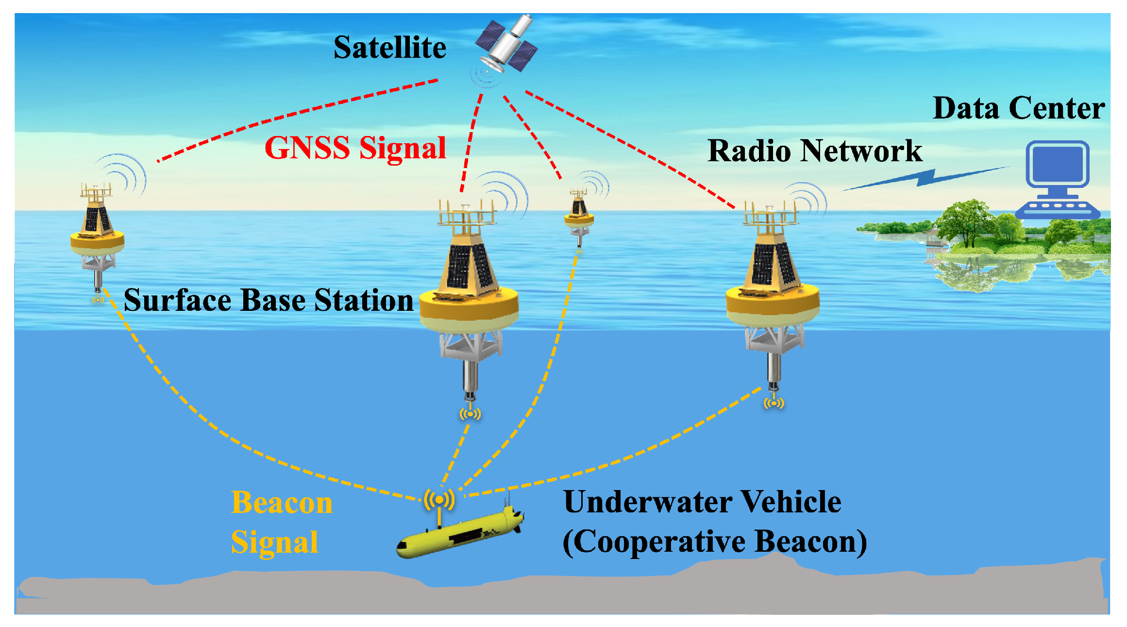
In this paper, we present a distributed intelligent buoy system (DIBS) for tracking the underwater vehicle’s location and velocity. We explain the design of such a system from three aspects. The first aspect concerns the design of system architecture, its components, and the relationships among them. The second aspect involves the signal processing methods employed by the system. In this aspect, we primarily focus on the techniques for signal detection, time of arrival (ToA) estimation, and the Doppler scaling factor estimation from the signal. And the final aspect is about how the results of signal processing are leveraged for estimating the location and velocity of underwater vehicle.
Within DIBS, there are three main components: the cooperative beacon (CB), the surface base station (SBS), and the data center (DC). Each of the vehicles in the system carries a beacon, which actively and periodically broadcasts the beacon signal. A set of SBSs passively listen to the beacon signal. Upon receiving, the SBS performs estimation of ToA and Doppler scaling factor. These measurements are then forwarded to the DC. Finally, the DC gathers the measurements obtained from all SBSs and estimates the vehicle’s location and velocity.
Due to the consideration of accuracy, we employ ranging-based localization and Doppler-based velocity estimation, requiring signal processing methods to estimate the ToA and the Doppler scaling factor about the received signal. To facilitate the estimation, a beacon signal comprising dual-hyperbolic-frequency-modulated (HFM) waveform and an OFDM symbol with cyclic prefix (CP) is employed. Based on this signal, the ToA of beacon signal is effectively estimated by using the Page test statistic. Additionally, estimation of Doppler scaling factor can be conveniently achieved by leveraging the null subcarriers within the CP-OFDM symbol. In addition to its use for estimating the ToA and Doppler scale, there are several other reasons that contribute to our employment of this beacon signal. Firstly, the underwater environment is prone to impulsive noise, leading to false alarms which result in anomalous ranging data. To address this, we employ a dual-HFM structure, with the second HFM acting as a redundancy. Additionally, the CP-OFDM symbol transmitted after the dual-HFM structure ensures that only signals with a matched pattern are considered as beacon signals, further mitigating false alarms. Finally, in centralized localization, when the maximum propagation delay is longer than the period between two successive beacon signals, it is hard to decide which set of measurements belongs to the same epoch. Thus, further processing needs to be performed on the measurements. To enhance efficiency, we modulate the epoch number into the CP-OFDM symbol, allowing the DC to determine which set of measurements belong to the same epoch in a more straightforward manner.
With the determined ToA and Doppler scaling factor from the SBS, localization and velocity estimation are performed at DC. We form least squares estimators for underwater vehicle location and velocity. The location is estimated using a time difference of arrival (TDoA) method, while the velocity is estimated by utilizing the Doppler scaling factors.
The main contributions of this paper are:
In this paper, we present the design and implementation of a self-contained, fully integrated and practical solution for underwater vehicle’s location and velocity. Detailed information about the overall architecture of the system, system components, the functionality definitions of each component, the relationships and interfaces between them, as well as the underlying signal processing and mobility estimation methods are given.
Through the employment of a signal comprising a dual-HFM and a CP-OFDM symbol, we achieve efficient ToA and Doppler scale estimation while reducing the false alarms. Additionally, essential information is modulated in the CP-OFDM symbol, thereby enhancing the efficiency of location and velocity estimation process.
To verify the effectiveness of our purposed system, experiments are conducted at Dapeng Bay, Shenzhen. Within the test area, four SBSs are deployed, which forms a four-grid square topology. The experiment results are compared with the ground truth obtained from the GNSS receiver. And, the results show the feasibility and effectiveness of our proposed system.
The rest of the paper is arranged as follows:
Section 2 reviews the existing works related to the design of remote tracking systems for the underwater vehicle mobility state.
Section 3 outlines the system architecture, while
Section 4 provides a detailed description of our signal processing and mobility state estimation methods.
Section 5 presents our field test results, and in
Section 6, we draw our conclusions.
2. Related Work
DIBS is designed for underwater vehicle mobility state estimation, where the mobility state includes location and velocity, thus resulting in related research that can be broadly categorized into two topics: location estimation and velocity estimation. Accordingly, the review of relevant work is split into two parts, each focused on either location or velocity estimation.
Location estimation. The localization of underwater vehicle can be accomplished with two kinds of methods: range-based and non-range-based [
8]. The focus of this paper is the range-based approach. Under such an approach, a correlation is established between the measured range and the underwater vehicle’s location. Two types of algorithms can be used to resolve the location of underwater vehicle, namely the iterative-based algorithm [
9] and the closed-form algorithm [
10]. The iterative-based algorithm resolves underwater vehicle’s location as a nonlinear least squares problem and is solved using an iterative approach. Conversely, the closed-form algorithm links measurements directly to the underwater vehicle’s location through a set of equations.
As stated in [
11], underwater localization systems are typically classified into ultra-short baseline, short baseline, and long baseline. The long baseline system, which utilizes multiple base stations to provide redundant measurements and ensure system reliability, generally offers superior localization accuracy and wider area coverage. Long baseline systems can be deployed on the seafloor or carried by buoys, depending on the intended application. It can be challenging to calibrate the exact geodetic coordinates of base stations deployed underwater. To address this, a common practice is to continually ranging the base stations using vessels equipped with GPS and hydrophones at various locations [
12].
Given its superior accuracy and coverage, the long baseline system is deemed more appropriate for establishing the desired system. Considering the need for flexible deployment and to avoid intricate calibration processes, the SBS-based long baseline system is a preferred choice. The GPS intelligent buoy (GIB) system [
13,
14] is a design that features surface buoys which serve as a platform carrying base station.The buoys are commonly equipped with GPS receivers, thus their precise location can be acquired. Therefore, underwater nodes can determine their geodetic coordinates by performing localization with surface buoys as reference points. The GIB system’s flexibility allows it for easy deployment to different areas.
Apart from the works related to GIB, which give a broad overview about the surface-buoy-based localization system, many research studies which focus on how to perform precise localization with the SBS have been conducted. In the system proposed in [
15], a set-membership approach is utilized to localize underwater vehicles. Ranging results between the base station and the underwater vehicle are used to determine a set of ring-shaped regions centered on the base station. The intersection points of the rings form a rectangle whose interior represents the possible location of the underwater vehicle. As the number of base stations increases, the iterative reduction of the possible location of the underwater vehicle results in a computationally intensive method.
In [
16], the author propose a GIB-based localization system for underwater vehicles in which vehicles synchronize with the base station and periodically transmit beacon signals. The system employs the ToA method to localize underwater vehicles while encoding depth information in the two consecutive pulse intervals of the signal.
Passive localization methods based on the TDoA are proposed in [
17,
18]. In [
17], during localization, the number of measurements may not be sufficient to meet localization requirements due to the influence of acoustic channels. To overcome this, the authors proposed two modified methods, whereby the first employs buffered messages to construct a virtual node to predict virtual arrival times, and the second utilizes motion information and an extended Kalman filter (EKF) to estimate the location of the underwater vehicle. In [
18], a three-stage method for target localization is proposed, where the non-linear equations of localization are transformed into the pseudolinear equations by introducing nuisance variables, and the estimated location of the unknown source is further optimized by improving the estimation accuracy of the interference variable. A similar system is proposed in [
19], in which an EKF method is employed to predict the motion of the underwater vehicle. Apart from directly ranging, the work in [
20] proposes a received signal-strength-indication (RSSI)-based method for indoor localization scenarios. A least-squares curve fitting is designed to estimate the critical radio propagation parameters of the transmit power and path loss exponent. Then, the resulting signal strength is converted to range, and a trilateration method is adopted for localization. Finally, a Bayesian filter is applied to improve the localization accuracy.
Apart from the localization method proposed for different scenarios, researches have been conducted to deal with the ranging noise and range ambiguity problem. To deal with range measurements that are degraded by noise and outliers, a method is proposed which applies graph partitioning for range-measurement outlier rejection in [
21], aiming to aid the navigation of AUVs. The range ambiguity problem occurs when the period between successive beacon signals is shorter than the maximum propagation delay of the beacon signal to a distant surface buoy. To resolve the ambiguity, a method is proposed that utilized a designed OFDM waveform to mitigate the range ambiguities dedicated to a synthetic-aperture radar case in [
22].
Velocity estimation. The remote tracking of an underwater vehicle’s velocity can be achieved with the help of Doppler scaling factor estimation. Prior studies on Doppler scaling factor estimation can be found in [
23,
24]. Studies like [
25,
26] have proposed velocity estimation methods that rely on estimated Doppler scaling factors.
To estimated Doppler scaling factors in underwater multicarrier systems, methods have been proposed which rely on the scaling in time of transmitted signals and the inherent characteristics of the OFDM symbol [
23,
24]. In [
23], a Doppler scale estimation technique that utilizes the null subcarrier of a CP-OFDM symbol is proposed. The proposed method estimates the Doppler scaling factor through a two-step algorithm. The first step involves resampling the received signal, which compensates the majority of Doppler shift. The resulting signal can be considered as affected by frequency-independent Doppler shift. In the second step, a channel frequency offset (CFO) estimation is conducted on the output signal in the first step to make more accurate compensation. In [
24], a Doppler estimation method based on the embedded repetition pattern is proposed. The transmitted signal contains a repetition pattern that may undergo changes due to unknown factor(s) when transmitted through a channel affected by the Doppler effect and consequently, the repetition period changed. A filter bank with each branch having a possible value of changed period is proposed. The branch with the highest correlation metric with the incoming signal is regarded as the best match.
Upon the estimation of Doppler scaling factors, velocity estimation can be conducted accordingly. A GIB-based system is proposed in [
25], which uses a closed-form algorithm to estimate the underwater vehicle’s velocity with at least two base stations. The input to the algorithm consists of a Doppler shift measurement of the received signal and information about the location of the base stations. However, this paper does not mention the signal processing method on how to extract the Doppler scaling factor on which the accuracy of the speed estimation heavily depends. Additionally, the experimental results do not report the algorithm’s performance at different signal-to-noise ratios.
Apart from utilizing the SBS, in [
26], a multiple AUV-assisted velocity estimation method is proposed that combines the location and velocity information of at least three neighboring AUVs and the radial velocity produced from the estimation of Doppler scaling factor. The estimation process consists of a data acquisition phase and a closed-form algorithm that determines underwater vehicle’s velocity in three dimensions.
In addition to the aforementioned works, there are some studies that estimate underwater vehicle location and velocity simultaneously. As proposed in [
27], an algebraic solution for target location and velocity is given, which is shown to achieve the Cramér–Rao lower bound for Gaussian TDoA and FDoA noise at moderate noise level before the thresholding effect occurs. In [
28], a closed-form estimator of target location and velocity is proposed, as in [
27]. The accuracy of the estimation achieves the Cramér–Rao lower bound at a sufficiently high noise level before the threshold effect occurs.
To summarize, previous works on system designs based on surface base stations are not directly applicable to our intended system because they lack specific methods for location and velocity estimation. Furthermore, studies on location and velocity estimation either focus on only one aspect or neglect the signal processing methods at the physical layer and the design considerations for achieving a system. Therefore, this paper takes the perspective of designing a tracking system for underwater vehicle and presents a systematic design that includes the system architecture as well as the signal processing methods and mobility state estimation method. To mitigate the false alarm rate in underwater environment and enhance the estimation efficiency, a signal comprising dual-HFM and a CP-OFDM symbol is employed. This signal enables efficient estimation of ToA and Doppler scaling factor. Moreover, essential information is modulated into the CP-OFDM symbol, thereby enhancing the efficiency of estimating the mobility state of underwater vehicles.
4. Parameter Estimation
The previous section gives the system architecture and its components. In this section, we develop a synthesis method consisting of three main parts: time synchronization of the DSP, signal parameter estimation, and underwater vehicle mobility state parameter estimation. Time synchronization of the DSP is a prerequisite in achieving precise mobility state estimation, and we will elaborate on the philosophy and rationale of time synchronization of the DSP in the following section. Signal parameter estimation is primarily conducted at the SBS and involves the estimation of the signal’s ToA and Doppler scaling factor. These two parameters are the input for the mobility state parameter estimation, which is performed at the DC. Based on the ToA and Doppler scaling factor estimated at each SBS, the DC estimates the underwater vehicle’s location and velocity. For localization of underwater vehicles, we adopted a TDoA method, removing the need for clock synchronization between the SBS and CB, which simplifies the system’s implementation. Based on the localization result, we estimate the underwater vehicle’s velocity vector by the radial velocity produced from the Doppler scaling factor of each SBS. In the subsequent section, we will dive into each part and give the detailed procedures.
Moreover, we would like to clarify that the SBS is a platform comprised of a variety of devices, such as the DSP, the GW, and the hydrophone, etc. Thus, the DSP, the GW, and the SBS physically belong to the same system. Consequently, in subsequent sections, we will use the DSP, the GW, and the SBS interchangeably.
4.1. Time Synchronization of the DSP
In this section, we will discuss two topics related to the time synchronization of the DSP. The first topic involves partial time synchronization, while the second topic provides a method called time reference acquisition to correct clock offset between the DSPs.
The precise synchronization of the DSPs is essential for accurate acoustic localization using TDoA. The DSPs can be synchronized with a master DSP by transmitting an acoustic signal, as was previously discussed in the literature [
29,
30]. However, these approaches can be inefficient. Our system relies on the SBS, which is capable of radio communication (through the RF module). An alternative approach is to synchronize all the DSPs to UTC time using the network time protocol (NTP). But internet access may not always be available, and thus synchronization through NTP is not a universally applicable method. Given the challenges described above, to achieve DSP synchronization, a two-step approach is developed.
The first step is as follows. A hybrid clock source is developed incorporating PPS signal and oscillator output. The GNSS receiver provides a synchronized PPS signal output across all receivers, and its accuracy of synchronization can meet our requirement [
31]. The PPS output is chosen as one of the clock sources, connected to the DSP’s general-purpose input/output (GPIO), and the DSP continuously counts the number of received PPS signals from the time of system bootup.
PPS output with a frequency of 1 Hz is inadequate for localization and necessitates an additional clock source with a higher frequency. Many DSPs are equipped with a built-in crystal oscillator (BXO) that provides a 1 kHz clock source. To address the frequency limitations of PPS, we combine the PPS and BXO output to produce a hybrid clock source, and an intuitive illustration of the proposed clock source structure is shown in
Figure 5. The output of this resulting clock source is named clock-tick counting (CTC) and is accurate to the millisecond level. Two variables, named
and
, are initialized to zero at the DSP bootup. Whenever a PPS signal is received,
is increased by 1, and whenever a BXO pulse is received,
is also increased by 1. The term
, which is abbreviated from “CTC integer part”, is a variable that stores the value of how many PPS signals have been received since the DSP bootup. Likewise, the term
, which is abbreviated from “CTC fractional part”, is a variable that stores the value of how many BXO outputs have been received since the DSP bootup. By combining
and
, we can produce CTC as
, which is a variable with both integer and fractional parts. Therefore, CTC is a decimal number that represents how much time has elapsed since the DSP bootup. As depicted in
Figure 5,
is reset to 0 every time a PPS is received since the induced clock drift of the common low-cost BXO must be considered. By resetting
every time, a PPS is received, the output of BXO is only valid within a second. Thus, in a relatively short period, the error induced by clock drift of the BXO is limited.
The DSPs’ CTC only begins counting when they boot up. As a result, different bootup times of the DSP lead to numerically different CTC values, which can be seen as a clock offset between each DSP. Consequently, we consider the DSPs to be partially synchronized. Under this partially synchronized clock, the integer part of the DSPs’ CTCs are simultaneously incremented, but the exact values of the integer part of the CTCs are not identical across the DSPs, which can be considered as clock offset. As for the fractional part, since it is set to zero every time a PPS signal is received, the fractional part of the CTC can be regarded as synchronized, which implies that there is no offset between the fractional part of the CTC in each DSP, meaning that it is not affected by the different bootup times.
The next step is to address the challenge of partial synchronization among the DSPs, which we have named time reference acquisition. The most straightforward approach to determine the time offset between the DSPs is for each DSP to sample its own CTC simultaneously, then transmitting these values to a DC for comparison. In order to simultaneously sample the CTC at each DSP, the DC sends commands sequentially to each DSP through the radio network to request their current CTC. Although each command may experience different queuing and network delays, the divergence is not significant. Therefore, nearly simultaneous CTC samples can be obtained from each DSP. Since the fractional part of the CTC is synchronized, we do not consider this part of collected CTCs in time reference acquisition, and this is accomplished by applying a
operation to each CTC. Following this, offset determination can be achieved by simply comparing the CTCs from a selected reference DSP with other DSPs. The floored CTC of the DSP
n will be denoted as
, so the offset can be calculated as follows:
where
represents the clock offset between the reference DSP to other DSPs.
denotes the clock offset between the DSP
i to a reference DSP
j, while the DSP 1 is selected as the reference DSP in Equation (
1). As mobility state estimation is carried out at the DC, only the DC needs to be aware of the offsets, meaning that the offsets do not need to be returned to the DSPs.
4.2. Parameter Estimation Methods
This section provides the method for parameter estimation, which can be divided into two types: signal parameters estimation and underwater vehicle’s mobility state parameter estimation. Therefore, two types of estimations are involved: signal parameter estimation and mobility state estimation. Signal parameter estimation is performed by the DSP in the SBS. Upon receiving a beacon signal broadcasted by the CB, the DSP performs the estimation of the ToA and the Doppler scaling factor of the received signal. Additionally, the demodulation of the CP-OFDM symbol is carried out to obtain the information (depth and mobility state estimation epoch number) required for localization. Following this, estimated parameters and decoded information are encapsulated by the GW in a state information packet (SIP) and uploaded to the DC. The DC then performs mobility state estimation with a collection of the DSPs’ SIPs, which yields the underwater vehicle’s location and velocity. These procedures are illustrated intuitively in
Figure 6. The entire period of completing the aforementioned steps is referred to as a state estimation epoch. The epoch number is a self-augmented scalar that is modulated in the broadcasted beacon signal by the CB, and the reasons for the modulation are as follows. In the case of centralized localization, all data are gathered and processed at the DC. When the coverage area of the SBSs is large, the propagation delay of the beacon signal to the SBSs located far from the CB might exceed the beacon signal’s broadcasting interval. When a ToA measurement taken by an SBS located at a greater distance from the CB is delivered to the DC, two or more ToA measurements taken by the same SBS located closer to the CB may have already been received by the DC. Considering the potential loss of beacon signals and in the absence of prior knowledge regarding the underwater vehicle’s location, determining which ToAs belong to the same epoch becomes challenging. Further processing should be undertaken to deal with this problem. To enhance the efficiency of this process, we modulate the epoch number into the CP-OFDM symbol.
Since this is a long baseline system with each SBS only equipped with a single hydrophone, the depth measurement cannot be performed by individual SBS. Thus, the CB is integrated with a pressure gauge and the depth information is modulated into the CP-OFDM symbol.
4.2.1. Signal Processing
The structure of the beacon signal is illustrated in
Figure 7. It consists of dual-HFM signals and a CP-OFDM symbol. The dual-HFM signals are utilized for signal detection and estimation of the ToA, while the null subcarriers of the CP-OFDM symbol enables estimation of the Doppler scaling factor. In addition, the CP-OFDM symbol encodes the underwater vehicle’s depth and mobility state estimation epoch number information into the data subcarriers. The signal processing involves two main stages: first, detecting the signal and estimating its arrival time, and second, estimating the Doppler scaling factor and decoding the data from the data subcarriers of the CP-OFDM symbol.
The initial step involves detecting the presence of a beacon signal in the incoming signal and subsequently estimating its arrival time, i.e., ToA. To accomplish this task, a detector utilizing the Page’s test [
32,
33] is implemented, which serves to detect dual-HFM signals and estimate the arrival time simultaneously.
We will first explain the rationale behind using dual-HFM signals before detailing the detection procedures. In the presence of impulsive noise, a single HFM design may not perform well due to false alarm. This is because impulsive noise can also generate high correlation peaks with the local replica (the single HFM) in the matched filter output, leading to incorrect detection. To overcome this issue, we employ a dual-HFM design. The concept is simple: since a single HFM is vulnerable to impulsive noise, we use an additional HFM as a redundancy to perform a double-check, ensuring that the incoming signal is indeed the desired signal, which reduces the false alarm rate.
For a single HFM signal with duration
T, start frequency
, and end frequency
, it can be represented as follows [
34]:
where
, and
denotes the rectangular envelope. The corresponding received signal can then be represented as
, where
denotes the propagation delay, and the time reference
t is from the receiving end perspective. The received signal is match filtered with a local replica of the transmitted signal
, and the resulting output is denoted as
, where
denotes the convolution. We take the discrete-time counterpart of matched filter output
as
, where
and
as the sampling interval, while
is the sampling frequency.
The diagram of the detector is shown in
Figure 8. The Page test statistic of the first and second HFM is running in parallel, and input of the first and second PTS is
and
, respectively. The
represents the samples between two HFMs. And
is the interval bewteen two HFMs, as shown in
Figure 7. As in [
32], the data sequence is fed into the Page test sequentially. The statistical results are combined to make a decision about whether a beacon signal is presented. There are two pieces of information contained in the detector output. The detection state is a declaration of the presence of a beacon signal, and detection is announced only if both statistical results of two PTSs cross a preset threshold. Alongside the detection state, an estimated signal start time
is also outputted, which is the ToA of the beacon signal. After determining the ToA, a corresponding CTC can be decided, which will then be used for localization.
Following the detection of the beacon signal, Doppler scaling factor estimation is performed using the null subcarriers of the CP-OFDM symbol. As demonstrated in previous works [
23,
24], a rough estimation of the Doppler scaling factor can be obtained by estimation of the time scaling of the received signal. Since the employed signal structure only consists of a preamble and an OFDM symbol, we rely primarily on the null subcarriers for Doppler scaling factor estimation, adopting a hybrid method inspired by previous works [
23,
24].
The core of the algorithm lies in the frequency offset induced by the Doppler shift, which results in the breakdown of orthogonality between subcarriers within the CP-OFDM symbol, causing inter-carrier interference and making the null subcarriers’ energy non-zero. The Doppler scaling factor estimation consists of two steps: first, a set of resamplings is applied to the received signal, each with a different resampling factor, followed by identifying which resampling factor minimizes the total energy of null subcarriers. The identified factor is regarded as a coarse estimation of the Doppler shift. With the first processing step, we can produce the radial speed through the estimated Doppler shift. As mentioned before, essential information is modulated into the CP-OFDM symbol. Thus, Doppler shift must be further reduced through fine-tuning to mitigate inter-carrier interference, enabling the correct demodulation of CP-OFDM symbol. In other words, after resampling, a residual Doppler shift remains. To further mitigate the residual Doppler shift, a grid search for a frequency shift that minimizes the total energy of null subcarriers is conducted. The diagram of Doppler scale estimation and compensation is shown in
Figure 9.
Assuming there are
subcarriers, the duration of OFDM symbol is
. The frequency spacing of the OFDM symbol is
and the occupied bandwidth is
. The transmitted signal in baseband can be expressed as
where,
, and
is the symbol transmitted by the
kth subcarrier,
is a window function of width
. The transmitted signal in passband can be expressed as
The received passband signal taking into account only the effect of Doppler can be expressed as
where the Dopper scaling factor is defined as
,
v is the radial speed between sender and receiver,
c is the signal propagation speed, and
is the propagation delay. The baseband received signal
is related to
as
. Thus,
can be expressed as
where
represents the
kth subcarrier’s frequency in passband. The
is fed into the Doppler estimation and compensation process, as shown in
Figure 9. To perform the coarse estimation, a series of resamplings of
is executed, each with a different resampling factor. After each resampling, the total energy of null subcarriers is calculated. The resampled signal can be expressed as
where
represents a candidate resampling factor. We denote the resampling factor that gives the minimum total energy on all null subcarriers as
b, and the estimated radial speed from the SBS
n is derived as
After resampling, the
is fed into the next step to reduce the Doppler shift further. Within this step, a grid search is performed, which finds the proper frequency shift
that further minimizes null subcarriers’ energy. The cost function to be minimized is expressed as
where
represents the set of null subcarriers. With this two-step processing, the Doppler shift can be compensated properly, and the resulting signal can be expressed as
After the Doppler estimation and compensation have been completed, the break of orthogonality between subcarriers of is well mitigated, allowing the data on the CP-OFDM symbol to be demodulated through normal processes. It is important to note that a complete OFDM system may also include channel coding and channel equalization and other sophisticated processing, which are not described in detail as they are not the primary focus of this paper.
4.2.2. Location Estimation
Before diving into the mobility state estimation, we make a clarification that, since the pressure gauge is integrated into the CB, the localization and velocity estimation can be conducted in two-dimensional space without loss of generality. Now, we give details about the localization method. After performing ToA estimation and Doppler scaling factor estimation, the DSP encapsulates the necessary information into a SIP. The structure of the SIP is given in
Figure 10.
The explanation of each field in SIP is as follows:
SBS ID: A unique identifier assigned to each SBS.
Epoch: A number that represents the current mobility state estimation epoch.
Timestamp: The timestamp attached to the SIP immediately after detection of a beacon signal, representing the ToA of the beacon signal.
Coordinate: the SBS’s coordinate from the GNSS receiver’s output sampled immediately after detection of a beacon signal.
Depth: The depth of the underwater vehicle encoded in the beacon signal. It is measured using the pressure gauge integrated into the CB.
Speed: The Doppler speed estimated from the received beacon signal at the SBS.
We need to mention here again that the
Epoch and
Depth information is both demodulated from the CP-OFDM symbol. Upon receiving, values of
Timestamp belonging to the same mobility state estimation epoch are put into a measurement matrix, as shown in Equation (
11), where the SBS 1 is selected as the reference SBS.
For simplicity, we assume the reference SBS here is the same as that in the time reference acquisition process. And the
c represents the speed of sound underwater,
is the value of the
Timestamp from the SBS
n, and
is the time offset between the SBS
n and the reference SBS in Equation (
1).
The least squares is used to estimate the underwater vehicle’s location
. The range differences from the CB to the reference SBS and the other SBSs are expressed in the form of a matrix as follows:
where
is the coordinates of the SBS
n. Thus, the cost function can be written as
where
T denotes transpose. Observe that, in order to enhance accuracy, we take all measurements from the same epoch into the least-squares estimator for localization. The estimation of the underwater vehicle’s location can be expressed as
This is a nonlinear least squares problem that can be solved by the commonly used iterative optimization method [
35]. And in our implementation, the Levenberg–Marquardt (LM) algorithm is adopted since it is robust.
Localization in our proposed system requires at least three measurements. If the number of measurements is fewer, the system cannot provide localization results. However, in such cases, a prediction-based method (e.g.,EKF [
36]) may be employed instead.
4.2.3. Velocity Estimation
Upon the completion of localization, the velocity estimation is conducted. The method for velocity estimation is detailed in the following. From the description of the CB in the previous section, we know that the CB is integrated with a pressure gauge, indicating that the vertical velocity could be produced by the differences between successive samplings of depth. Thus, the estimation of velocity is performed in the two-dimensional plane. The underwater vehicle’s velocity can be expressed as
The procedure for velocity estimation is depicted in
Figure 11, which has been simplified for clarity by only depicting three SBSs.
As shown in
Figure 11, the velocity vector of the underwater vehicle can be produced from the individual radial velocities. With the underwater vehicle’s location already estimated, the estimation of the underwater vehicle’s velocity is equivalent to finding a velocity vector that coincides as closely as possible with each radial velocity.
The estimated underwater vehicle’s location is
; then, the directional vector from each SBS to the underwater vehicle can be expressed as
let
. The Doppler speed (radial speed) measured at each SBS is expressed as a vector as follows:
where
is the individual radial speed measured from each SBS as in Equation (
8). Then, the estimation of underwater vehicle’s velocity can be performed by a linear least squares estimator. Since radial velocity is the projection of the underwater vehicle’s velocity on each directional vector, combining the above two equations, we can obtain the following relation:
where
denotes white Gaussian noise. Since this is a linear system, the estimator of
is expressed as
6. Conclusions
In this paper, we propose a distributed intelligent buoy system to track the location and velocity of an underwater vehicle, facilitating applications such as remote monitoring and navigation of underwater vehicles. We present a systematic approach that consists of the system architecture, system composition, signal processing, and mobility state estimation. We provide a comprehensive description of the overall architecture of the system and its individual components. To address the false alarms and enhance efficiency, a beacon signal consisting of a dual-HFM signal and a CP-OFDM symbol is employed. Based on this signal, we can obtain efficient detection and ToA estimation by Page test statistics. Subsequently, we estimate the Doppler scale through CP-OFDM, along with a fine compensation for the Doppler shift. Additionally, the CP-OFDM modulates essential information, thereby enhancing the efficiency in estimating the location of the underwater vehicle. For the underwater vehicle’s mobility state estimation, we utilize the results obtained from ToA, Doppler scale estimation, and the demodulated information from CP-OFDM. The field test was conducted at Dapeng Bay, Shenzhen, China. From the experiment results, the effectiveness of our proposed system can be verified, serving as a proof of the feasibility of the proposed system for tracking underwater vehicles.


 and
and 