Infinite Weighted p-Norm Sparse Iterative DOA Estimation via Acoustic Vector Sensor Array under Impulsive Noise

Abstract

Recently, many direction-of-arrival (DOA) estimation techniques based on sparse representation have been proposed. However, these techniques often suffer from performance degradation issues in the presence of impulsive noise. This paper aims to overcome this challenge in conventional sparse-based techniques on an acoustic vector sensor array (AVSA). Firstly, to remove high outliers from the array output data, the output information of the AVSA is weighted by using the infinite norm. To further suppress outliers, a p-order cost function is formulated by extending the Frobenius norm to lower order, and then the expression of the signal power is quantified. Lastly, the DOA is approximated on the signal power by a spectral peak search mechanism. DOA estimation results based on Monte Carlo simulations validate the accuracy and robustness of the proposed techniques herein compared to the current, available methods in the context of intense impulsive noise, low generalized signal–to–noise ratio (GSNR), and a smaller number of snapshots.

1. Introduction

The estimation of direction of arrival (DOA) using an acoustic vector sensor (AVS) has been crucial in the fields of underwater environment detection, underwater target tracking, underwater target feature extraction, underwater acoustic communication, ocean energy exploration, and seabed geoacoustic parameter estimation [1,2,3,4,5,6,7,8,9]. Unlike the classic acoustic scalar sensor (ASS), that can simply measure acoustic pressure information, a single AVS has the ability to assess acoustic element velocity and acoustic pressure information in two or three quadratic orientations at a single point in the field [10]. Nehorai and Paldi demonstrated in [11] that a single AVS can attain DOA without left–right ambiguity. Compared to the acoustic scalar sensor array (ASSA), the AVS array (AVSA) can utilize more available acoustic data to improve DOA estimation performance. Consequently, AVS and AVSA are extensively used for DOA estimation.

Some well-known examples of subspace-based algorithms comprise Multiple Signal Classification (MUSIC) [12] and Estimated Signal Parameter via Rotational Invariance Techniques (ESPRIT) [13]. In addition, numerous improved algorithms have been proposed in [14,15,16,17]. Despite the fact that these subspace-based methods can achieve accurate DOA estimation by manipulating the orthogonality among the signal subspace and the noise subspace, they have a number of obvious drawbacks. For instance, they need to be aware of the number of sources. Unfortunately, it is usually a challenging task to obtain the number of sources in practice. Furthermore, these subspace-based methods are ineffective in the existence of small snapshots or associated signals. Recently, the DOA estimation technology based on sparse signal reconstruction has attracted considerable attention due to its high resolution and robustness towards insufficient snapshots or correlated sources. The L1SVD method proposed in [18] is one of the most well-known sparse signal reconstruction methods. However, it has to be aware of the number of transmitters beforehand, and its DOA computation precision is only good in conditions with high signal–to–noise ratios (SNR). In complex underwater environments, selecting a suitable normalizing limit is a difficult task to degrade the DOA estimation performance of the L1SVD method. As stated in [19], the acoustic pressure and the acoustic particle velocity of the noise measured from AVS are uncorrelated when the ambient noise is isotropic. Based on this fact, the augmented cross-covariance vectorization DOA estimation techniques based on sparse representation has been proposed in [20,21]. The above sparse representation-based methods have the advantages of higher angular resolution and estimation accuracy compared to traditional high-resolution methods. However, they are subject to the convex optimization problem, which has a significant computational burden. A user parameter-free and nonparametric method, called the iterative adaptive approach (IAA), was introduced in [22] to perform DOA estimation in order to figure out this issue, and high-precision DOA estimation performance was demonstrated even with a small sample size of snapshots. However, its DOA estimation performance suffers significantly when analyzing signals with a small angular interval. Furthermore, some sparse iterative DOA estimation based on AVSA have been developed. Ref. [23] proposed a weighted power compensation sparse iterative algorithm via AVSA, which used the current solution to compensate for the next iteration, and the accuracy was effectively improved. In addition, by compensating for the signal with $l_2$-norm to improve the sparsity of signals in the spatial domain, the weighted $l_2$-norm based IAA was proposed in [24] to provide accurate DOA. However, these sparse iterative algorithms are based on the assumption of Gaussian noise. In complex underwater acoustic environments, their DOA estimation performance will be severely degraded when dealing with data-containing outliers.

It is important to note that the ambient noise may be of different types and reveal non-Gaussian attributes in real-world scenarios such as wireless radio systems and underwater acoustic communication. Impulsive noise and burst noise are two common types of non-Gaussian noise [25,26]. The probability density function (PDF) of impulsive noise has larger tails compared to the Gaussian distribution [27]. When compared to the Gaussian distribution, heavy-tailed distributions have a greater probability of offering results with multiple standard deviations. These significant values can be regarded as outliers since they are highly improbable to occur within the standard Gaussian noise model. Several frameworks have been developed to model the impulse property, the most common of which are the Gaussian mixture model (GMM) [28], generalized Gaussian distribution (GGD) [29], and $\alpha$-stable distribution [30]. The GMM consists of two or more Gaussian distributions and has a waveform that exhibits randomness and Gaussian characteristics. It is widely used to deal with large-scale data sets and uncertainty problems. GGD is a generalization of Cauchy distribution that can describe probability distributions with heavier tails. It has the advantages of controllable noise shape and non-negative value and broad applicability in digital image processing, communication, signal processing, and other fields. $\alpha$-stable distribution, which is famous for its heavy-tailed distribution and non-Gaussian model, is especially suitable for dealing with data involving extreme outliers. Thus, standard symmetric $\alpha$-stable ($\mathrm{S}\alpha \mathrm{S}$) distribution may be the most appropriate to describe impulsive noise [31,32].

When there are outliers in the data output of the ASS or AVS array, it may cause problems such as signal distortion, noise enhancement, and signal detection difficulties. To overcome outliers, various subspace-based DOA approximation techniques following fractional lower-order statistics (FLOS) exist in the literature. For example, manipulation of impulsive noise as a complex symmetric $\alpha$-stable, ref. [33] has been used to formulate a robust covariation model, which is identical to the covariance matrix of Gaussian distribution. Then, the robust covariation matrix was used to improve DOA estimation performance under impulsive noise. Applying the fractional lower-order moment (FLOM) to the problems where the signal is circular and the additive noise is $\mathrm{S}\alpha \mathrm{S}$ distribution, a FLOM-MUSIC algorithm was formulated in [34]. However, the DOA approximation performance of FLOM-MUSIC can be improved in the existence of impulsive noise when $\alpha$ falls within the range of 1–2. When $\alpha$ is less than 1, its performance will suffer. To solve this issue, a new subspace algorithm involving phased fractional lower-order moment (PFLOM) was proposed in [35], showing a higher resolution capability within the range of 0–2. The weighted array data-based MUSIC (WARD-MUSIC) algorithm is proposed in [36] by weighting the output data snapshot by snapshot. However, in order to achieve a satisfactory performance, the FLOS subspace-based methods necessitate a large sample size. To address this issue, the FLOS vector sparse representation method was proposed in [37] by combining sparse signal representation technology and the FLOS theory. Formed on the hypothesis that both parts of noise measurement are independent and uniformly dispersed random variables, then the original complex-valued measurement model is transformed and represented as an augmented real-valued measurement. An effective method involving sparse mechanism is proposed in [38] to handle the DOA approximation challenge under impulsive noise. Since the outliers were sparse, the noise matrix was separated into outliers and complex Gaussian noise matrix terms, and a series of sparse Bayesian learning methods were proposed in [39,40,41,42]. It is well known that these Bayesian algorithms face the challenge of high computational complexity. Recently, deep learning was applied to DOA estimation under impulsive noise in [43], revealing that the DOA prediction ability was reasonably enhanced by utilizing the powerful learning ability of neural networks. However, deep learning algorithms heavily depend on excessive training datasets, and models trained for specific conditions may perform poorly when applied to data models in other new environments. It cannot be ignored that the above-mentioned DOA estimation methods can be applied to the AVSA to deal with the performance degradation issues. However, as indicated above, they either face the problem of time consumption and off-grid. To solve the problems of off-grid and impulsive noise in sparse signal processing, by using the PFLOM to suppress impulsive noise, a three-step alternating iterative orthogonal matching pursuit algorithm is proposed in [44] to achieve the off-grid DOA estimation for an AVSA.

Inspired by de-outlier techniques and lower-order processing methods, an infinite weighted p-norm sparse iterative algorithm (IWPN-SIA) is designed to predict the DOA via the AVSA while considering impulsive noise in this paper. Noting that the participation of high outliers in the sparse iteration will produce large errors in the results, the infinite norm is used to weigh each snapshot of the sensors’ output to shrink the high outliers. Although the output data of AVSA no longer has ultra-high outliers after the weighting process, the outliers are still significant values in the output dataset since all data in the output dataset is scaled at the same level. To further reduce the influence of impulsive noise, the Frobenius norm is extended to a lower order and then a p-order ($1<p<2$) cost function is constructed to obtain the expression of sparse signal power. The simulation results verify that the suggested algorithm can attain more precise and robust DOA approximation under strong impulsive noise.

In the following, ${\left(·\right)}^{-1}$, ${\left(·\right)}^H$, and ${\left(·\right)}^{*}$ denote the matrix inverse, conjugate transpose and conjugate operation, respectively. ⊗ indicates the Kronecker product. $\mathcal{D}\left\{·\right\}$ is a transverse matrix that yields the row vector of the key diagonal variables of the matrix in parentheses. $tr\left\{·\right\}$ is the trace variable, ${[·]}_{\eta \zeta }$ denotes the $\eta$-th row, and $\zeta$-th column elements of the matrix. $abs\{·\}$ means taking the absolute value of each element in the matrix.

2. Data Model

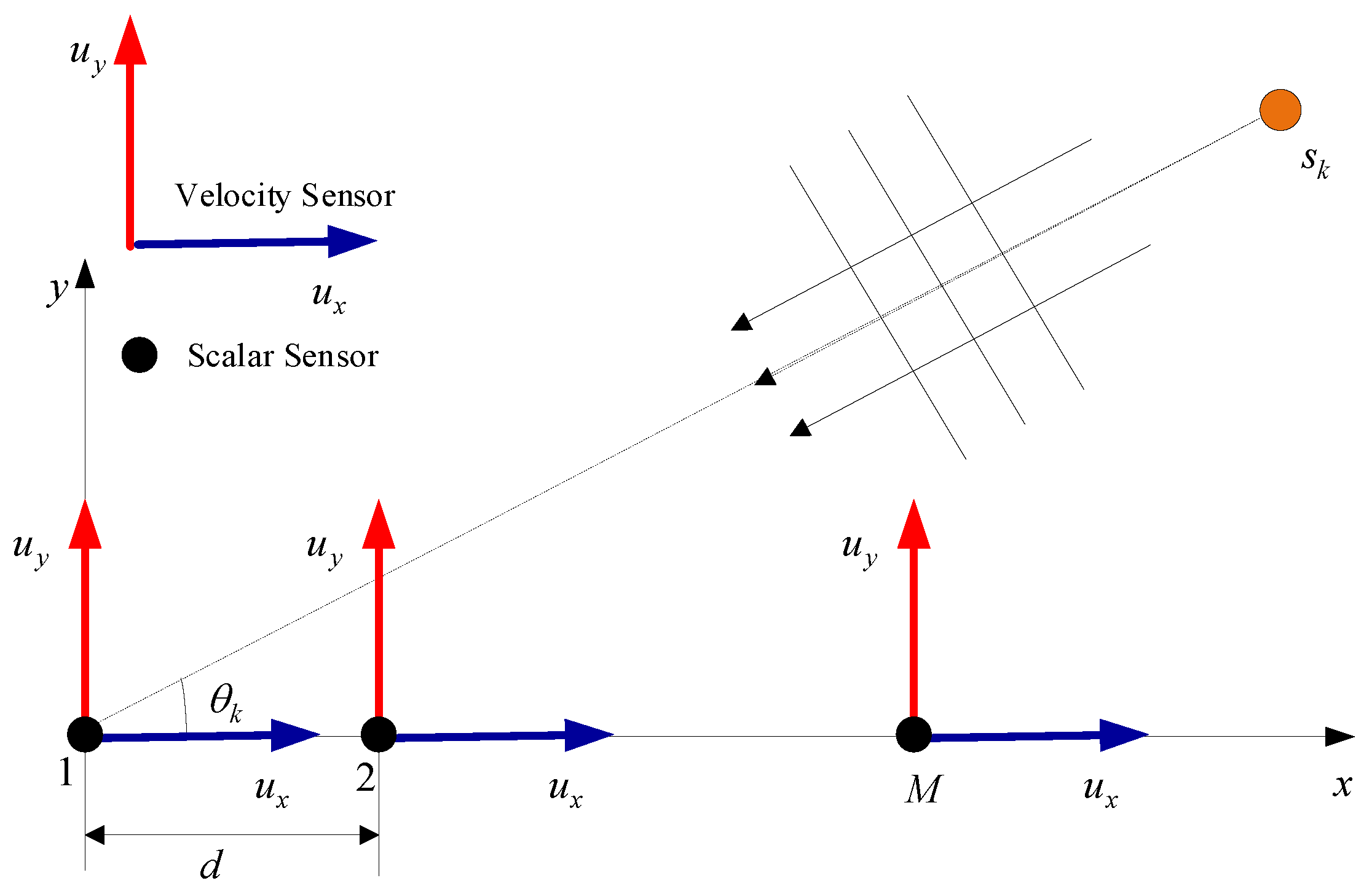
2.1. Data Model of AVSA

Assuming a uniform linear array consisting of M AVSs with the unit spacing between sensors d as depicted in Figure 1, K far-field equal power narrowband signals from different directions ${\theta }_k$$\left(k=1,2,\cdots ,K\right)$ are collected at the AVSA. The k-th signal object is incident on the m-th AVS, and its array manifold can be written as [11]

$$\mathbf{h}\left({\theta }_k\right)=\left[\begin{array}{c}1\\ cos{\theta }_k\\ sin{\theta }_k\end{array}\right].$$

(1)

Then, the array diverse matrix of AVSA can be represented as $\mathbf{A}\left(\mathsf{\theta }\right)=[\mathbf{a}\left({\theta }_1\right),\mathbf{a}\left({\theta }_1\right),$$\cdots ,\mathbf{a}\left({\theta }_K\right)]$, where $\mathbf{a}\left({\theta }_k\right)=\mathbf{q}\left({\theta }_k\right)\otimes \mathbf{h}\left({\theta }_k\right)$, $\mathbf{q}\left({\theta }_k\right)={\left[1,e^{-j2\pi dcos{\theta }_k/\lambda },\cdots ,e^{-j2\pi \left(M-1\right)dcos{\theta }_k/\lambda }\right]}^T$ is the acoustic pressure response parameter of the AVSA, and $\lambda$ is representing signal period. Then at time t, the output vector by the AVSA can be written as

$$\mathbf{x}\left(t\right)=\sum _{k=1}^K\mathbf{a}\left({\theta }_k\right)s_k\left(t\right)+\mathbf{w}\left(t\right)=\mathbf{A}\left(\mathsf{\theta }\right)\mathbf{s}\left(t\right)+\mathbf{w}\left(t\right),t=1,2,\cdots ,L,$$

(2)

and $\mathbf{x}\left(t\right)={\left[x_1\left(t\right),x_2\left(t\right),\cdots ,x_{3M}\left(t\right)\right]}^T$ is the output vector of AVSA at time t, $\mathbf{s}\left(t\right)={\left[s_1\left(t\right),s_2\left(t\right),\cdots ,s_K\left(t\right)\right]}^T$ is the waveform vector of the signal sources, $\mathbf{w}\left(t\right)=[w_1\left(t\right),w_2\left(t\right),$$\cdots ,w_{3M}\left(t\right){]}^T$ is the impulsive noise data gained by the AVSA, and L is representing the snapshot.

For ease of calculation, the concept of the sparse grid is introduced into the model. The angle space $-{180}^{\circ }\sim {180}^{\circ }$ is divided into N identical discrete nets, i.e., $\tilde{\mathsf{\theta }}=\left\{{\tilde{\theta }}_1,{\tilde{\theta }}_2,\cdots ,{\tilde{\theta }}_N\right\}$ and $N\gg K$, assuming that the DOAs of signal sources are placed at the discrete grids, i.e., ${\theta }_k\in \tilde{\mathsf{\theta }}$. At time t the sparse signal vector of the AVSA can be calculated as

$$\begin{array}{c}\hfill \mathbf{x}\left(t\right)=\sum _{n=1}^N\mathbf{a}\left({\tilde{\theta }}_n\right){\tilde{\mathbf{s}}}_n\left(t\right)+\mathbf{w}\left(t\right)=\mathbf{A}\left(\tilde{\mathsf{\theta }}\right)\tilde{\mathbf{s}}\left(t\right)+\mathbf{w}\left(t\right),\end{array}$$

(3)

and likewise $\mathbf{A}\left(\tilde{\mathsf{\theta }}\right)=\left[\mathbf{a}\left({\tilde{\theta }}_1\right),\mathbf{a}\left({\tilde{\theta }}_2\right),\cdots ,\mathbf{a}\left({\tilde{\theta }}_N\right)\right]$ is the array manifold matrix of $3M\times N$, and $\tilde{\mathbf{s}}\left(t\right)={\left[{\tilde{s}}_1\left(t\right),{\tilde{s}}_2\left(t\right),\cdots ,{\tilde{s}}_N\left(t\right)\right]}^T$ is the waveform vector of the signal with dimensions $N\times 1$.

2.2. $\alpha$-Stable Distribution Model

The $\alpha$-stable distribution is utilized as the noise model since it is famous for its heavy tail, stability and non-Gaussian characteristics, which enable it to perfectly simulate extreme anomalies in the signal. Unfortunately, there is no PDF closed-form expression for $\alpha$-stable spreading. Thus, its fitness criterion is often utilized to express noise as [45]

$$\varphi \left(t\right)=e^{\left\{j\mu t-\gamma {\left|t\right|}^{\alpha }\left[1+j\beta \mathrm{sgn}\left(t\right)\varpi \left(t,\alpha \right)\right]\right\}}$$

(4)

with

$$\mathrm{sgn}\left(t\right)=\{\begin{array}{c}1\\ 0\\ -1\end{array}\begin{array}{c}t>0\\ t=0\\ t<0\end{array}$$

(5)

and

$$\varpi \left(t,\alpha \right)=\{\begin{array}{c}tan\left({\displaystyle \frac{\alpha \pi }{2}}\right)\left(\alpha \ne 1\right)\\ {\displaystyle \frac{2}{\pi }}log\left|t\right|\left(\alpha =1\right)\end{array},$$

(6)

and $\alpha$$\left(0<\alpha \le 2\right)$ is the characteristic exponent, that manages the thickness of the tail of the PDF, $\gamma$$\left(\gamma >0\right)$ is the diffusion variable, which is identical to the variance of Gaussian distribution, $\mu$ denotes the position parameter, and $\beta$$\left(-1\le \beta \le 1\right)$ is the proportionality parameter. Noting that the $\alpha$-stable spreading is proportional about $\mu$, thus, it is named symmetric $\alpha$-stable ($\mathrm{S}\alpha \mathrm{S}$) spreading when $\beta =0$. The $\mathrm{S}\alpha \mathrm{S}$ spreading represents a different PDF after different parameters are selected. Therefore, it is equivalent to the Gaussian distribution when $\alpha =2$ and $\beta =0$, and it denotes the Cauchy distribution when $\alpha =1$ and $\beta =0$.

3. The Proposed IWPN-SIA Algorithm

In this section, the IWPN-SIA algorithm is projected to realize the efficient estimation of DOA via the AVSA in the presence of impulsive noise. Firstly, by utilizing an infinite norm weighting technique, the impact of high outliers is mitigated through extensive numerical scaling. Subsequently, the Frobenius norm is extended to lower orders, and then a new cost function based on p-order is formulated to obtain the DOA estimation. Simultaneously, eigenvalue decomposition is incorporated to further attenuate noise.

3.1. Weighted Preconditioning with the Infinite Norm

To mitigate the impact of outliers and obtain a bounded covariance matrix, the weighted term is defined as

$$\mathsf{\ell }\left(t\right)=\frac{1}{{∥{\mathbf{x}}_m\left(t\right)∥}_{\infty }},m=1,2\cdots ,3M,$$

(7)

where ${∥{\mathbf{x}}_m\left(t\right)∥}_{\infty }$ denotes infinite norm of the signal vector $\mathbf{x}\left(t\right)\in 3M\times 1$. The weighted signal vector of the AVSA at time t is rewritten as

$$\begin{array}{cc}\hfill \mathbf{y}\left(t\right)& =\mathbf{x}\left(t\right)\mathsf{\ell }\left(t\right)\hfill \\ \hfill & =\mathbf{A}\left(\tilde{\mathsf{\theta }}\right)\tilde{\mathbf{s}}\left(t\right)\mathsf{\ell }\left(t\right)+\mathbf{w}\left(t\right)\mathsf{\ell }\left(t\right)\hfill \\ \hfill & =\mathbf{A}\left(\tilde{\mathsf{\theta }}\right){\tilde{\mathbf{s}}}_w\left(t\right)+\mathbf{v}\left(t\right),\hfill \end{array}$$

(8)

so $\mathbf{y}\left(t\right)={\left[y_1\left(t\right),y_2\left(t\right),\cdots ,y_{3M}\left(t\right)\right]}^T$ is the weighted array signal output vector, ${\tilde{\mathbf{s}}}_w\left(t\right)=\tilde{\mathbf{s}}\left(t\right)\mathsf{\ell }\left(t\right)={\left[{\tilde{s}}_{w1}\left(t\right),{\tilde{s}}_{w2}\left(t\right),\cdots ,{\tilde{s}}_{wN}\left(t\right)\right]}^T$ is the weighted waveform vector, and $\mathbf{v}\left(t\right)=\mathbf{w}\left(t\right)\mathsf{\ell }\left(t\right)$$={[v_1\left(t\right),v_2\left(t\right),\cdots ,v_{3M}\left(t\right)]}^T$ is the noise weighted vector.

It can be seen from (7) and (8) that the weighted processing technique is blind since it does not necessitate any previous information of impulsive noise data. Hence, it is also adaptable for use with various impulsive noise designs. In addition, the higher the outlier in the observed data, the greater the inhibition of these outliers in the weighted processing, demonstrating the dominance of this approach in processing high outliers.

Built on (8), the weighted correlation information of the AVSA is obtained as

$$\mathbf{R}=E\left\{\mathbf{Y}{\mathbf{Y}}^H\right\}=\mathbf{A}\left(\tilde{\mathsf{\theta }}\right){\mathsf{\Sigma }}_s{\mathbf{A}}^H\left(\tilde{\mathsf{\theta }}\right)+{\eta }_v^2\mathbf{I},$$

(9)

as with $\mathbf{Y}=\left[\mathbf{y}\left(1\right),\mathbf{y}\left(2\right),\cdots ,\mathbf{y}\left(L\right)\right]$, ${\mathsf{\Sigma }}_s=E\left\{{\tilde{\mathbf{s}}}_w\left(t\right){\tilde{\mathbf{s}}}_w^H\left(t\right)\right\}=\mathcal{D}\left\{{\eta }_1^2,{\eta }_2^2,\cdots ,{\eta }_N^2\right\}$ with ${\eta }_n^2=E\left\{|{\tilde{s}}_{wn}\left(t\right){|}^2\right\}$ denoting the power of the n-th weighted signal, and ${\eta }_v^2$ is the weighted noise strength of the respective observer. As mentioned in [36,46], the weighted array noises from separate observers exhibit no correlation, the weighted array signals from different sensors also show no correlation, and there is no correlation between the weighted array noises and signals. Consequently, the eigenvalue division of matrix $\mathbf{R}$ is subsequently performed by

$$\begin{array}{cc}\hfill \mathbf{R}& =\sum _{m=1}^K{\lambda }_m{a}_m{a}_m^H+\sum _{m=K+1}^{3M}{\lambda }_m{a}_m{a}_m^H\hfill \\ \hfill & ={\mathbf{U}}_s{\mathsf{\Lambda }}_s{\mathbf{U}}_s^H+{\mathbf{U}}_v{\mathsf{\Lambda }}_v{\mathbf{U}}_v^H={\mathbf{R}}_s+{\mathbf{R}}_v,\hfill \end{array}$$

(10)

where ${\lambda }_1,\cdots ,{\lambda }_K,{\lambda }_{K+1},\cdots ,{\lambda }_{3M}$ are the $3M$ eigenvalues of the matrix $\mathbf{R}$, $a_1,\cdots a_K,a_{K+1},$$\cdots ,a_{3M}$ are the corresponding eigenvectors, ${\mathsf{\Lambda }}_s$ denotes a diagonal matrix consisting of K large eigenvalues, ${\mathbf{U}}_s$ signifies the signal segment formed from eigenvectors corresponding to the large eigenvalues, ${\mathsf{\Lambda }}_v$ represents the diagonal matrix of $3M-K$ small eigenvalues, ${\mathbf{U}}_v$ expresses are called the noise subspace, which is also formed from the eigenvectors corresponding to the small eigenvalues, signal correlation matrix is denoted with ${\mathbf{R}}_s$, and ${\mathbf{R}}_v$ stands for the noise correlation matrix. In practical applications, the estimated weighted array covariance matrix $\mathbf{R}$ usually needs to be swapped by the prototype correlation matrix $\widehat{\mathbf{R}}={\displaystyle \frac{1}{L}}{\sum }_{t=1}^L\mathbf{y}\left(t\right){\mathbf{y}}^H\left(t\right)$.

3.2. A Sparse Iterative Algorithm Based on p-Norm

Based on the concept of FLOS [33], the low-order covariance matrix is defined as

$${\mathbf{R}}_c=E\left\{\mathbf{Y}{\mathbf{Y}}^H\mathbf{Z}\right\},$$

(11)

where $\mathbf{Z}=\mathcal{D}\left\{{\left|y_1\left(t\right)\right|}^{p-2},{\left|y_2\left(t\right)\right|}^{p-2},\cdots ,{\left|y_{3M}\left(t\right)\right|}^{p-2}\right\}$ is the low-order weighted matrix. It is obvious that the diagonal element of the low-order covariance ${\mathbf{R}}_c$ represents the signal power, and its value is closely related to p. Thus, ${\mathbf{R}}_c$ can be rewritten as

$${\mathbf{R}}_c=\mathbf{A}\left(\tilde{\mathsf{\theta }}\right)\mathbf{Q}{\mathbf{A}}^H\left(\tilde{\mathsf{\theta }}\right),$$

(12)

where $\mathbf{Q}=\mathcal{D}\left\{{\tilde{q}}_1,{\tilde{q}}_2,\cdots ,{\tilde{q}}_N\right\}$ with ${\tilde{q}}_n={\displaystyle \frac{1}{L}}\sum _{t=1}^L{\left|{\tilde{s}}_{wn}\left(t\right)\right|}^p$. Based on (8), the signal correlation matrix from the n-th grid is given as

$$\begin{array}{c}\hfill {\mathbf{R}}_n={\mathbf{A}}_n{\mathbf{A}}_n^H\frac{1}{L}\sum _{t=1}^L{\left|{\tilde{s}}_{wn}\left(t\right)\right|}^p={\tilde{q}}_n{\mathbf{A}}_n{\mathbf{A}}_n^H,\end{array}$$

(13)

where the n-th column input of $\mathbf{A}\left(\tilde{\mathsf{\theta }}\right)$ is represented with ${\mathbf{A}}_n$. Next, the correlation matrix of interference combined with noise on the n-th grid can be represented as

$$\begin{array}{c}\hfill {\mathsf{\Theta }}_n={\mathbf{R}}_c-{\mathbf{R}}_n={\mathbf{R}}_c-{\tilde{q}}_n{\mathbf{A}}_n{\mathbf{A}}_n^H.\end{array}$$

(14)

Based on [22,47], we can obtain the inverse of the matrix ${\mathsf{\Theta }}_n$

$$\begin{array}{c}\hfill {\mathsf{\Theta }}_n^{-1}={{\mathbf{R}}_c}^{-1}+{\tilde{q}}_n\frac{{{\mathbf{R}}_c}^{-1}{\mathbf{A}}_n{\mathbf{A}}_n^H{{\mathbf{R}}_c}^{-1}}{1-{\tilde{q}}_n{\mathbf{A}}_n^H{{\mathbf{R}}_c}^{-1}{\mathbf{A}}_n}.\end{array}$$

(15)

To further enhance the suppression ability of outlier, the Frobenius norm-based method in [22] is extended to p-norm. The cost function is constructed as follows

$$\begin{array}{c}\hfill g\left({\tilde{q}}_n\right)={∥{\mathsf{\Theta }}_n^{-1}\left({\mathbf{R}}_s-{\tilde{q}}_n{\mathbf{A}}_n{\mathbf{A}}_n^H\right)∥}_p^p.\end{array}$$

(16)

Based on the statement in [48] and the operational relationship between the matrix norm and the trace in [47], for any matrix $\mathbf{B}\in M\times M$, it holds that

$$\begin{array}{c}\hfill {∥\mathbf{B}∥}_p^p={(tr{\{{\mathbf{B}}^p\}}^{\frac{1}{p}})}^p=tr\left\{{\mathbf{B}}^p\right\}.\end{array}$$

(17)

        According to (17), (16) can be further transformed into

$$\begin{array}{cc}\hfill g\left({\tilde{q}}_n\right)& ={∥{\mathsf{\Theta }}_n^{-1}({\mathbf{R}}_s-{\tilde{q}}_n{\mathbf{A}}_n{\mathbf{A}}_n^H)∥}_p^p\hfill \\ \hfill & =tr\{\sum _{\zeta =1}^{3M}\sum _{\eta =1}^{3M}{\left[{\mathsf{\Theta }}_n^{-1}({\mathbf{R}}_s-{\tilde{q}}_n{\mathbf{A}}_n{\mathbf{A}}_n^H)\right]}_{\zeta }\hfill \\ \hfill & \times abs{\left\{{\left[{\mathsf{\Theta }}_n^{-1}({\mathbf{R}}_s-{\tilde{q}}_n{\mathbf{A}}_n{\mathbf{A}}_n^H)\right]}_{\eta }\right\}}^{p-2}{{\left[{\mathsf{\Theta }}_n^{-1}({\mathbf{R}}_s-{\tilde{q}}_n{\mathbf{A}}_n{\mathbf{A}}_n^H)\right]}_{\eta }}^{*}\}\hfill \\ \hfill & =tr\{{\mathsf{\Theta }}_n^{-1}({\mathbf{R}}_s-{\tilde{q}}_n{\mathbf{A}}_n{\mathbf{A}}_n^H)abs{\left\{{\mathsf{\Theta }}_n^{-1}({\mathbf{R}}_s-{\tilde{q}}_n{\mathbf{A}}_n{\mathbf{A}}_n^H)\right\}}^{p-2}\hfill \\ \hfill & \times {({\mathbf{R}}_s-{\tilde{q}}_n{\mathbf{A}}_n{\mathbf{A}}_n^H)}^H{\mathsf{\Theta }}_n^{-1}\}\hfill \\ \hfill & =tr\left\{({\mathbf{R}}_s-{\tilde{q}}_n{\mathbf{A}}_n{\mathbf{A}}_n^H){\mathsf{\Theta }}_n^{-2}{\mathsf{\Psi }}^2{({\mathbf{R}}_s-{\tilde{q}}_n{\mathbf{A}}_n{\mathbf{A}}_n^H)}^H\right\},\hfill \end{array}$$

(18)

where $\mathsf{\Psi }$ is a low-order weighted matrix, which is defined as

$$\begin{array}{cc}\hfill \mathsf{\Psi }& =\left[\begin{array}{cccc}{\left|{\mathsf{\Gamma }}_{11}\right|}^{\frac{p-2}{2}}& {\left|{\mathsf{\Gamma }}_{12}\right|}^{\frac{p-2}{2}}& \cdots & {\left|{\mathsf{\Gamma }}_{1\eta }\right|}^{\frac{p-2}{2}}\\ {\left|{\mathsf{\Gamma }}_{21}\right|}^{\frac{p-2}{2}}& {\left|{\mathsf{\Gamma }}_{22}\right|}^{\frac{p-2}{2}}& \cdots & {\left|{\mathsf{\Gamma }}_{2\eta }\right|}^{\frac{p-2}{2}}\\ ⋮& ⋮& \ddots & ⋮\\ {\left|{\mathsf{\Gamma }}_{\eta 1}\right|}^{\frac{p-2}{2}}& {\left|{\mathsf{\Gamma }}_{\eta 2}\right|}^{\frac{p-2}{2}}& \cdots & {\left|{\mathsf{\Gamma }}_{\eta \eta }\right|}^{\frac{p-2}{2}}\end{array}\right]\hfill \end{array}$$

(19)

with $\mathsf{\Gamma }={\mathsf{\Theta }}_n^{-1}({\mathbf{R}}_s-{\tilde{q}}_n{\mathbf{A}}_n{\mathbf{A}}_n^H)$, $\eta =3M$, and ${\mathsf{\Gamma }}_{\zeta \eta }$ denoting the entity in $\eta$-th column and $\zeta$-th row of $\mathsf{\Gamma }$. To simplify the calculation, its diagonal elements are extracted to create a new weighted matrix $\mathbf{\Xi }$, which is defined as

$$\begin{array}{c}\hfill \mathbf{\Xi }=\left[\begin{array}{cccc}{\left|{\mathsf{\Gamma }}_{11}\right|}^{\frac{p-2}{2}}& 0& \cdots & 0\\ 0& {\left|{\mathsf{\Gamma }}_{22}\right|}^{\frac{p-2}{2}}& \cdots & 0\\ ⋮& ⋮& \ddots & ⋮\\ 0& 0& \cdots & {\left|{\mathsf{\Gamma }}_{\eta \eta }\right|}^{\frac{p-2}{2}}\end{array}\right].\end{array}$$

(20)

Then, (18) can be further simplified as

$$\begin{array}{cc}\hfill g\left({\tilde{q}}_n\right)& ={∥{\mathsf{\Theta }}_n^{-1}\left({\mathbf{R}}_s-{\tilde{q}}_n{\mathbf{A}}_n{\mathbf{A}}_n^H\right)∥}_p^p\hfill \\ \hfill & =tr\left\{\left({\mathbf{R}}_s-{\tilde{q}}_n{\mathbf{A}}_n{\mathbf{A}}_n^H\right){\mathsf{\Theta }}_n^{-2}{\mathbf{\Xi }}^2{\left({\mathbf{R}}_s-{\tilde{q}}_n{\mathbf{A}}_n{\mathbf{A}}_n^H\right)}^H\right\}\hfill \\ \hfill & =tr\left\{{\mathbf{R}}_s{\mathsf{\Theta }}_n^{-2}{\mathbf{\Xi }}^2{\mathbf{R}}_s^H\right\}+tr\left\{{\left({\tilde{q}}_n{\mathbf{A}}_n^H{\mathsf{\Theta }}_n^{-1}\mathbf{\Xi }{\mathbf{A}}_n\right)}^2\right\}\hfill \\ \hfill & -2tr\left\{{\tilde{q}}_n{\mathbf{A}}_n^H{\mathsf{\Theta }}_n^{-1}\mathbf{\Xi }{\mathbf{R}}_s\mathbf{\Xi }{\mathsf{\Theta }}_n^{-1}{\mathbf{A}}_n\right\}\hfill \\ \hfill & =tr\left\{{\mathbf{R}}_s{\mathsf{\Theta }}_n^{-2}{\mathbf{\Xi }}^2{\mathbf{R}}_s^H\right\}+{\left({\tilde{q}}_n{\mathbf{A}}_n^H{\mathsf{\Theta }}_n^{-1}\mathbf{\Xi }{\mathbf{A}}_n\right)}^2\hfill \\ \hfill & -2{\tilde{q}}_n{\mathbf{A}}_n^H{\mathsf{\Theta }}_n^{-1}\mathbf{\Xi }{\mathbf{R}}_s\mathbf{\Xi }{\mathsf{\Theta }}_n^{-1}{\mathbf{A}}_n.\hfill \end{array}$$

(21)

The initial and secondary derivatives of $g\left({\tilde{q}}_n\right)$ in terms of ${\tilde{q}}_n$ are

$$\begin{array}{cc}\hfill g^{\prime }\left({\tilde{q}}_n\right)& =2{\tilde{q}}_n{\left({\mathbf{A}}_n^H{\mathsf{\Theta }}_n^{-1}\mathbf{\Xi }{\mathbf{A}}_n\right)}^2-2{\mathbf{A}}_n^H{\mathsf{\Theta }}_n^{-1}\mathbf{\Xi }{\mathbf{R}}_s\mathbf{\Xi }{\mathsf{\Theta }}_n^{-1}{\mathbf{A}}_n,\hfill \end{array}$$

(22)

and

$$\begin{array}{c}\hfill g^{″}\left({\tilde{q}}_n\right)=2{\left({\mathbf{A}}_n^H{\mathsf{\Theta }}_n^{-1}\mathbf{\Xi }{\mathbf{A}}_n\right)}^2.\end{array}$$

(23)

Based on (23), we can have $g^{″}\left({\tilde{q}}_n\right)>0$, showing that $g^{\prime }\left({\tilde{q}}_n\right)$ has a unique solution. Setting $g^{\prime }\left({\tilde{q}}_n\right)=0$, we obtain

$$\begin{array}{c}\hfill {\tilde{q}}_n=\frac{{\mathbf{A}}_n^H{\mathsf{\Theta }}_n^{-1}\mathbf{\Xi }{\mathbf{R}}_s\mathbf{\Xi }{\mathsf{\Theta }}_n^{-1}{\mathbf{A}}_n}{{\left({\mathbf{A}}_n^H{\mathsf{\Theta }}_n^{-1}\mathbf{\Xi }{\mathbf{A}}_n\right)}^2}.\end{array}$$

(24)

By substituting (15) into (24), the following can be obtained,

$$\begin{array}{cc}\hfill {\tilde{q}}_n& =\frac{{\mathbf{A}}_n^H\left({{\mathbf{R}}_c}^{-1}\left(1+{\tilde{q}}_n\xi \right)\right)\mathbf{\Xi }{\mathbf{R}}_s\mathbf{\Xi }\left({{\mathbf{R}}_c}^{-1}\left(1+{\tilde{q}}_n\xi \right)\right){\mathbf{A}}_n}{{\left({\mathbf{A}}_n^H\left({{\mathbf{R}}_c}^{-1}\left(1+{\tilde{q}}_n\xi \right)\right)\mathbf{\Xi }{\mathbf{A}}_n\right)}^2}\hfill \\ \hfill & =\frac{{\left(1+{\tilde{q}}_n\xi \right)}^2{\mathbf{A}}_n^H{{\mathbf{R}}_c}^{-1}\mathbf{\Xi }{\mathbf{R}}_s\mathbf{\Xi }{{\mathbf{R}}_c}^{-1}{\mathbf{A}}_n}{{\left(1+{\tilde{q}}_n\xi \right)}^2{\left({\mathbf{A}}_n^H{{\mathbf{R}}_c}^{-1}\mathbf{\Xi }{\mathbf{A}}_n\right)}^2}\hfill \\ \hfill & =\frac{{\mathbf{A}}_n^H{{\mathbf{R}}_c}^{-1}\mathbf{\Xi }{\mathbf{R}}_s\mathbf{\Xi }{{\mathbf{R}}_c}^{-1}{\mathbf{A}}_n}{{\left({\mathbf{A}}_n^H{{\mathbf{R}}_c}^{-1}\mathbf{\Xi }{\mathbf{A}}_n\right)}^2},\hfill \end{array}$$

(25)

where $\xi ={\displaystyle \frac{{\mathbf{A}}_n^H{{\mathbf{R}}_c}^{-1}{\mathbf{A}}_n}{1-{\tilde{q}}_n{\mathbf{A}}_n^H{{\mathbf{R}}_c}^{-1}{\mathbf{A}}_n}}$. It is obvious that estimating ${\tilde{q}}_n$ by (25) requires the prior information of $\mathbf{\Xi }$, and then solving $\mathbf{\Xi }$ also requires the prior information of ${\tilde{q}}_n$. Therefore, an iterative algorithm must be used to estimate ${\tilde{q}}_n$. Assuming ${\widehat{q}}_n^{\left(j+1\right)}$ is the estimation of ${\tilde{q}}_n$ in the $(j+1)$-th time. Next, ${\widehat{q}}_n^{\left(j+1\right)}$ is obtained as

$$\begin{array}{c}\hfill {\widehat{q}}_n^{\left(j+1\right)}=\frac{{\mathbf{A}}_n^H{{\mathbf{R}}_c}^{-1\left(j\right)}{\mathbf{\Xi }}^{\left(j\right)}{\mathbf{R}}_s{\mathbf{\Xi }}^{\left(j\right)}{{\mathbf{R}}_c}^{-1\left(j\right)}{\mathbf{A}}_n}{{\left({\mathbf{A}}_n^H{{\mathbf{R}}_c}^{-1\left(j\right)}{\mathbf{\Xi }}^{\left(j\right)}{\mathbf{A}}_n\right)}^2},\end{array}$$

(26)

where

$$\begin{array}{c}\hfill {\mathbf{\Xi }}^{\left(j\right)}=\mathcal{D}\left\{\right|{{\mathsf{\Gamma }}_{11}}^{\left(j\right)}{|}^{\frac{p-2}{2}},|{{\mathsf{\Gamma }}_{22}}^{\left(j\right)}{|}^{\frac{p-2}{2}},\cdots ,\left|{{\mathsf{\Gamma }}_{\eta \eta }}^{\left(j\right)}{|}^{\frac{p-2}{2}}\right\}\end{array}$$

(27)

with

$$\begin{array}{cc}\hfill {\mathsf{\Gamma }}^{\left(j\right)}& ={\left({\mathsf{\Theta }}_n^{\left(j\right)}\right)}^{-1}({\mathbf{R}}_s-{\widehat{q}}_n^{\left(j\right)}{\mathbf{A}}_n{\mathbf{A}}_n^H)\hfill \\ \hfill & ={({{\mathbf{R}}_c}^{\left(j\right)}-{\widehat{q}}_n^{\left(j\right)}{\mathbf{A}}_n{\mathbf{A}}_n^H)}^{-1}({\mathbf{R}}_s-{\widehat{q}}_n^{\left(j\right)}{\mathbf{A}}_n{\mathbf{A}}_n^H)\hfill \end{array}$$

(28)

and

$$\begin{array}{c}\hfill {{\mathbf{R}}_c}^{\left(j\right)}=\mathbf{A}\left(\tilde{\mathsf{\theta }}\right){\widehat{\mathbf{Q}}}^{\left(j\right)}\mathbf{A}\left(\tilde{\mathsf{\theta }}\right)\end{array}$$

(29)

with

$$\begin{array}{c}\hfill {\widehat{\mathbf{Q}}}^{\left(j\right)}=\mathcal{D}\left\{{\widehat{q}}_1^{\left(j\right)},{\widehat{q}}_2^{\left(j\right)},\cdots ,{\widehat{q}}_N^{\left(j\right)}\right\}.\end{array}$$

(30)

Ultimately, the presented method is consolidated as Algorithm 1.   

Algorithm 1: Infinite Weighted p-norm Sparse Iterative Algorithm

1: Calculate the weighting term $\mathsf{\ell }\left(t\right)$ and the weighted signal vector $\mathbf{y}\left(t\right)$ with (7) and (8), respectively. 2: Obtain the low-order sample covariance matrix ${\mathbf{R}}_c$ with (11). 3: Perform the eigenvalue decomposition to obtain the signal covariance matrix ${\mathbf{R}}_s$ with (10). 4: Initialize ${\mathbf{Q}}^{\left(0\right)}=\mathcal{D}\left\{{\tilde{q}}_1^{\left(0\right)},{\tilde{q}}_2^{\left(0\right)},\cdots ,{\tilde{q}}_N^{\left(0\right)}\right\}$ with ${\tilde{q}}_n^{\left(0\right)}={\mathbf{A}}_n^H{\mathbf{R}}_s{\mathbf{A}}_n$. 5: Update ${{\mathbf{R}}_c}^{\left(j\right)}$ with (29). 6: Calculate the low-order weight matrix ${\mathbf{\Xi }}^{\left(j\right)}$ by (27). 7: Update ${\widehat{q}}_n^{(j+1)}$ with (26) with $n=1,2,\cdots ,N$. 8: Update ${\widehat{\mathbf{Q}}}^{\left(j+1\right)}=\mathcal{D}\left\{{\widehat{q}}_1^{\left(j+1\right)},{\widehat{q}}_2^{\left(j+1\right)},\cdots ,{\widehat{q}}_N^{\left(j+1\right)}\right\}$. 9: Repeat steps 5–8 until $\parallel {\widehat{\mathbf{Q}}}^{\left(j+1\right)}-{\widehat{\mathbf{Q}}}^{\left(j\right)}{\parallel }_2^2\le \upsilon$ or $j\ge T_{max}$, where $\upsilon$ is the error tolerance. 10: Output the DOA by performing a spectral peak search on ${\widehat{\mathbf{q}}}^{(j+1)}=\left[{\widehat{q}}_1^{\left(j+1\right)},{\widehat{q}}_2^{\left(j+1\right)},\cdots ,{\widehat{q}}_N^{\left(j+1\right)}\right]$.

4. Simulation Results and Discussions

Here, we compare the designed IWPN-SIA paradigm with classical algorithms MUSIC [12], IAA [22], and advanced algorithms for impulsive noise including FLOM-MUSIC [34] and WARD-MUSIC [36]. Unless otherwise stated, a ULA with $M=5$ AVSs are used in the following simulations, the scanning range $-{180}^{\circ }\sim {180}^{\circ }$ is divided into 361 grids with a $1^{\circ }$ interval, the error tolerance $\upsilon$ is set to ${10}^{-3}$, and the maximum iteration times $T_{max}$ is 25. The impulsive noise is modeled as $\mathrm{S}\alpha \mathrm{S}$ distribution, i.e., $\beta =0$, and the diffusion variable $\gamma$ is fixed to 1. Due to the features of $\alpha$-stable distribution, the commonly used SNR becomes meaningless. To quantify the signal power and noise diffusion ratio, the generalized signal–to–noise ratio (GSNR) is computed with [27] as

$$\begin{array}{c}\hfill \mathrm{GSNR}=\frac{\mathrm{E}\{{\left|\mathbf{s}\left(t\right)\right|}^2\}}{{\gamma }^{\alpha }}.\end{array}$$

(31)

The two incoming waves of DOAs are ${\theta }_1={60}^{\circ }$, ${\theta }_2={134}^{\circ }$, respectively. For each simulation, 2000 Monte Carlo trials ($N_m=2000$) are executed. The resolution likelihood and root mean square error (RMSE) are examined for these algorithms. Among them, it is believed that the DOA prediction of two objects can be successfully distinguished whether the DOA estimation errors of these objects are lower than $\tau =2^{\circ }$. Suppose that the number of successful resolutions is $N_c$ in $N_m$ Monte Carlo trials, then the resolution probability is shown as $N_c/N_m$. The RMSE is defined as

$$\begin{array}{c}\hfill \mathrm{RMSE}=\frac{1}{N_m}\sum _{i=1}^{N_m}\sqrt{\frac{1}{K}{\sum _{k=1}^K\left({\widehat{\theta }}_{k,i}-{\theta }_k\right)}^2},\end{array}$$

(32)

in the i-th Monte Carlo trial, and ${\widehat{\theta }}_{k,i}$ is the k-th signal estimated DOA.

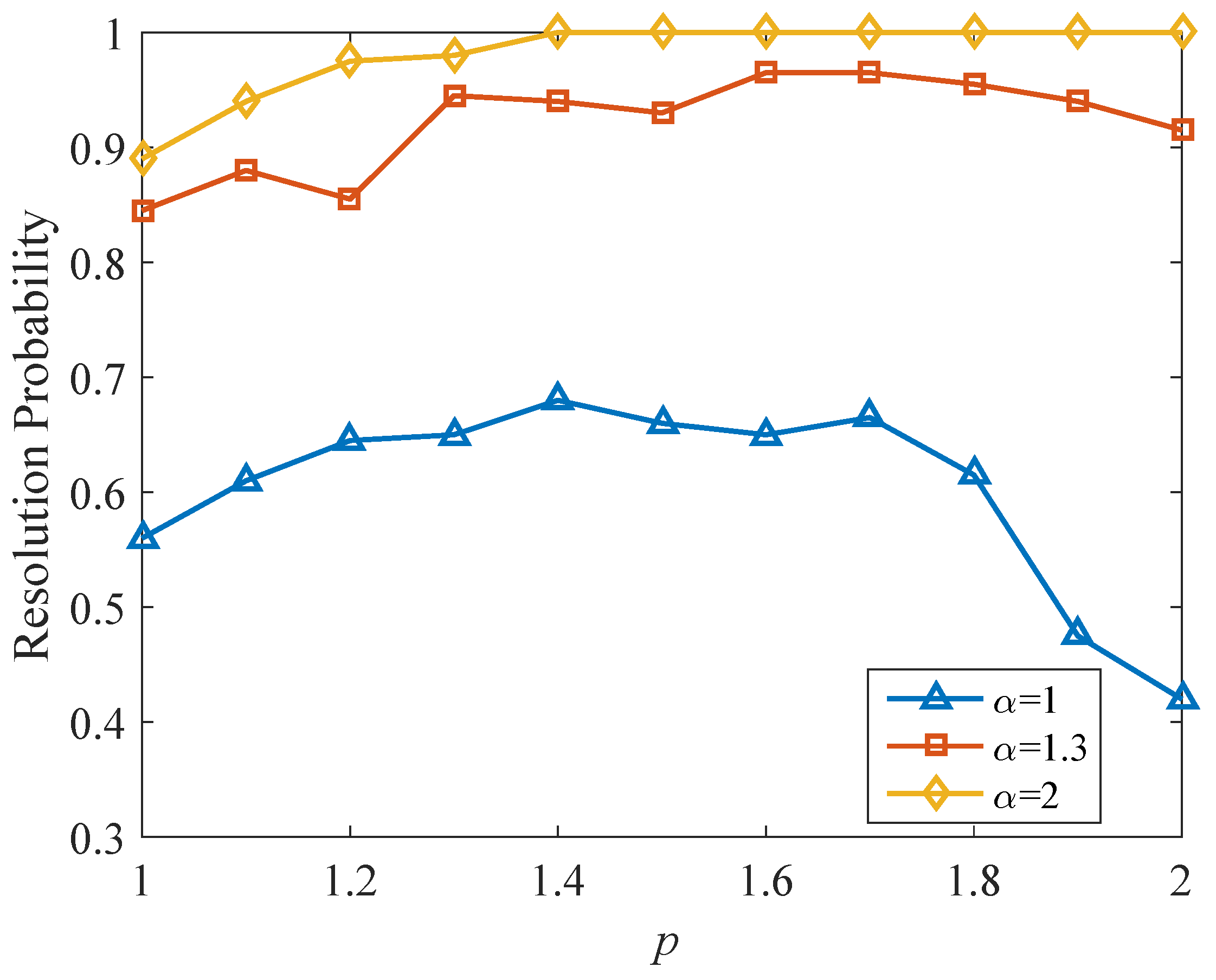
4.1. The Influence of p on Resolution Probability and RMSE

Here, we provide the relationship between p and resolution probability and RMSE to determine the value of p.

The simulation results are depicted in Figure 2 and Figure 3, respectively, with GSNR = −2 dB and $L=$ 300 where we consider three cases: $\alpha =1$, $\alpha =1.3$, and $\alpha =2$. It can be seen from Figure 2 that the resolution probability of the IWPN-SIA method can reach 100% when $\alpha =2$ and $p>1.4$. Although the resolution probability of the IWPN-SIA method cannot reach 100% within the range of 1 to 2 for p when $\alpha =1.3$, it has the highest resolution probability when p is approximately 1.7. It is obvious that compared to $\alpha =1.3$ and $\alpha =2$, the resolution probability of the IWPN-SIA method is the worst when $\alpha =1$, but it can be seen that its resolution probability is relatively high when p is in the range of 1.4 to 1.7. In addition, it can be seen in Figure 3 that the RMSE of the IWPN-SIA method tends to stabilize when $\alpha =2$ and $p>1.3$. Obviously, its RMSE is the smallest when $\alpha =1.3$ and p is around 1.8. Moreover, it can be seen that the RMSE is relatively large throughout the entire range of p when $\alpha =1$, but its RMSE is the smallest when $p=1.7$. Therefore, in the following simulation experiments, p is fixed to 1.7.

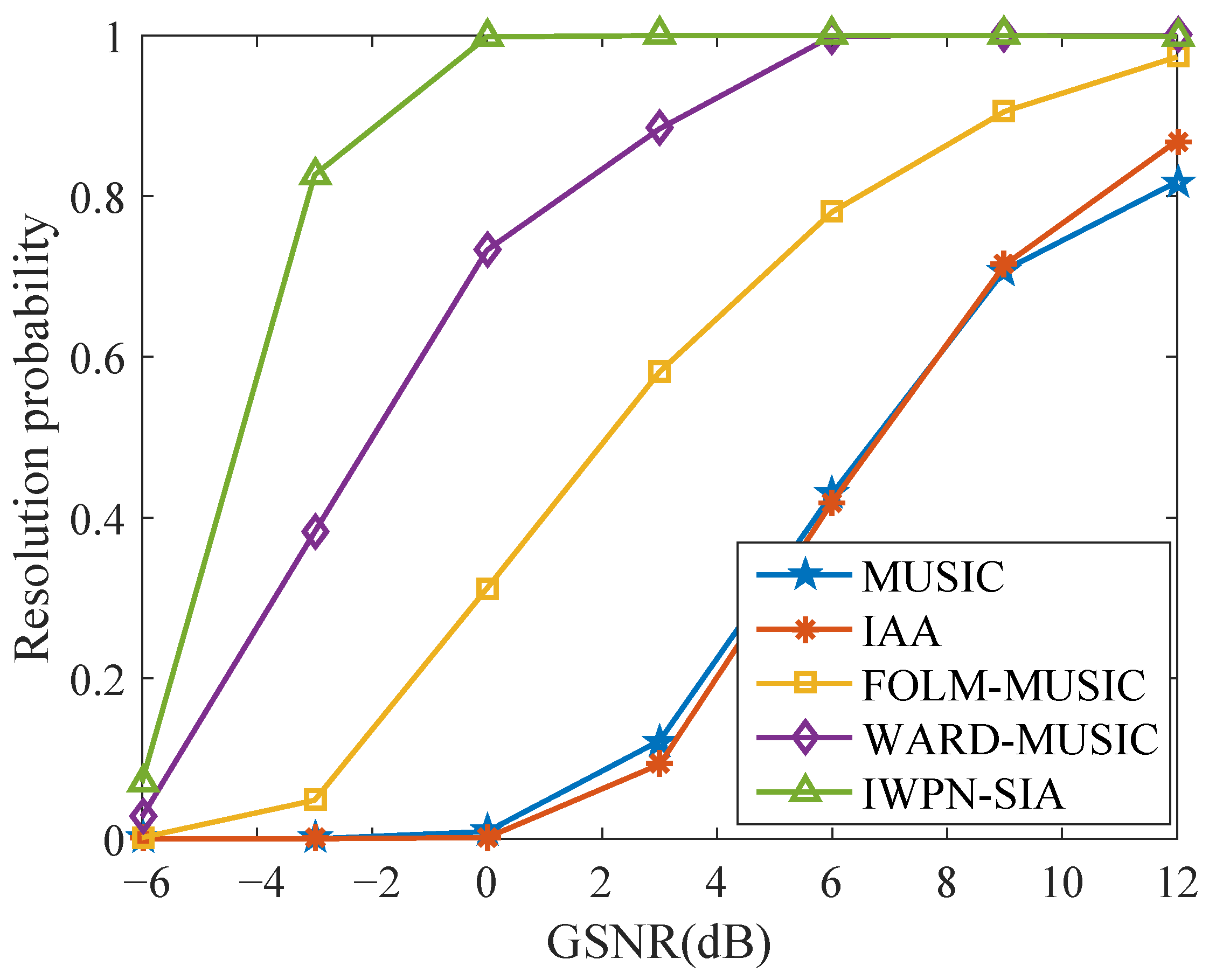
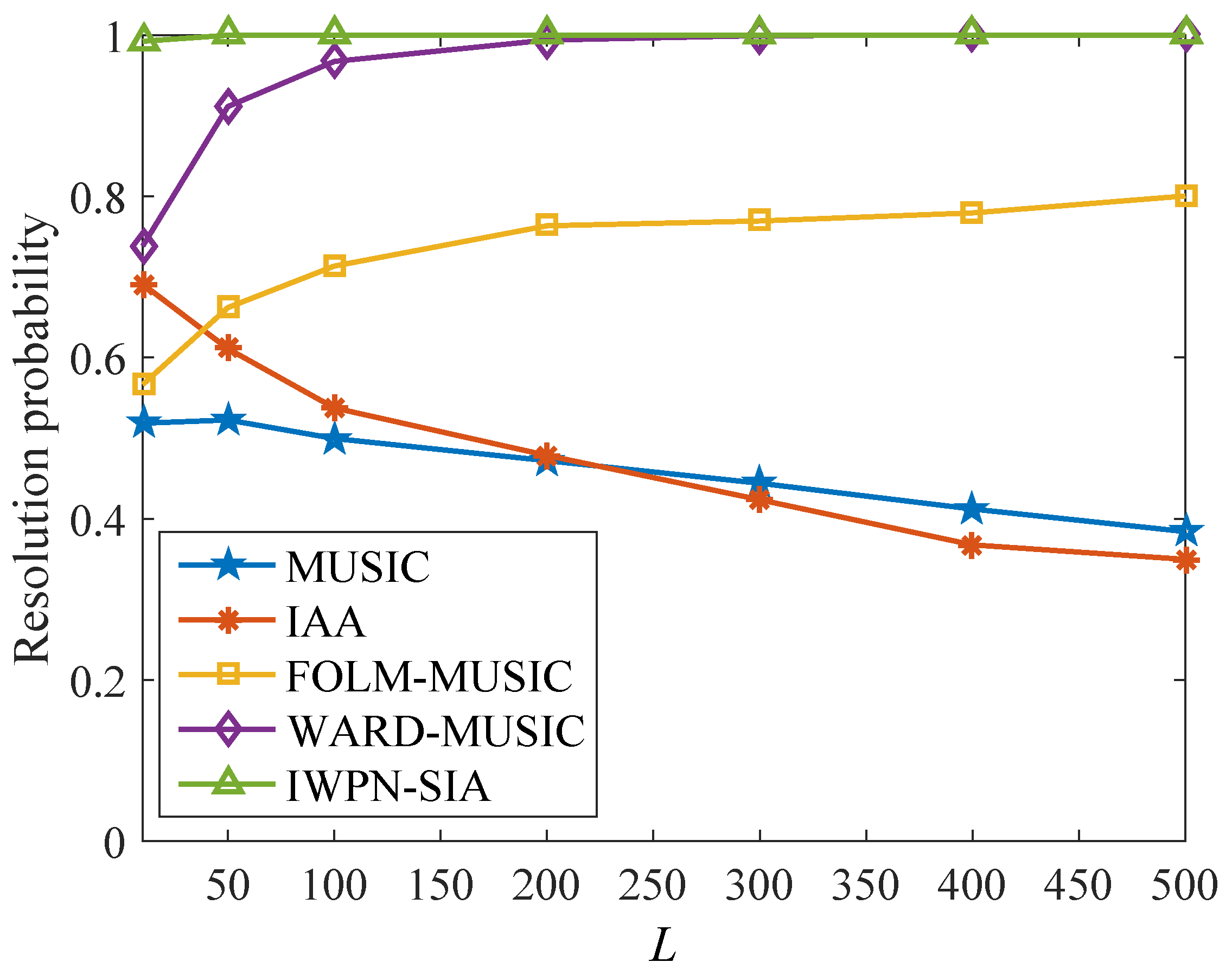
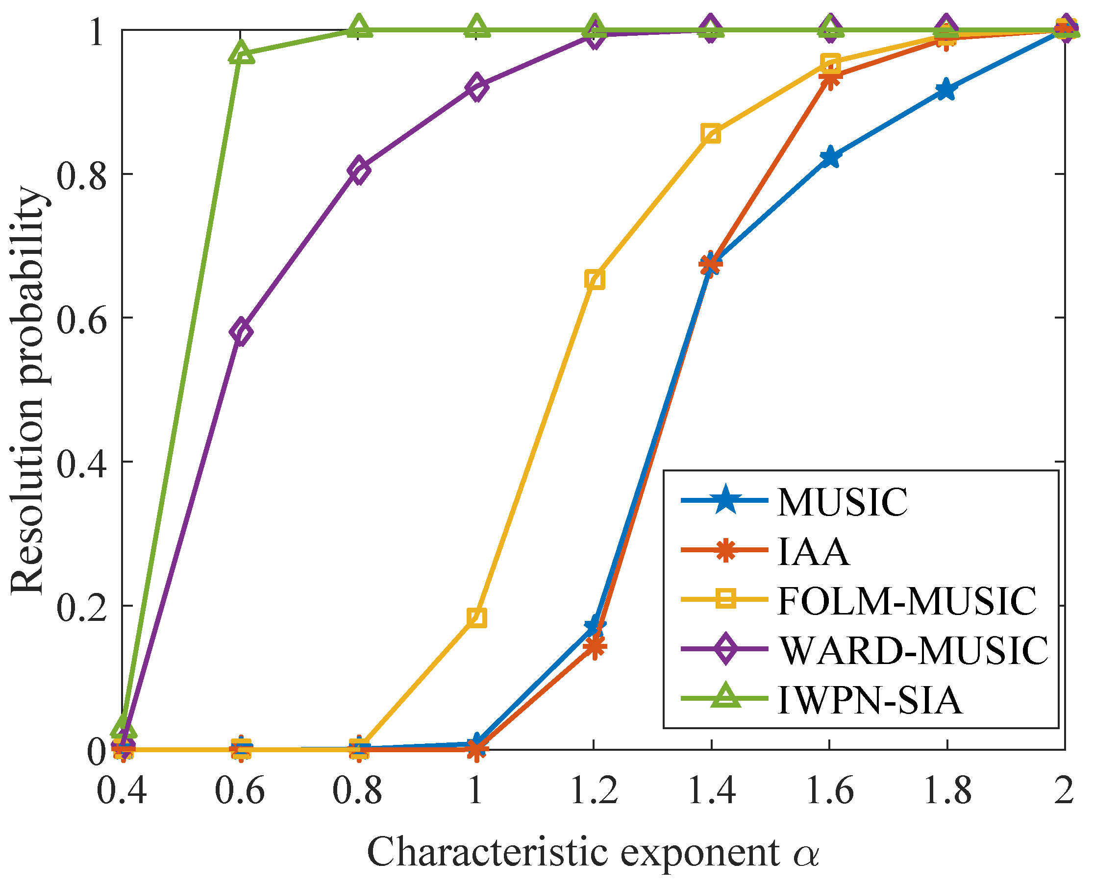
4.2. Comparison of the Resolution Probability

In this subsection, we compared the resolution probability of these algorithms from three aspects of GSNR, snapshots, and characteristic exponent $\alpha$.

Resolution probability over GSNR with $\alpha =1.3$ and $L=300$ can be seen in Figure 4. It is noticeable that the resolution probability of MUSIC and IAA methods cannot reach 100% with the gradual rise of GSNR, mainly due to the fact that both MUSIC and IAA methods are the DOA prediction techniques built on the Gaussian noise model. On the contrary, FLOM-MUSIC can effectively enhance the resolution probability by obtaining the covariance matrix through low-order processing. Furthermore, the performance of WARD-MUSIC is significantly improved by successively weighting snapshots to remove outliers and can achieve a resolution probability of 100% when the GSNR is not less than 6 dB. In general, the performance of IWPN-SIA, which combines outlier suppression and low-order processing, is significantly better than that of FLOM-MUSIC and WARD-MUSIC, and it is obvious that the proposed IWPN-SIA paradigm is able to attain a resolution likelihood of 100% when the GSNR is not less than 0 dB. This reveals that the proposed IWPN-SIA method has a higher resolution probability at low GSNR regions compared to other conventional methods.

In Figure 4, it can be seen that the proposed IWPN-SIA method has a high resolution probability when the DOA values of the signal sources are placed onto the discrete values of the angle grid, considering the fact that the aggregate signal will no longer be sparse in the grid domain if the DOAs are not placed onto the discrete values of the grid. To illustrate the impact of the DOAs not being on the grid on the performance, the result is given in Figure 5, where the DOAs of the incident waves are set to $60.5^{\circ }$ and $134.1^{\circ }$, and the other parameter settings remaining consistent. It can be seen from Figure 5 that compared to the DOAs of the signal on the grid, the resolution probability of the IWPN-SIA and WARD-MUSIC methods can still reach 100% when GSNR $\ge 0$ dB and GSNR $\ge 6$ dB, respectively, but their resolution probability is reduced when GSNR $<0$ dB and GSNR $<6$ dB, respectively. The resolution probability of other compared methods is decreased throughout the entire GSNR range when the DOAs of the signal are not placed onto the discrete values of the grid.

To validate the potency of the designed IWPN-SIA method with a reduced quantity of snapshots, we compare the resolution probability of the above mentioned techniques across varying numbers of snapshots, ranging from 10 to 500, with the GSNR static at 6 dB, and the remaining coefficients being kept constant with Figure 4. The resolution probability results of these algorithms are presented in Figure 6, where it can be noticed that the resolution probability of the MUSIC and IAA algorithms shows a decreasing trend as the amount of snapshots extends. The reason is that the quantity of outliers increases with the number of snapshots received in the impulsive noise atmosphere, significantly impacting the resolution capability of these algorithms based on Gaussian assumptions. Although the resolution probability of the FLOM-MUSIC, WARD-MUSIC, and IWPN-SIA methods has been increased with the rise in snapshot quantity, the suggested IWPN-SIA method has the highest resolution probability in the whole snapshot region, and its resolution performance is particularly significant compared to other methods in small snapshots.

The characteristic exponent $\alpha$ is an essential parameter of $\alpha$-stable dispersion, which has the ability to measure the strength of impulsive noise. Figure 7 depicts the resolution probability of these methods versus the characteristic exponent $\alpha$ where $\alpha$ ranges from 0.4 to 2, $L=300$, and the other parameters remain the same as Figure 6. It is noticed that the resolution accuracy of these techniques improves as $\alpha$ rises. The MUSIC, IAA, and FLOM-MUSIC methods fail when $\alpha <1$. In contrast to the MUSIC, IAA, and FLOM-MUSIC algorithms, while the resolution probability of the WARD-MUSIC and IWPN-SIA methods is significantly improved when $0.4<\alpha <1$, the proposed IWPN-SIA method still has a superior resolution probability compared to WARD-MUSIC.

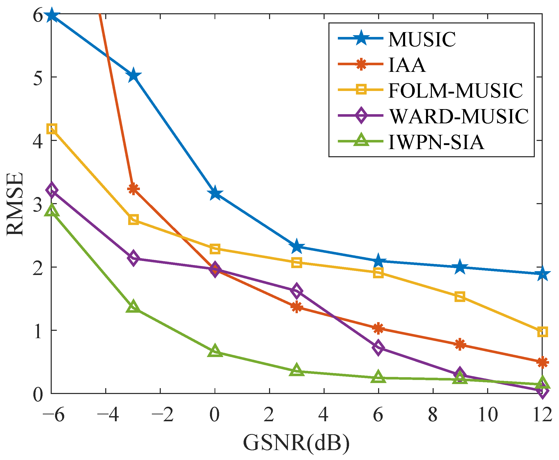
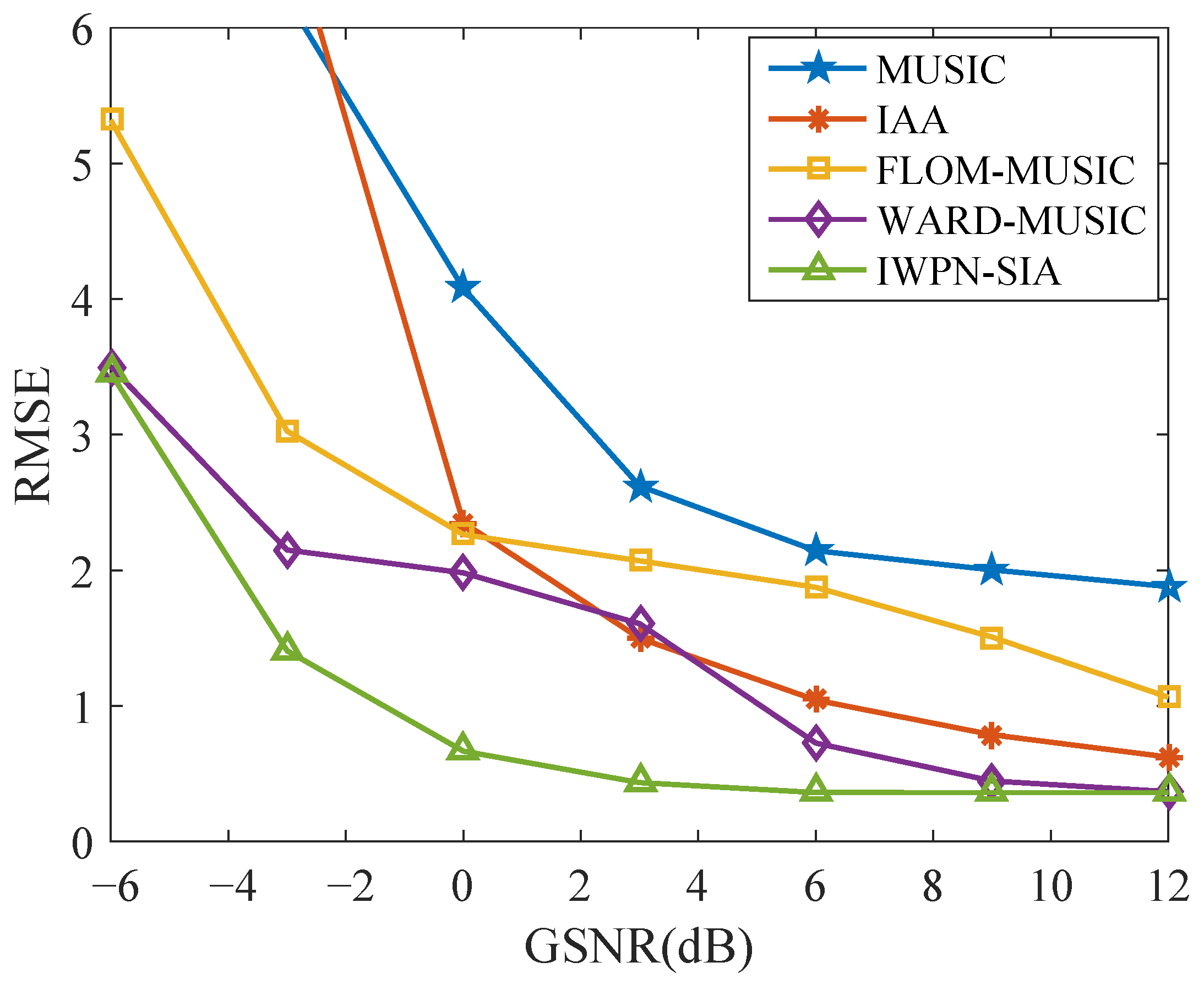
4.3. Comparison of RMSE

Here, we simulate the RMSE of the designed method and the comparison methods mentioned above from three aspects, including GSNR, snapshots, and the characteristic exponent $\alpha$.

The RMSEs of DOA estimates with $\alpha =1.3$ and $L=300$ are shown in Figure 8. It is obvious that the RMSE efficiency of IAA and MUSIC algorithms is poor, especially at the points when GSNR is low. This reveals that the impulsive noise has a serious impact on their DOA estimation performance. Although the RMSE of FLOM-MUSIC, WARD-MUSIC, and IWPN-SIA has improved in the case of low GSNR, the approximation precision of the designed IWPN-SIA algorithm is the highest in the given GSNR region.

We similarly consider the impact of the off-grid case on the RMSE. The DOAs of the incident wave are set to $60.5^{\circ }$ and $134.1^{\circ }$, and the other parameter settings are consistent with Figure 8; the result is shown in Figure 9. It can be seen that compared to Figure 8, the RMSE of all compared methods has increased, especially in areas with low GSNR, but the performance of the proposed IWPN-SIA method is the best.

For the purpose of assessing the effectiveness of the designed IWPN-SIA technique when dealing with small snapshots, Figure 10 shows the effect of the value of snapshots, where the GSNR is fixed to 6 dB and other parameters remain consistent with Figure 8, from which it can be observed that as the volume of snapshots rises, the RMSE of the MUSIC and IAA techniques no longer declines. This also indicates that the impulsive noise has a meaningful impact on their estimation behavior. Although the RMSE of the FLOM-MUSIC, WARD-MUSIC, and IWPN-SIA methods increases with the number of snapshots, their RMSEs are never lower than that of IWPN-SIA. Even under small snapshot conditions, the proposed IWPN-SIA algorithm continues to exhibit superior estimation performance.

The comparison of different parameters indicates that the effectiveness of the proposed IWPN-SIA techniques is far better than the existing methodologies. When examining the RMSE of all techniques regarding characteristic parameter $\alpha$, $\alpha$ ranges from 0.4 to 2, $L=300$, and the other parameters remain the same as Figure 10; this is shown in Figure 11. It is worth noting that the $\alpha$-stable dispersion gradually tends to the Gaussian spread with the increase of $\alpha$. As a result, the estimation accuracy of each compared method is significantly enhanced. Clearly, the MUSIC, IAA, and FLOM-MUSIC methods have high RMSE when $\alpha <1$. In contrast, the RMSE of the WARD-MUSIC and IWPN-SIA methods is significantly lower than MUSIC and IAA methods when $0.4<\alpha <1$. Although the DOA prediction accuracy of MUSIC, IAA, and WARD-MUSIC methods is higher than the designed IWPN-SIA algorithm when $\alpha =2$, the proposed IWPN-SIA method has the lowest RMSE when $\alpha <2$.

5. Conclusions

In this study, DOA approximation of AVSA in the presence of impulsive noise is explored. Combining the outlier handling method and the low-order processing method, an IWPN-SIA algorithm is proposed to overcome this issue. Taking advantage of the significant difference between outliers and common data values, the weighted infinite norm method is used to suppress the impact of high outliers. Then, a new fitness criterion is formulated to address the impulse characteristics of the residual, and then the systematic function for the power of sparse signal is formed. Finally, the DOA is determined by performing a spectral peak search on the sparse signal power. Simulation results show that the estimation performance of the MUSIC and IAA methods is severely degraded when they are applied to AVSA for DOA estimation in the presence of impulsive noise. Although the FLOM-MUSIC, WARD-MUSIC, and IWPN-SIA methods can effectively suppress impulsive noise, the estimation performance of the proposed IWPN-SIA method is improved by approximately 12 dB and 6 dB compared with FLOM-MUSIC and WARD-MUSIC, respectively, under the same resolution probability. In addition, the proposed IWPN-SIA algorithm shows superior performance in small snapshots and intense impulsive noise. However, in this paper, the proposed IWPN-SIA method only considers the case of impulsive noise. It is worth noting that the types of noise are usually complex in practical underwater environments, such as non-uniform noise, colored noise, Gaussian and non-Gaussian mixed noise, etc. These types of noise would seriously affect the DOA estimation performance of the proposed IWPN-SIA method. In future work, we will investigate the impact of different noise types on the DOA estimation performance of AVSA and propose improved methods.

References

1. Abraham, B.M. Ambient noise measurements with vector acoustic hydrophones. In Proceedings of the OCEANS 2006, Boston, MA, USA, 18–21 September 2006; pp. 1–7. [Google Scholar] [CrossRef]
2. Nagananda, K.; Anand, G. Underwater target tracking with vector sensor array using acoustic field measurements. In Proceedings of the OCEANS 2017-Aberdeen, Aberdeen, UK, 19–22 June 2017; pp. 1–10. [Google Scholar] [CrossRef]
3. Gunes, A.; Guldogan, M.B. Joint underwater target detection and tracking with the Bernoulli filter using an acoustic vector sensor. Digit. Signal Process. 2016, 48, 246–258. [Google Scholar] [CrossRef]
4. Zhang, L.; Wu, D.; Han, X.; Zhu, Z. Feature extraction of underwater target signal using mel frequency cepstrum coefficients based on acoustic vector sensor. J. Sensors 2016, 2016, 7864213. [Google Scholar] [CrossRef]
5. Han, X.; Yin, J.; Yu, G.; Du, P. Experimental demonstration of single carrier underwater acoustic communication using a vector sensor. Appl. Acoust. 2015, 98, 1–5. [Google Scholar] [CrossRef]
6. Zhao, A.; Ma, L.; Hui, J.; Liu, L. Research and implementation of bistatic sonar positioning system based on vector hydrophone. In Proceedings of the 2016 IEEE/OES China Ocean Acoustics (COA), Harbin, China, 9–11 January 2016; pp. 1–5. [Google Scholar] [CrossRef]
7. Bozzi, F.d.A.; Jesus, S.M. Vector sensor beam steering for underwater acoustic communications. Proc. Meet. Acoust. 2020, 42, 070002. [Google Scholar] [CrossRef]
8. Raghukumar, K.; Chang, G.; Spada, F.; Jones, C. A vector sensor-based acoustic characterization system for marine renewable energy. J. Mar. Sci. Eng. 2020, 8, 187. [Google Scholar] [CrossRef]
9. Santos, P.; Rodríguez, O.; Felisberto, P.; Jesus, S. Seabed geoacoustic characterization with a vector sensor array. J. Acoust. Soc. Am. 2010, 128, 2652–2663. [Google Scholar] [CrossRef] [PubMed]
10. Najeem, S.; Kiran, K.; Malarkodi, A.; Latha, G. Open lake experiment for direction of arrival estimation using acoustic vector sensor array. Appl. Acoust. 2017, 119, 94–100. [Google Scholar] [CrossRef]
11. Nehorai, A.; Paldi, E. Acoustic vector-sensor array processing. IEEE Trans. Signal Process. 1994, 42, 2481–2491. [Google Scholar] [CrossRef]
12. Schmidt, R. Multiple emitter location and signal parameter estimation. IEEE Trans. Antennas Propag. 1986, 34, 276–280. [Google Scholar] [CrossRef]
13. Wong, K.T.; Zoltowski, M.D. Extended-aperture underwater acoustic multisource azimuth/elevation direction-finding using uniformly but sparsely spaced vector hydrophones. IEEE J. Ocean. Eng. 1997, 22, 659–672. [Google Scholar] [CrossRef]
14. Kundu, D. Modified MUSIC algorithm for estimating DOA of signals. Signal Process. 1996, 48, 85–90. [Google Scholar] [CrossRef]
15. Zhang, Y.; Ng, B.P. MUSIC-like DOA estimation without estimating the number of sources. IEEE Trans. Signal Process. 2009, 58, 1668–1676. [Google Scholar] [CrossRef]
16. Meng, X.; Cao, B.; Yan, F.; Greco, M.; Gini, F.; Zhang, Y. Real-Valued MUSIC for Efficient Direction of Arrival Estimation with Arbitrary Arrays: Mirror Suppression and Resolution Improvement. Signal Process. 2023, 202, 108766. [Google Scholar] [CrossRef]
17. Bensalem, M.; Barkat, O. DOA estimation of linear dipole array with known mutual coupling based on ESPRIT and MUSIC. Radio Sci. 2022, 57, 1–15. [Google Scholar] [CrossRef]
18. Malioutov, D.; Cetin, M.; Willsky, A. A sparse signal reconstruction perspective for source localization with sensor arrays. IEEE Trans. Signal Process. 2005, 53, 3010–3022. [Google Scholar] [CrossRef]
19. Hawkes, M.; Nehorai, A. Acoustic vector-sensor correlations in ambient noise. IEEE J. Ocean. Eng. 2001, 26, 337–347. [Google Scholar] [CrossRef]
20. Shi, S.; Li, Y.; Yang, D.; Liu, A.; Shi, J. Sparse representation based direction-of-arrival estimation using circular acoustic vector sensor arrays. Digit. Signal Process. 2020, 99, 102675. [Google Scholar] [CrossRef]
21. Shi, S.; Li, Y.; Yang, D.; Liu, A.; Zhu, Z. DOA estimation of coherent signals based on the sparse representation for acoustic vector-sensor arrays. Circuits Syst. Signal Process. 2020, 39, 3553–3573. [Google Scholar] [CrossRef]
22. Yardibi, T.; Li, J.; Stoica, P.; Xue, M.; Baggeroer, A. Source localization and sensing: A nonparametric iterative adaptive approach based on weighted least squares. IEEE Trans. Aerosp. Electron. Syst. 2010, 46, 425–443. [Google Scholar] [CrossRef]
23. Wang, W.; Tan, W.; Li, H.; Zhang, Q.; Shi, W. Source localization utilizing weighted power iterative compensation via acoustic vector hydrophone array. Appl. Acoust. 2021, 182, 108228. [Google Scholar] [CrossRef]
24. Wang, W.; Tan, W.; Shi, W.; Zhang, Q.; Li, H. Direction finding based on iterative adaptive approach utilizing weighted l2-norm penalty for acoustic vector sensor array. Multidimens. Syst. Signal Process. 2022, 33, 247–261. [Google Scholar] [CrossRef]
25. Blackard, K.L.; Rappaport, T.S.; Bostian, C.W. Measurements and models of radio frequency impulsive noise for indoor wireless communications. IEEE J. Sel. Areas Commun. 1993, 11, 991–1001. [Google Scholar] [CrossRef]
26. Brockett, P.L.; Hinich, M.; Wilson, G.R. Nonlinear and non-Gaussian ocean noise. J. Acoust. Soc. Am. 1987, 82, 1386–1394. [Google Scholar] [CrossRef]
27. Dong, Y.; Dong, C.; Liu, W.; Cai, J. Generalized 2-p minimization based DOA estimation for sources with known waveforms in impulsive noise. Signal Process. 2022, 190, 108313. [Google Scholar] [CrossRef]
28. Kozick, R.J.; Sadler, B.M. Maximum-likelihood array processing in non-Gaussian noise with Gaussian mixtures. IEEE Trans. Signal Process. 2000, 48, 3520–3535. [Google Scholar] [CrossRef]
29. Wen, F.; Liu, P.; Liu, Y.; Qiu, R.C.; Yu, W. Robust Sparse Recovery in Impulsive Noise via p-1 Optimization. IEEE Trans. Signal Process. 2016, 65, 105–118. [Google Scholar] [CrossRef]
30. Liu, M.; Zhang, J.; Tang, J.; Jiang, F.; Liu, P.; Gong, F.; Zhao, N. 2-D DOA robust estimation of echo signals based on multiple satellites passive radar in the presence of alpha stable distribution noise. IEEE Access 2019, 7, 16032–16042. [Google Scholar] [CrossRef]
31. Chen, S.; Gu, F.; Liang, C.; Meng, H.; Wu, K.; Zhou, Z. Review on Active Noise Control Technology for α-Stable Distribution Impulsive Noise. Circuits Syst. Signal Process. 2022, 41, 956–993. [Google Scholar] [CrossRef]
32. Meng, H.; Chen, S. A modified adaptive weight-constrained FxLMS algorithm for feedforward active noise control systems. Appl. Acoust. 2020, 164, 107227. [Google Scholar] [CrossRef]
33. Tsakalides, P.; Nikias, C.L. The robust covariation-based MUSIC (ROC-MUSIC) algorithm for bearing estimation in impulsive noise environments. IEEE Trans. Signal Process. 1996, 44, 1623–1633. [Google Scholar] [CrossRef]
34. Liu, T.H.; Mendel, J.M. A subspace-based direction finding algorithm using fractional lower order statistics. IEEE Trans. Signal Process. 2001, 49, 1605–1613. [Google Scholar] [CrossRef]
35. Belkacemi, H.; Marcos, S. Robust subspace-based algorithms for joint angle/Doppler estimation in non-Gaussian clutter. Signal Process. 2007, 87, 1547–1558. [Google Scholar] [CrossRef]
36. He, J.; Liu, Z. WARD: A weighted array data scheme for subspace processing in impulsive noise. In Proceedings of the 2006 IEEE International Conference on Acoustics Speech and Signal Processing Proceedings, Toulouse, France, 14–19 May 2006; pp. 1049–1052. [Google Scholar] [CrossRef]
37. Li, S.; He, R.; Lin, B.; Sun, F. DOA estimation based on sparse representation of the fractional lower order statistics in impulsive noise. IEEE/CAA J. Autom. Sin. 2016, 5, 860–868. [Google Scholar] [CrossRef]
38. Hu, R.; Fu, Y.; Chen, Z.; Xu, J.; Tang, J. Robust DOA estimation via sparse signal reconstruction with impulsive noise. IEEE Commun. Lett. 2017, 21, 1333–1336. [Google Scholar] [CrossRef]
39. Ma, F.; Xu, C.; Zhang, X.; He, J.; Su, W. Iterative reweighted DOA estimation for impulsive noise processing based on off-grid variational Bayesian learning. IEEE Access 2019, 7, 104642–104654. [Google Scholar] [CrossRef]
40. Guo, M.; Sun, Y.; Dai, J.; Chang, C. Robust DOA estimation for burst impulsive noise. Digit. Signal Process. 2021, 114, 103059. [Google Scholar] [CrossRef]
41. Jian, L.; Wang, X.; Shi, J.; Lan, X. Robust Sparse Bayesian Learning Scheme for DOA Estimation with Non-Circular Sources. Mathematics 2022, 10, 923. [Google Scholar] [CrossRef]
42. Rong, J.; Zhang, J.; Duan, H. Robust sparse Bayesian learning based on the Bernoulli-Gaussian model of impulsive noise. Digit. Signal Process. 2023, 136, 104013. [Google Scholar] [CrossRef]
43. Chen, D.; Joo, Y.H. Multisource DOA Estimation in Impulsive Noise Environments Using Convolutional Neural Networks. Int. J. Antennas Propag. 2022, 2022, 5325076. [Google Scholar] [CrossRef]
44. Liang, L.; Shi, Y.; Shi, Y.; Bai, Z.; He, W.; Lv, X. Off-grid sparse based two-dimensional direction of arrival estimation of acoustic vector sensor array in impulse noise. Noise Vib. Worldw. 2022, 53, 480–486. [Google Scholar] [CrossRef]
45. Tian, Q.; Qiu, T.; Cai, R. DOA estimation for CD sources by complex cyclic correntropy in an impulsive noise environment. IEEE Commun. Lett. 2020, 24, 1015–1019. [Google Scholar] [CrossRef]
46. Gong, J.; Guo, Y. A bistatic MIMO radar angle estimation method for coherent sources in impulse noise background. Wirel. Pers. Commun. 2021, 116, 3567–3576. [Google Scholar] [CrossRef]
47. Jennings, A.; McKeown, J.J. Matrix Computation; John Wiley & Sons Inc.: Hoboken, NJ, USA, 1992. [Google Scholar]
48. Haagerup, U. Lp-Spaces Associated with an ARBITRARY von Neumann Algebra. Algebres d’Opérateurs et Leurs Applications en Physique Mathématique. 1977, pp. 175–184. Available online: https://dmitripavlov.org/scans/haagerup.pdf (accessed on 30 July 2023).
Figure 1. The AVS uniform linear array.
Jmse 11 01798 g001
Figure 2. Resolution probability versus p.
Jmse 11 01798 g002
Figure 3. RMSE versus p.
Jmse 11 01798 g003
Figure 4. Resolution probability versus GSNR with θ 1 = 60 , θ 2 = 134 .
Jmse 11 01798 g004
Figure 5. Resolution probability versus GSNR with θ 1 = 60 . 5 , θ 2 = 134 . 1 .
Jmse 11 01798 g005
Figure 6. Resolution probability versus L.
Jmse 11 01798 g006
Figure 7. Resolution probability versus the characteristic exponent α .
Jmse 11 01798 g007
Figure 8. RMSE versus GSNR with θ 1 = 60 , θ 2 = 134 .
Jmse 11 01798 g008
Figure 9. RMSE versus GSNR with θ 1 = 60 . 5 , θ 2 = 134 . 1 .
Jmse 11 01798 g009
Figure 10. RMSE versus L.
Jmse 11 01798 g010
Figure 11. RMSE versus the characteristic exponent α .
Jmse 11 01798 g011
Disclaimer/Publisher’s Note: The statements, opinions and data contained in all publications are solely those of the individual author(s) and contributor(s) and not of MDPI and/or the editor(s). MDPI and/or the editor(s) disclaim responsibility for any injury to people or property resulting from any ideas, methods, instructions or products referred to in the content.