Characterization of Abrasive Grain Signal of Oil Detection Sensor Based on LC Resonance Wireless Transmission

Abstract

Friction in marine engineering machinery produces abrasive particles containing valuable information. By employing oil detection technology, we can analyze these particles to monitor and diagnose mechanical system faults. This paper introduces an inductive oil detection sensor and wireless signal transmission circuit. The sensor utilizes two opposing solenoid coils of the same specifications, with the detection coil connected to a chip capacitor to form an LC resonant unit. The designed wireless transmission circuit wirelessly transmits a sensing signal from a detection coil to a receiving coil to detect metal particles in oil. This paper deduces the sensor’s inductance principle and simulates the magnetic field distribution using finite element simulation software. Through experiments, the optimal excitation frequency, coil spacing, and oil sample flow path location were determined. The sensor successfully detected 55 μm iron particles and 138 μm copper particles in a 1 mm microfluidic channel. With its simple structure, distinct signal characteristics, and high sensitivity, the sensor is suitable for detecting metal abrasive particles in hydraulic oil, providing a new approach for wireless transmission in oil detection sensors.

1. Introduction

The importance of lubricating oil in marine engineering machinery and equipment cannot be ignored. Lubricating oil can reduce the friction between machine and equipment parts, prevent their wear and damage, and extend the service life of the machine and equipment. At the same time, the lubricant can also help the machine and equipment to realize more efficient operation through the role of energy transfer. In a high-temperature environment, lubricating oil also has the role of cooling, to maintain the normal working temperature of the machines and equipment. In addition, the lubricant can also play a sealing role, to prevent gas and liquid leakage inside the equipment and machine. Ship equipment and wind power equipment are examples. When a ship’s internal combustion engine is operating without adequate lubrication, phenomena such as dry friction may occur, and the heat generated by dry friction has a high probability of melting the metal. The melting of equipment parts can be fatal to ship safety. There are also certain gaps between the engine’s cylinders and pistons and piston rings to ensure the smooth operation of the components, but due to these gaps, the cylinders may suffer from poor sealing. The oil film formed by the lubricant in these gaps ensures that the cylinders are adequately sealed, thereby maintaining the cylinder pressure to ensure the output power of the internal combustion engine. At the same time, there are many ships with hydraulic oil as the medium for hydraulic equipment, such as servo systems, cranes, hydraulic pumps, hydraulic valves and other equipment. Because hydraulic oil is not easily compressed, it is often used to transmit power or control the equipment of a ship remotely. Lubricants also play an important role in wind power equipment. For gearboxes and bearings, lubricant reduces friction in gearboxes and bearings, thereby reducing wear between components. It also reduces the shock forces from the gearboxes and bearings, which reduces equipment vibration. Lubricants are also used in the hydraulic systems of wind turbines. The wind turbine drive chain brakes as well as the yaw braking system are driven by the hydraulic system of the wind turbine. This lubricant also prevents oxidization of components in marine equipment and wind turbines. Therefore, lubricating oil is an indispensable and significant medium in marine engineering machinery and equipment [1]. During the operation of the ship’s equipment, many metal particles are generated due to friction between parts and other factors, and these particles will enter the oil fluid and be distributed to the whole equipment with the flow of the hydraulic system and lubrication system. It can be seen that the detection of microscopic particles in the ship’s oil can effectively monitor the wear and tear between the ship’s components, so as to carry out targeted maintenance of the ship’s equipment, which is very important for the normal navigation of ships. Similarly, the health of wind turbine gearboxes and bearings can be monitored by detecting oil particles. To accurately and efficiently monitor wear particles in the oil, researchers have developed a variety of online and offline oil sensors. Optical methods are one of the commonly used techniques that can detect attributes such as geometry, size, and coloration of wear particles [2,3,4]. However, optical methods [5] require a high level of fluid cleanliness and are usually only suitable for laboratory testing [6]. The acoustic method is another widely used method with sensors capable of accurately detecting wear particles in the oil. In contrast to optical sensors, fluid cleanliness does not affect the operation of acoustic sensors, so acoustic sensors can operate at high levels of detection accuracy [7]. However, acoustic methods are less resistant to external sound and vibration interference, and therefore require appropriate suppression measures in practical applications [8,9,10]. The capacitance method is also highly sensitive for detecting tiny substances in oil fluids, such as water droplets and air bubbles. Through the application of capacitance method sensors, the purity and moisture content of the oil can be monitored in real time. However, it is important to recognize that the capacitance method is unable to distinguish between ferromagnetic and non-ferromagnetic particles, and therefore may not provide accurate differentiation results when detecting wear particles in oil fluids [11,12,13].

The inductive method is a commonly used method for detecting wear particles in oil. Current research has focused on two main areas: improving the detection sensitivity of the sensor to recognize smaller-sized wear particles and making the sensor suitable for online detection. To increase the sensitivity of the sensor, researchers used the microfluidic technique [14], where the sensor’s oil flow path is placed in a high-gradient magnetic field. This approach allows the sensor to have very high detection sensitivity. However, due to the low detection flux of the microfluidic channel, there is a problem that can easily lead to clogging of wear particles [15]. In marine hydraulic systems, the size of wear particles in the hydraulic fluid should normally be less than 20 μm. However, once abnormal operation of the equipment occurs, the size of wear particles may increase rapidly to more than 50 μm [16,17]. Therefore, improving the detection sensitivity of the sensors has become a key issue for research [18,19,20]. Some studies have formed parallel detection sequences of multiple microfluidic sensors by applying techniques such as frequency-division multiplexing and time-division multiplexing to maintain the high sensitivity of the sensors while improving the detection throughput [21]. However, this approach still needs to address the problem of the large size of individual microfluidic channels. In addition, there are some studies that sought to improve the detection sensitivity by using an inductive coil as the bridge arm based on the bridge balance theory and utilizing the principle that metal abrasive particles cause damage to the bridge balance [22], and the signal is processed by the subsequent conditioning circuit.

At present, research on inductive oil detection sensors primarily focuses on enhancing detection sensitivity and improving detection throughput [23,24]. To solve these problems, a medium-sized inductive wireless transmission oil detection sensor is designed in this paper. The sensor adopts the structure of two electromagnetic coils of the same size placed opposite to each other and forms an LC resonant circuit by connecting the detection coil with a chip capacitor. Wireless detection of metal particles in the oil circuit can be realized by reading the changes in the inductive characteristics of the LC resonant circuit with a wireless receiver coil. In addition, the sensor improves contaminant detection accuracy, compared to other microfluidic sensors, and the designed sensor can achieve higher detection accuracy. Meanwhile, the magnetic field inside the sensor is relatively homogeneous, which reduces the detection error. In this research, the sensor was analyzed for wireless transmission through theoretical derivation, and the magnetic field distribution of the sensor structure was simulated using finite element simulation software. In addition, experiments were conducted to explore the optimal excitation frequency of the sensor, resulting in the determination of the lower detection limit for metallic abrasive particles; the influence of the spacing between the two electromagnetic coils of this sensor and the optimal oil sample flow path location were analyzed. These findings lay the foundation for long-distance detection of oil contaminants.

Overall, the inductive wireless transmission oil detection sensor designed in this paper has high detection sensitivity and detection throughput and can be adapted to online detection. The design and performance of this sensor will be further optimized in the future as needed to better meet the practical application requirements. This work is compared with other work as shown in

Table 1. Comparison of our sensor to other sensors.

Principle	Advantage	Disadvantage
optical methods [2,3,4]	Can detect attributes such as geometry, size, and coloration of wear particles	Require a high level of fluid cleanliness
acoustic method [7]	Fluid cleanliness does not affect the operation of acoustic sensors	Less resistant to external sound and vibration interference
capacitance method [11,12,13]	The purity and moisture content of the oil can be monitored in real-time	Unable to distinguish between ferromagnetic and non-ferromagnetic particles
inductive method [14]	Can distinguishbetween ferromagnetic and non-ferromagnetic metal particles	Can easily lead to clogging of wear particles/needs to address the problem of the large size of individual microfluidic channels
this work	Can increase the detection flux without decreasing the detection sensitivity	Cannot distinguish between water and air bubbles

.

2. Sensor Design and Principle

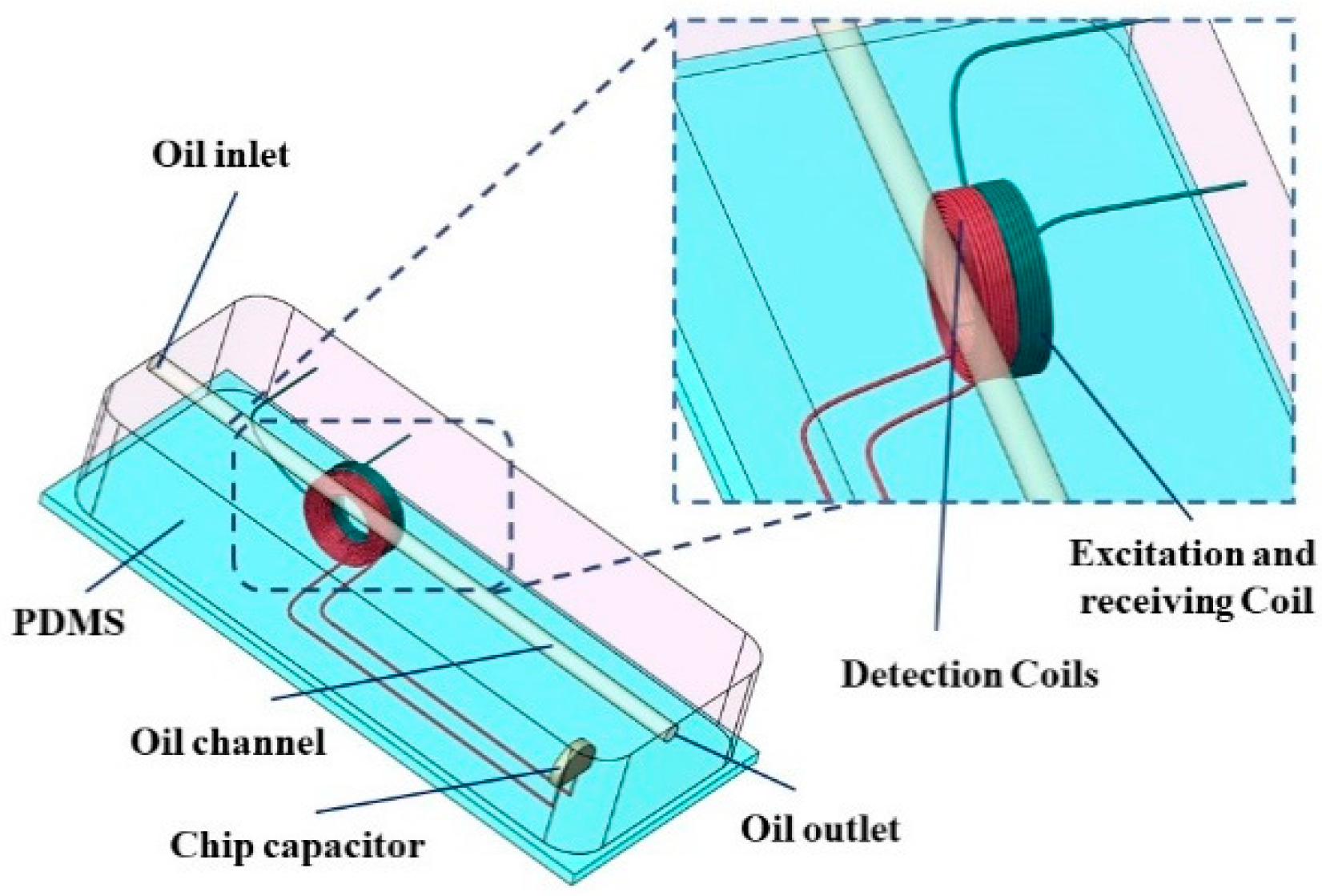
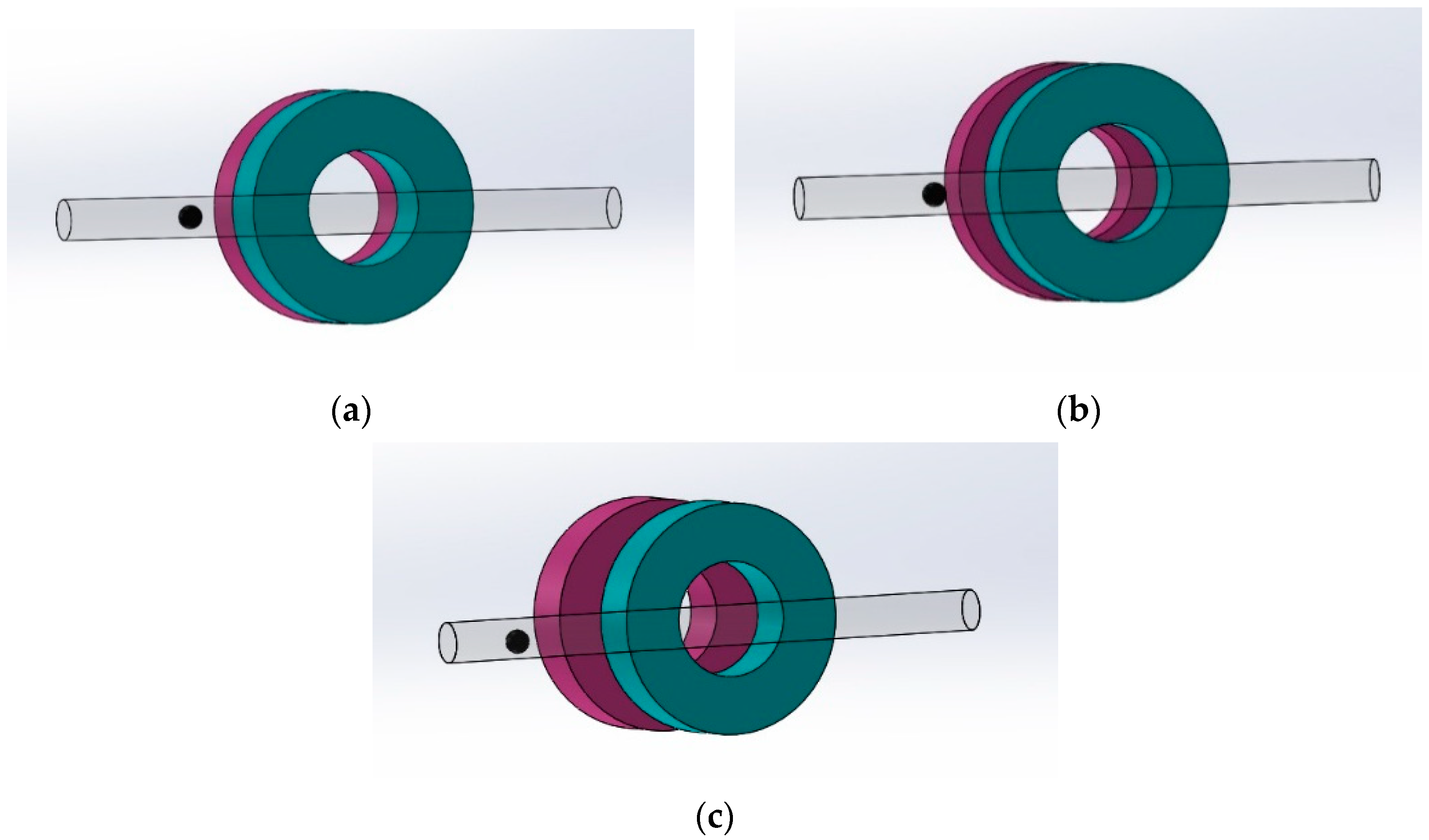
2.1. Sensor Design

The sensor design is shown in Figure 1. A dual-coil structure was used, with the green coil as the excitation and reception coil and the purple color as the detection coil. The two coils were placed opposite one another. The excitation and detection coils were both wound with 200 turns of coil, with an inner diameter of 2 mm, an outer diameter of 4 mm, a height of 1 mm, and a wire diameter of 0.05 mm. An oil channel was arranged around the edge of the detection coil for the oil to be measured to pass through. A copper rod with a diameter of 1 mm was selected and fixed on the side of the coil to create a microfluidic channel for the oil sample to pass through after pouring, and the fabricated components were neatly arranged in an open square mold. Using the plastic molding method, PDMS (Polydimethylsiloxane) and a curing agent were mixed into a gel at a ratio of 10:1, poured into the square mold, placed in a drying oven, and heated for 30 min for curing. Finally, the cured sensor was wrapped with aluminum foil to shield the sensor from external electromagnetic interference and complete the sensor. Among them, the detection coil was connected to the chip capacitor to form an LC resonant circuit. In the experiment, we placed the detection coil inside the pipe, and the signal of contaminants in the oil was read wirelessly by the receiving coil, so as to detect the metal wear particles in the pipeline.

When ferromagnetic particles pass through the detection area of the sensor, the magnetization effect from the high permeability increases the inductance of the coil, producing an upward inductive signal. In contrast, when nonferromagnetic metal particles pass through the sensor’s detection area, the eddy current effect is stronger, resulting in a decrease in the coil inductance and a downward inductance signal. Thus, ferromagnetic and non-ferromagnetic particles can be distinguished by an increase or decrease in the inductive signal, while the number of metal particles can be inferred from the number of peaks. As the size of the particles increases, the magnitude of the change in the inductance signal increases, so the approximate size of the metal particles can be estimated.

2.2. Detection Principle

The sensor proposed in this paper consists of an excitation-reading coil, an LC resonant loop consisting of a detection coil, and a patch capacitor. The circuit model is shown in Figure 2.

The green dashed line frames the part that is both the excitation and receiving coil, and the blue dashed line frames the part that is the detecting coil. Among them, $L_1$ and $R_1$ are the inductance and resistance of the excitation and reception coils, respectively, and $L_2$, $R_2$ and $C_2$ are the inductance, resistance, and patch capacitance of the detection coil, respectively. In the design of this sensor, $L_1=L_2=97 \mathsf{\mu }\mathrm{H}$, $R_1=R_2=18.2 \mathsf{\Omega }$, and $C_2=330 \mathrm{PF}$. The resonant frequency of the sensor is determined by the values of the inductor $L_2$ and capacitor $C_2$ and is calculated as follows [25]:

$$f_0={\displaystyle \frac{1}{2\pi \sqrt{L_2{C}_2}}}$$

(1)

When the sensor operates, a frequency of f is applied to the excitation coil and, due to the coupling of the magnetic field, the detection coil generates an induced current with frequency f. To further analyze the effect of metal particles on the equivalent impedance $Zeq$ when passing through the sensor, the equivalent circuit model is first analyzed by using circuit analysis.

$$Z_{11}{I}_1+Z_M{I}_1=U_S$$

(2)

$$Z_{22}{I}_2+Z_M{I}_1=0$$

(3)

Among them, $I_1$ and $I_2$ are the input currents of the two coils, and $U_s$ is the excitation voltage of the circuit. $Z_{11}$ and $Z_{22}$ are the impedance values of the external readout coil and the internal resonant unit, respectively, and $Z_m$ is regarded as the mutual inductance impedance. The values are, respectively,

$$Z_{11}=R_1+j\omega L_1$$

(4)

$$Z_{22}=R_2+j\left(\omega L_2-{\displaystyle \frac{1}{\omega C_2}}\right)$$

(5)

$$Z_M=j\omega M$$

(6)

In the above equation, $\omega$ is the angular velocity of the alternating magnetic field, and its value is a function of the alternating current frequency $f$; $M$ is the mutual inductance between the inner and outer coils of the sensor, and its value is determined by the inductance value, shape, size, position, and other factors of the inner and outer coils. This can be seen from the sensor equivalent circuit model:

$$Z_{eq}=Z_{11}+R_z={\displaystyle \frac{U_S}{I_1}}$$

(7)

$$Z_{eq}=R_1+j\omega L_1+{\displaystyle \frac{{\omega }^2{M}^2}{R_2+j(\omega L_2-\frac{1}{\omega C_2})}}$$

(8)

Then, the inductance change is

$$\Delta L=I_m({\displaystyle \frac{\Delta Z}{\omega }})$$

(9)

$\omega$ is the angular frequency of the alternating magnetic field, and its value is a function of the alternating current frequency $f$. $I_m$ is the equivalent inductance. $\Delta Z$ is the change in the equivalent impedance of the sensor.

When ferromagnetic particles pass through the detection area, they are affected by magnetization and eddy current effects. In contrast, non-ferromagnetic particles do not undergo magnetization effects but do undergo eddy current effects. The eddy current effect refers to the block metal conductor placed in the changing magnetic field or in the magnetic field for cutting the lines of magnetic force of the block metal conductor. The block metal conductor will produce a vortex-like induced current in the phenomenon. For ferromagnetic particles, the inductance produced by its eddy current effect is very weak, while the inductance produced by the magnetization effect is very strong. Therefore, the change in the electromagnetic field of the ferromagnetic particles is mainly caused by the magnetization effect, and because the direction of the inductance of its magnetization effect is the same as the direction of the inductance of the magnetic field of the original coil, which leads to an increase in the inductance of the induction coil $L_2$, whereas the non-ferromagnetic particles are affected by the eddy current effect when they pass through, which produces an inductance in the opposite direction of the inductance direction of the original magnetic field, thus leading to the decrease in the inductance of the inductor coil $L_2$.

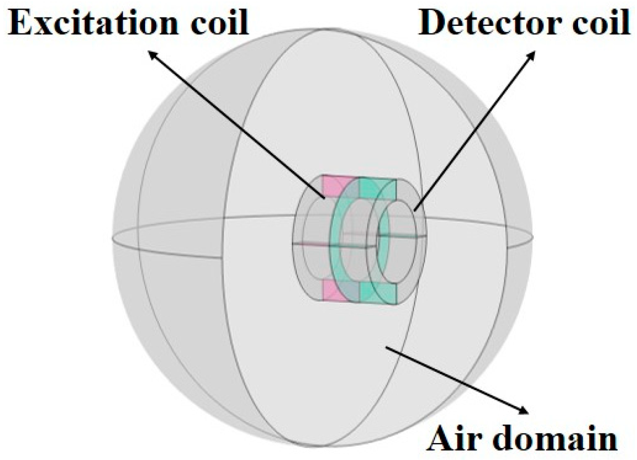
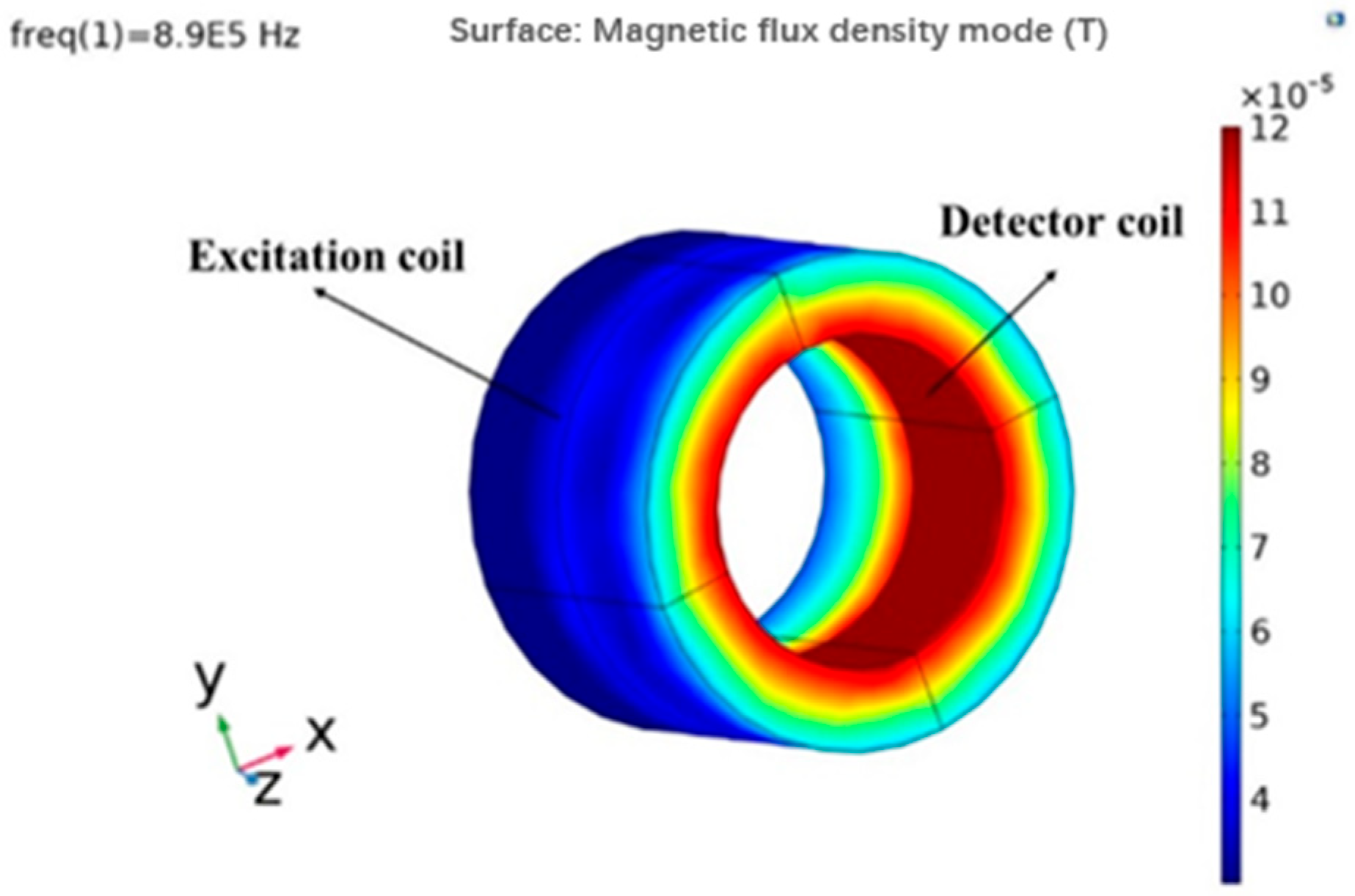
3. Finite Element Simulation

COMSOL is a commonly used finite element computational software for magnetic field analysis and provides a unique magnetic field module for solving problems involving magnetic and other physical fields [26].

In order to validate the sensor model, this paper develops a finite element model in COMSOL for obtaining the magnetic flux density modes at every position of the sensor. First, the purpose of choosing a magnetic field steady-state solver to calculate the magnetic field distribution around the coil is to study the magnetic field distribution around the sensor.

Secondly, in the modeling process, the actual parameters of the sensor were used to construct the simulation model, as shown in Figure 3. The simulation model of two 200-turn coils (2 mm inner diameter, 4 mm outer diameter, wound by 50 μm diameter copper wire) was built in the COMSOL6.0 software. The two coils were kept concentric and closely fit, and a 330 pF capacitive element was connected in series with the detecting coil to form an LC resonant loop. The model material was then added to the simulation model, and the region surrounding the coils was set as a spherical air domain. Next, we used an adaptive meshing method to mesh the sensors. After physical meshing, the magnetic field in the frequency domain was established. The conductivity of the copper wire used in the coil model was set to 6.0 × 10⁷ S/m, and the relative permeability was set to 1. To simulate the actual working condition of the sensor, we applied 2 V AC voltage excitation to the sensor, and the excitation frequency was set to 0.89 MHz.

The simulation results show that when the excitation frequency of the sensor is close to the resonant frequency of the resonant unit (0.89 MHz), the magnetic flux density increases significantly, which in turn increases the magnetization effect of the ferromagnetic metal particles. Therefore, based on the simulation results, it can be concluded that the detection sensitivity of the sensor reaches its highest value when the excitation frequency is equal to the resonance frequency of the resonant unit. When the excitation frequency matches the resonance frequency, the magnetic flux density in the coil region of the sensor model increases significantly, showing the strongest magnetic induction. This is demonstrated in Figure 4, showing that the magnetic flux density is mainly concentrated in the detection coil.

Figure 5 depicts the magnetic induction intensity on the detection coil, with the strongest intensity concentrated on the inner wall of the planar coil.

4. Experiments and Data Analysis

4.1. Sensor System Construction

Two identical coils were first wound using a precision winding machine (Model SRDZ23-1B, Zhongshan Shili Wire Winder Equipment Co., Ltd., Zhongshan, China) to prepare the sensor. Then, the detection coil was connected to the chip capacitor and fixed on a slide. Next, a 1 mm diameter copper rod was fixed tightly against the edge of the detection coil to facilitate the subsequent processing of the microfluidic channel through which the oil sample passes. The excitation coil was then fixed coaxially with the detection coil, and they were fixed simultaneously on the glass substrate. Then, PDMS glue (polydimethylsiloxane) and a curing agent were mixed in a 10:1 ratio, stirred well, and placed in a vacuum chamber for 30 min of vacuum processing. The slides were then placed into the molds, the non-foaming gel solution was poured into the molds for molding, and the fabricated sensors were placed in the drying box for 90 min of curing treatment at a temperature of 80 °C. After curing, the copper rods were extracted to form the oil channel for the sensor, with oil inlet and outlet ports at either end of the channel. The sensor detection system is shown in Figure 6.

The system consists of the following components: an oil detection sensor, a computer unit equipped with a LabVIEW data acquisition module (National Instruments, Austin, TX, USA), an impedance analyzer (Keysight E4980A, Agilent, Santa Clara, CA, USA), a microscope (Nikon AZ100, Tokyo, Japan), and a micro-syringe pump (Harvard Apparatus B-85259, Holliston, MA, USA). During the test, the sensor was first placed under the microscope in order to observe the particles in the oil sample to be tested. Next, the oil sample to be detected was steadily injected into the sensor using a micro syringe pump. The Impedance Analyzer applies AC excitation to the oil detection sensor and continuously monitors and saves this signal data via a computer, which is equipped with a LabVIEW data acquisition module.

Before starting the experiment, the impedance analyzer (Keysight E4980A) first needs to be warmed up, which usually takes 30 min. Subsequently, the desired metal-particle contaminants were prepared. The required metal particles were mixed separately with 200 mL of hydraulic fluid. The experimental procedure consisted of warming up the impedance analyzer and setting the detection voltage to 2 V and the detection frequency to 0.89 MHz, after which an oil sample containing a mixture of the metal particles to be measured was injected into a micro syringe pump at a flow rate of 50 µL/min. As the metal particles pass through the sensing device, they are recognized by the detection circuitry, and the change in inductance is recorded by the Lab-VIEW data acquisition unit.

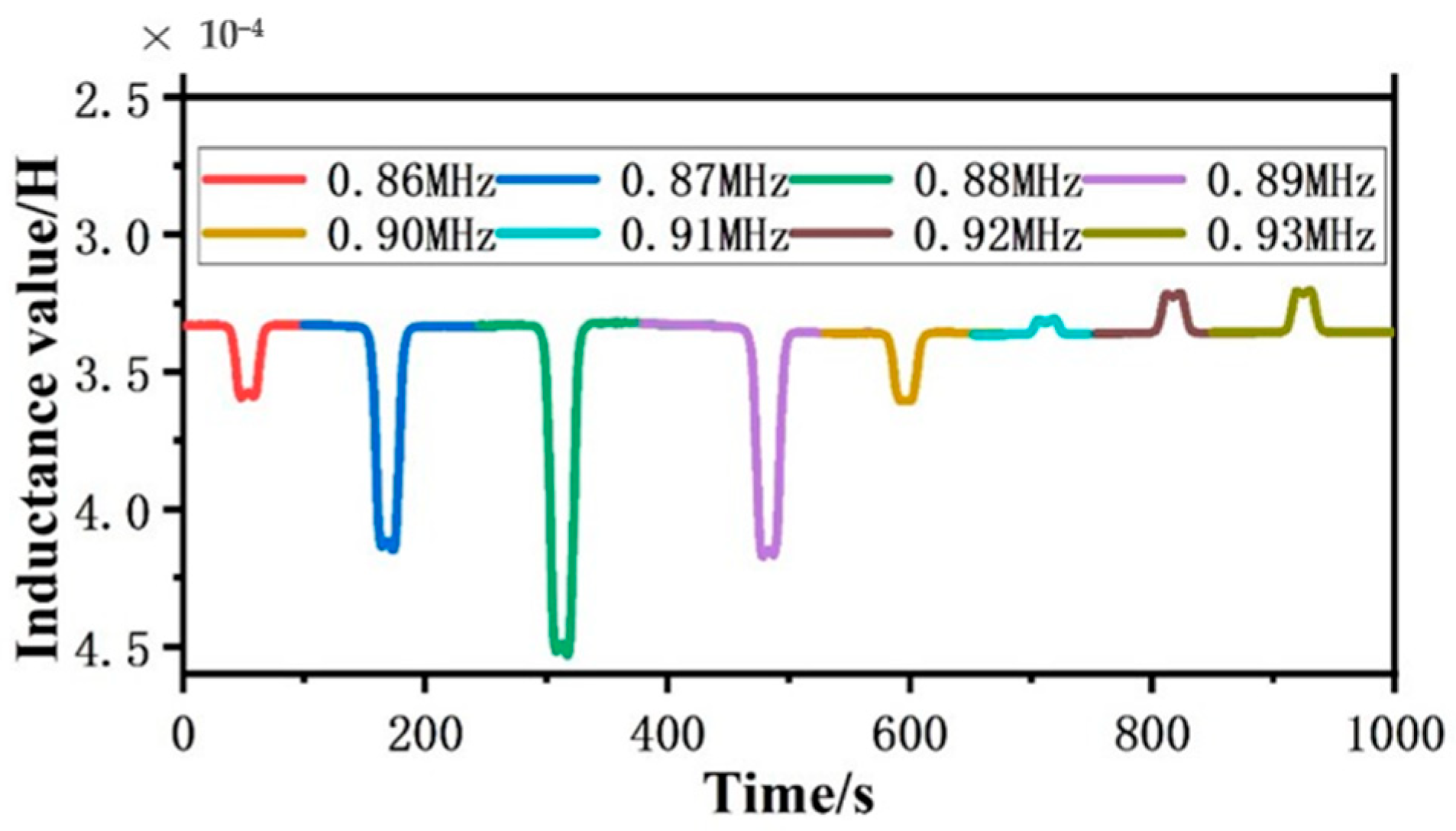
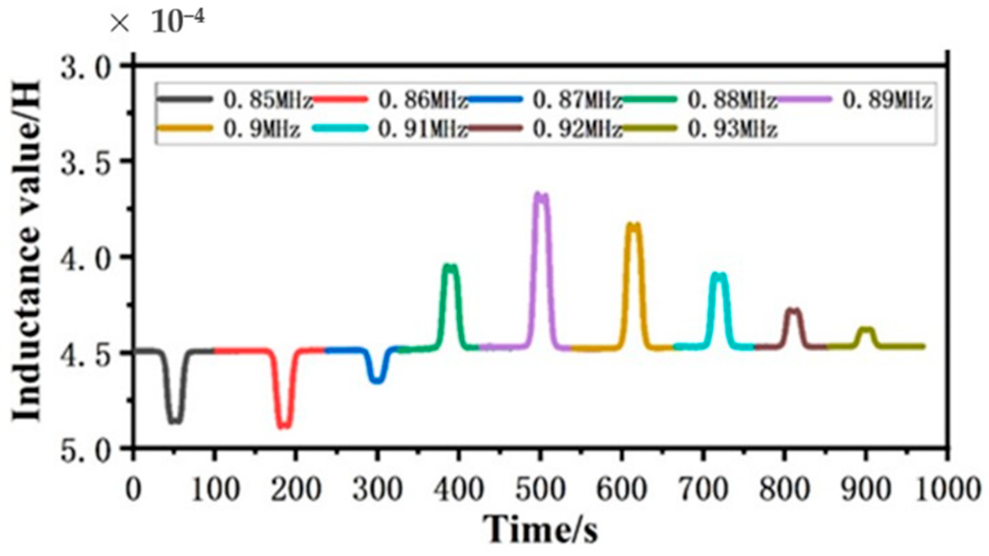
4.2. Experiment on the Selection of Optimal Excitation Frequency

In the experiment, the excitation frequency is crucial for the detection sensitivity of the sensor. First, we selected an oil sample containing 410 µm iron particles and 600 µm copper particles for testing and set the detection area in the middle of the detection coil. Then, we conducted a series of experiments in the frequency range of 0.86 MHz to 0.93 MHz using an excitation voltage of 2 V and an oil flow rate of 50 μL/min. The experimental results show that the inductance amplitudes of iron and copper particles behave differently at different frequencies. Specifically, the inductance amplitude of iron particles reaches its maximum at 0.88 MHz (Figure 7), while the inductance amplitude of copper particles reaches its peak at 0.89 MHz (Figure 8). Considering that the signal quality of the iron particles is better than that of the copper particles in the experimental process, we choose 0.89 MHz as the final experimental frequency.

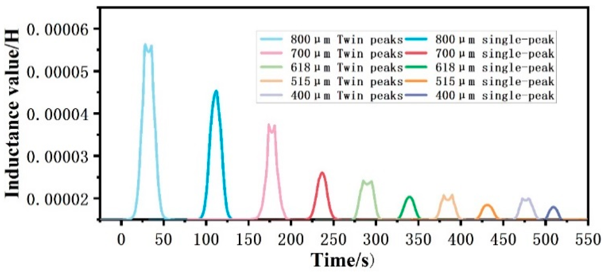
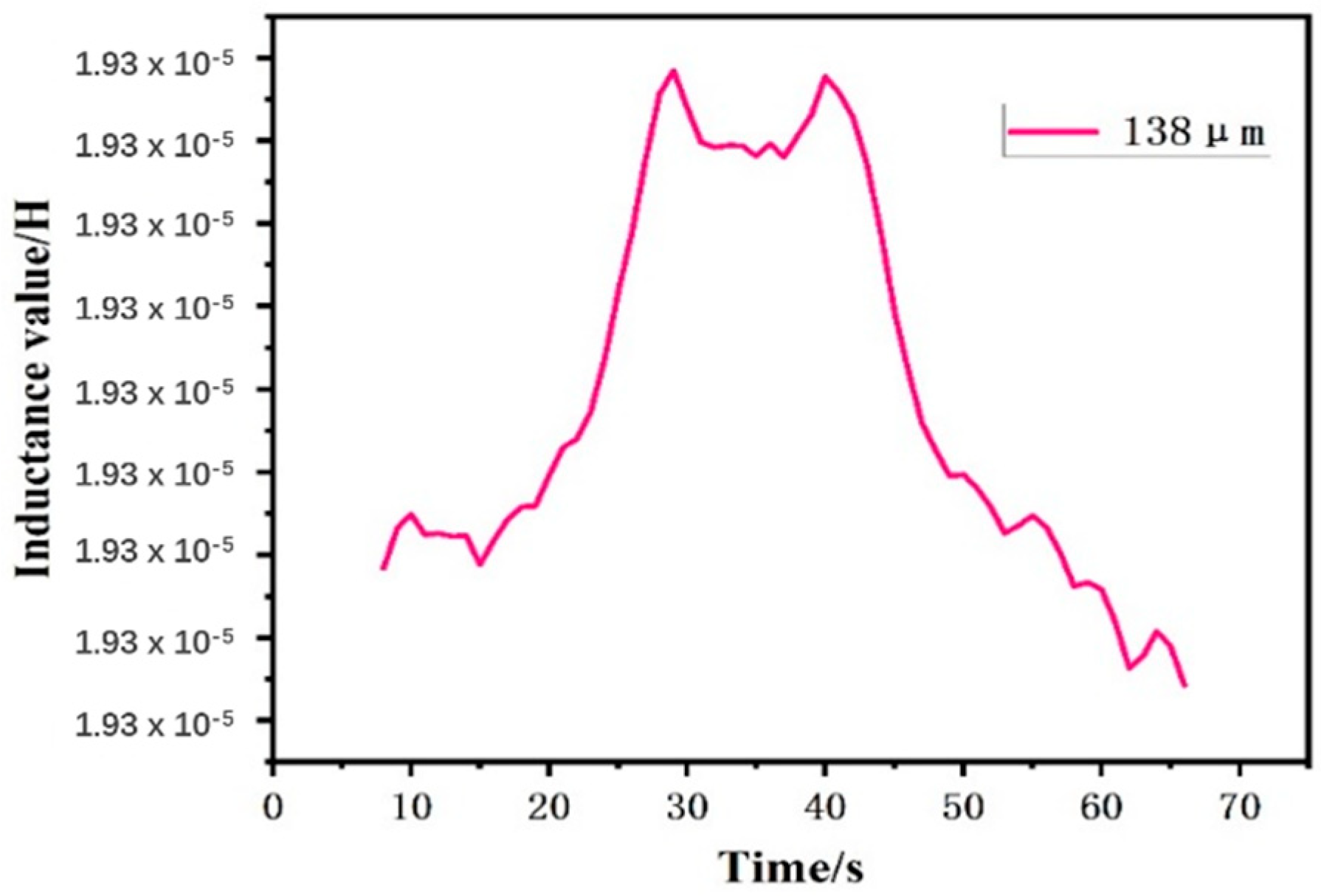
4.3. Experimental Characterization of Particle Signals under Different Detection Regions of the Sensor

In order to study the signal characteristics of wear particles of different sizes in different detection areas of the sensor, we set the excitation frequency to 0.89 MHz and the flow rate of the micro syringe pump to 50 uL/min. On this basis, we selected oil samples containing 410–800 μm iron particles and 400–800 μm copper particles. A three-dimensional coordinate system was established with the center of the coil as the origin. Path 1 is the case when the axial centerline of the microfluidic channel is the y-axis of the coordinate system. When the axial centerline of the microfluidic channel is parallel to the y-axis and the centerline passes through z = −1.5 mm, this is path 2. In the experiment, the oil samples passed through the sensor from path 1 and path 2, as shown in Figure 9. With this setup, we can compare the signal characteristics of different sized particles in different detection areas of the sensor to get a more comprehensive understanding of the nature of the wear particles and the detection effect of the sensor.

Figure 10 shows iron particles from different paths moving through the sensor detection area when the signal curves, and Figure 11 shows copper particles from different paths moving through the sensor detection area when the signal curves. It is clear from the figure that the inductance signal of the metal abrasive particles along the two paths increases with the increase in the particle size. The same particles pass through the sensor detection area at the same speed, and the inductance signal amplitude is larger and the sensitivity is higher when passing along from path 2 than when passing from path 1. Interestingly, there are two peaks in the inductive signal when passing through path 2, while there is only one peak in the inductive signal when passing through path 1. The “double-peaked” signal is significantly more recognizable and has a higher signal amplitude. The “twin peaks” signal is significantly more recognizable than the “single-peak” signal detected by conventional inductive sensors.

4.4. Pollutant Detection Experiment

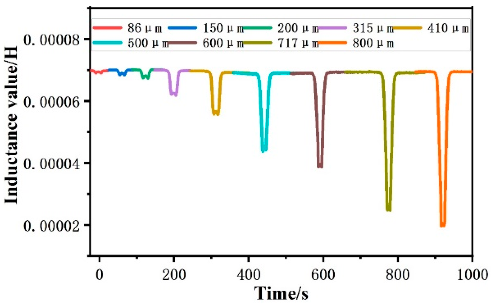
4.4.1. Ferromagnetic Metal Particle Detection Experiment

Since the signal amplitude is larger and the sensor sensitivity is higher when the particles pass through the sensor in Path 2, Path 2 was chosen as the microfluidic detection area for the subsequent experiments. When detecting iron particles, according to the particle size from large to small order for detection, the first detection was of the particle size of 800 μm iron particles, and then it gradually reduced the particle size to 86 μm, with the detected inductive signal shown in Figure 12. As shown in the picture, the amplitude of the signal is the largest for iron particles with a particle size of 800 μm, which indicates that the sensor has a significant ability to detect the large-sized particles. Figure 13 shows that the sensor detects 55 μm iron particle signal graphics, and the signal value is clearer, according to the signal fluctuation. It can be judged that there are small-size particles passing through the sensor, but the detection is not obvious.

Signal to Noise Ratio (SNR) is the ratio of received useful signal strength to received interfering signal strength [26]. In this context, the signal-to-noise ratio (SNR) serves as an indicator of the sensor’s detection capability. A higher SNR value indicates a more pronounced detection effect for pollutants. Different particle sizes result in varying signal values and SNR values. The graph demonstrates that larger wear particle sizes correspond to higher SNR values, whereas smaller particle sizes lead to lower SNR values. The sensor can detect the inductive signals of particles below 55 μm; however, the detection efficiency is relatively poor in comparison with larger wear particles.

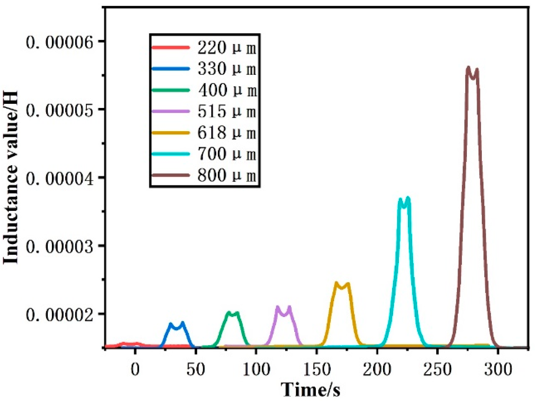
4.4.2. Non-Ferromagnetic Metal Particle Detection Experiment

The detection of copper particles still proceeded by particle size from large to small in order of detection. The first detection was of the particle size of 800 μm copper particles, followed by a gradual reduction in particle size to 220 μm, with the inductance signal detected as shown in Figure 14. It can be observed that copper particles with a particle size of 800 μm have the most obvious signal. As shown in Figure 15, for the sensor to detect the signal graph of 138 μm of copper particles, its signal amplitude is relatively small. Copper particles below 100 μm, according to the signal fluctuations, can be judged to have small particle size particles through the sensor, but due to the large error, this experiment was not considered.

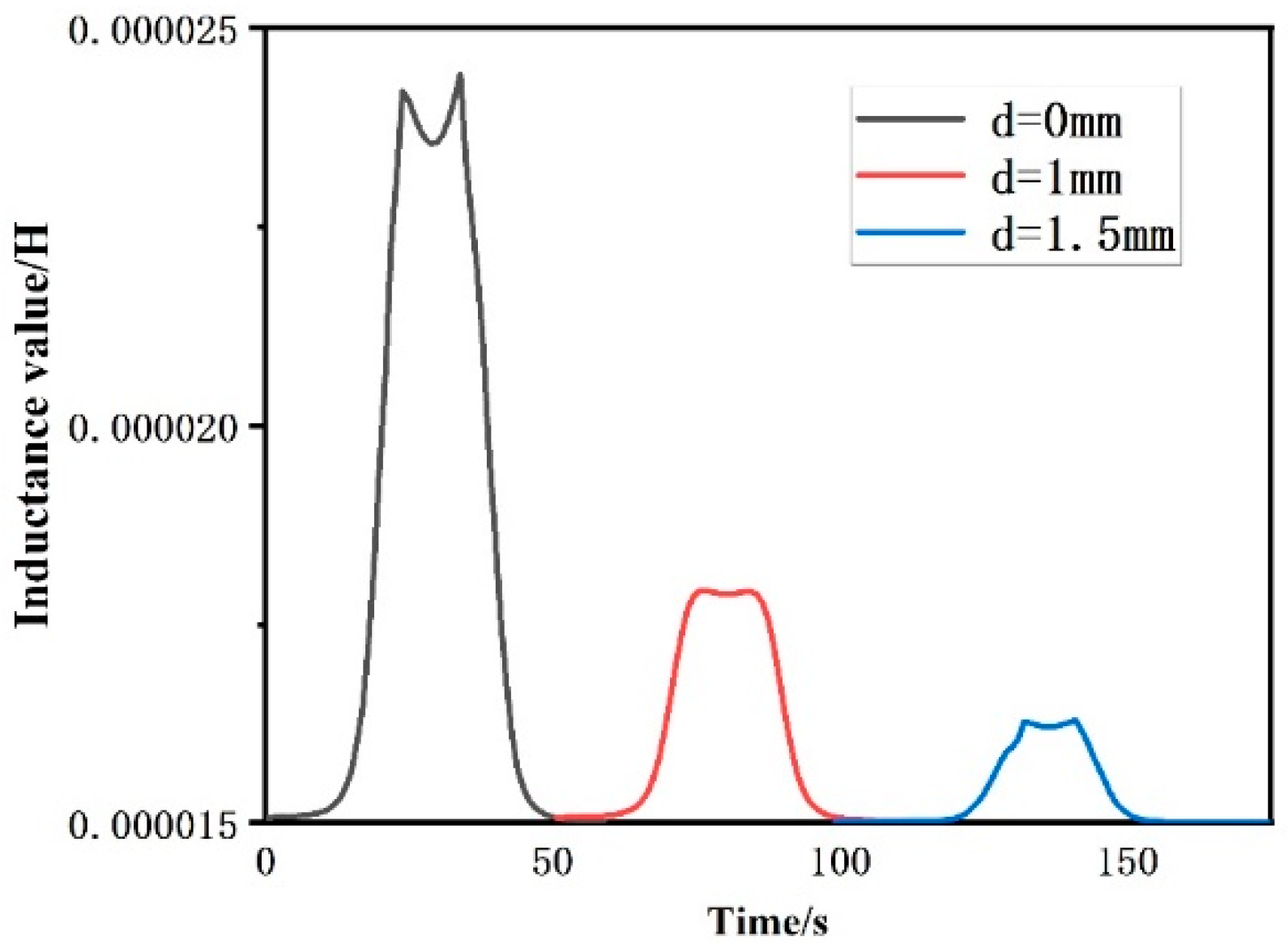
4.5. Coil Spacing Comparison Experiment

Since the sensor can perform passive detection and the LC resonance unit can be placed inside the oil pipeline in practical operation, the spacing between the detection and receiving coils is an important influencing factor in the experiment. In this experiment, oil samples containing 410 μm iron particles and 618 μm copper particles are selected, and the selected oil samples are passed through the detection area of the sensor with different coil spacing structures to measure their inductive signal values. The sensor structures with different coil distances are shown in Figure 16. Figure 16a shows the sensor structure when d = 0 mm, i.e., two coils are close together; Figure 16b shows the sensor structure when d = 1 mm; and Figure 16c shows the sensor structure when d = 1.5 mm.

The detection results are shown in Figure 17 and Figure 18. The experimental results show that the further the distance between the detecting coil and the receiving coil, the lower the amplitude of the inductive signal from the wear particles; when the two coils are close to each other, the sensor has the highest sensitivity, and the amplitude of the inductive signal is the largest; when there is a certain distance between the two coils, the amplitude of the inductive signal starts to decrease, but different particles signals can still be recognized, which makes it possible to achieve the wireless transmission of the wear particle signals from a long distance.

5. Conclusions

The purpose of this study is to explore an inductive oil detection sensor for detecting metal abrasive debris in oil and its wireless signal transmission circuit. First, we used COMSOL software to simulate the magnetic field distribution of the sensor structure and the signal characteristics of the particulate contaminants as they pass through the oil detection sensor. Subsequently, through a series of experiments, we determined the optimal excitation frequency of the oil detection sensor and the optimal spacing of the two coils, and we explored the inductive signal characteristics of the metal abrasive chips under different detection areas. The results show that the highest sensitivity is achieved when the microfluidic channel is set in the middle of the detection coils, and a “double-peak” inductance signal can be detected, which provides the basis for portable detection. The sensor’s simple structure, obvious signal characteristics, and high detection sensitivity are well suited for the detection of metal abrasives in hydraulic fluids. This study provides an idea for realizing the wireless detection of the oil detection sensor.

References

1. Zhang, Z.; Hu, S.; Bai, C.; Wang, C.; Li, H.; Zhang, H. Characterization of multi-abrasive mixed signals from LC resonance-based dual-coil oil detection sensors. IEEE Sens. J. 2024. [Google Scholar] [CrossRef]
2. Huang, H.; He, S.; Xie, X. Research on the influence of inductive wear particle sensor coils on debris detection. AIP Adv. 2022, 12, 075204. [Google Scholar] [CrossRef]
3. Liu, Z.; Liu, Y.; Zuo, H. An oil wear particles inline optical sensor based on motion characteristics for rotating machines condition monitoring. Machines 2022, 10, 727. [Google Scholar] [CrossRef]
4. Liu, Z.; Liu, Y.; Zuo, H. Oil debris and viscosity monitoring using optical measurement based on Response Surface Methodology. Measurement 2022, 195, 111152. [Google Scholar] [CrossRef]
5. Bastidas, S.; Allmaier, H. Application of a Wear Debris Detection System to Investigate Wear Phenomena during Running-In of a Gasoline Engine. Lubricants 2023, 11, 237. [Google Scholar] [CrossRef]
6. Dang, Z.; Jiang, Y.; Su, X.; Wang, Z.; Wang, Y.; Sun, Z.; Zhao, Z.; Zhang, C.; Hong, Y.; Liu, Z. Particle Counting Methods Based on Microfluidic Devices. Micromachines 2023, 14, 1722. [Google Scholar] [CrossRef]
7. Bai, C.; Zhang, H.; Zeng, L. High-Throughput Sensor to Detect Hydraulic Oil Contamination Based on Microfluidics. IEEE Sens. J. 2019, 19, 8590–8596. [Google Scholar] [CrossRef]
8. Weser, R.; Wöckel, S.; Hempel, U. Particle characterization in highly concentrated suspensions by ultrasound scattering method. Sens. Actuators A Phys. 2013, 202, 30–36. [Google Scholar] [CrossRef]
9. Du, L.; Zhe, J. An integrated ultrasonic–inductive pulse sensor for wear debris detection. Smart Mater. Struct. 2012, 22, 025003. [Google Scholar] [CrossRef]
10. Iwai, Y.; Honda, T.; Miyajima, T. Quantitative estimation of wear amounts by real time measurement of wear debris in lubricating oil. Tribol. Int. 2010, 43, 388–394. [Google Scholar] [CrossRef]
11. Zeng, X. A high sensitive multi-parameter micro sensor for the detection of multi-contamination in hydraulic oil. Sens. Actuators A. Phys. 2018, 282, 197–205. [Google Scholar] [CrossRef]
12. Han, Z.; Wang, Y.; Qing, X. Characteristics study of in-situ capacitive sensor for monitoring lubrication oil debris. Sensors 2017, 17, 2851. [Google Scholar] [CrossRef] [PubMed]
13. Raadnui, S.; Kleesuwan, S. Low-cost condition monitoring sensor for used oil analysis. Wear 2005, 259, 1502–1506. [Google Scholar] [CrossRef]
14. Du, L.; Zhe, J. Parallel sensing of metallic wear debris in lubricants using under sampling data processing. Tribol. Int. 2012, 53, 28–34. [Google Scholar] [CrossRef]
15. Xiao, H.; Wang, X.; Li, H. An inductive debris sensor for a large-diameter lubricating oil circuit based on a high-gradient magnetic field. Appl. Sci. 2019, 9, 1546. [Google Scholar] [CrossRef]
16. Sun, J.; Wang, L.; Li, J. Online oil debris monitoring of rotating machinery: A detailed review of more than three decades. Mech. Syst. Signal Process. 2021, 149, 107341. [Google Scholar] [CrossRef]
17. Zhang, Y.; Hong, J.; Shi, H. Magnetic plug sensor with bridge nonlinear correction circuit for oil condition monitoring of marine machinery. J. Mar. Sci. Eng. 2022, 10, 1883. [Google Scholar] [CrossRef]
18. Yu, B.; Cao, N.; Zhang, T. A novel signature extracting approach for inductive oil debris sensors based on simplistic geometry mode decomposition. Measurement 2021, 185, 110056. [Google Scholar] [CrossRef]
19. Shen, X.; Han, Q.; Wang, Y. Research on Detection Performance of Four-Coil Inductive Debris Sensor. IEEE Sens. J. 2023, 23, 6717–6727. [Google Scholar] [CrossRef]
20. Qian, M.; Ren, Y.; Feng, Z. Wear Debris Sensor Using Intermittent Excitation for High Sensitivity, Wide Detectable Size Range, and Low Heat Generation. IEEE Trans. Ind. Electron. 2022, 70, 6386–6394. [Google Scholar] [CrossRef]
21. Zhu, X.; Du, L.; Zhe, J. A 3 × 3 wear debris sensor array for real time lubricant oil conditioning monitoring using synchronized sampling. Mech. Syst. Signal Process. 2017, 83, 296–304. [Google Scholar] [CrossRef]
22. Xie, Y.C.; Shi, H.T.; Zhang, H.P. A bridge-type inductance sensor with a two-stage filter circuit for high-precision detection of metal debris in the oil. IEEE Sens. J. 2021, 21, 17738–17748. [Google Scholar] [CrossRef]
23. Feng, S.; Tan, J.; Wen, Y. Sensing model for detecting ferromagnetic debris based on a high-gradient magnetostatic field. IEEE/ASME Trans. Mechatron. 2021, 27, 2440–2449. [Google Scholar] [CrossRef]
24. Zhao, K.; Wei, Y.; Zhao, P. Tunable magnetophoretic method for distinguishing and separating wear debris particles in a Fe-PDMS based microfluidic chip. Electrophoresis 2023, 44, 1210–1219. [Google Scholar] [CrossRef]
25. Available online: https://baike.baidu.com/item/SINR (accessed on 15 January 2024).
26. Zhang, H.P.; Zhang, Z.; Zhao, X.P.; Li, H.; Li, W.; Wang, C.Y.; Bai, C.Z.; Hu, S.K. An LC resonance-based sensor for multi-contaminant detection in oil fluids. IEEE Sens. J. 2024, 24, 9772–9782. [Google Scholar] [CrossRef]
Figure 1. Sensor structure diagram.
Jmse 12 01704 g001
Figure 2. Circuit model.
Jmse 12 01704 g002
Figure 3. 3D view of the model of the sensor in COMSOL software.
Jmse 12 01704 g003
Figure 4. Three-dimensional plot of magnetic flux density when the sensor is at resonant frequency. Detecting the flux density mode of a coil cross-section.
Jmse 12 01704 g004
Figure 5. Detecting the flux density mode of a coil cross-section.
Jmse 12 01704 g005
Figure 6. Diagram of sensor-built detection system.
Jmse 12 01704 g006
Figure 7. Signal profile of 410 µm iron particles at different excitation frequencies.
Jmse 12 01704 g007
Figure 8. Signal profile of 600 µm copper particles at different excitation frequencies.
Jmse 12 01704 g008
Figure 9. Comparison of different paths of microfluidic channel: (a) Path 1; (b) Path 2.
Jmse 12 01704 g009
Figure 10. Signal curve for 410–800 μm Iron particles.
Jmse 12 01704 g010
Figure 11. Signal curve for 400–800 μm copper particles.
Jmse 12 01704 g011
Figure 12. 86–800 μm iron particles’ signal curve.
Jmse 12 01704 g012
Figure 13. Signal curve for detection of 55 μm iron particles.
Jmse 12 01704 g013
Figure 14. 220–800 μm copper particles’ signal curve.
Jmse 12 01704 g014
Figure 15. Signal curve for detection of 138 μm copper particles.
Jmse 12 01704 g015
Figure 16. Comparison of different coil spacing models: (a) Coil spacing d = 0 mm; (b) Coil spacing d = 1 mm; (c) Coil spacing d = 1.5 mm.
Jmse 12 01704 g016
Figure 17. Inductance signal curves of 410 μm iron particles under different sensor configurations.
Jmse 12 01704 g017
Figure 18. Inductance signal curves of 618 μm copper particles under different sensor configurations.
Jmse 12 01704 g018