Small-Scale Biophysical Interactions and Dinophysis Blooms: Case Study in a Strongly Stratified Chilean Fjord

 ,
,  , ,
, ,  , , ,
, , ,
Abstract
:1. Introduction
2. Materials and Methods
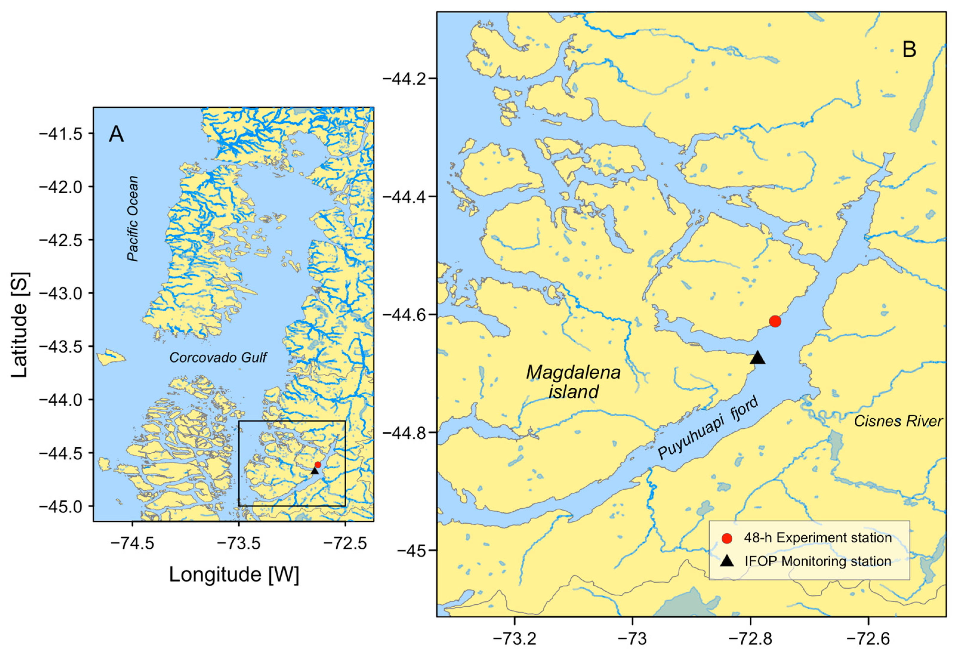
2.1. Study Area
2.2. IFOP Monitoring Program
2.3. Field Cruise Sampling
2.3.1. Hydrography and Turbulence Measurements
2.3.2. Phytoplankton and Physiological Conditions
2.4. Sample Analyses
2.4.1. Microphytoplankton Analysis
2.4.2. Division Rates Estimation of Dinophysis Cells
2.4.3. Toxins Sample Extraction
2.4.4. Toxin Detection and Quantification
2.5. Statistical Analysis
3. Results
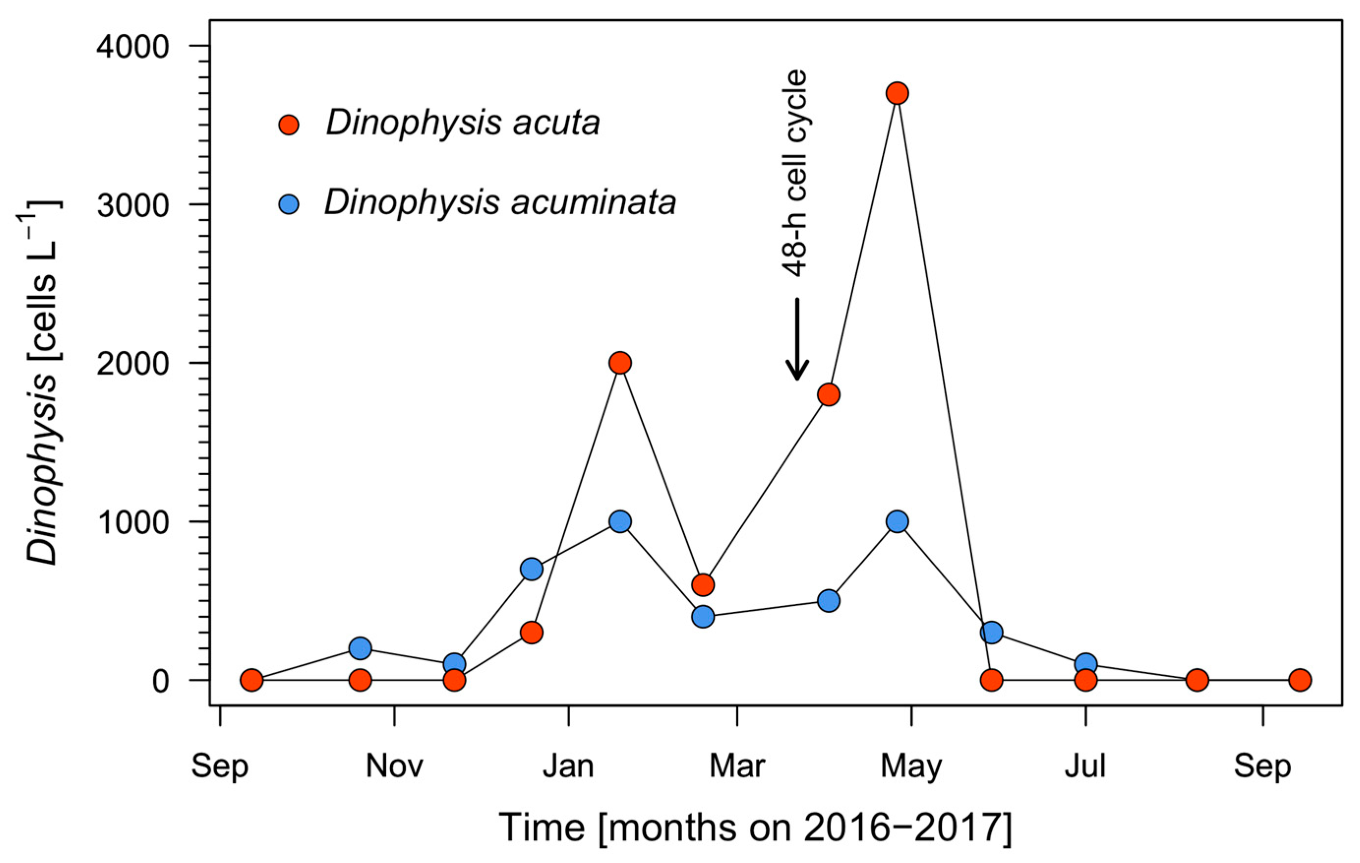
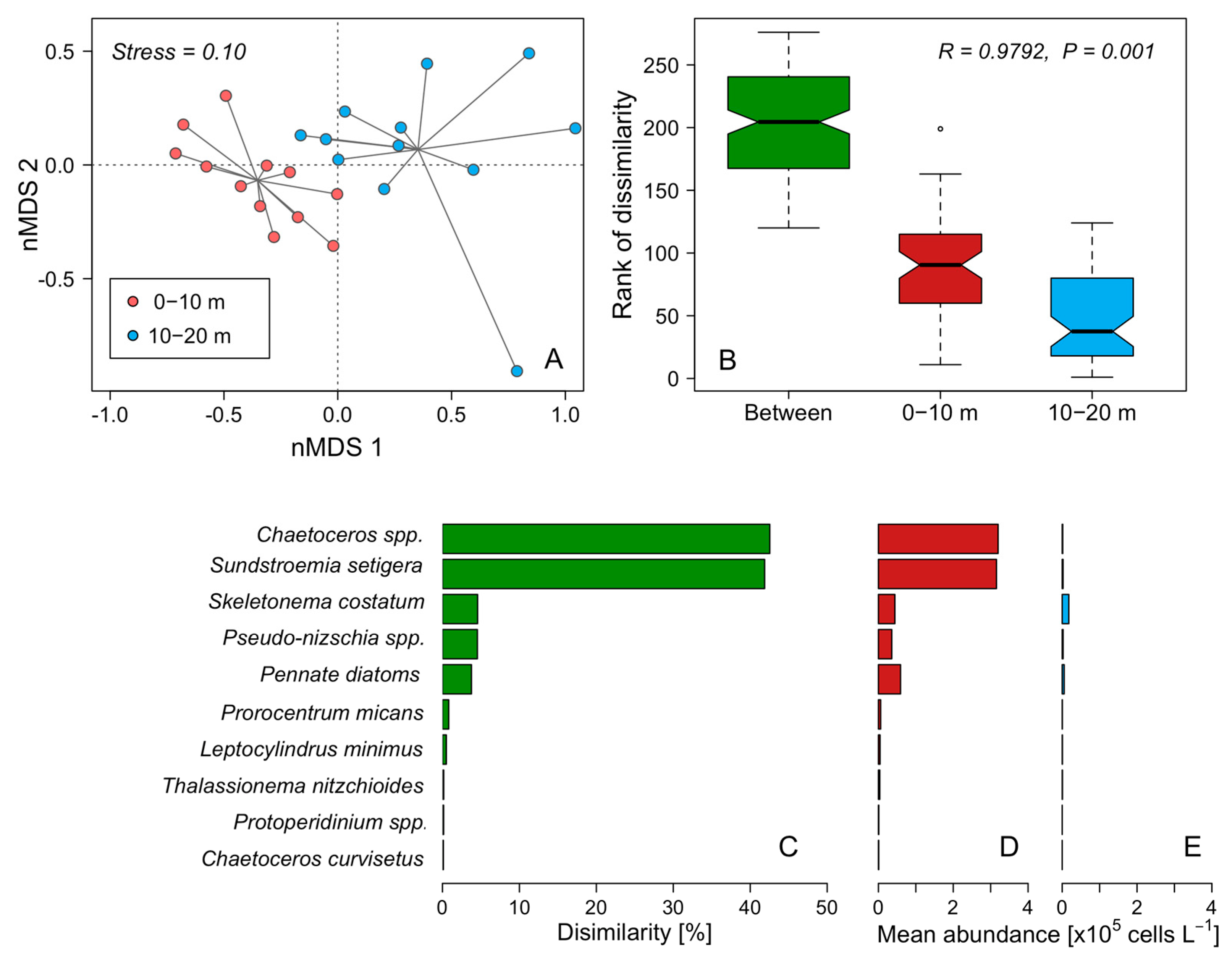
3.1. Seasonal Changes in Hydrographic Conditions and Dinophysis Populations in 2016–2017
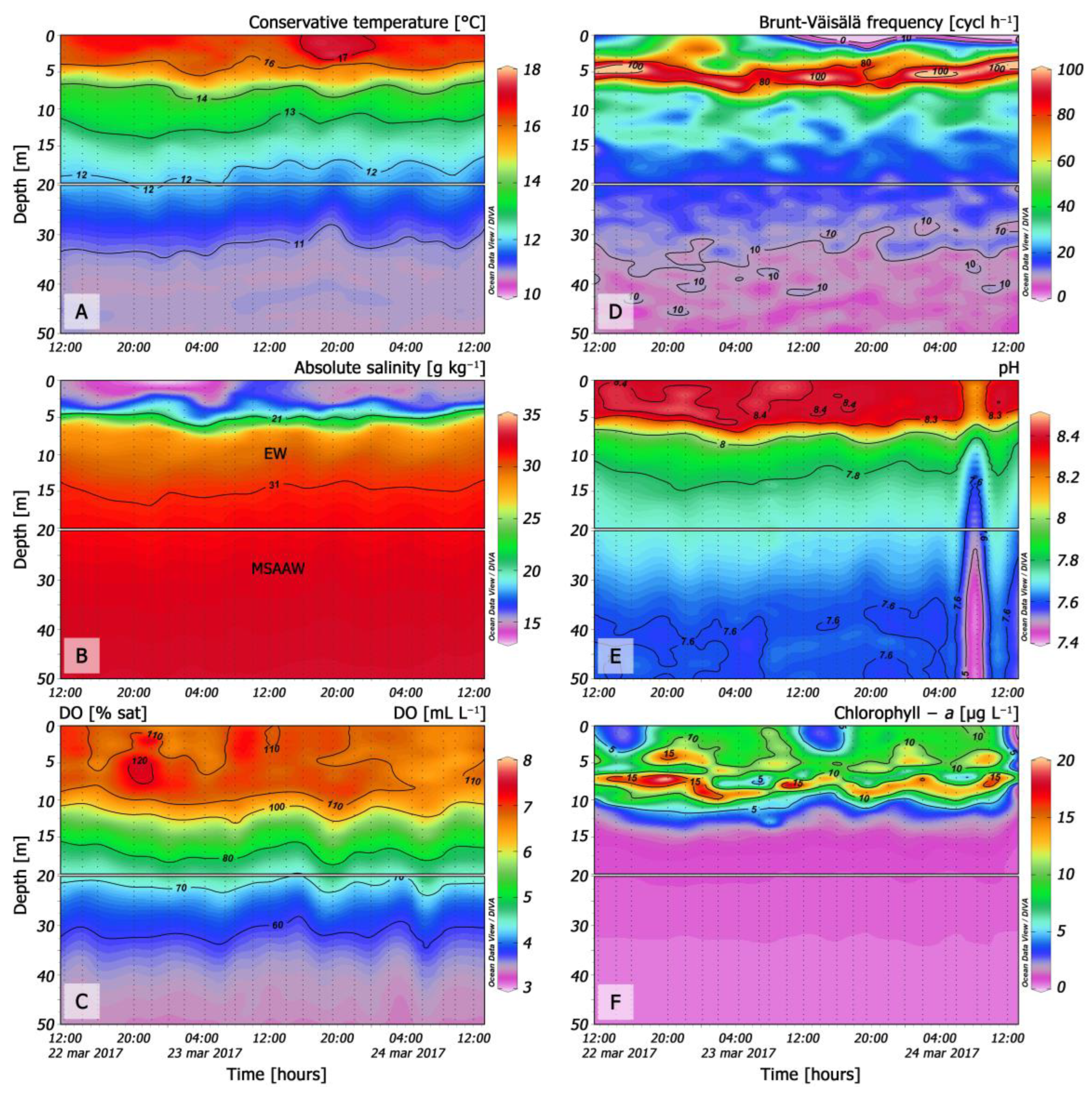
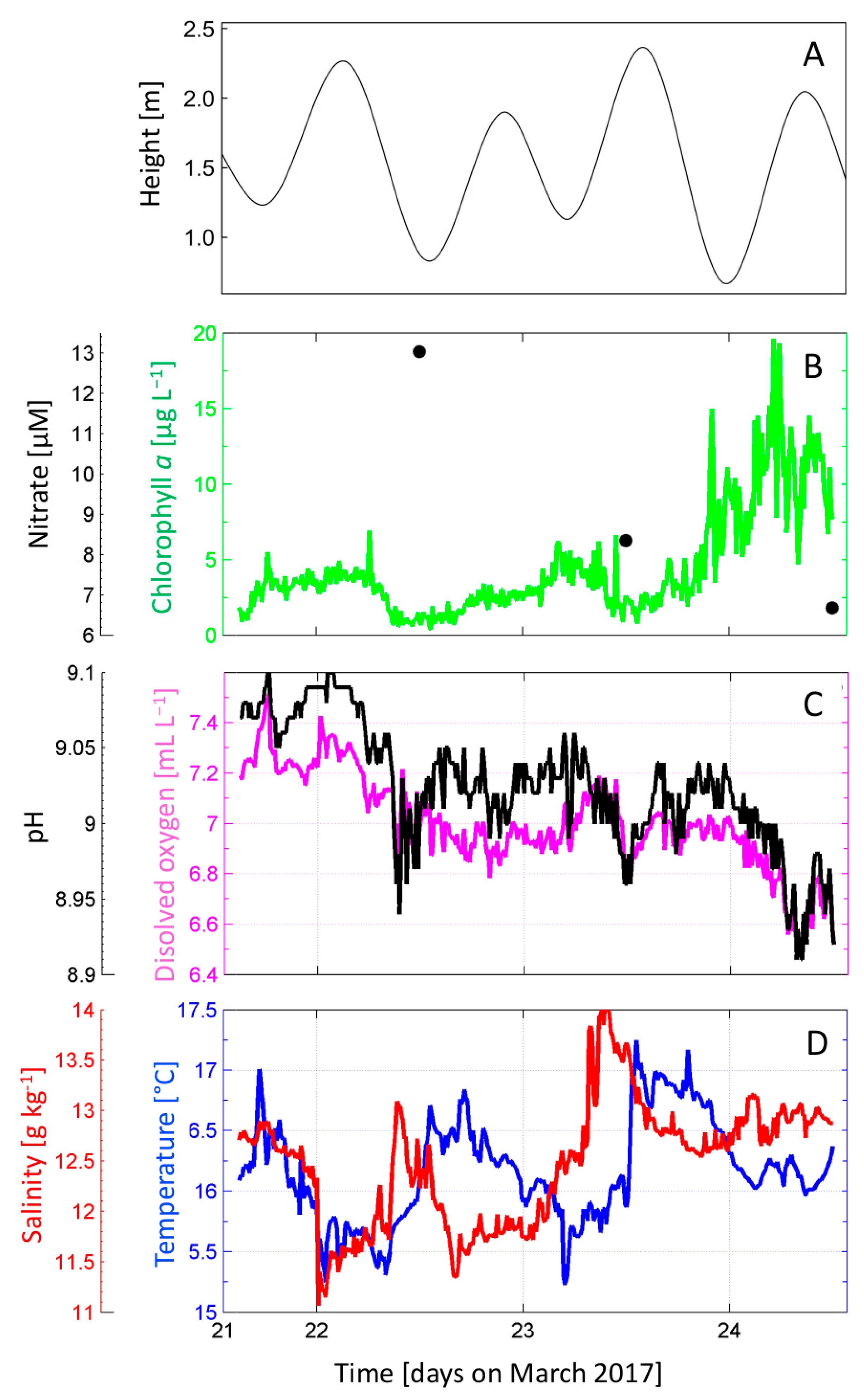
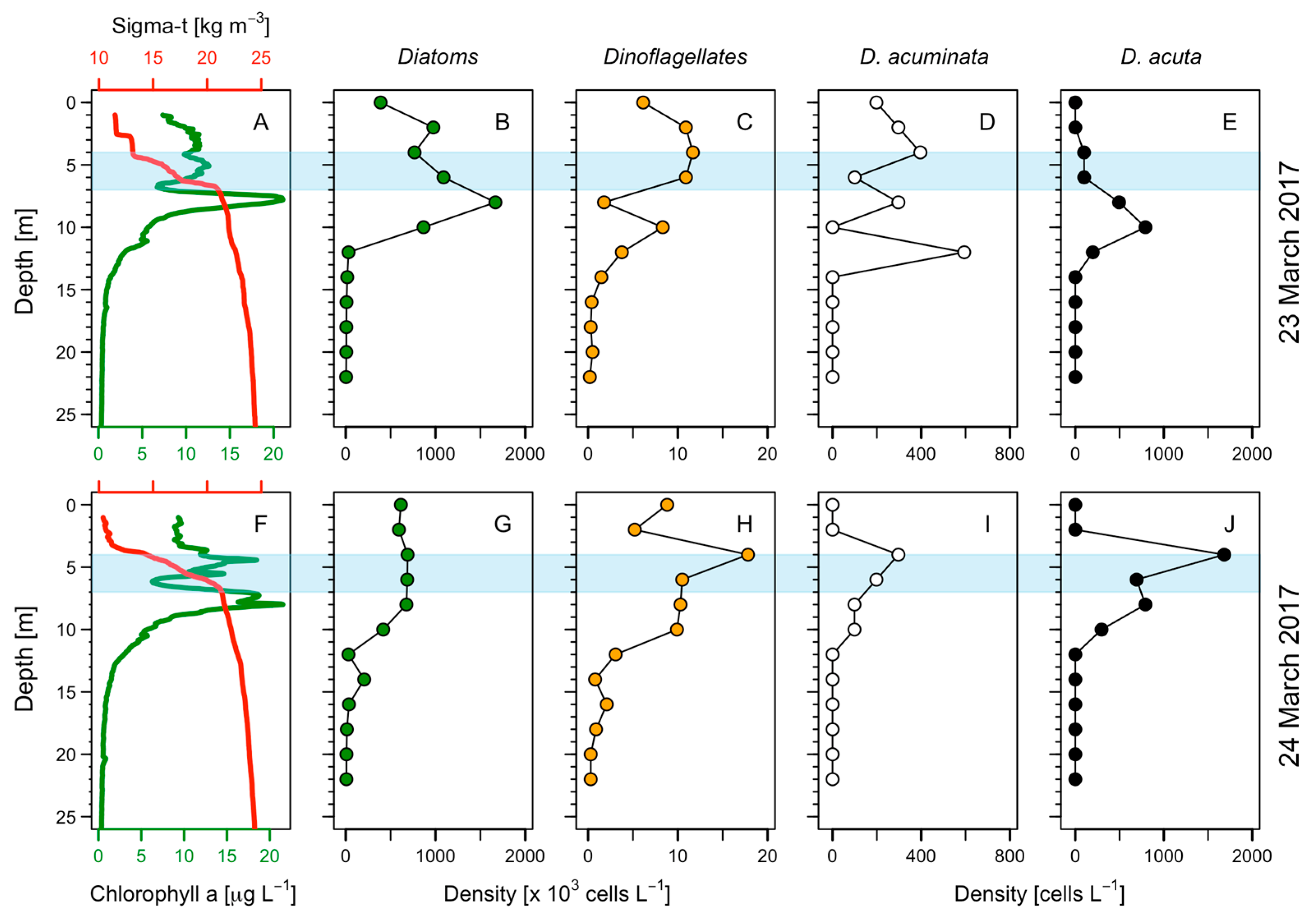
3.2. Hydrography, Chlorophyll-a, and Nutrients during the 48 h Study
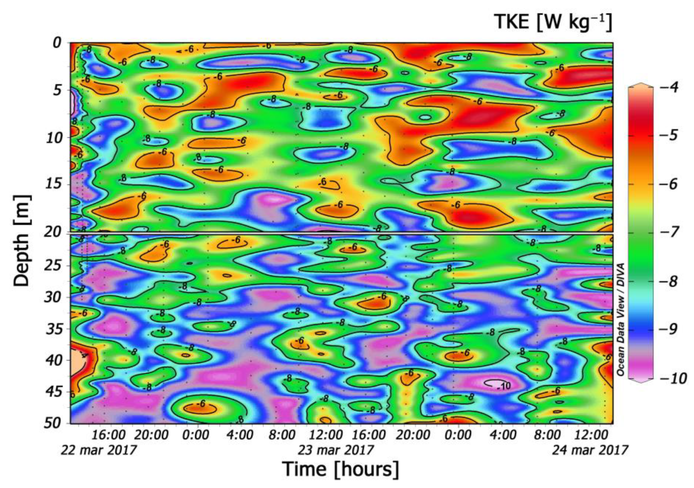
3.3. Turbulence
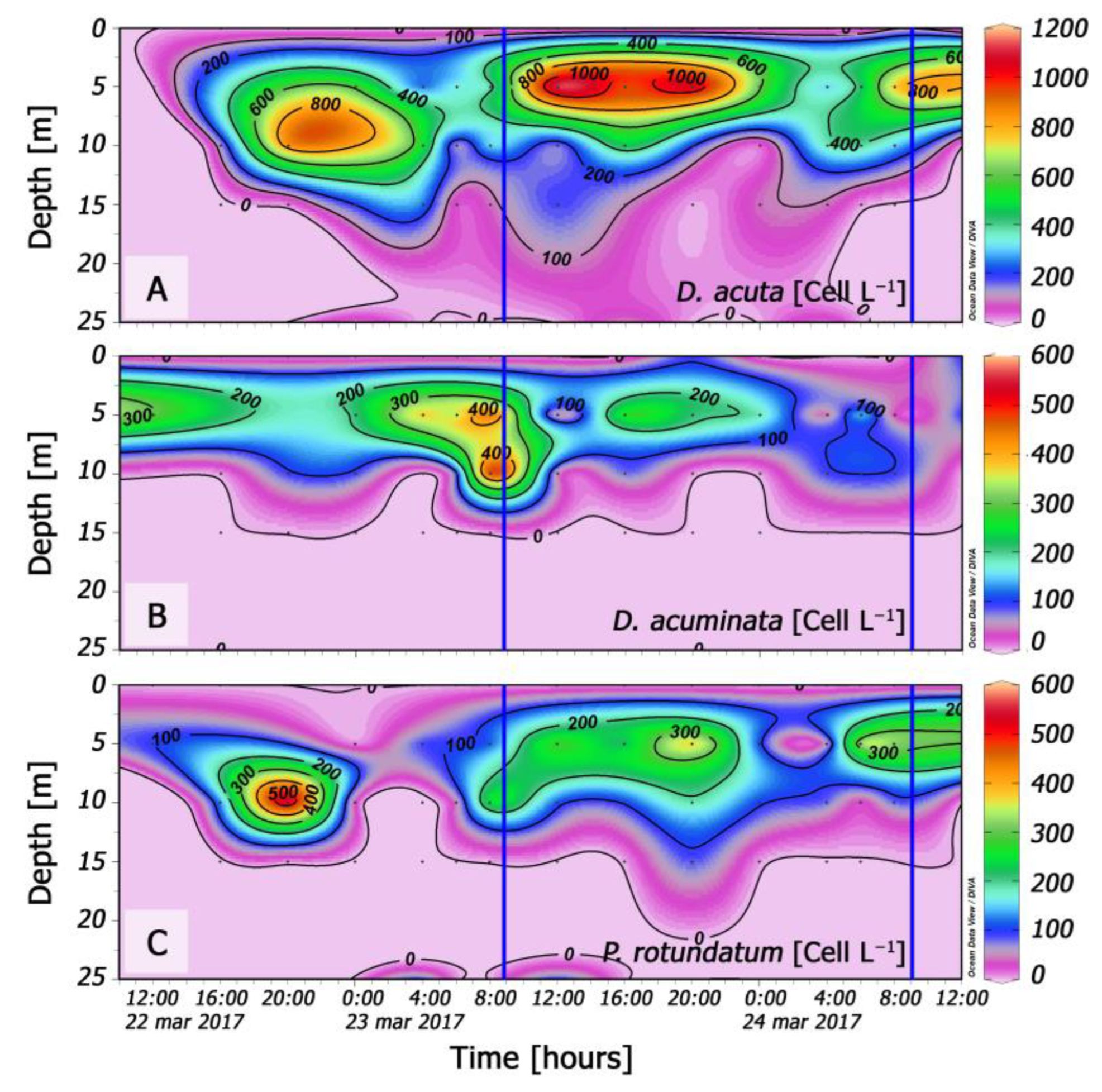
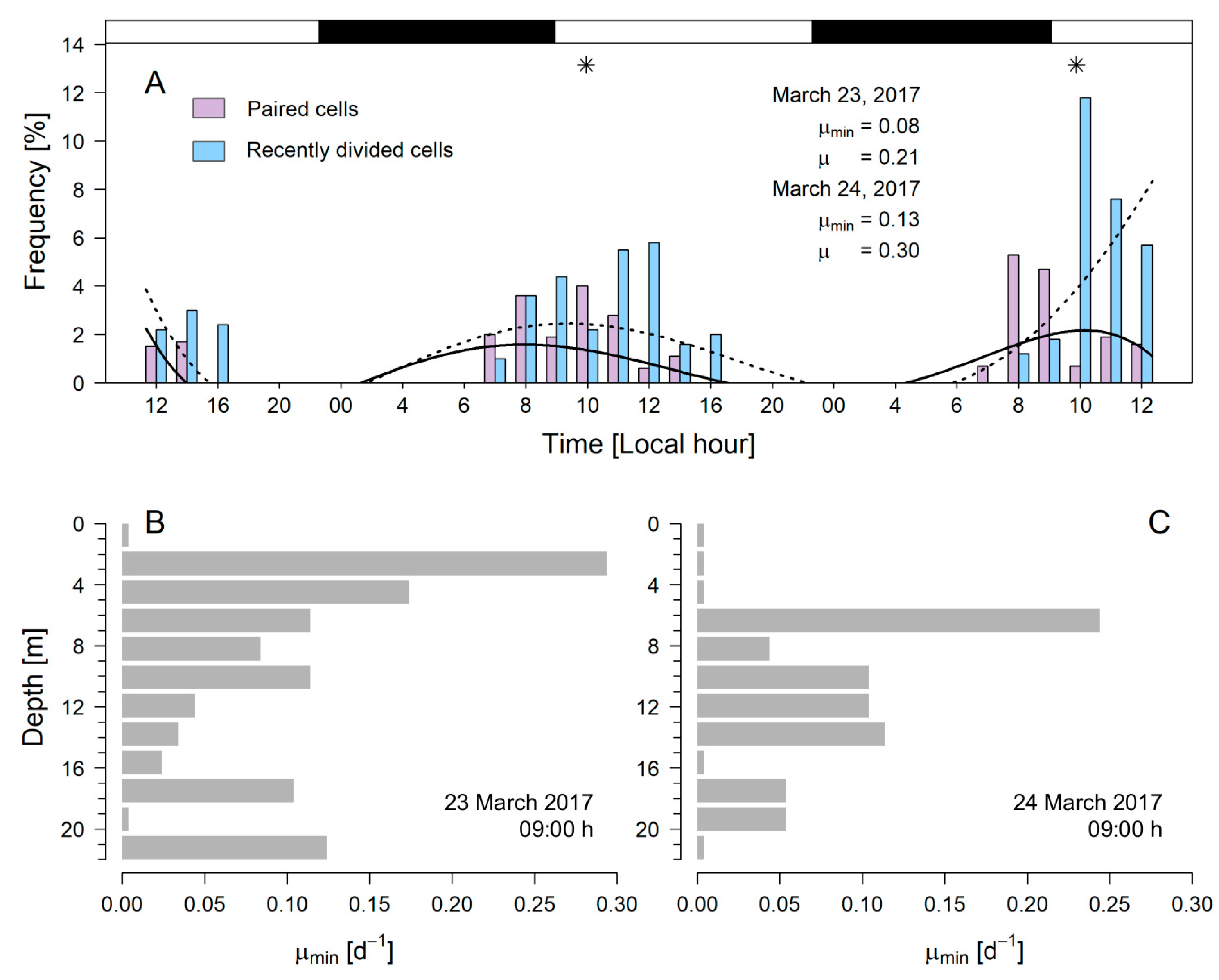
3.4. Distribution of Dinophysis during the 48 h Cycle
3.5. Estimates of µ during the 48 h Study
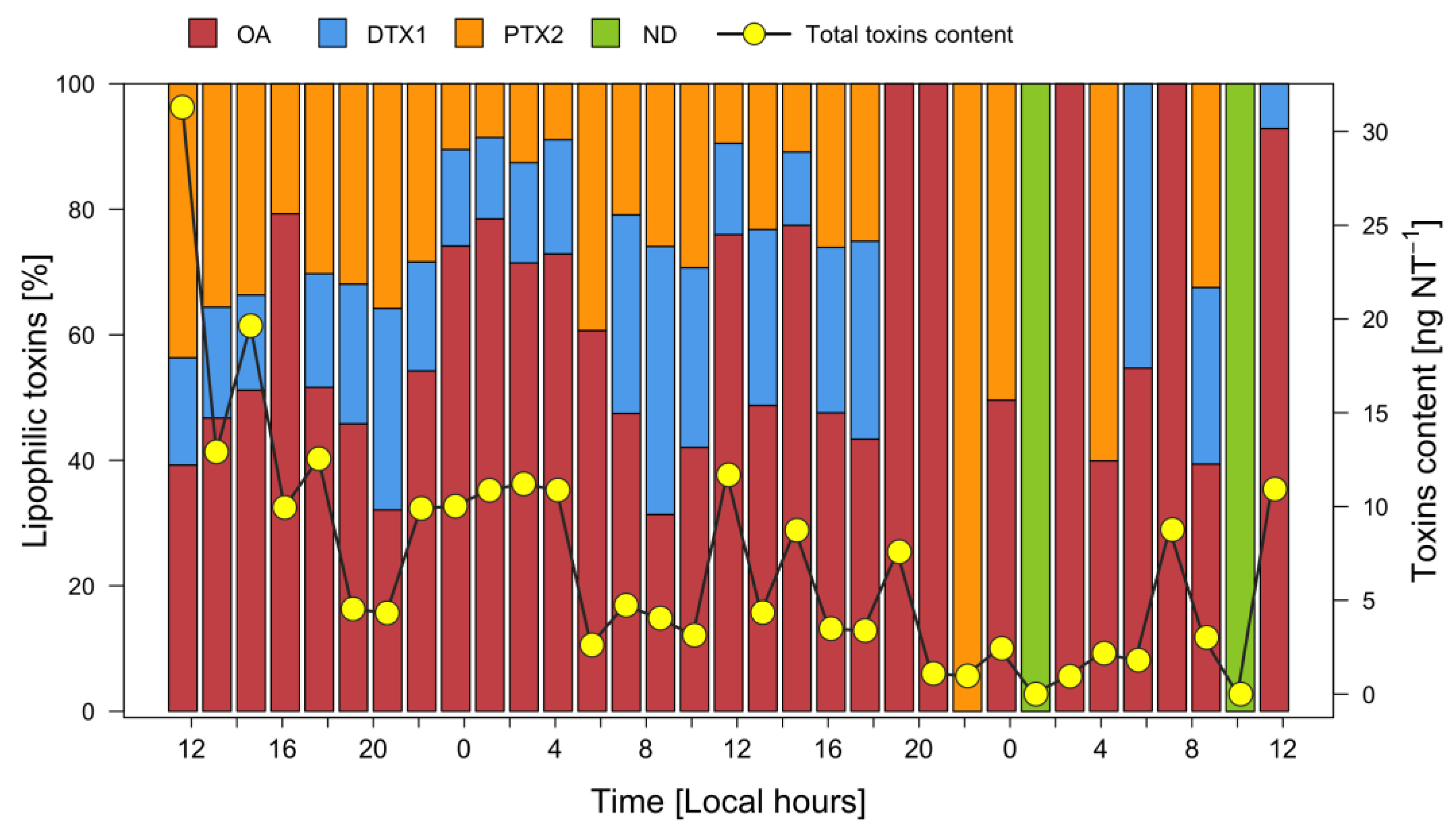
3.6. Lipophilic Toxins in Plankton
4. Discussion
4.1. Hydrography and Phytoplankton Distribution in the Study Year
4.2. Vertical Gradients, Segregation of Diatoms and Dinoflagellates Cell Maxima, and Thin-Layer Formation during the 48 h Study
4.3. In Situ Division Rates of Dinophysis acuta and Toxins
5. Conclusions
Author Contributions
Funding
Institutional Review Board Statement
Informed Consent Statement
Data Availability Statement
Acknowledgments
Conflicts of Interest
Appendix A

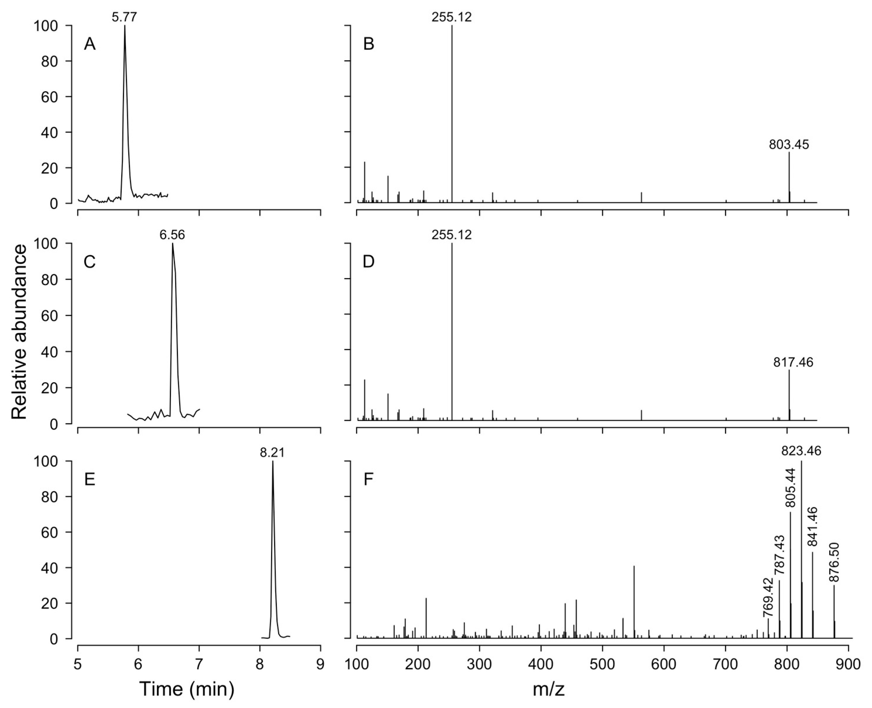
| Compound | Abbreviation | Chemical Formula | Molecular Ion | m/z Calculated | CE |
|---|---|---|---|---|---|
| Okadaic acid | OA | C44H68O13 | [M-H]− | 803.4587 | 55 |
| Dinophysistoxin-1 | DTX-1 | C45H70O13 | [M-H]− | 817.4744 | 55 |
| Dinophysistoxin-2 | DTX-2 | C44H68O13 | [M-H]− | 803.4587 | 55 |
| Yessotoxin | YTX | C55H82O21S2 | [M-2H]2− | 570.2322 | 34 |
| homo-Yessotoxin | homoYTX | C56H84O21S2 | [M-2H]2− | 577.2401 | 34 |
| Azaspiracid-1 | AZA-1 | C47H71NO12 | [M + H]+ | 842.5049 | 34 |
| Azaspiracid-2 | AZA-2 | C48H73NO12 | [M + H]+ | 856.5206 | 34 |
| Azaspiracid-3 | AZA-3 | C46H69NO12 | [M + H]+ | 828.4893 | 40 |
| Gymnodimine | GYM | C32H45NO7 | [M + H]+ | 508.3421 | 34 |
| Pinnatoxin-G | PnTX | C42H63NO7 | [M + H]+ | 694.4677 | 50 |
| 13-desMe-SPX C | SPX-1 | C42H61NO7 | [M + H]+ | 692.4521 | 30 |
| Pectenotoxin-2 | PTX2 | C47H70O14 | [M + NH4]+ | 876.5104 | 30 |
References
- Wells, M.L.; Trainer, V.L.; Smayda, T.J.; Karlson, B.S.; Trick, C.G.; Kudela, R.M.; Ishikawa, A.; Bernard, S.; Wulff, A.; Anderson, D.M.; et al. Harmful algal blooms and climate change: Learning from the past and present to forecast the future. Harmful Algae 2015, 49, 68–93. [Google Scholar] [CrossRef] [PubMed]
- Davidson, K.; Jardine, S.L.; Martino, S.; Myre, G.B.; Peck, L.E.; Raymond, R.N.; West, J.J. The economic impacts of harmful algal blooms on salmon cage aquaculture. In GlobalHAB: Evaluating, Reducing and Mitigating the Cost of Harmful Algal Blooms: A Compendium of Case Studies; Trainer, V.L., Ed.; PICES Scientific Report: Livingston, UK, 2020; Volume 59, pp. 84–94. [Google Scholar]
- Hallegraeff, G.M.; Aligizaki, K.; Amzil, Z.; Anderson, P.; Anderson, D.M.; Arneborg, L. Global HAB Status Report. A Scienfic Summary for Policy Makers; Hallegraeff, G.M., Enevoldsen, H., Zingone, A., Eds.; IOC Informa on Document, 1399; UNESCO: Paris, France, 2021. [Google Scholar]
- Díaz, P.A.; Álvarez, A.; Varela, D.; Pérez-Santos, I.; Díaz, M.; Molinet, C.; Seguel, M.; Aguilera-Belmonte, A.; Guzmán, L.; Uribe, E.; et al. Impacts of harmful algal blooms on the aquaculture industry: Chile as a case study. Perspect. Phycol. 2019, 6, 39–50. [Google Scholar] [CrossRef]
- Lembeye, G.; Yasumoto, T.; Zhao, J.; Fernández, R. DSP outbreak in Chilean fjords. In Toxic Phytoplankton Blooms in the Sea; Smayda, T.J., Shimizu, Y., Eds.; Elsevier: Amsterdam, The Netherlands, 1993; pp. 525–529. [Google Scholar]
- Alves de Souza, C.; Varela, D.; Contreras, C.; de la Iglesia, P.; Fernández, P.; Hipp, B.; Hernández, C.; Riobó, P.; Reguera, B.; Franco, J.M.; et al. Seasonal variability of Dinophysis spp. and Protoceratium reticulatum associated to lipophilic shellfish toxins in a strongly stratified Chilean fjord. Deep Sea Res. II 2014, 101, 152–162. [Google Scholar] [CrossRef]
- Díaz, P.A.; Álvarez, G.; Pizarro, G.; Blanco, J.; Reguera, B. Lipophilic toxins in Chile: History, producers and impacts. Mar. Drugs 2022, 20, 122. [Google Scholar] [CrossRef]
- Sernapesca. Anuario Estadistico de Pesca; Servicio Nacional de Pesca: Valparaíso, Chile, 2022. [Google Scholar]
- Reguera, B.; Riobó, P.; Rodríguez, F.; Díaz, P.A.; Pizarro, G.; Paz, B.; Franco, J.M.; Blanco, J. Dinophysis toxins: Causative organisms, distribution and fate in shellfish. Mar. Drugs 2014, 12, 394–461. [Google Scholar] [CrossRef]
- Díaz, P.; Molinet, C.; Cáceres, M.; Valle-Levinson, A. Seasonal and intratidal distribution of Dinophysis spp in a Chilean fjord. Harmful Algae 2011, 10, 155–164. [Google Scholar] [CrossRef]
- Baldrich, A.; Pérez-Santos, I.; Álvarez, G.; Reguera, B.; Fernández-Pena, C.; Rodríguez-Villegas, C.; Araya, M.; Álvarez, F.; Barrera, F.; Karasiewicz, S.; et al. Niche differentiation of Dinophysis acuta and D. acuminata in a stratified fjord. Harmful Algae 2021, 103, 102010. [Google Scholar] [CrossRef]
- Díaz, P.A.; Pérez-Santos, I.; Álvarez, G.; Garreaud, R.; Pinilla, E.; Díaz, M.; Sandoval, A.; Araya, M.; Álvarez, F.; Rengel, J.; et al. Multiscale physical background to an exceptional harmful algal bloom of Dinophysis acuta in a fjord system. Sci. Total Environ. 2021, 773, 145621. [Google Scholar] [CrossRef]
- Díaz, P.A.; Reguera, B.; Ruiz-Villarreal, M.; Pazos, Y.; Velo-Suárez, L.; Berger, H.; Sourisseau, M. Climate variability and oceanographic settings associated with interannual variability in the initiation of Dinophysis acuminata blooms. Mar. Drugs 2013, 11, 2964–2981. [Google Scholar] [CrossRef]
- Velo-Suárez, L.; González-Gil, S.; Pazos, Y.; Reguera, B. The growth season of Dinophysis acuminata in an upwelling system embayment: A conceptual model based on in situ measurements. Deep Sea Res. II 2014, 101, 141–151. [Google Scholar] [CrossRef]
- Díaz, P.A.; Ruiz-Villarreal, M.; Pazos, Y.; Moita, M.T.; Reguera, B. Climate variability and Dinophysis acuta blooms in an upwelling system. Harmful Algae 2016, 53, 145–159. [Google Scholar] [CrossRef]
- Moita, M.T.; Pazos, Y.; Rocha, C.; Nolasco, R.; Oliveira, P.B. Towards predicting Dinophysis blooms off NW Iberia: A decade of events. Harmful Algae 2016, 52, 17–32. [Google Scholar] [CrossRef] [PubMed]
- Swan, S.C.; Turner, A.D.; Bresnan, E.; Whyte, C.; Paterson, R.F.; McNeill, S.; Mitchell, E.; Davidson, K. Dinophysis acuta in Scottish coastal waters and its influence on Diarrhetic Shellfish Toxin profiles. Toxins 2018, 10, 399. [Google Scholar] [CrossRef]
- Farrell, H.; Gentien, P.; Fernand, L.; Lunven, M.; Reguera, B.; González-Gil, S.; Raine, R. Scales characterising a high density thin layer of Dinophysis acuta Ehrenberg and its transport within a coastal jet. Hamrful Algae 2012, 15, 36–46. [Google Scholar] [CrossRef]
- Raine, R. A review of the biophysical interactions relevant to the promotion of HABs in stratified systems: The case study of Ireland. Deep Sea Res. II 2013, 101, 21–31. [Google Scholar] [CrossRef]
- Alves de Souza, C.; Iriarte, J.L.; Mardones, J.I. Interannual variability of Dinophysis acuminata and Protoceratium reticulatum in a Chilean fjord: Insights from the realized niche analysis. Toxins 2019, 11, 19. [Google Scholar] [CrossRef]
- Guzmán, L.; Campodónico, I. Marea roja en la región de Magallanes. Publicaciones Del Inst. De La Patatagonia Ser. Monopgráficas 1975, 9, 3–44. [Google Scholar]
- Baldich, A.M.; Díaz, P.A.; Álvarez, G.; Pérez-Santos, I.; Schwerter, C.; Díaz, M.; Araya, M.; Nieves, M.G.; Rodríguez-Villegas, C.; Barrera, F.; et al. Dinophysis acuminata or Dinophysis acuta: What Makes the Difference in Highly Stratified Fjords? Mar. Drugs 2023, 21, 64. [Google Scholar] [CrossRef]
- Ruiz-Villarreal, M.; García-García, L.; Cobas, M.; Díaz, P.A.; Reguera, B. Modelling the hydrodynamic conditions associated with Dinophysis blooms in Galicia (NW Spain). Harmful Algae 2016, 53, 40–52. [Google Scholar] [CrossRef]
- Davidson, K.; Andersen, D.M.; Mateus, M.; Reguera, B.; Silke, J.; Sourisseau, M.; Maguire, J. Forecasting the risk of harmful algal blooms. Harmful Algae 2016, 53, 1–7. [Google Scholar] [CrossRef]
- Ruiz-Villareal, M.; Sourisseau, M.; Anderson, P.; Cusak, C.; Neira, P.; Silke, J.; Rodríguez, F.; Ben-Gigirey, B.; Whyte, C.; Giraudeau-Potel, S.; et al. Novel methodologies for providing in situ data to HAB early warning systems in the European Atlantic Area: The PRIMROSE experience. Front. Mar. Sci. 2022, 9, 791329. [Google Scholar] [CrossRef]
- Bedington, M.; García-García, L.M.; Sourisseau, M.; Ruiz-Villareal, M. Assessing the performance and application of operational lagrangian transport HAB forecasting systems. Front. Mar. Sci. 2022, 9, 749071. [Google Scholar] [CrossRef]
- Rosales, S.A.; Díaz, P.A.; Muñoz, P.; Álvarez, G. Modeling the dynamics of harmful algal bloom events in two bays from the northern Chilean upwelling system. Harmful Algae 2024, 132, 102583. [Google Scholar] [CrossRef]
- Garcés, E.; Delgado, M.; Camp, J. Phased cell division in a natural population of Dinophysis sacculus and the in situ measurement of potential growth rate. J. Plankton Res. 1997, 19, 2067–2077. [Google Scholar] [CrossRef]
- Díaz, P.A.; Ruiz-Villareal, M.; Mouriño-Carballido, B.; Fernández-Pena, C.; Riobó, P.; Reguera, B. Fine scale physical-biological interactions during a shift from relaxation to upwelling with a focus on Dinophysis acuminata and its potential ciliate prey. Prog. Oceanogr. 2019, 175, 309–327. [Google Scholar] [CrossRef]
- Carpenter, E.J.; Chang, J. Species-specific phytoplankton growth rates via diel DNA synthesis cycles. I. Concept of the method. Mar. Ecol. Prog. Ser. 1988, 43, 105–111. [Google Scholar] [CrossRef]
- McDuff, R.E.; Chisholm, S.W. The calculation of in situ growth rates of phytoplankton populations from fractions of cells undergoing mitosis: A clarification. Limnol. Oceanogr. 1982, 27, 783–788. [Google Scholar] [CrossRef]
- Velo-Suárez, L.; Reguera, B.; Garcés, E.; Wyatt, T. Vertical distribution of division rates in coastal dinoflagellate Dinophysis spp. populations: Implications for modelling. Mar. Ecol. Prog. Ser. 2009, 385, 87–96. [Google Scholar] [CrossRef]
- González-Gil, S.; Velo-Suárez, L.; Gentien, P.; Ramilo, I.; Reguera, R. Phytoplankton assemblages and characterization of a Dinophysis acuminata population during an upwelling-downwelling cycle. Aquat. Microb. Ecol. 2010, 58, 273–286. [Google Scholar] [CrossRef]
- Reguera, B.; Garcés, E.; Pazos, Y.; Bravo, I.; Ramilo, I.; González-Gil, S. Cell cycle patterns and estimates of in situ división rates of dinoflagellates of the genus Dinophysis by a postmitotic index. Mar. Ecol. Prog. Ser. 2003, 249, 117–131. [Google Scholar] [CrossRef]
- Aissaoui, A.; Dhib, A.; Reguera, R.; Ben Hassine, O.K.; Turki, S.; Aleya, L. First evidence of cell deformation occurrence during a Dinophysis bloom along the shores of the Gulf of Tunis (SW Mediterranean Sea). Harmful Algae 2014, 39, 191–201. [Google Scholar] [CrossRef]
- Farrell, H.; Velo-Suárez, L.; Reguera, B.; Raine, R. Phased cell division, specific division rates and other biological observations of Dinophysis populations in sub-surface layers off the south coast of Ireland. Deep Sea Res. II 2014, 101, 249–254. [Google Scholar] [CrossRef]
- Pantoja, S.; Iriarte, J.L.; Daneri, G. Oceanography of the Chilean Patagonia. Cont. Shelf. Res. 2011, 31, 149–153. [Google Scholar] [CrossRef]
- Escalera, L.; Pazos, Y.; Doval, M.D.; Reguera, B. A comparison of integrated and discrete depth sampling for monitoring toxic species of Dinophysis. Mar. Pollut. Bull. 2012, 64, 106–113. [Google Scholar] [CrossRef] [PubMed]
- Díaz, P.A.; Álvarez, G.; Figueroa, R.I.; Garreaud, R.; Pérez-Santos, I.; Schwerter, C.; Díaz, M.; López, L.; Pinto-Torres, M.; Krock, B. From lipophilic to hydrophilic toxin producers: Phytoplankton succession driven by an atmospheric river in western Patagonia. Mar. Pollut. Bull. 2023, 193, 115214. [Google Scholar] [CrossRef] [PubMed]
- Pickard, G.L. Some physical oceanographic features of inlets of Chile. J. Fish. Res. Board Can. 1971, 28, 1077–1106. [Google Scholar] [CrossRef]
- Schneider, W.; Pérez-Santos, I.; Ross, L.; Bravo, L.; Seguel, R.; Hernández, F. On the hydrography of Puyuhuapi Channel, Chilean Patagonia. Prog. Oceanogr. 2014, 129, 8–18. [Google Scholar] [CrossRef]
- Sauter, T. Revisiting extreme precipitation amounts over southern South America and implications for the Patagonian Icefields. Hydrol. Earth Syst. Sci. 2020, 24, 203–2016. [Google Scholar] [CrossRef]
- Pérez-Santos, I.; Seguel, R.; Schneider, W.; Linford, P.; Donoso, D.; Navarro, E.; Amaya-Cárcamo, C.; Pinilla, E.; Daneri, G. Synoptic-scale variability of surface winds and ocean response to atmospheric forcing in the eastern austral Pacific Ocean. Ocean Sci. Discuss. 2019, 15, 1247–1266. [Google Scholar] [CrossRef]
- Aguirre, C.; Pizarro, Ó.; Strub, P.T.; Garreaud, R.; Barth, J.A. Seasonal dynamics of the near-surface alongshore flow off central Chile. J. Geophys. Res. Ocean. 2012, 117, C01006. [Google Scholar] [CrossRef]
- Saldías, G.S.; Sobarzo, M.; Quiñones, R. Freshwater structure and its seasonal variability off western Patagonia. Prog. Oceanogr. 2018, 174, 143–153. [Google Scholar] [CrossRef]
- Pérez-Santos, I.; Garcés-Vargas, J.; Schneider, W.; Ross, L.; Parra, S.; Valle-Levinson, A. Double-diffusive layering and mixing in Patagonian fjords. Prog. Oceanogr. 2014, 129, 35–49. [Google Scholar] [CrossRef]
- Pinilla, E.; Soto, G.; Soto-Riquelme, C. Determinación de las escalas de intercambio de agua en fiordos y canales de la Patagonia Sur, Etapa II. Alparaiso Inst. Fom. Pesq. (IFOP) 2019, 10, 1–52. [Google Scholar]
- Pinilla, E. Determinación de las escalas de intercambio de agua en fiordos y canales de la Patagonia norte. IFOP 2018, 10, 1–35. [Google Scholar]
- Lindahl, O. A dividable hose for phytoplankton sampling. Report of the working group on phytoplankton and management of their effects. Int. Counc. Explor. Sea CM 1986, 50, 26. [Google Scholar]
- Lovegrove, T. An improved form of sedimentation apparatus for use with an inverted microscope. J. Cons. Int. Explor. Mer. 1960, 25, 279–284. [Google Scholar] [CrossRef]
- Utermöhl, H. Zur Vervollkomnung der quantitativen phytoplankton-Methodik. Mitt. Int. Ver. Limnol. 1958, 9, 38. [Google Scholar]
- Dekshenieks, M.; Donaghay, P.; Sullivan, J.; Rines, J.; Osborn, T.; Twardowski, M. Temporal and spatial occurrence of thin phytoplankton layers in relation to physical processes. Mar. Ecol. Prog. Ser. 2001, 223, 61–71. [Google Scholar] [CrossRef]
- Luketina, D.A.; Imberger, J. Determining turbulent kinetic energy dissipation from batchelor curve fitting. J. Atmos. Ocean. Technol. 2001, 18, 100–113. [Google Scholar] [CrossRef]
- Ruddick, B.A.; Thompson, K. Maximum likelihood spectral fitting: The batchelor spectrum. J. Atmos. Ocean. Technol. 2000, 17, 1541–1555. [Google Scholar] [CrossRef]
- Tomas, C. Identifying Marine Phytoplankton; Academic Press: Miami, FL, USA, 1997; p. 437. [Google Scholar]
- Mardones, J.I.; Clément, A. Manual de Microalgas del sur de Chile; Plancton Andino SpA: Puerto Varas, Chile, 2016; p. 186. [Google Scholar]
- EURLMB. EU Harmonised Standard Operating Procedure for Determination of Lipophilic Marine Biotoxins in Molluscs by LC-MS/MS. Version 5, 1–33. 2015. Available online: https://www.aesan.gob.es/AECOSAN/docs/documentos/laboratorios/LNRBM/ARCHIVO2EU-Harmonised-SOP-LIPO-LCMSMS_Version5.pdf (accessed on 15 April 2024).
- Regueiro, J.; Rossignoli, A.; Álvarez, G.; Blanco, J. Automated on-line solid-phase extraction coupled to liquid chromatography–tandem mass spectrometry for determination of lipophilic marine toxins in shellfish. Food Chem. 2011, 129, 533–540. [Google Scholar] [CrossRef] [PubMed]
- Legendre, P.; Legendre, L. Numerical Ecology, 2nd ed.; Elsevier Science BV: Amsterdam, The Netherlands, 1998; p. 853. [Google Scholar]
- Clarke, K.R. Non-parametric multivariate analyses of changes in commmunity structure. Aust. J. Ecol. 1993, 18, 117–143. [Google Scholar] [CrossRef]
- Schlitzer, R. Data analysis and visualization with Ocean Data View. CMOS Bull. SCMO 2015, 41, 9–13. [Google Scholar]
- R Development Core Team. R: A Language and Environment for Statistical Computing. R Foundation for Statistical Computing, Vienna, Austria. ISBN 3-900051-07-0. 2013. Available online: http://www.r-project.org/ (accessed on 15 April 2024).
- Gentien, P.; Donaghay, P.; Yamazaki, H.; Raine, R.; Reguera, B.; Osborn, T. Harmful Algal Blooms in Stratified Environments. Oceanography 2005, 18, 152–163. [Google Scholar] [CrossRef]
- GEOHAB. Global Ecology and Oceanography of Harmful Algal Blooms, GEOHAB Core Research Project: HABs in Stratified Systems; Gentien, P., Reguera, B., Yamazaki, H., Fernand, L., Berdalet, E., Raine, R., Eds.; IOC: Paris, France; SCOR: Newark, DE, USA, 2008; p. 59. [Google Scholar]
- GEOHAB. Global Ecology and Oceanography of Harmful Algal Blooms, GEOHAB Core Research Project: HABs in Stratified Systems. Workshop on “Advances and Challenges for Understanding Physical-Biological Interactions in HABs in Stratified Environments”; McManus, M.A., Berdalet, E., Ryan, J., Yamazaki, H., Jaffe, J.S., Ross, O.N., Burchard, H., Jenkinson, I., Chavez, F.P., Eds.; IOC: Paris, France; SCOR: Newark, DE, USA, 2013; p. 62. [Google Scholar]
- Haury, L.R.; McGowan, J.A.; Wiebe, P.H. Patterns and processes in the time-space scales of plankton distribution. In Spatial Pattern in Plankton Communities; Steele, J.H., Ed.; Springer Science: Plenum, NY, USA, 1978; pp. 277–327. [Google Scholar]
- Lucas, A.J.; Largier, J.L. The influence of physical variability on HAB patterns and persistence in bays. In Global Ecology and Oceanography of Harmful Algal Blooms, GEOHAB Core Research Project: HABs in Fjords and Coastal Embayments. Second Open Science Meeting: Progress in Interpreting Life History and Growth Dynamics of Harmful Algal Blooms in Fjords and Coastal Environments; Roy, S., Pospelova, V., Montresor, M., Cembella, A., Eds.; Inter-Governmental Oceanographic Commission: Paris, France; Scientific Committee on Oceanic Research: Newark, DE, USA, 2013; pp. 50–51. [Google Scholar]
- Roy, S.; Llewellyn, C.A.; Egeland, E.S.; Johnsen, G. Phytoplankton Pigments: Characterization, Chemotaxonomy and Applications in Oceanography; Cambridge University Press: New York, NY, USA, 2011. [Google Scholar]
- Calvete, C.; Sobarzo, M. Quantification of the surface brackish water layer and frontal zones in southern Chilean fjords between Boca del Guafo (43°30′ S) and Estero Elefantes (46°30′ S). Cont. Shelf. Res. 2011, 31, 162–171. [Google Scholar] [CrossRef]
- Dávila, P.; Figueroa, D.; Muller, E. Freshwater input into the coastal ocean and its relation with the salinity distribution of austral Chile (35–55° S). Cont. Shelf. Res. 2002, 22, 521–534. [Google Scholar] [CrossRef]
- García-Portela, M.; Reguera, B.; Ribera d’Alcalà, M.; Rodríguez, F.; Montresor, M. Effects of small-scale turbulence on two species of Dinophysis. Harmful Algae 2019, 89, 101654. [Google Scholar] [CrossRef]
- Rial, P.; Sixto, M.; Vásquez, J.A.; Reguera, B.; Figueroa, R.I.; Riobó, P.; Rodríguez, F. Interaction between temperature and salinity stress on the physiology of Dinophysis spp. and Alexandrium minutum: Implications on niche range and blooming patterns. Aquat. Microb. Ecol. 2023, 89, 1–22. [Google Scholar] [CrossRef]
- Baldrich, A.M.; Molinet, C.; Reguera, B.; Espinoza-González, O.; Pizarro, G.; Rodríguez-Villegas, C.; Opazo, D.; Mejías, P.; Díaz, P.A. Interannual variability in mesoscale distribution of Dinophysis acuminata and D. acuta in Northwestern Patagonian fjords. Harmful Algae 2022, 115, 102228. [Google Scholar] [CrossRef]
- Cullen, J.J. Subsurface chlorophyll maximum layers: Enduring enigma or mystery solved? Ann. Rev. Mar. Sci. 2015, 7, 207–239. [Google Scholar] [CrossRef]
- GEOHAB. Global Ecology and Oceanography of Harmful Algal Blooms, GEOHAB Core Research Project: HABs in Fjords and Coastal Embayments; Cembella, A., Guzma, L., Roy, S., Dioge, J., Eds.; IOC: Paris, France; SCOR: Newark, DE, USA, 2010; p. 57. [Google Scholar]
- Rines, J.; Donaghay, P.; Dekshenieks, M.; Sullivan, J.; Twardowski, M. Thin layers and camouflage: Hidden Pseudo-nitzschia spp. (Bacillariophyceae) populations in a fjord in the San Juan Islands, Washington, USA. Mar. Ecol. Prog. Ser. 2002, 225, 123–137. [Google Scholar] [CrossRef]
- McManus, M.A.; Alldredge, A.L.; Barnard, A.H.; Boss, E.; Case, J.F.; Cowles, T.J.; Donaghay, P.L.; Eisner, L.B.; Gifford, D.J.; Greenlaw, C.F.; et al. Characteristics, distribution and persistence of thin layers over a 48 hour period. Mar. Ecol. Prog. Ser. 2003, 261, 1–19. [Google Scholar] [CrossRef]
- Franks, P.J.S. Thin layers of phytoplankton: A model of formation by near-inertial wave shear. Deep Sea Res. I 1995, 42, 75–91. [Google Scholar] [CrossRef]
- Stacey, M.T.; McManus, M.A.; Stein-buck, J.V. Convergences and divergences and thin layer formation and maintenance. Limnol. Oceanogr. 2007, 52, 1523–1532. [Google Scholar] [CrossRef]
- Escalera, L.; Reguera, B.; Moita, T.; Pazos, Y.; Cerejo, M.; Cabanas, J.M.; Ruiz-Villarreal, M. Bloom dynamics of Dinophysis acuta in an upwelling system: In situ growth versus transport. Hamrful Algae 2010, 9, 312–322. [Google Scholar] [CrossRef]
- Pizarro, G.; Escalera, L.; González-Gil, S.; Franco, J.; Reguera, B. Growth, behaviour and cell toxin quota of Dinophisis acuta during a daily cycle. Mar. Ecol. Prog. Ser. 2008, 353, 89–105. [Google Scholar] [CrossRef]
- Tong, M.; Kulis, D.M.; Fux, E.; Smith, J.L.; Hess, P.; Zhou, Q.; Anderson, D. The effects of growth phase and light intensity on toxin production by Dinophysis acuminata from the northeastern United States. Harmful Algae 2011, 10, 254–264. [Google Scholar] [CrossRef]

| Date | Season | Temp. [°C] | Salinity [g kg−1] | D. acuminata | D. acuta | Reference | ||||||
|---|---|---|---|---|---|---|---|---|---|---|---|---|
| [0–10 m] | ∆ T | [0–10 m] | ∆ S | µ/µmin [d−1] | Cell Max [Depth] | Vertical Position | µ/µmin [d−1] | Cell Max [Depth] | Vertical Position | |||
| 27 February 2019 | LS | 14.7–12.6 | 2.1 | 18.2–30.3 | 12.1 | 0.49/0.28 | 900 (6 m) | WP | 0.57/0.45 | 6300 (6 m) | WP | [11] |
| 28 February 2019 | LS | 15.6–12.1 | 2.6 | 18.1–30.6 | 12.5 | 0.54/0.30 | 1200 (4 m) | WP | 0.76/0.5 | 6700 (6 m) | WP | [11] |
| 19 February 2020 | MS | 12.4–14.2 | 1.9 | 6.1–28.1 | 22.0 | 0.29/0.19 | 3800 (4 m) | WP | - | 200 (8 m) | BP | [22] |
| 19 March 2020 | LS | 13.7–12.5 | 1.2 | 19.2–31.1 | 11.9 | 0.39/0.22 | 1500 (4 m) | WP | - | 300 (4 m) | WP | [22] |
| 23 March 2017 | EA | 15.8–13.2 | 2.6 | 16.4–29.3 | 12.9 | - | 600 (12 m) | BP | 0.21/0.08 | 800 (10 m) | BP | This work |
| 24 March 2017 | EA | 16.0–13.2 | 2.8 | 15.1–29.6 | 14.5 | - | 1700 (4 m) | AP | 0.3/0.13 | 300 (4 m) | AP | This work |
Disclaimer/Publisher’s Note: The statements, opinions and data contained in all publications are solely those of the individual author(s) and contributor(s) and not of MDPI and/or the editor(s). MDPI and/or the editor(s) disclaim responsibility for any injury to people or property resulting from any ideas, methods, instructions or products referred to in the content. |
© 2024 by the authors. Licensee MDPI, Basel, Switzerland. This article is an open access article distributed under the terms and conditions of the Creative Commons Attribution (CC BY) license (https://creativecommons.org/licenses/by/4.0/).
Share and Cite
Díaz, P.A.; Pérez-Santos, I.; Baldrich, Á.M.; Álvarez, G.; Schwerter, C.; Araya, M.; Aravena, Á.; Cantarero, B.; Carbonell, P.; Díaz, M.; et al. Small-Scale Biophysical Interactions and Dinophysis Blooms: Case Study in a Strongly Stratified Chilean Fjord. J. Mar. Sci. Eng. 2024, 12, 1716. https://doi.org/10.3390/jmse12101716
Díaz PA, Pérez-Santos I, Baldrich ÁM, Álvarez G, Schwerter C, Araya M, Aravena Á, Cantarero B, Carbonell P, Díaz M, et al. Small-Scale Biophysical Interactions and Dinophysis Blooms: Case Study in a Strongly Stratified Chilean Fjord. Journal of Marine Science and Engineering. 2024; 12(10):1716. https://doi.org/10.3390/jmse12101716
Chicago/Turabian StyleDíaz, Patricio A., Iván Pérez-Santos, Ángela M. Baldrich, Gonzalo Álvarez, Camila Schwerter, Michael Araya, Álvaro Aravena, Bárbara Cantarero, Pamela Carbonell, Manuel Díaz, and et al. 2024. "Small-Scale Biophysical Interactions and Dinophysis Blooms: Case Study in a Strongly Stratified Chilean Fjord" Journal of Marine Science and Engineering 12, no. 10: 1716. https://doi.org/10.3390/jmse12101716