Abstract
Hydrokinetic tidal energy is one of the few marine renewable energy resources with sufficiently mature technology for commercial exploitation. However, several parameters affect its exploitability, such as the minimum speed threshold, ambient turbulence levels, or tidal asymmetry, to name but a few. These parameters are particularly important in regions with lower mean speeds than those in first-generation sites, such as the North Sea. The Gulf of California is one of those regions. In this paper, a Delft3D Flexible Mesh Suite (Delft3D FM) model in barotropic configuration is set up over the Gulf of California using a flexible mesh with resolution varying from O (500 m) in the deep regions to O (10 m) in the coastal regions. A simulation is run over the year of 2020, with a tidal forcing of 75 components. The model is validated at four tidal gauge locations and four Acoustic Doppler Current profiler (ADCP) locations. The speed, U, and tidal power density () indicators used for the validation were the annual means, the annual means for speeds above the 0.5 m s−1 threshold, the annual means of the spring tide maxima, and the annual maxima. The contour maps of the annual means, that is, the annual means for speeds above the m s−1 threshold, allow us to identify tidal energy hot spots throughout the Gulf of California, particularly in the Great Island region (GIR). In this region, these hot spots have higher U and values, in agreement with previous studies. The patterns of circulation around Tiburón Island and San Esteban Island on the East, and Ángel de la Guarda Island and San Lorenzo Island on the West, the four islands in the region with the highest tidal energy potential, are also discussed while recognizing that Tiburón Channel, between Tiburón Island and San Esteban Island, has proved to be the best siting location, based on the technical results obtained so far. The hot spots sites are further characterized by computing the tidal asymmetry in these small regions, showing the locations of the sites with smallest asymmetry, which would be the best for tidal energy exploitation. The hot spots around San Esteban Island are particularly important because they have the largest in the GIR, with the model predicting a on the order of 500–1000 W m−2. Here, complementary field measurements obtained with two ADCPs, close to San Esteban Island, one at 15 m depth, SEs (shallow region), and the other at 60 m depth, SEd (deep region), produced s of 1200 W m−2 and 400 W m−2, respectively. The analysis of the vertical profiles and the tidal asymmetry over the vertical shows the importance of developing 3D models in future investigations.
1. Introduction
Tidal energy is one of the few marine renewable energy resources with sufficiently mature technology for commercial exploitation. There are two fundamentally different approaches to exploiting tidal energy [1]. The first one is tidal range energy, where the goal is to exploit the cyclic rise and fall of sea levels using barrages where potential energy is extracted from the potential head of the water. This is the approach used in riverine and estuarine hydropower generation [2]. The second is to harness local tidal currents in a manner somewhat similar to wind power, i.e., by transforming the hydrokinetic energy of the tidal current into electricity [3]. This method extracts the kinetic energy of the moving water by means of tidal current energy converters (TECs), such as tidal turbines. Tidal turbines are much smaller than wind turbines for the same power density because water is around 800 times denser than air, which is a great advantage of tidal turbines over wind turbines. Another advantage of tidal energy over wind or wave energy is that tides are fully predictable [4]. Tidal energy is larger in regions where the current is accelerated by bathymetry restrictions and the currents become strong, for example, around headlands, in straits, or channels, and thus many tidal-energy studies have focused on such regions [5,6].
Site selection for tidal exploitation requires characterizing spatial and temporal variations in current velocity and depth ranges at sites with the best tidal-energy resources. Flow speed and bathymetry characteristics, together with distance from the shore and other factors, such as proximity to the electrical grid, marine spatial planning, and biodiversity conservation, among others, influence project financing decisions for the development of pilot, and subsequent commercial, offshore renewable energy projects [7]. Numerical models can be used to identify potential sites for tidal-energy extraction and characterize the hydrodynamics of a certain region, such as the spatial distribution of mean and peak current speeds and their associated tidal power density, or , which are important for the selection of tidal turbines and the design of tidal turbine arrays [8,9,10,11].
Identifying these parameters is particularly important in regions with lower mean speeds than those in 1st generation sites that require peak flows in excess of m s−1, coincident with water depths between 25 and 50 m, such as the North Sea [12]. The Gulf of California (GoC) is one of those regions, where a maximum peak flow of 2 m s−1 is rarely found. However, some authors have suggested that tides in the GoC may be a possible source of renewable energy [13,14]. In the Upper GoC, located in the northernmost part of the GoC, and in particular, close to the head, tides are dominated by the semidiurnal principal component, with a relatively large spring tidal range near the head varying between six and eight meters [15]; this is why this region has been listed as a potential site for tidal energy exploitation, and the feasibility for a tidal barrage situated at San Felipe has been assessed [16,17]. A more detailed quantification of the theoretical tidal-range energy resource is presented in [18] As another location within the GoC where tidal currents can be commercially viable for energy resources, the Great Island Region (GIR) has been of great interest. Located North of the GoC, the GIR is characterized by the presence of large and small islands that form several sills and narrow channels or straits; as the tide moves through the straits, tidal currents intensify [19]. Peak spring tidal flows of up to m s−1 have been reproduced with a 2D model forced with astronomical tides and surface winds at the GIR, where second- to fifth-generation tidal stream devices would be suitable for deployment [20]. Other studies have explored how bathymetry and tidal constituents affect the quantification of the tidal stream energy resources [18]. Although these previous studies have presented a first detailed characterization of the resources in the GIR, other aspects of the tide that can have important implications on the calculation of have not been considered, such as tidal asymmetry. Further, questions remain on the effects of residual currents generated by tidal asymmetries on the and, by consequence, on energy production.
Tidal asymmetry is a fundamental mechanism of sediment transport and morphodynamics due to the residual tidal currents the asymmetry generates [21]. Asymmetry can be quantified using the amplitudes and phases of the tidal constituents, or using the sample skewness , representing the normalized third sample moment about the mean. One can show the traditional quantification using tidal harmonics is equivalent to a computation of asymmetry based on an analytic approximation of [22]. The tidal asymmetry indices commonly used are based on the amplitudes or speeds of the and tidal constituents, and their respective phases and [23,24]. These indices are particularly suitable for regions where the semidiurnal tidal constituent, , is dominant [21].
It is worth mentioning that climate change may also affect energy production due to changes in wind patterns and sea surface temperatures, which in turn affect the residual currents and the baroclinic circulation [20]. Also, climate change effects may be exacerbated by the environmental impacts of tidal turbines [25]. However, the effects of climate change are beyond the scope of our study, which does not include wind nor temperature gradients in the forcings considered and does not focus on environmental impacts either.
In the present work, a Delft3D FM model, or Delft-FM for short, in barotropic configuration is used to describe the tidal energy resource in the GoC (the model is discussed in Section 2.2) and identify regions where strong tidal currents occur, focusing on the GIR of the GoC as study area (the study site is presented in Section 2.1). Delft3D has been used extensively for different applications in small island regions, for example for aquaculture siting assessment [26], and specifically for tidal energy research in Scottish waters [27] and in the Gulf of California [28]. Here, the model is validated with four tidal gauge data on the coast and ADCP data on four GIR sills. Section 2.5 describes the data used for validation, and Section 2.6 focuses on the validation itself. In Section 3.1, we present results for the annual mean velocities and the tidal power density. Next, in Section 3.2 and Section 3.3, we impose a minimum current speed value and a maximum depth to select potential points for energy exploitation and describe the effect of tidal asymmetry on the resource. Residual currents around the GIR are evaluated in Section 3.4, and finally, in Section 3.5, we complement the site characterization with field measurements at two locations with some of the best tidal energy resources, and where the model does not provide information. These measurements provide a direct and accurate resource assessment of a location that has been shown to have strong tidal current by model data and previous works. Finally, in Section 4, we close with some concluding remarks.
2. Materials and Methods
2.1. Study Site
The GoC, off the northwest Mexican coast (see Figure 1), is the only marginal sea in the Eastern Pacific. The GoC is approximately 1100 km long and 150–200 km wide [28]. It is a deep marginal sea, generally divided into three regions: the Southern Gulf of California (or the Entrance of the Gulf) with basins of up to 3000 m, the Great Island (or Midriff) Region with relatively shallow, 1500 m deep basins, and the Upper Gulf of California, a very shallow region (with depths of less than 30 m) north of N [19].
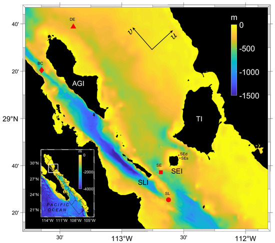
Figure 1.
Study region with bathymetry provided by the product GEBCO2019, and locations of islands and ADCP moorings used for validation in the midriff region. Island Acronyms—AGI: Angel de la Guarda Island. SLI: San Lorenzo Island. SEI: San Esteban Island. TI: Tiburon Island. ADCP Mooring Acronyms—BC: Ballenas Channel. DE: Delfin Sill. SL: San Lorenzo. SE: San Esteban. The insert shows the boundaries of the 24 subdomains generated to run the model. A coordinate system showing the velocity component u perpendicular to the GoC and the velocity component v along the GoC, is included for reference.
The tides in the GoC are generated by co-oscillation with the Pacific Ocean through the mouth of the GoC [29,30]. These are mixed mainly semidiurnal in the southern and northern regions, mixed mainly diurnal near Santa Rosalía (south of the GIR, where we also can observe an amphidromic point for the semidiurnal tides), and mixed mainly semidiurnal in the GIR. In the GIR, the dominant tidal constituents are the , , and semidiurnal components, with the and diurnal constituents playing less of a role [19,31]. Although tides are baroclinic, the barotropic tide is more energetic, and given that here the model is forced only with tides, a 2D hydrodynamic model can be implemented. This model is described in more detail in the next subsection.
The Great Island Region (GIR) consists of 70 islands separated by channels less than 600 m deep. This study focuses on the GIR and specifically on the region encompassing San Lorenzo Island (SLI), San Esteban Island (SEI), Tiburon Island (TI), and Angel de la Guarda Island (AGI), shown in Figure 1. In the GIR maximum flow speeds, more than 2 m s−1, have been found between the channels formed by the different Islands by observational data, specifically in the San Esteban (SE) sill [32,33]. Peak current speeds of up to 1 m s−1 have been found by numerical models in the channel between SLI and SEI, the channel between SEI and TI (Tiburon Channel), and in the Ballenas Channel, between AGI and the Baja California peninsula [20,34].
2.2. Description of the 2D Hydrodynamic Model
To simulate flow conditions in the GoC, we use a shallow-water model with a flexible mesh, and the Delft-FM model developed by Deltares1, in two-dimensional (2D) barotropic form. The model is forced at the mouth of the GoC with along-track tidal constant estimates at a regional scale provided by Xtrack, based on 75 tidal components [35]. Neither wind nor temperature or salinity gradients were considered in the simulation, as these forcings would induce baroclinic circulations, which are beyond the scope of this study. The General Bathymetric Chart of the Oceans (GEBCO2019) was used as the bottom boundary and coastline and has a spatial resolution of 450 m. The study region’s bathymetry is shown in Figure 1.
Delft-FM solves the incompressible Navier–Stokes equations under shallow water and Boussinesq approximations. With these approximations, we can assume that the vertical accelerations are negligible in the momentum equations; we replace the vertical momentum equation with the hydrostatic balance and compute the vertical velocities from the mass conservation equation. As mentioned above, temperature and salinity changes are neglected, and so are density gradients.
We generated a triangular finite-element mesh and refined it near the boundaries. The element edge sizes vary from around 500 m at its coarsest resolution to around 10 m at its finest resolution, with the finest regions adapting to the coastline. Thus, here, the limitations of the model near the coast are related to the bathymetric and coastline assumptions of GEBCO2019 and not the mesh size. Figure 2 shows a close-up of the mesh generated on the Southwestern corner of SEI, in the channel between SEI and SLI. The triangular mesh changes gradually in resolution, from the coarsest in the deep regions to the finest near the coastlines.
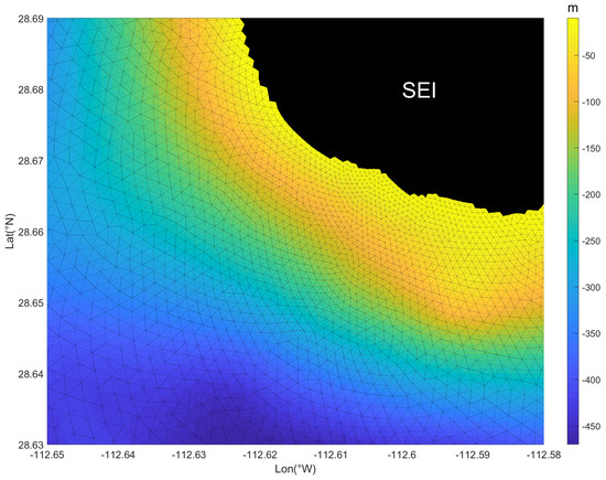
Figure 2.
Central computing subdomain with part of SEI, showing the grid refinement near the shoreline.
The model equations are discretized using the Finite-Volume method on a C-staggered grid [36], where we compute the velocities normal to the cell faces and the scalar variables at the cell centers. The vertical coordinate may be terrain-following coordinate, the Cartesian coordinate z, or a hybrid system, with z being the Cartesian vertical coordinate in physical space and being defined as
where is the free surface elevation above the still-water reference plane , and H is the total water depth; by definition, at the free surface and at the bottom. In the 2D model, without wind forcings nor temperature or salinity gradients, only one layer is implemented. Implicit time integration is performed with the -method following [37], but the advection terms are solved explicitly. The results reported here were obtained with D-Flow FM Version 1.2.110.68930M downloaded from https://svn.oss.deltares.nl/repos/delft3d/tags/delft3dfm/67706/ (accessed on 12 March 2022), and compiled with ifort with support for MPI, PETSc, and METIS, at the high-performance computer of the Mexican National Laboratory of the Southwest (Project No. 202101009n). The numerical model runs in parallel using 24 processors. The inset of Figure 1 shows the 24 computational subdomains.
2.3. Energy Characterization
Velocity data are the primary factor in determining the quality of a site, and they are required in order to evaluate its potential [38]. We ran a simulation for the year 2020 to map and analyze the annual mean speed (), the annual mean of the spring tide maxima (), and the Tidal Power Density ():
where is the instantaneous speed, is the spring tide maximum observed during the simulated year of 2024, and = 1024 kg m−3 is the water density. The yearly averaged TPD is defined as
with . Here, is the total number of hours in the simulation.
Besides the yearly averaged and the mean for spring tidal maxima, , it is possible to compute a threshold , defined here as the mean considering only the values above 50 W m−2. This technical threshold corresponds to a low speed limit or a speed threshold, , of m s−1, typical of most tidal energy devices [20]. When computing the and its yearly mean, , it is important to determine the percentage of time when we are above this threshold as well.
2.4. Tidal Flow Asymmetry and Tidal Phase Asymmetry
The tidal asymmetry was analyzed in detail, as tidal asymmetries have an important effect on . Tidal wave deformation leads to an unequal duration of the rise and fall of the tide (tidal elevation changes), as well as a difference in the duration and magnitude of flooding and ebbing currents (horizontal tidal motion) [39,40]. From a device perspective, it is important to select sites where the tidal currents have equal magnitude in the flood and ebb phases of the tide, i.e., where the tidal cycle is as symmetric as possible. In many locations of the GoC, and due to the general GoC orientation with respect to the Geographical North, a flood tide will present a northwest direction, and the ebb tide will be in the southwest direction. However, the presence of islands can change the dominant tidal directions, as we see in this work.
The Tidal Flow Asymmetry is the ratio between the flood and the ebb mean tidal speeds, given by
where and corresponds to mean tidal speeds for each period. Therefore, a indicates a flood-dominant tide and an ebb-dominant tide.
To evaluate how will be affected by tidal asymmetry, we calculate the relative current speed asymmetry, , as well as the relative asymmetry, , as
Furthermore, Tidal Phase Asymmetry () indicates the direction of tidal asymmetry and is dominated by the phase relationship between the principal semidiurnal tidal current () and its first harmonic () [41]; hence, is given by
We consider only the astronomical tidal constituent and its harmonic in the numerical experiments for conceptual simplicity. Observations show that is the dominant tidal constituent and generally is the dominant shallow water (nonlinear) constituent in the study area; therefore, the effect of other tidal constituents on tidal deformation is minor (See Supplementary Material).
If the Tidal Flow Asymmetry () differs significantly from 1, then the power generation will be large during one half of the tidal cycle and weak during the other half. This has implications for the total power production [42], as well as for grid management. The characteristics during flood and ebb-dominant conditions are discussed in Section 3.3.
2.5. Data Used for Model Validation
To ensure that the model predicts accurately the hydrodynamic conditions in the GoC, and in particular in the GIR, tidal levels and flow speeds were validated against tidal gauge and ADCP measurements.
Four tidal gauge sites were selected along the gulf obtained from the tidal gauge network maintained by the Center for Scientific Research and Higher Education at Ensenada (CICESE); the tidal range graphs can be consulted from redmar.cicese.mx. Tidal gauge measurements are taken by sea level sensors, and therefore, only provide sea elevation time series, whereas the ADCP data provide current velocity time series over the water column at a single horizontal (geographical) location. Figure 3 shows the tidal gauge locations. The sensors used are located along the Baja Californian Peninsula, and not on the region of interest, i.e., the GIR, as tidal elevation measurements have little sensitivity to local coastline/bathymetry approximations. It is worth noting that including more tidal gauge measurements would not really increase the robustness of the model validation.
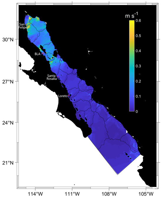
Figure 3.
Annual mean speed (m s−1) predicted by the model. The thin black lines show the model subdomains used for computational purposes, as described in the grid generation and analysis Section 2.2.
The ADCP data used for model validation are different from the data presented in Section 2.7 at the end of this section; they were obtained in a prior project led by CICESE that was undertaken between 2002 and 2006 (see Acknowledgments), during which four ADCPs were deployed in four GoC sills: the San Lorenzo (SL), the San Esteban (SE), the Ballenas Channel (BC), and the Dolphin (DE) sills. BC and DE sills are on the northern side of the GIR, while SL and SE sills are on the southern side. The speed measurement precision is approximately 0.1 m s−1, according to the instrument specifications. The data from these experiments have been used in several other publications; see, for example, [32,43] and references therein. It is worth noting that more ADCP data are available in the San Jorge and Adair Bays [44]; however, current speeds are very sensitive to local coastline/bathymetry approximations, and therefore, it would not be useful to include validation data outside the region of interest, i.e., the GIR. Also, the ADCPs at the sills were deployed for several months and are ideal data for model validation. Figure 1 shows the ADCP locations, both those used for model validation presented here, as well as the two moorings SEd and SEs near San Esteban Island used to complement the model analyses that are discussed at the end of this section.
2.6. Model Validation: Modeled Tidal Signal Predictions against Coastal Tidal Gauge Measurements and against ADCP Tidal Data at GIR Sills
We performed a tidal decomposition analysis of observations and model predictions using t_tide [45]. The model’s accuracy is then quantified using the Root Mean Square Error, , and the Correlation Coefficient, , between X and Y (Table 1), where X corresponds to model predictions and Y to observations.

Table 1.
Tidal gauge locations, [m] and correlation coefficient between model and tidal range data, organized from North to South: San Felipe, Bahia de Los Angeles (BLA), Santa Rosalia, and Loreto.
Figure 4 shows the amplification of tidal range towards the north of the GoC from 1 m in Loreto to 5 m in San Felipe, and we also can observe that the model reproduces the spring–neap tide periods, as well as the diurnal and semidiurnal tides. It is worth noting that the tidal range maximum is around m at the mouth of the Colorado River Delta, on the western side of the head of the Gulf of California [15]. Table 1 shows that there is a good correlation between the time series and an acceptable in the four sites used to validate the water elevation predictions against tidal gauge observations: San Felipe, Bahia de los Angeles (BLA), Santa Rosalia, and Loreto. To assess the model performance in more detail, we compare the amplitudes and phases of the modeled and observed and tidal components in Table 2. There is a good agreement between model (mod) and observations (obs) of the amplitudes and , with an of m and m, respectively. The corresponding between the modeled and observed phases of and was 17° and 4°, respectively. We observed that the modeled phase of the tidal component in the Loreto tidal gauge station showed a significant difference from the observations, and the same is true for the phase of the tidal component.
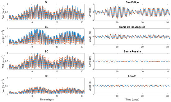
Figure 4.
Time series of observed (blue continuous line) and modeled (red dashed line) flow velocity (left panel) and tidal levels (right panel) for two spring–neap cycles.
Table 2.
Amplitudes [m] and phases [°] of the and tidal components, extracted from the model predictions and the tidal gauge observations.
Furthermore, tidal flow velocity predictions were verified against measurements provided by ADCP instruments at four sill sites in the GIR: San Lorenzo (SL) sill, San Esteban (SE) sill, Ballenas Channel (BC), and Delfin sill (DE) (see Figure 4). The locations of the ADCPs are shown in Figure 1 and the campaigns and the data are thoroughly described in [43].
A tidal analysis was performed on the observed data to extract the astronomical tides. The tidal analysis was performed with t_tide, and the tides were reconstructed with t_predict for the year 2020 [45]. This prediction was then compared with the tidal flow time series reproduced with the model. Table 3 shows a detailed comparison between the observed (obs) and modeled (mod) speeds including the mean speeds (), the maximum speed (), and the spring tidal mean speeds ().
Table 3.
Observed and modeled speeds [m s−1] with means computed over 365 days of simulation. The Root Mean Square Error, [m s−1], the relative error, [%], and the Pearson correlation coefficient, [], quantify the agreement between model and observations.
The between and varies between and m s−1 and the between 16% and 20%, with the largest occurring at the BC sill. Maximum observed current speeds of m s−1 and m s−1 were found in the SL and SE sill, respectively. For the modeled data, SL and BC sill were also the most energetic. DE sill shows the lowest current speed values in both numerical and modeled data, with a of m s−1 and of m s−1.
We tested how the tidal model prediction changed with the use of different tidal constituents, comparing the model predictions with 35 and 59 tidal constituents and observations at the sills. We observed that the and the decreased when using the largest number of constituents (See Appendix Table A1 and Table A2). For example, for SL mooring an of 16% was obtained using 59 tidal constituents for the tidal signal reconstruction, compared with a value of 25% using 35 tidal constituents. From here onwards, we select the signal reconstruction based on the full year of simulations from 2020 and use 59 tidal constituents for the reconstructed tidal signal.
We calculated the corresponding to an instantaneous speed equal to m s−1 for SL, SE and BC sills. However, a lower threshold of m s−1 was chosen in DE because a lower tidal current speed was found in the sill. We also calculated the for the observed and modeled data at the four sills and performed a statistical analysis to evaluate the model accuracy on the energy characterization (Table 4). We observed a greater of in the SE sill for , and a of for on BC. In general, we observed an overestimation of the model data in SL, BC and DE sills and an underestimation in the SE sill. Overall, we found a good agreement between the model predictions and the observations at the sills.
Table 4.
Average speed [m s−1] and tidal power density [W m−2] thresholds (th) for the observations (obs) and the model (mod), together with their respective relative errors, [%], and Pearson coefficient [], at the four sill moorings.
2.7. Tidal Asymmetry Analysis from In Situ Measurements
Although the tidal analysis and the tidal energy characterization with the Delft-FM model validated at the four coastal tidal gauges and the four ADCP data at GIR sills are the main focus of this paper, we recognize that some coastal regions cannot be assessed in detail with the model due to coastline or bathymetric limitations very close to the shore. At locations that are not within the model domain, but for which we have ADPC measurements, in situ data cannot be used for model validations, but the observations can complement the analyses and results obtained from the numerical model. Therefore, we used the current data of two ADCP moorings in SEI at different depths (see Figure 1 for location) to complement the Energy characterization.
At SEd, the mooring was placed at 60 m for a period of 75 days (4 August 2021 to 19 October 2021), while at SEs the mooring was placed at 25 m for a period of 150 days (3 October 2019 to 1 April 2020). Current observations were taken with sampling intervals of hours, with an average sampling period of 60 s and a vertical resolution of 100 cm. A tidal decomposition analysis was performed using the t_tide package [45]. Vertical profiles were analyzed to describe the energy resource along the water column and vertical distribution of tidal asymmetry. Flood and ebb periods where identified at each mooring by calculating the velocity component, v, along the axis from the geographical North, which corresponds approximately to the longitudinal axis of the GoC (see Figure 1). A value of will then indicate the flood period (towards the head of the GoC), while a value will indicate the ebb period (towards the mouth of the GoC). A time average of the speed was calculated during the flood and ebb period to calculate and , and calculations of the and indices were performed.
3. Results and Discussion
3.1. Annual Mean Speed and Tidal Power Density
Figure 3 shows the annual mean flow speed of the GoC predicted by the 2D model. We observed minimum speed currents of m s−1 at the entrance of the GoC, where we have the maximum depths and the widest transversal cross-section of the Gulf. As we move north of the GoC’s shallower depths and narrower cross-sections, the mean flow speeds predicted by the model increase to 0.5–0.6 m s−1 in the GIR and the Upper Gulf of California. It is clear that the presence of the islands, straits, and the constrictions formed by them, plays an important role in the mean flow speeds in the GIR. At the Upper Gulf of California, we also observe maximum mean speed values due to the amplification of the tidal range that was mentioned in Section 1. These two regions also have been identified as potential sites for tidal energy exploitation by previous authors [14,20,34]. Magar et al. [20] found maximum speed values close to 1.1 m s−1 for the annual mean of the spring tide maxima () in the channels formed by the different islands, specifically around SEI and SLI. Here, we found values up to 0.6 m s−1 of the around the same locations; however, due to the higher bathymetry resolution used in the present work, we observed a better representation of these maximum values around the islands and shallow regions. The distribution and magnitude of maximum current speed values can vary significantly with the choice of the bathymetry product, and the number of tidal constituents used [18]. We observed that the use of a larger number of tidal constituents improved model prediction and resource characterization in the region.
The annual mean tidal power density, being proportional to the cube of the speed, follows the same pattern distribution that we observe in Figure 3 for the annual mean current. These results agree with those obtained by [20] with the HYCOM model, which also show the GIR and the Upper Gulf of California near the mouth of the Colorado River as the two most relevant regions for tidal current energy resource exploitation. In the rest of this work, we focus on the GIR. We analyze in more detail the speeds and tidal power densities in that region, as well as the tidal asymmetry using several indexes, and we assess the effects of tidal asymmetry on tidal energy resource exploitation. We also present some results based on in situ measurements, which complement the results obtained with the numerical model.
3.2. Annual Mean of Threshold Speeds, , and Annual Mean of Threshold ,
A measure of the technical resource can be obtained by considering speeds above an energy-producing lower threshold. A of 64 W m−2 was selected here, corresponding to instantaneous speeds equal to m s−1.
Locally, we observed that tidal flow is strongest at headlands, in the Tiburón channel between SEI and TI, in the Infiernillo Channel between TI and the mainland, as well as in the Ballenas Channel between AGI and the Peninsula. Other hotspots with large are observed at various locations between the islands (see Figure 5). The high tidal energy resources within channels is caused by Venturi acceleration effects at both vertical and horizontal constrictions. A vertical constriction occurs when the water depth changes abruptly at sills or canyons.
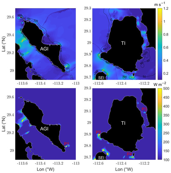
Figure 5.
Maps for the two largest islands in the GIR, AGI, and TI. (Upper panels): annual mean of threshold speed, [m s−1]. (Lower panels): annual mean threshold Tidal Power Density, [W m−2].
The upper panels of Figure 5 show around AGI and TI, as well as the 50 m and 100 m bathymetry contours delimiting the depth ranges for the installation of bottom-mounted tidal energy devices. Maximum values of current speeds were observed near the 100 m and 200 m bathymetry contour, and we observed current speeds up to 1 m s−1 at the northern end of Ballenas Channel, where abrupt changes in bathymetry are present, and at the headland on the east side of the AGI. TI also shows strong currents at the headlands around the island, specifically on the eastern side of the island, in the Infiernillo Channel, where we observed currents up to m s−1. On the western side of TI, we observed tidal current speeds of up to m s−1 around the headlands, these current speeds are caused by bathymetric constrictions resulting from the presence of smaller islands (e.g., SEI). The lower panels of Figure 5 show the corresponding to the . Because the is proportional to (see Equation (4)), we can expect maximum values at the same locations as the contour maps of . We then select hot spots for energy exploitation based on the speed threshold and a minimum water depth, and analyze how important the tidal asymmetry is at those hot spots. Many potential points meeting the current speed threshold were found around AGI and TI, but they were located at 100 m depth or more. This would not be a problem for floating tidal energy devices, but for bottom-mounted devices, such as those discussed in [20], for example, depths above 100 m are outside the devices’ water depth specifications. Here, we assumed devices will be bottom-mounted and in shallow waters to reduce costs, and therefore, depth is the main limitation for tidal energy exploitation in this region. Also, tidal asymmetry is possibly less of an issue for floating tidal energy devices, because tidal asymmetry drives sediment transport and sediments can damage the turbines, but on the sea surface, the impacts of sediments on the device are less of a concern.
There are two smaller islands that present strong currents in the GIR, these islands are SEI and SLI. The upper panels of Figure 6 show the around SEI and SLI, and 50 m and 100 m bathymetry contours. We found maximum annual mean threshold speeds of up to 1 m s−1 at the east and west sides of SEI, located specifically at the headlands around the island. For SLI, we found a maximum current speed of 0.6 m s−1 at the headlands located in the south, as well as the channels between the smaller islands located north of the island. To assess tidal asymmetry and its relation with TPD around AGI and TI, we selected site P1 near AGI and sites P2, P3, and P4 near TI, shown in Figure 5. We can impose the same requirements of and depth as on the larger islands (AGI and TI) and select hot spots P5 to P8 for SEI and P9 to P12 for SLI, shown in the lower panels of Figure 6. For SEI and SLI, the water depth was not a limitation to select hot spots because all the locations with high are within the 50–100 m depth contours.
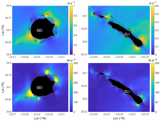
Figure 6.
Maps for SEI and SLI. (Upper panels): annual mean threshold speed, [m s−1]. (Lower panels): annual mean threshold Tidal Power Density, [W m−2].
Energy characterization at the selected hot spots is summarized in Table 5. We selected P1, P2, and P4 at around 30 m depth, with a of 300 to 400 W m−2, corresponding to a of 0.8 m s−1. We also observed a different hot spot at the Infiernillo Channel in TI. Here, we selected P3, with a depth of 3 m; however, we can expect uncertainty for the depth in this region due to bathymetry limitations in shallow regions. The points selected in SEI were the most energetic, P5 to P8, with a value of around 1 m s−1. These hot spots were around 30 to 40 m depth and presented the greater number of days above the imposed threshold, from around 240 days on average, representing a of the year with an extractable resource. It is worth mentioning that, overall, P8 presented the largest of 1026 W m−2, with of the year above the threshold. Finally, hot spots P9 to P12 around SLI were the least energetic, with a value of around 0.7 m s−1 and the smallest number of days above the threshold. Numerical models provide high temporal and spatial resolution to select potential sites and perform further characterization of details.
Table 5.
Tidal asymmetry characterization at the hot spots around the islands in the GIR.
3.3. Tidal Asymmetry Analysis
Tidal Phase Asymmetry, , was defined (see Equation (9) in Section 2.4) in terms of the principal semidiurnal tidal current M2 and its first harmonic M4. In regions where these tidal components are strong compared with other tidal harmonics, a value from 0° to 90° and 270° to 360° will result in a flood-dominant tide; on the other hand, a value from 90° to 270° indicates an ebb-dominant tide. Therefore, when the tide is neither flood- nor ebb-dominant, i.e., when the tidal flow is symmetric, we expect a of around 90° or 270°. Table 5 shows the value of for each hot spot selected in the GIR.
The Tidal Flow Asymmetry, , defined in Equation (6) of Section 2.4, is a measure of the relative importance of the flood vs. the ebb mean current speeds. Figure 7 shows a map around AGI (left panel) and TI (right panel), with contours and a schematic of the general residual circulation generated by the tidal asymmetry. Figure 8 shows similar maps for SEI (on the left) and SLI (on the right). A value close to indicates a strong flood-dominant tidal flow, while a value close to 0.2 corresponds to an ebb-dominant tidal flow, and a value close to 1 corresponds to a symmetric tidal flow. It is clear that tidal asymmetry is more important in shallow regions, around headlands, and in the channels between the islands. Contours of large appear to be located in symmetrical regions, delimited by the flood and ebb-dominant regions.
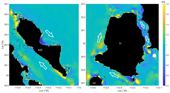
Figure 7.
maps around AGI (left panel) and TI (right panel), with contour lines of the . The white arrows represent a schematic of the direction of the residual circulation around each of the islands.
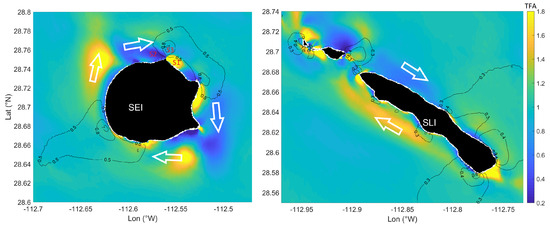
Figure 8.
Maps of around SEI (left panel) and SLI (right panel) with contour lines of the . Schematics of general residual circulation around SEI and SLI are also shown.
We selected three strategic points (see Figure 8) to evaluate the resource with a flood-dominant flow (S1 case), ebb-dominant flow (S2 case), and a symmetrical tide (S3 case). Figure 9 shows time series of U and (see Equation (4)) for a one-month period at S1, S2, and S3, highlighting the values of speed and for flood and ebb periods. The asymmetry of the current speed during the flood and ebb tides in S1 and S2 is clear, whereas, for S3, the current speed during flood and ebb tides is almost symmetrical. Given that the is directly related to the cube of the speed, the asymmetry in velocity is translated into a much stronger asymmetry in tidal power density. For example, at S1 and S2, we found an of 16.2% and 16.6%, respectively, which represents a relative asymmetry in tidal power density, , of 77% and 87%, respectively. On the other hand, for S3, we found an of 6.2%, which translated into an of 17%. We can also point out that at S3, the current speed is strong, close to to 2 m s−1 in spring tides, compared with a maximum of 1 m s−1 in spring tides at S1 and S2.
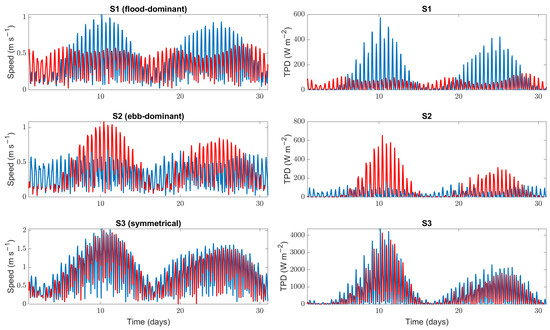
Figure 9.
Current speed (left panels) and TPD (right panels) for S1 (flood dominant tide), S2 (ebb dominant tide), and S3 (symmetrical tide). The blue line indicates flood periods and red lines ebb periods.
Table 5 shows details of and at the selected P1 to P12 within hot spot areas identified in the GIR. For P1 in the southeastern edge of AGI, we observed a slightly ebb-dominant tide with a value of 118 and a value of 0.94, which indicates a symmetrical tide, causing only a 6% . Around TI, the values of P2, P3, and P4 indicate a flood-dominant tide; however, the values indicate an ebb-dominant tide at P3 and P4 and a symmetrical tide at P2 (5% in ). Although the at P2 and P4 are 85° and 80°, hence closer to 90°, this indicates that there may be factors affecting tidal asymmetry in coastal regions other than the and phase relationship. For example, other tidal components may also play a role in the Tidal Phase Asymmetry, possibly because the hot spots being analyzed are not aligned with one another but located at different island coastal locations, and the tidal wave gets distorted by the presence of the islands, affecting phase lags between hot spots. P5, P6, and P8 (selected around SEI) show a symmetrical tide with TFA values of 1.06, 0.97, and 0.94, respectively, as well as an value of less than 10% and a of less than 30%. P9 was selected between a group of small islands south of SLI and presented the largest tidal asymmetry for both and with an ebb-dominant tide, causing an of 27%, and an of 62%. At P10, P11, and P12, we observed a symmetric tide, with TFA values close to 1 and an of less than 10%.
3.4. Residual Circulation in the GIR
We calculated the mean of the current speed velocity over the simulation period of one year, and we observed anticyclonic circulations of the residual currents around AGI, TI (Figure 7), and around SEI and SLI as well (Figure 8). This anticyclonic circulation is deduced from the vectorial representation of the mean velocity currents for the full year of simulation—the figures of this vectorial representation for the four GIR islands considered in this study are included in the Supplementary Materials. The direction of the annual residual current circulation generally coincides with the dominant flood–ebb direction of the tidal currents around the islands, as we discuss in the following. For AGI, a flood-dominant tide is observed at the west side and at Ballenas Channel, consistent with a northward circulation, while an ebb-dominant tide is observed at the east side of the island, consistent with a southward circulation (white arrow in Figure 8). In TI, a northward circulation is observed at the north and southwest sides of the island, coinciding with a flood-dominant tide and a strong southward circulation on the east side of the island in the Infiernillo Channel, consistent with a strong ebb-dominant tide. This pattern is also observed in SEI and SLI (Figure 9). The circulation in the GIR has been previously studied by [46]; they calculated the superposition of the Euler and Stokes residual current, namely the Lagrange residual current, and they also observed an anticlockwise circulation around AGI and TI. Here, we extended the analysis to SEI and SLI and show this anticlockwise circulation is also observed around these two islands.
3.5. Analysis of In Situ Measurements near SEI
Two locations, SEd and SEs, were selected near SEI to evaluate the tidal energy resource using moored ADCPs (see Figure 1 for location). For SEd, the ADCP was placed at 60 m for a period of 75 days, whereas, at SEs, the ADCP was placed at 25 m for a period of 150 days, as discussed in Section 2.7. Figure 10 shows the speed profiles along the vertical for a period of 15 days for SEd (top subplot) and SEs (bottom subplot), as well as the depth-averaged northward component of the velocity aligned with the axis of the GoC, v [m s−1], showing flood () and ebb periods (). The harmonic analysis was carried out with t_tide, and some cells were removed from the surface and the bottom to avoid contamination from noise.
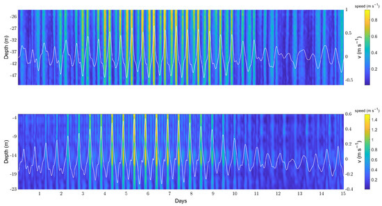
Figure 10.
Speed profiles of a neap–spring tidal cycle for SEd (upper panel) and SEs (low panel). The white line shows v, the depth-averaged velocity component along the GoC.
We can observe the spring tide period between days three and ten of the monitoring campaign, when the SEd current speed reaches 1 m s−1 during flood periods and the maximum values were found near the surface. The current speed maxima are less energetic during ebb periods. We also note that the flow speeds decrease with water depth from the surface to the bottom. At SEs, we observe current speeds of up to 1.6 m s−1 in spring tide. Maximum values were found close to the surface and at around 14 to 15 m from the surface, with a decrease in velocity close to the bottom. The velocity profiles at SEs also show a strong tidal asymmetry, with larger current speeds during flood periods. Figure 11 shows the for the same periods. values between 250 and 400 W m−2 are observed in SEd, and up to 1200 W m−2 in SEs. Although for SEs the energy resource appears to be greater than SEd, there is a strong asymmetry in the resource. From the above, we also conclude that the depth of the maximum speed along the vertical will depend on the mooring location. This can have important implications for tidal device siting and the type of tidal device that is most appropriate for a given location. This analysis shows the importance of the vertical distribution of the current speed in the characterization of the tidal energy resource.
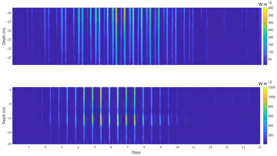
Figure 11.
TPD profiles for a 15-day period at SEd (upper panel) and SEs (low panel).
Time-averaged speed vertical profiles, , and time-averaged speed for flood and ebb periods are shown in Figure 12 for SEd (left panel) and SEs (right panel). For SEd mooring, we found values of increased with depth, from 1.2 on the surface (18 m) to 1.3 at the bottom (50 m). On the other hand, for SEs, a more complex pattern of was observed: we found a value of of 1.5 near the surface (4 m), increasing with water depth to 2.1 at around 13 m and decreasing again to 1.5 on the bottom at 23 m. This highlights the importance of evaluating tidal asymmetry along the water column, as well as the differences in shallow and depth locations. Tidal Phase Asymmetry was also calculated, with corresponding value of 88° and 7° for SEd and SEs, respectively, indicating a flood-dominant tide as well. Overall, and values show a flood-dominant tide in both mooring locations, with a stronger tidal asymmetry in SEs.
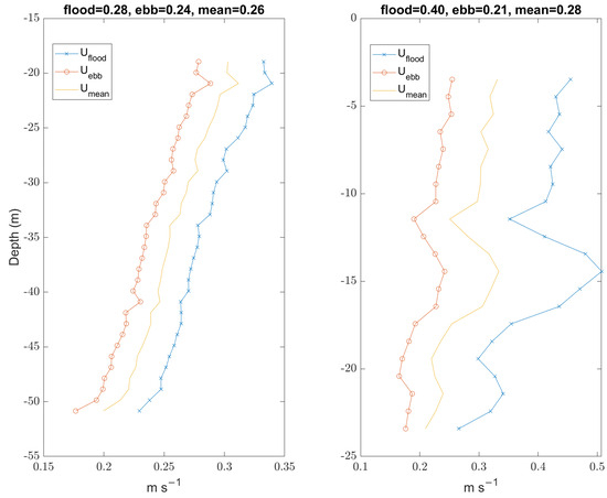
Figure 12.
Vertical profile for SEd (left panel) and SEs (right panel). Vertical averages of speed for flood and ebb periods are shown on the top of the panels.
To evaluate how tidal asymmetry will affect the available power, and were calculated using Equations (7) and (8), respectively. For SEd, close to the surface, we found values of of 16%; then, increases with depth, but not by much, to values of 20 to 25% near 50 m water depth. A 30% velocity asymmetry can translate into a 100% tidal power density asymmetry, as reported in [24], and this highlights the importance for developers to find (and avoid) the regions of highest asymmetry for the tidal current. It is clear that tidal asymmetry is greater at SEs than at SEd, at least at the depths where we measurements for both locations. The tide is flood-dominant in SEs, with a minimum of around 42% near the bottom and a maximum of 80% at around 14 m depth from the surface. The minimum value of is still substantial, given that it corresponds to an of 145%.
4. Conclusions
A hydrodynamic 2D model of the GoC was developed to evaluate the tidal energy resource in the GIR. The GIR is the midriff region, where several large and small islands are found, and in combination with a complex bathymetry, large flow velocities are observed, specifically around islands, in channels between the islands, and near island headlands. The sites with the highest speeds agree in general with those identified in previous studies, but the increased resolution of the mesh used here leads to a more thorough characterization analysis. A technical threshold for the speed and a minimum depth was imposed to select hot spots around the islands and evaluate tidal resources and tidal asymmetry, which has important implications for tidal energy resource exploitation. Depth was found to be an important limiting factor in some regions, such as AGI, where we observed current speeds of up to 1 m s−1; however, these hot spots were found at depths of around 200 m. On the other hand, we found several hot spots in the Infiernillo Channel, a very narrow channel located between TI and the mainland; the spots were less than 8 m deep, although this is known to be a shallow region, and limitations in bathymetry could underestimate depth values. Overall, we found that the San Esteban Island is the best site in the GIR for energy extraction, since the most energetic hot spots were found around this island. Hot spots P5 to P8, for example, have speeds above threshold for 70% of the year. Here, the threshold speeds can be as large as 1.1 m s−1, representing a tidal power density of 1026 W m−2. Of all the GIR sites analyzed here, those within Tiburón Channel would be the most suitable for siting of tidal energy converter devices.
Two indexes were used to evaluate tidal asymmetry. is a measure of tidal asymmetry in terms of the M2 and M4 tidal component phases, whereas is the flood−ebb flow ratio. maps of the GIR showed that tidal asymmetry is stronger in shallow regions, around headlands, and in channels between the islands. We also observed, from the contour lines, that symmetrical regions exhibit maximum flow speed values. Regions with strong ebb- or flood−dominant tide present a difference between flood and ebb flow speeds in relation to the mean speed of 16% and can translate into a 70 to 80% asymmetry in tidal power density, . This would affect the efficiency of energy conversion of tidal energy converters.
The 2D model provides information with high spatial and temporal resolution to evaluate the resource and select potential sites for energy extraction. However, the bathymetry and the coastline representations have a coarse resolution in comparison with the model mesh, which therefore means the results are, to some extent, theoretical. We observed with this model that one possible extension of the work is to analyze the sensitivity of the results to different coastline and bathymetry assumptions, especially for small island regions where this can have a significant effect. Also, wind-induced residual currents can have important seasonal effects, which cannot be analyzed with tidal forcings alone. These two limitations deserve to be investigated more thoroughly with the 2D model.
Due to the bathymetry and coastline choices, in shallow regions, it is necessary to further evaluate the sites with in situ measurements. Thus, we complemented the model results obtained with ADPC measurements at two coastal locations, one shallow (SEs) and one deep (SEd), near SEI. We found stronger current speeds for SEs of up to 1.6 m s−1, representing a tidal power density of 1200 W m−2. However, in accordance with model results, this shallower point exhibits a larger tidal asymmetry, with a depth-averaged current speed in flood and ebb periods of 0.4 m s−1 and 0.21 m s−1, respectively, resulting in a strong flood-dominant tide. Tide asymmetry also changed along the water column, with a maximum value of close to 80% at 15 m depth at SEs, where a stronger current velocity was also observed. In contrast, at SEd, a 16–20% was observed along the water column. The in situ data show the importance of vertical characterization, as maximum values can be found at different heights above the seabed depending on location, which is important for device selection. This vertical characterization will be investigated in future model implementations, as it is beyond the capabilities of the 2D model.
Finally, we recommend that tidal energy converters be placed in regions where the tide is as symmetric as possible, so this should be taken into account together with the and other criteria, such as environmental and social impacts.
Supplementary Materials
The following supporting information can be downloaded at: https://www.mdpi.com/article/10.3390/jmse12101740/s1, Figure S1: Residual circulation around SEI (left) and SLI (right). Figure S2: Residual circulation around AGI (left) and TI (right). Figure S3: SEp’s Tidal ellipse velocity components along the semi-major (left) and semi-minor (middle) axes, and tidal ellipse inclination (in degrees) with respect to East. Figure S4: SEs’ Tidal ellipse velocity components along the semi-major (left) and semi-minor (middle) axes, and tidal ellipse inclination (in degrees) with respect to East.
Author Contributions
Conceptualization, A.B.-R. and V.M.; methodology, A.B.-R., V.M., M.L.-M. and J.D.D.B.; software, A.B.-R. and V.M.;validation, A.B.-R.; formal analysis, A.B.-R., V.M., and M.L.-M.; investigation, all co-authors;data curation, A.B.-R. and M.L.-M.; writing—original draft preparation, A.B.-R. and V.M.; writing—review and editing, A.B.-R., V.M., M.L.-M. and J.D.D.B.; visualization, A.B.-R. and M.L.-M.; supervision, V.M.; project administration, V.M.; funding acquisition, A.B.-R. All authors have read and agreed to the published version of the manuscript.
Funding
This research was funded by a CONAHCYT PhD scholarship grant No. 29347, awarded to the first author. The APC was partly funded by CICESE and partly by GEMlab. We also acknowledge MDPI’s Institutional Open Access Program with the University of Edinburgh. The fieldwork campaigns were supported by CICESE’s internal project No. 621177, by SENER-CONACYT grant No. 249795, within the project “CeMIE-Océano” (2017–2021) and project G33464-T (2000-2005) funded by CONAHCYT. We thank the three anonymous reviewers for their comments, which significantly improved the manuscript. The authors thankfully acknowledge computer resources, technical advice, and support provided by the Laboratorio Nacional de Supercómputo del Sureste de México (LNS), member of the CONAHCYT National Laboratories Group, with project No. 202101009n.
Institutional Review Board Statement
Not applicable.
Informed Consent Statement
Not applicable.
Data Availability Statement
The model output data used for this publication is provided in postprocessed form in a zenodo repository, together with the postprocessed in situ measurements around San Esteban Island.
Acknowledgments
We thank Markus S. Gross (deceased on 25 January 2022) for setting up the Delft-FM model used for this research in the LNS supercomputer and for carrying out the initial model validations.
Conflicts of Interest
The authors declare no conflict of interest. The funders had no role in the design of the study; in the collection, analyses, or interpretation of data; in the writing of the manuscript, or in the decision to publish the results.
Abbreviations
The following abbreviations are used in this manuscript:
| MDPI | Multidisciplinary Digital Publishing Institute |
| Delft3D FM | Delft3D Flexible Mesh |
| GoC | Gulf of California |
| ADCP | Acoustic Doppler Current profiler |
| TPD | Tidal Power Density |
| GIR | Great Island Region |
| SEs | San Esteban Shallow |
| SEd | San Esteban deep |
| TECs | Tidal current energy converters |
| SLI | San Lorenzo Island |
| SEI | San Esteban Island |
| TI | Tiburon Island |
| AGI | Angel de la Guarda Island |
| GEBCO | General Bathymetric Chart of the Oceans |
| Annual mean speed | |
| Annual mean of the spring tide maxima | |
| Maximum speed | |
| Yearly average TPD | |
| Mean TPD for spring tidal maxima | |
| Speed threshold | |
| Observed speed | |
| Modelled speed | |
| Relative asymmetry of the current speed | |
| Relative asymmetry of the TPD | |
| Yearly mean TPD threshold | |
| Tidal Flow Asymmetry | |
| Tidal Phase Asymmetry | |
| Mean tidal speed in flood period | |
| Mean tidal speed in ebb period | |
| CICESE | Center for Scientific Research and Higher Education at Ensenada |
| Root Mean Square Error | |
| Relative error | |
| Pearson correlation coefficient | |
| BLA | Bahia de Los Angeles |
| SL | San Lorenzo sill |
| SE | San Esteban sill |
| BC | Ballenas Channel |
| DE | Delfin sill |
Appendix A
Appendix A.1
Table A1.
Observed and modeled speeds [m s−1] with means computed over 365 days of simulation. Observed speeds were predicted using 35 tidal components. The Root Mean Square Error, [m s−1], the relative error, [%], and the Pearson correlation coefficient, [], quantify the agreement between the model and observations.
| Mooring | [%] | ||||
|---|---|---|---|---|---|
| SL | 0.40 | 0.39 | 0.11 | 25 | 0.90 |
| SE | 0.46 | 0.34 | 0.16 | 27 | 0.92 |
| BC | 0.35 | 0.41 | 0.10 | 27 | 0.94 |
| DE | 0.17 | 0.19 | 0.05 | 21 | 0.94 |
Table A2.
Observed and modeled speeds [m s−1] with means computed over 365 days of simulation. Observed speeds were predicted using 59 tidal components. The Root Mean Square Error, [m s−1], the relative error, [%], and the Pearson correlation coefficient, [], quantify the agreement between the model and observations.
| Mooring | |||||
|---|---|---|---|---|---|
| SL | 0.38 | 0.39 | 0.07 | 16 | 0.96 |
| SE | 0.41 | 0.34 | 0.11 | 19 | 0.96 |
| BC | 0.36 | 0.41 | 0.08 | 20 | 0.97 |
| DE | 0.18 | 0.19 | 0.04 | 16 | 0.96 |
Note
| 1 | https://oss.deltares.nl/web/delft3dfm/, accessed on 21 September 2024 |
References
- Nicholls-Lee, R.; Turnock, S. Tidal energy extraction: Renewable, sustainable and predictable. Sci. Prog. 2008, 91, 81–111. [Google Scholar] [CrossRef] [PubMed]
- Baker, C.; Leach, P. Tidal Lagoon Power Generation Scheme in Swansea Bay: A Report on Behalf of the Department of Trade and Industry and the Welsh Development Agency; DTI: London, UK, 2006. [Google Scholar]
- Bahaj, A.S. Generating electricity from the oceans. Renew. Sustain. Energy Rev. 2011, 15, 3399–3416. [Google Scholar] [CrossRef]
- Parker, B.B. Tidal Hydrodynamics; John Wiley & Sons: Hoboken, NJ, USA, 1991. [Google Scholar]
- Charlier, R.H. A “sleeper” awakes: Tidal current power. Renew. Sustain. Energy Rev. 2003, 7, 515–529. [Google Scholar] [CrossRef]
- Bahaj, A.; Molland, A.; Chaplin, J.; Batten, W. Power and thrust measurements of marine current turbines under various hydrodynamic flow conditions in a cavitation tunnel and a towing tank. Renew. Energy 2007, 32, 407–426. [Google Scholar] [CrossRef]
- Magar, V.; Gross, M.; González-García, L. Offshore wind energy resource assessment under techno-economic and social-ecological constraints. Ocean Coast. Manag. 2018, 152, 77–87. [Google Scholar] [CrossRef]
- Lewis, M.; Neill, S.; Robins, P.; Hashemi, M.R.; Ward, S. Characteristics of the velocity profile at tidal-stream energy sites. Renew. Energy 2017, 114, 258–272. [Google Scholar] [CrossRef]
- Thiébot, J.; Coles, D.; Bennis, A.C.; Guillou, N.; Neill, S.; Guillou, S.; Piggott, M. Numerical modelling of hydrodynamics and tidal energy extraction in the Alderney Race: A review. Philos. Trans. R. Soc. A 2020, 378, 20190498. [Google Scholar] [CrossRef]
- Ramos, V.; Carballo, R.; Álvarez, M.; Sánchez, M.; Iglesias, G. Assessment of the impacts of tidal stream energy through high-resolution numerical modeling. Energy 2013, 61, 541–554. [Google Scholar] [CrossRef]
- Xia, J.; Falconer, R.A.; Lin, B. Numerical model assessment of tidal stream energy resources in the Severn Estuary, UK. Proc. Inst. Mech. Eng. Part A J. Power Energy 2010, 224, 969–983. [Google Scholar] [CrossRef]
- Iyer, A.; Couch, S.; Harrison, G.; Wallace, A. Variability and phasing of tidal current energy around the United Kingdom. Renew. Energy 2013, 51, 343–357. [Google Scholar] [CrossRef]
- Carbajal, N.; Backhaus, J.O. Simulation of tides, residual flow and energy budget in the Gulf of California. Oceanol. Acta 1998, 21, 429–446. [Google Scholar] [CrossRef][Green Version]
- Hiriart Le Bert, G. Potencial energético del alto Golfo de California. Boletín de la Sociedad Geológica Mexicana 2009, 61, 143–146. [Google Scholar] [CrossRef]
- Marinone, S.; Lavín, M. Residual flow and mixing in the large islands region of the central Gulf of California. In Nonlinear Processes in Geophysical Fluid Dynamics: A Tribute to the Scientific Work of Pedro Ripa; Springer: Berlin/Heidelberg, Germany, 2003; pp. 213–236. [Google Scholar]
- Olivas, J.T.; Campbell, H.R.; Ramos, M.G.S. Feasibility Analysis for a Tidal Energy Pilot Site in the Gulf of California. Asme Int. Mech. Eng. Congr. Expo. 2013, 56291, V06BT07A087. [Google Scholar]
- Hiriart-Le Bert, G.; Silva-Casarin, R. Tidal Power Plan Energy Estimation; Engineering Institute, Autonomous National University of Mexico: Mexico City, Mexico, 2009; Volume 11, pp. 233–245. [Google Scholar]
- Mejia-Olivares, C.J.; Haigh, I.D.; Angeloudis, A.; Lewis, M.J.; Neill, S.P. Tidal range energy resource assessment of the Gulf of California, Mexico. Renew. Energy 2020, 155, 469–483. [Google Scholar] [CrossRef]
- Lavín, M.; Marinone, S. An overview of the Physical Oceanography of the Gulf of California. In Nonlinear Processes in Geophysical Fluid Dynamics: A Tribute to the Scientific Work of Pedro Ripa; Springer: Berlin/Heidelberg, Germany, 2003; pp. 173–204. [Google Scholar]
- Magar, V.; Godínez, V.M.; Gross, M.S.; López-Mariscal, M.; Bermúdez-Romero, A.; Candela, J.; Zamudio, L. In-Stream Energy by Tidal and Wind-Driven Currents: An Analysis for the Gulf of California. Energies 2020, 13, 1095. [Google Scholar] [CrossRef]
- Guo, L.; Wang, Z.B.; Townend, I.; He, Q. Quantification of Tidal Asymmetry and Its Nonstationary Variations. J. Geophys. Res. Ocean. 2019, 124, 773–787. [Google Scholar] [CrossRef]
- Nidzieko, N.J. Tidal asymmetry in estuaries with mixed semidiurnal/diurnal tides. J. Geophys. Res. Ocean. 2010, 115. [Google Scholar] [CrossRef]
- Speer, P.E.; Aubrey, D.G.; Friedrichs, C.T. Nonlinear hydrodynamics for shallow of tidal inlet/bay systems. In Tidal Hydrodynamics; Parker, B.B., Ed.; John Wiley and Sons, Inc.: New York, NY, USA; Chichester, UK; Brisbane, Australia; Toronto, ON, Canada; Singapore, 1991; pp. 321–339. [Google Scholar]
- Neill, S.P.; Hashemi, M.R.; Lewis, M.J. The role of tidal asymmetry in characterizing the tidal energy resource of Orkney. Renew. Energy 2014, 68, 337–350. [Google Scholar] [CrossRef]
- De Dominicis, M.; Wolf, J.; O’Hara Murray, R. Comparative Effects of Climate Change and Tidal Stream Energy Extraction in a Shelf Sea. J. Geophys. Res. Ocean. 2018, 123, 5041–5067. [Google Scholar] [CrossRef]
- Hermawan, S.; Bangguna, D.; Mihardja, E.; Fernaldi, J.; Prajogo, J.E. The Hydrodynamic Model Application for Future Coastal Zone Development in Remote Area. Civ. Eng. J. 2023, 9, 1828–1850. [Google Scholar] [CrossRef]
- Waldman, S.; Bastón, S.; Nemalidinne, R.; Chatzirodou, A.; Venugopal, V.; Side, J. Implementation of tidal turbines in MIKE 3 and Delft3D models of Pentland Firth & Orkney Waters. Ocean. Coast. Manag. 2017, 147, 21–36. [Google Scholar] [CrossRef]
- Gross, M.; Magar, V. Wind-Induced Currents in the Gulf of California from Extreme Events and Their Impact on Tidal Energy Devices. J. Mar. Sci. Eng. 2020, 8, 80. [Google Scholar] [CrossRef]
- Beier, E. A numerical investigation of the annual variability in the Gulf of California. J. Phys. Oceanogr. 1997, 27, 615–632. [Google Scholar] [CrossRef]
- Ripa, P. Toward a Physical Explanation of the Seasonal Dynamics and Thermodynamicsof the Gulf of California. J. Phys. Oceanogr. 1997, 27, 597–614. [Google Scholar] [CrossRef]
- Argote, M.L.; Amador, A.; Lavín, M.; Hunter, J.R. Tidal dissipation and stratification in the Gulf of California. J. Geophys. Res. Ocean. 1995, 100, 16103–16118. [Google Scholar] [CrossRef]
- López, M.; Candela, J.; García, J. Two overflows in the Northern Gulf of California. J. Geophys. Res. Ocean. 2008, 113. Available online: https://agupubs.onlinelibrary.wiley.com/doi/full/10.1029/2007JC004575 (accessed on 19 September 2024). [CrossRef]
- Marinone, S. Tidal currents in the Gulf of California: Intercomparisons among two-and three-dimensional models with observations. Cienc. Mar. 2000, 26, 275–301. [Google Scholar] [CrossRef][Green Version]
- Mejia-Olivares, C.J.; Haigh, I.D.; Wells, N.C.; Coles, D.S.; Lewis, M.J.; Neill, S.P. Tidal-stream energy resource characterization for the Gulf of California, México. Energy 2018, 156, 481–491. [Google Scholar] [CrossRef]
- CTOH. XTRACK, Along track Tidal Constants (2018_01), 2018. Available online: https://www.legos.omp.eu/ctoh/catalogue/?uuid=a9a22957-727e-4450-8243-ff4708021910 (accessed on 19 September 2024).
- Kernkamp, H.W.J.; Van Dam, A.; Stelling, G.S.; de Goede, E.D. Efficient scheme for the shallow water equations on unstructured grids with application to the Continental Shelf. Ocean. Dyn. 2011, 61, 1175–1188. [Google Scholar] [CrossRef]
- Kramer, S.C.; Stelling, G.S. A conservative unstructured scheme for rapidly varied flows. Int. J. Numer. Methods Fluids 2008, 58, 183–212. [Google Scholar] [CrossRef]
- Polagye, B.; Previsic, M.; Bedard, R. Tidal In-Stream Energy Conversion (TISEC): Survey and Characterization of SnoPUD Project Sites in the Puget Sound. In EPRI North American Tidal in Stream Power Feasibility Demonstration Project; EPRI: Washington, DC, USA, 2007. [Google Scholar]
- Pugh, D.T. Tides, Surges and Mean Sea Level; John Wiley and Sons Inc.: New York, NY, USA, 1987. [Google Scholar]
- Friedrichs, C.T.; Aubrey, D.G. Non-linear tidal distortion in shallow well-mixed estuaries: A synthesis. Estuar. Coast. Shelf Sci. 1988, 27, 521–545. [Google Scholar] [CrossRef]
- Pingree, R.; Griffiths, D. Sand transport paths around the British Isles resulting from M2 and M4 tidal interactions. J. Mar. Biol. Assoc. U. K. 1979, 59, 497–513. [Google Scholar] [CrossRef]
- Gooch, S.; Thomson, J.; Polagye, B.; Meggitt, D. Site characterization for tidal power. In Proceedings of the OCEANS 2009, Bremen, Germany, 11–14 May 2009; pp. 1–10. [Google Scholar]
- López, M.; Flores-Mateos, L.; Candela, J. Tidal currents at the sills of the Northern Gulf of California. Cont. Shelf Res. 2021, 227, 104513. [Google Scholar] [CrossRef]
- Bermúdez-Romero, A.; Magar, V.; Gross, M.S.; Godínez, V.M.; López-Mariscal, M.; Candela, J. In-Stream Tidal Energy Resources in Macrotidal Non-Cohesive Sediment Environments: Effect of Morphodynamic Changes at Two Bays in the Upper Gulf of California. J. Mar. Sci. Eng. 2021, 9, 411. [Google Scholar] [CrossRef]
- Pawlowicz, R.; Beardsley, B.; Lentz, S. Classical tidal harmonic analysis including error estimates in MATLAB using T_TIDE. Comput. Geosci. 2002, 28, 929–937. [Google Scholar] [CrossRef]
- Rodríguez, P.A.; Carbajal, N.; Rodríguez, J.H.G. Lagrangian trajectories, residual currents and rectification process in the Northern Gulf of California. Estuar. Coast. Shelf Sci. 2017, 194, 263–275. [Google Scholar] [CrossRef]


Disclaimer/Publisher’s Note: The statements, opinions and data contained in all publications are solely those of the individual author(s) and contributor(s) and not of MDPI and/or the editor(s). MDPI and/or the editor(s) disclaim responsibility for any injury to people or property resulting from any ideas, methods, instructions or products referred to in the content. |
© 2024 by the authors. Licensee MDPI, Basel, Switzerland. This article is an open access article distributed under the terms and conditions of the Creative Commons Attribution (CC BY) license (https://creativecommons.org/licenses/by/4.0/).