Abstract
The mesoscale interaction between sea surface temperature (SST) and wind is a crucial factor influencing oceanic and atmospheric conditions. To investigate the mesoscale coupling characteristics of the Yellow Sea and East China Sea, we applied a locally weighted regression filtering method to extract mesoscale signals from Quik-SCAT wind field data and AMSR-E SST data and found that the mesoscale coupling intensity is stronger in the Yellow Sea during the spring and winter seasons. We calculated the mesoscale coupling coefficient to be approximately 0.009 N·m−2/°C. Subsequently, the Tikhonov regularization method was used to establish a mesoscale empirical coupling model, and the feedback effect of mesoscale coupling on the ocean was studied. The results show that the mesoscale SST–wind field coupling can lead to the enhancement of upwelling in the offshore area of the East China Sea, a decrease in the upper ocean temperature, and an increase in the eddy kinetic energy in the Yellow Sea. Diagnostic analyses suggested that mesoscale coupling-induced variations in horizontal advection and surface heat flux contribute most to the variation in SST. Moreover, the increase in the wind energy input to the eddy is the main factor explaining the increase in the eddy kinetic energy.
1. Introduction
Air–sea coupling is an important factor affecting the Earth′s climate system. With advancements in science and technology, as well as the establishment of satellite observation systems, scholars have increasingly focused on mesoscale phenomena (10–1000 km), such as eddies and fronts. In large-scale ocean research, SST and wind speed are negatively correlated, mainly because wind speed affects the rate of seawater evaporation, which, in turn, affects SST. However, in mesoscale air-sea coupling, scholars have found that mesoscale SST affects the magnitude of mesoscale wind fields by influencing the vertical mixing and pressure distribution of the air–sea boundary layer. Therefore, there is a positive correlation between mesoscale sea surface wind stress perturbation (WSmeso) and sea surface temperature perturbation (SSTmeso) [1,2,3,4,5,6,7,8,9,10,11,12]. Mesoscale coupling can also be characterized by perturbations in the mesoscale wind stress curl (Curl(WSmeso)) and divergence (Div(WSmeso)), which are positively correlated with perturbations in mesoscale crosswind and downwind sea surface temperature gradients (∇cross SSTmeso and ∇down SSTmeso), respectively [4,13].
The investigation of mesoscale air–sea coupling is crucial for both the oceanic and atmospheric domains in scientific research. For instance, the tropospheric wind, precipitation, and cloud cover can be greatly influenced by the SSTmeso [14,15,16,17,18,19,20,21,22,23]. Changes in wind speed caused by SSTmeso can also impact the exchange of latent and sensible heat fluxes at the surface of the ocean [24]. Bunker and Worthington [25] observed that when winds blow over warm water in the Gulf Stream region, a substantial amount of sensible heat flux is released through seawater evaporation, which critically influences water transport in the area. Moreover, the heat flux released from the ocean caused by mesoscale air–sea coupling can result in a reduction in the SST. Similar conclusions have been drawn from studies conducted in the Kuroshio Extension [26,27].
Oceanic eddies are also influenced by mesoscale air–sea interactions. Byrne et al. [15] highlighted that mesoscale eddies can absorb energy from the atmosphere through mesoscale air–sea coupling. Their statistical analysis revealed that approximately 10% of the mesoscale eddy kinetic energy (EKE) in the Southern Ocean is attributed to mechanical input from the wind stress perturbation caused by the mesoscale air–sea coupling. When studying the Kuroshio Extension, Ma et al. [28] observed a positive correlation between the SSTmeso and the heat flux released by the sea surface in the Kuroshio Extension. This indicates that energy is transferred from the ocean to the atmosphere over warm eddies, while the ocean absorbs heat from the atmosphere over cold eddies. Furthermore, the energy budget of eddies is greatly influenced by the coupling between the atmosphere and ocean at the mesoscale. The activity of eddies is enhanced in the Kuroshio Extension and weakened in the Kuroshio Current when the effect of mesoscale air–sea coupling is removed in their model simulation.
In addition, the interaction between the atmosphere and the ocean at the mesoscale level can impact the vertical movement of water. Gaube et al. [29] found that global eddy statistics can be obtained using wind field data from the Quik-SCAT satellite and SST data from the AMSR-E. Researchers have found that the SSTmeso caused by eddies can influence the wind stress curl, which affects the generation of Ekman upwelling [30,31]. Seo et al. [32] employed the Regional Oceanic Modeling Systems (ROMS) and Weather Research and Forecasting (WRF) coupling model to investigate mesoscale air–sea coupling in the California Sea area. They found that Curl(WSmeso) caused by SSTmeso can impact the Ekman pumping effect. When the monsoon prevails, there is also a strong mesoscale air–sea coupling in the Arabian Sea [33]. Vecchi et al. [34] observed strong perturbations in the wind stress curl over regions with intense eddies in the Arabian Sea, leading to changes in Ekman suction. Seo et al. [35] discovered that during the southwest monsoon, the Somali jet in the Arabian Sea can generate a strong mesoscale air–sea coupling process, which can greatly modulate the intensity of Ekman upwelling and impact the energy transported by the wind to these sea areas.
Numerical simulation is an effective way to conduct studies in regional seas. However, the limited understanding of the physical mechanism of mesoscale air–sea coupling hinders the ability of parametric methods used in current coupling models to accurately represent small and mesoscale physical processes. For instance, ocean models have difficulty simulating the mesoscale air–sea coupling processes, especially when the ocean model resolution is low. Even when the resolution is increased, the mesoscale air–sea coupling simulation remains weaker than that observed in areas with strong coupling, such as the Antarctic Circumpolar Current and the Kuroshio Extension [36]. Song et al. [37] discovered that the impact of SST changes on surface winds is influenced by both the boundary conditions and grid resolution in the WRF model. When the grid space of the WRF mode increases from 45 km to 25 km, the simulated mesoscale coupling strength will significantly enhance. This is due to a lack of understanding regarding how the atmospheric boundary layer responds to SSTmeso, and the current parameterization method used in the atmospheric boundary layer is inadequate for simulating the mesoscale air–sea coupling process [38].
The Yellow Sea (YS) and East China Sea (ECS) are important marginal seas in the world. However, there are still some errors in the simulation of the YS and ECS, as most climate models exhibit warm errors in simulating SST in this region [39]. Although it has been demonstrated that a strong mesoscale air–sea coupling process exists in the YS and ECS [19,40], researchers have not adequately considered the influence of mesoscale air–sea coupling on the dynamics of this sea area because regional ocean models they use often rely on prescribed wind fields and heat fluxes, which fail to accurately represent the feedback effect of mesoscale SST–wind coupling on the ocean. To address this issue, a new parameterization method for mesoscale wind field feedback needs to be developed and applied to ocean models.
The influence of air–sea coupling on dynamic processes in this area remains unresolved. This article aimed to investigate the mesoscale coupling characteristics of the YS and ECS and design a new approach for parameterizing the feedback of mesoscale wind fields in the YS and ECS. This study will contribute to enhancing the simulation accuracy of the YS and ECS and will greatly contribute to our understanding of marine dynamic processes and the ecological environment in these areas.
2. Materials and Methods
2.1. Data
The statistical analysis of mesoscale air–sea coupling characteristics in this article included the sea surface 10 m wind field data from the Quik satellite scatterometer (Quik-SCAT, Version 4, Ball Aerospace & Technologies Corporation, Boulder, CO, USA) and the SST data from the Advanced Scanning Microwave Radiometer satellite microwave scatterometer (AMSR-E Version 7, AMSR-E(Thompson Ramo Wooldridge, Inc., Lyndhurst, OH, USA)). The grid resolution of the two datasets is 0.25°. The Quik-SCAT satellite was launched on 19 June 1999 and stopped operation in November 2009. The AMSR-E SST data measurement satellite provided sea surface temperature data from June 2002 to September 2011. These two satellites covered the world and could distinguish mesoscale perturbations. These datasets were used to study the mesoscale SST–wind interactions at the beginning of this century. In this study, we used the average daily wind and SST data from January 2003 to December 2008.
2.2. The LOESS Method
In this paper, mesoscale signals in the ocean and atmosphere were extracted via the locally weighted regression (LOESS) filtering method [41].
The LOESS method needed two half-span parameters in the x and y directions, which were denoted as and , respectively. These two smoothing parameters determined the size of the sub dataset set used for fitting, that is, all data points in the rectangle with point as the center and half-width and , respectively. The larger the values of and , the more data points were used for fitting, and the larger the perturbation.
Assuming that the estimation at position x0 needed to use the values of the surrounding q points, the LOESS method needed a weighted function and local radius. The weight function is
is the distance from the point to , and is the farthest distance from the points to , then the weight of is .
Thus, when is closer to , its weight is closer to 1. After the weight function was determined, it was necessary to fit a quadratic surface equation
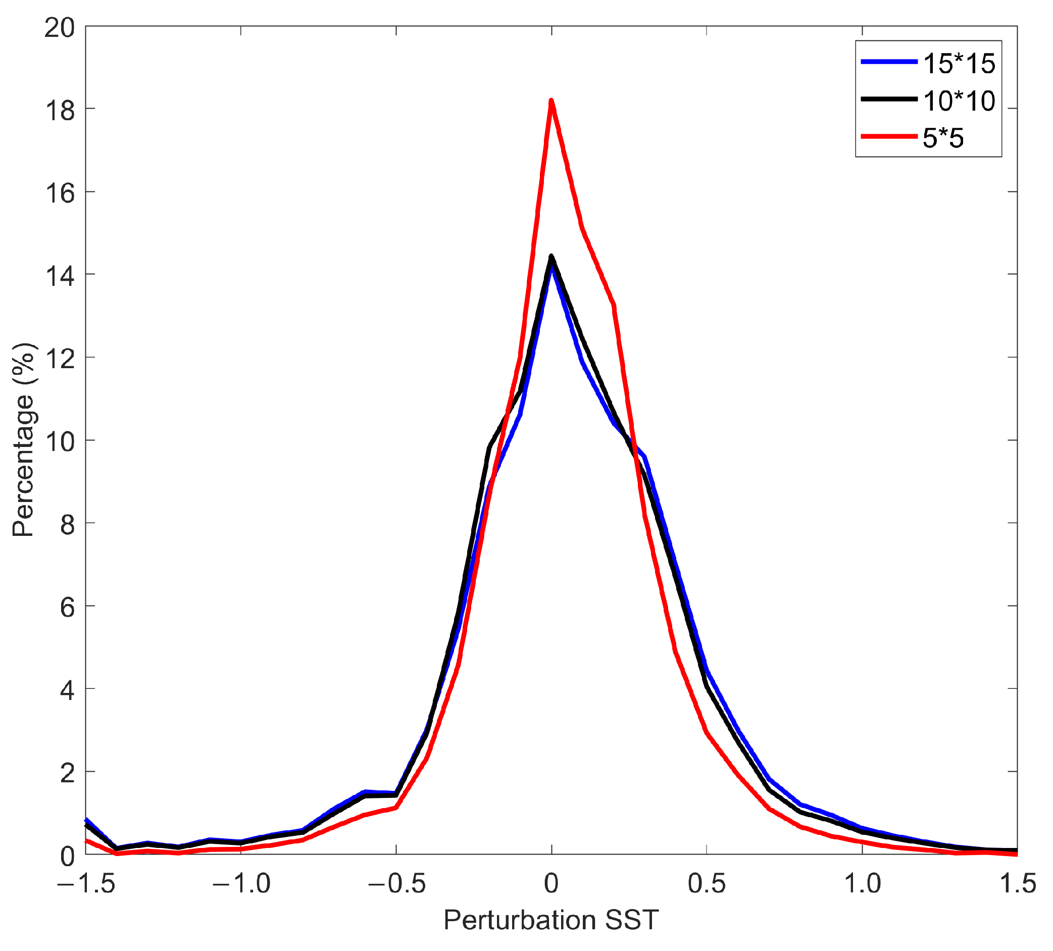
According to the weight function, is the observed value of this point. When reaches the minimum value, the solved is the smooth value at the target point. We selected different half-span parameters for filtering and obtained the probability distribution of the mesoscale signals from 2003 to 2008. When the half-span parameter is 10°, the filtered SST perturbation probability distribution is similar to that obtained when the half-span parameter is greater than 10° (Figure 1).
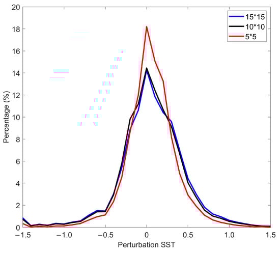
Figure 1.
The probability distributions of the mesoscale magnitude of SST perturbations as a function of the different half-span parameters.
In this study, a half-span parameter of 10° was used to filter and analyze the SST and wind fields in the satellite data to obtain SSTmeso and WSmeso. Then, SSTmeso was used to calculate the along-wind gradient and the cross-wind gradient to obtain ∇down SSTmeso and ∇cross SSTmeso.
The Div(WSmeso) and Curl(WSmeso) were obtained by calculating the divergence and curl of WSmeso.
2.3. Parameterization of Mesoscale Wind Field
The main process of the parameterization scheme was as follows: First, the SSTmeso and WSmeso were obtained from satellite observation data, and the coupling coefficients between Curl(WSmeso) and ∇cross SSTmeso and between Div(WSmeso) and ∇down SSTmeso were calculated, respectively. Then, Div(WSmeso) and Curl(WSmeso) were calculated from the mesoscale SST gradient perturbation based on the resulting coupling coefficient. Finally, the two components of the wind stress perturbation were obtained via a parameterization method.
The focus of the parameterization method was to calculate the WSmeso based on the Div(WSmeso) and Curl(WSmeso). In order to achieve this goal, we chose the Tikhonov regularization method [42,43,44,45].
The wind stress divergence and curl are expressed as follows:
where Ψ and χ represent the stream function and potential function. The discrete form of the above equations is , where and are two components of the wind stress perturbation. A is a difference matrix, and its structure is related to the selected difference scheme. The least squares regression method is generally used to solve this kind of problem, and the solution is
where is the transpose matrix of . For a finite irregular region, A can be ill-conditioned or nonsingular, resulting in instability of the solution [46]. Such ill-posed problems can be effectively solved by the Tikhonov regularization method. According to the Tikhonov regularization method, this problem is equivalent to finding the approximate solution of , where Г is called the Tikhonov matrix, Г is expressed as α I, where α is the regularization coefficient, and 1 × 10⁻⁶ was taken in this paper [47]. I is the unit matrix. The form of this solution is
We developed a new empirical model to study the feedback effect of mesoscale air–sea coupling. This model calculated the disturbance in the SST gradient from the SST perturbation and then calculated the perturbation in wind stress. The model was then nested into the ocean model.
2.4. Ocean Model
We utilized the Regional Ocean Modeling System (ROMS) version 3.4 as the ocean model. The ROMS is a numerical model that operates in three dimensions, accounting for the free surface and following the terrain [48,49]. ROMS provides a variety of mixed parameterization schemes. The harmonic mixing scheme is used in the horizontal mixing in this study, and the Mellor/Yamada Level-2.5 closed parameterization scheme is used in the vertical mixing. The vertical advection adopts the fourth-order central discrete scheme. The tracer and momentum advection in the horizontal direction adopts the third-order upstream discrete scheme.
To mitigate the impact of boundary effects on the simulation of the study region, the model domain encompassed the northwest Pacific, spanning from 20° N to 42° N and from 117° E to 135° E. The horizontal grid resolution was set at 1/8° × 1/8° cos Φ (where Φ represents the latitude). In the vertical direction, the model employed 30 levels (s-coordinates), with increased resolution near the surface and bottom [49,50]. The bathymetry was derived from the Global 2 min Gridded Topographic Data ETOPO2. The time step utilized for the two-dimensional barotropic equations was 30 s, while for the three-dimensional baroclinic equations, it was 300 s.
The European Centre for Medium-Range Weather Forecasts Reanalysis-Interim (ERA-Interim) monthly mean surface wind fields from 1985 to 2015 were utilized as input data to drive the model. The air–sea fluxes were computed using bulk formulae based on atmospheric variables obtained from the National Center for Environmental Prediction (NCEP) reanalysis product spanning the period from 1985 to 2015. These variables include monthly mean longwave radiation, shortwave radiation, atmospheric relative humidity, rainfall, sea surface pressure, and air temperature. The model was set to adjust the temperature by calculating the upward longwave radiation based on the magnitude of the sea surface temperature. The model did not take into account the influence of tides but incorporated the effect of runoff. The initial and boundary conditions for the model were provided by the Simple Ocean Data Assimilation (SODA) 3.4.2 dataset. The calculation of the wind stress in the model used the relative velocity of the wind speed and the flow velocity. All the driving field data were processed into monthly climatology data.
2.5. Sensitivity Experiments
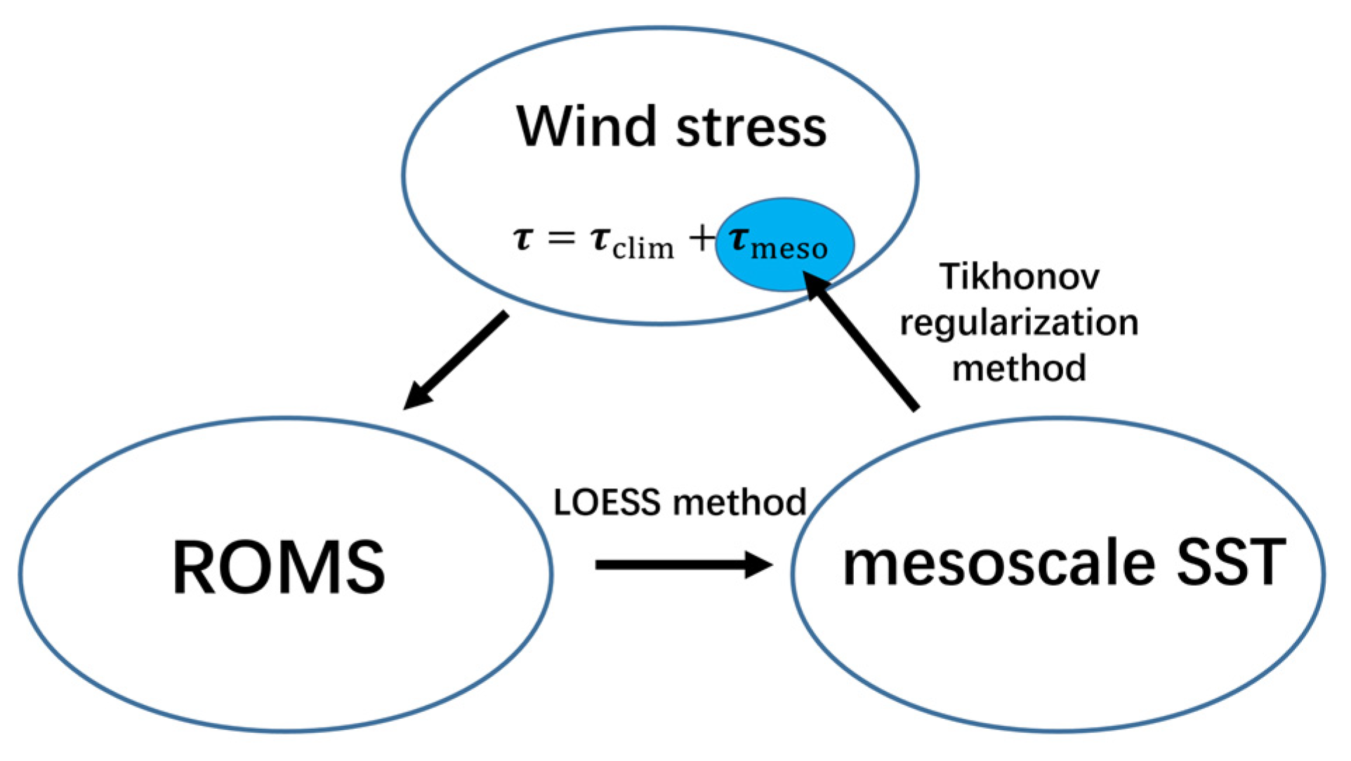
The mode uses the configuration introduced in Section 2.4 and forced by the climatological monthly forced field for 20 years in order to achieve a stable climate state. To study the influence of mesoscale air–sea coupling, two experiments were designed. The first experiment, referred to as the control experiment (CONTROL-E), maintained the same configuration as the previous 20 years. The second experiment was a mesoscale air–sea coupling experiment (MESO-E). In this experiment, the SSTmeso was extracted from the SST at each time step in the model. WSmeso was then obtained using the constructed mesoscale wind field feedback parameterization method described in Section 2.3. This perturbation was superimposed on the climatological wind stress to jointly drive the model. Thus, the ocean model incorporated the mesoscale air–sea coupling process (Figure 2). All experiments were run from the 21st year to the 30th year, and then the feedback effect of mesoscale air–sea coupling on the ocean was analyzed by comparing the 10-year averaged monthly results of the experiment with those of CONTROL-E.

Figure 2.
The flow chart of mesoscale wind field calculation in MESO-E.
3. Results
3.1. Characteristics of Mesoscale SST–Wind Coupling in Observation
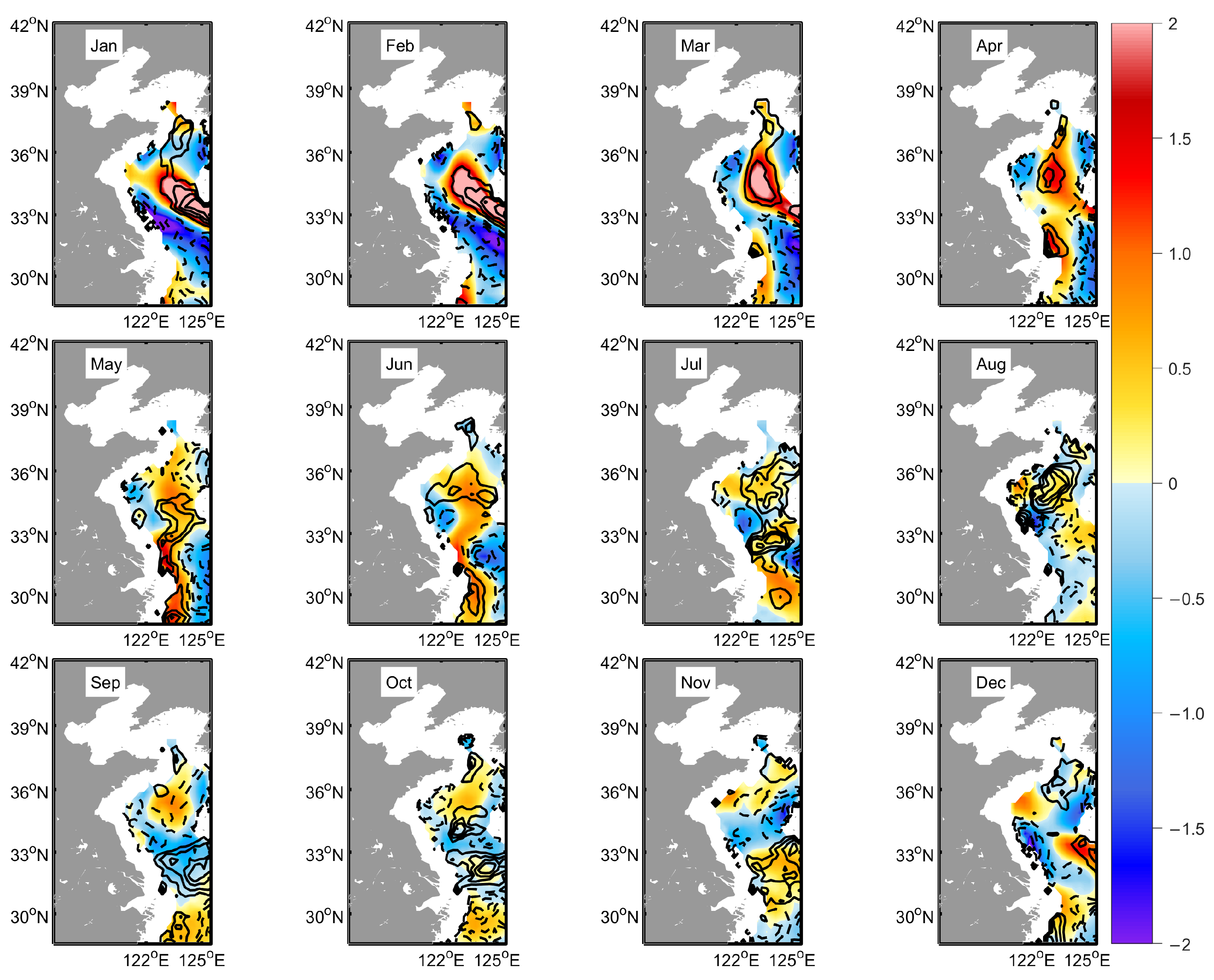
Figure 3 shows the mesoscale air–sea signals extracted from AMSR-E SST data and Quik-SCAT wind field data in 2006. Due to the interference of land electromagnetic waves, some satellite data in offshore waters are default values. The results show that there is a strong mesoscale coupling in the YS and ECS, and the mesoscale SST and wind field show a good positive correlation. At the same time, it can be seen that the mesoscale signal intensity is relatively strong from January to March but relatively weak from September to October.

Figure 3.
Spatially high-pass filtered WSmeso (contours) and SSTmeso (colors) in the different months in 2006. The contour interval is 0.003 N·m−2. The zero contours are not included.
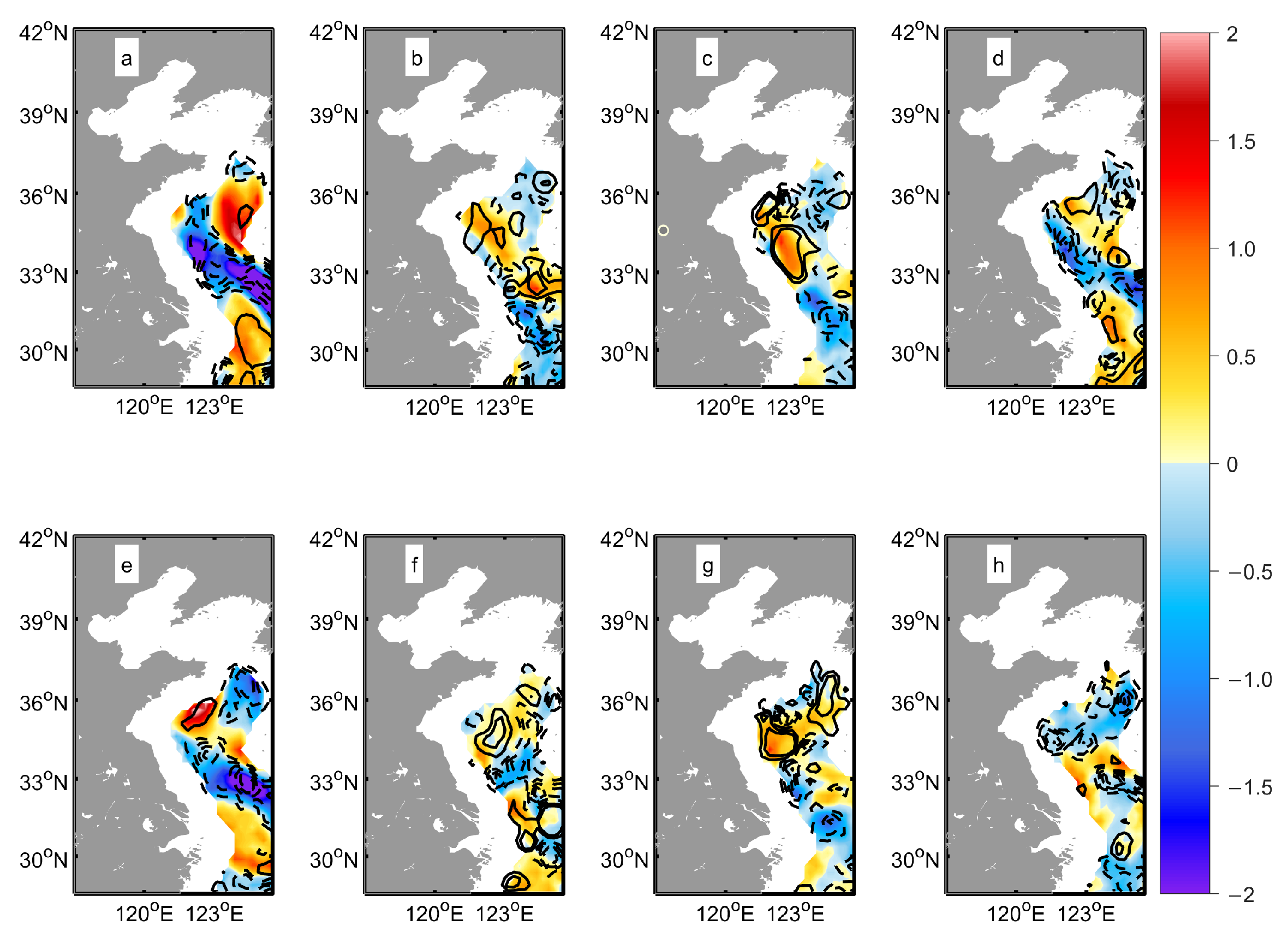
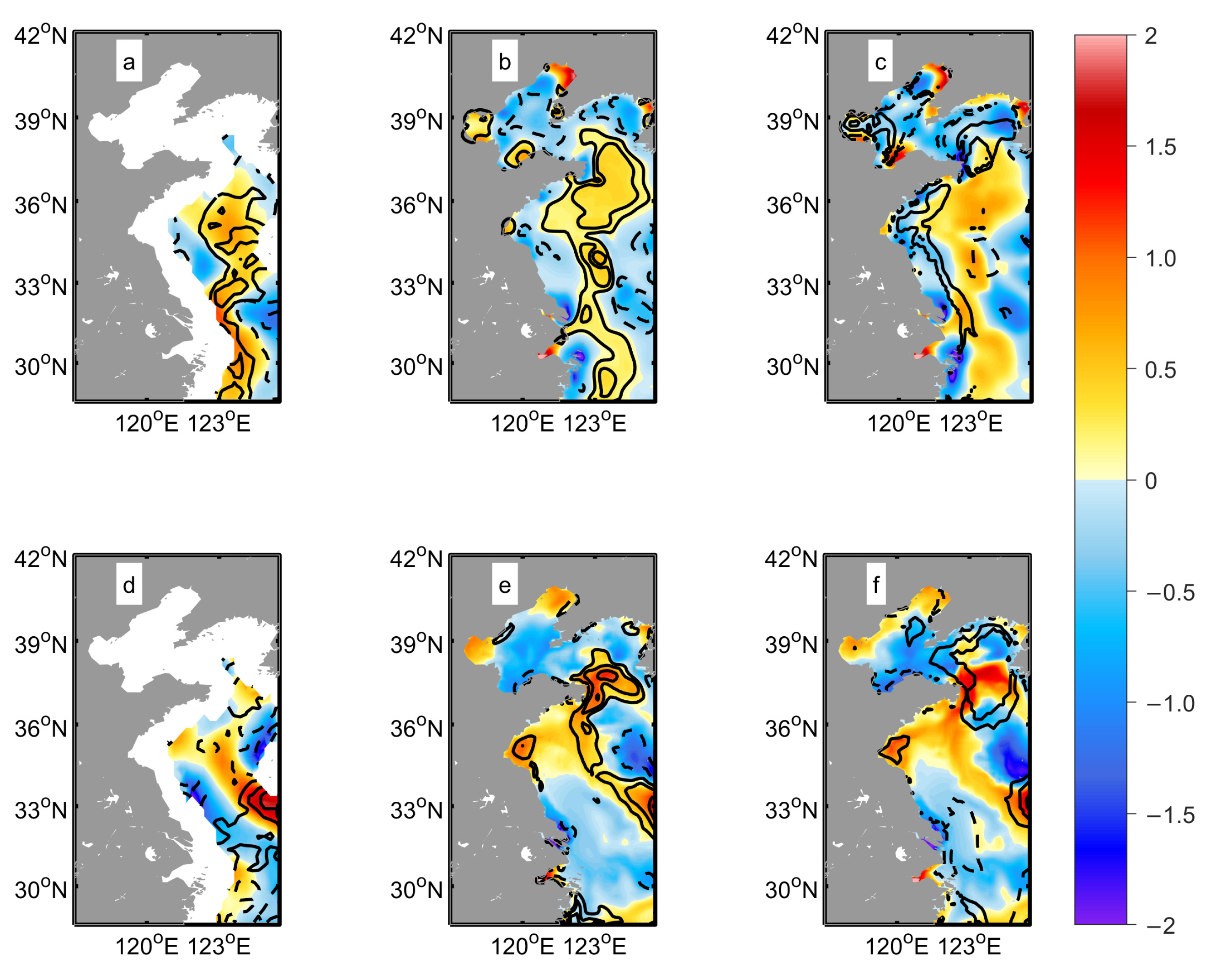
The spatial distributions of the AMSR-E ∇down SSTmeso (∇cross SSTmeso) and Quik-SCAT Div(WSmeso) (Curl(WSmeso)) perturbations in February, June, August, and December 2006 are presented in Figure 4. Spatially, the Div(WSmeso) (Curl(WSmeso)) positively correlated with ∇down SSTmeso (∇cross SSTmeso). The SSTmeso gradient field exhibited both positive and negative values and was widely distributed throughout the YS and ECS.

Figure 4.
Spatially high-pass filtered (upper panel) Div(WSmeso) (contours) and ∇down SSTmeso (colors), and (lower panel) Curl(WSmeso) (contours) and ∇cross SSTmeso (colors) in (a,e) February, (b,f) June, (c,g) August, and (d,h) December 2006. The contour interval is 0.3 N·m−2 per 10,000 km. The zero contours are not included.
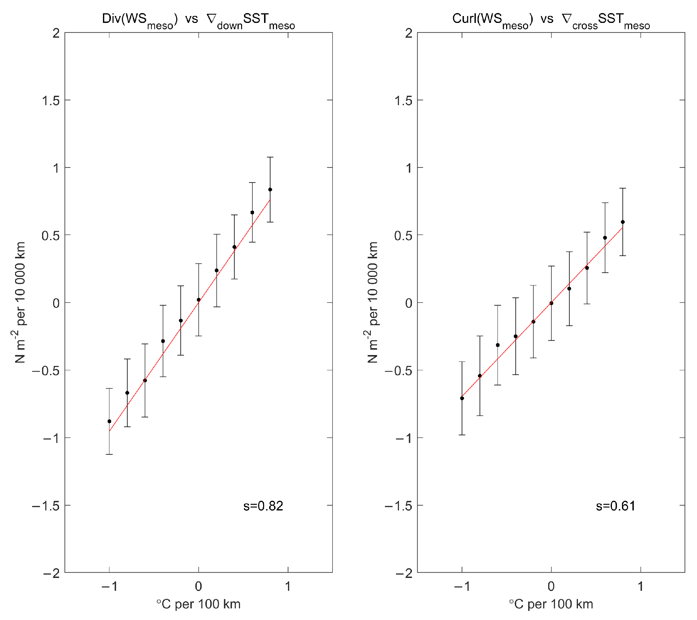
To statistically analyze the correlation between the SSTmeso gradient field and Div(WSmeso) and Curl(WSmeso), Figure 5 displays scatterplots of the magnitudes of Div(WSmeso) and Curl(WSmeso) categorized by the ranges of ∇down SSTmeso and ∇cross SSTmeso, respectively. The coupling coefficients were derived from daily data spanning the period 2003–2008. In Figure 5, the coupling coefficient, denoted as , is represented in scientific notation. The results demonstrated a linear relationship between the mesoscale SST gradient and wind stress divergence and curl perturbations. The coupling coefficient between ∇down SSTmeso and Div(WSmeso) was approximately 0.82 N·m−2/(°C·100 km). The coupling coefficient between ∇cross SSTmeso and Curl(WSmeso) was approximately 0.61 N·m−2/(°C·100 km). This also implied that Div(WSmeso) and Curl(WSmeso) could be derived from ∇down SSTmeso and ∇cross SSTmeso, respectively.
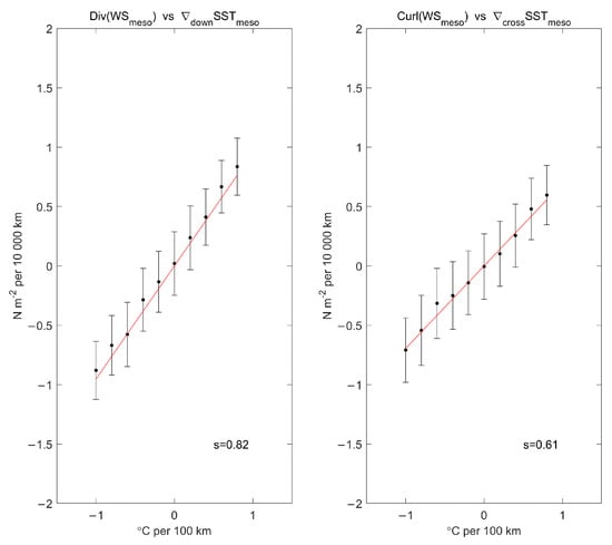
Figure 5.
Scatterplots of the spatially high-pass filtered Quik-SCAT Div(WSmeso) and Curl(WSmeso) binned by ranges of AMSR-E ∇down SSTmeso and ∇cross SSTmeso perturbations. The coupling coefficient is denoted as S. Points and error bars represent the mean and standard deviation in each bin, respectively.
The monthly coupling coefficients between Div(WSmeso) (Curl(WSmeso)) and ∇down SSTmeso (∇cross SSTmeso) were also calculated from daily data spanning the period 2003–2008 (Figure 6). Both coupling coefficients had a persistent pattern of seasonal variation, with relatively high coupling coefficients occurring in summer and relatively low coupling coefficients in October.
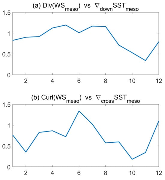
Figure 6.
The monthly variations in the coupling coefficient (N·m−2/(°C·100 km)) between (a) Div(WSmeso) and ∇down SSTmeso and (b) Curl(WSmeso) and ∇cross SSTmeso.
3.2. Simulated Mesoscale SST–Wind Coupling and Its Influence
3.2.1. Simulated Mesoscale SST–Wind Coupling Characteristics
After obtaining the observed monthly averaged mesoscale coupling coefficient between the Div(WSmeso) (Curl(WSmeso)) and ∇down SSTmeso (∇cross SSTmeso), we used the method mentioned in Section 2.3 to construct the mesoscale reconstruction model and applied it to the ROMS model.
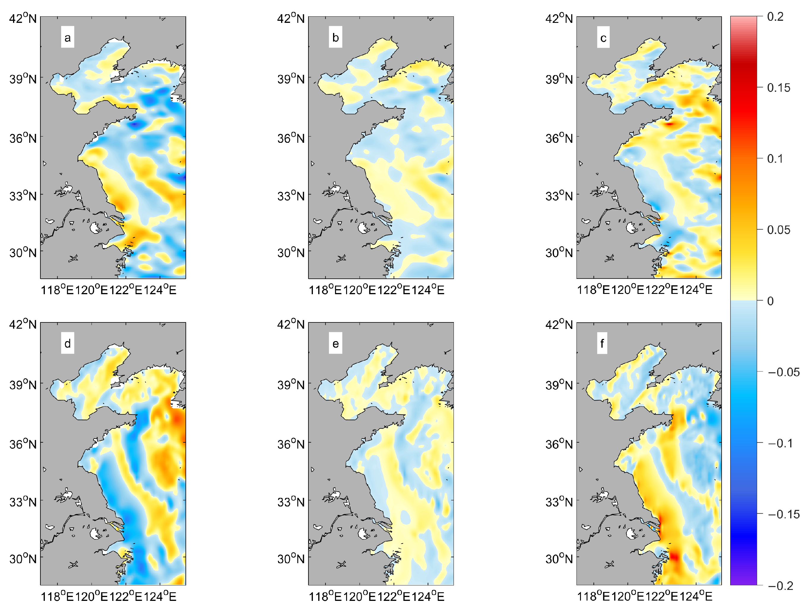
Figure 7a,d show the observed SSTmeso and WSmeso in the summer and winter from the AMSR-E and Quik-SCAT of 2006. Both results showed that the SSTmeso and WSmeso changed seasonally. Moreover, both the observations and simulated outputs of the MESO-E revealed that there were several regions with high positive SSTmeso values in the YS. The spatial distribution of the WSmeso closely corresponded to that of the SSTmeso. These results also indicated that the simulated output of MESO-E successfully captured the spatial and temporal features of SSTmeso and WSmeso observed in the region and their relationships. It is worth noting that the distribution of mesoscale coupling varied between summer and autumn in different years; thus, caution should be taken when using the data solely from 2006 as a reference. However, in CONTROL-E, there is almost no correlation between the distribution characteristics of SSTmeso and WSmeso. This is because, in CONTROL-E, the driving wind field is the climatological monthly mean wind field, which has smoothed the mesoscale signal.
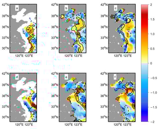
Figure 7.
The SSTmeso (colors) and WSmeso (contours) obtained from (a) observation, (b) MESO-E, and (c) CONTROL-E in summer; the SSTmeso (colors) and WSmeso (contours) obtained from (d) observation, (e) MESO-E, and (f) CONTROL-E in winter. The observations are from AMSR-E and Quik-SCAT data in 2006; the simulated results are from 10-year averaged outputs of MESO-E and CONTROL-E. The contour interval is 0.006 N·m−2. The zero contours are omitted.
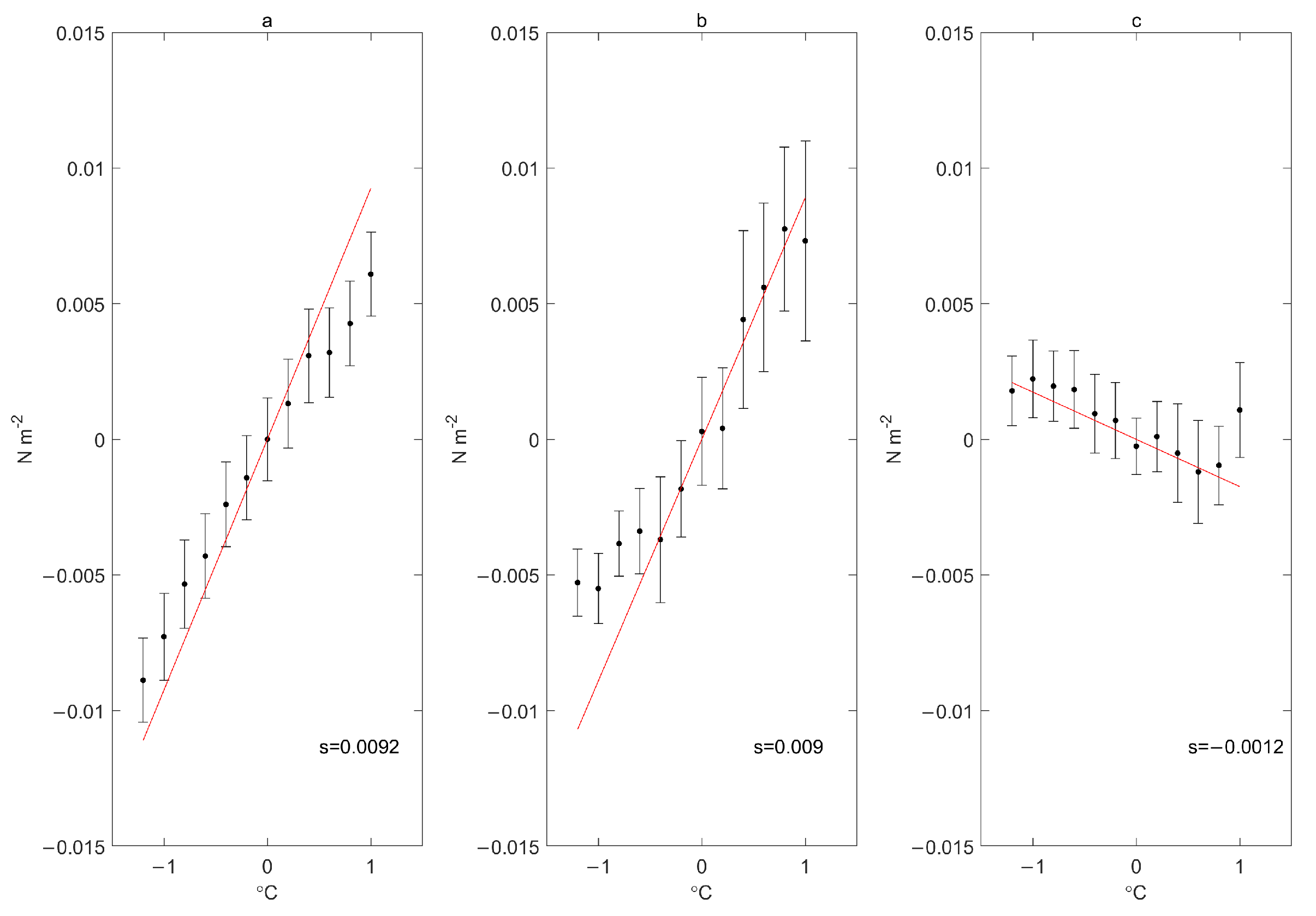
In addition, it can also be seen from the statistical coupling coefficient that CONTROL-E cannot characterize the mesoscale coupling phenomenon at all. The coupling coefficient between SSTmeso and WSmeso was calculated from the output of MESO-E. For the convenience of comparison, we only count the valid regional data on satellite data when processing the data. The simulated coupling coefficient was 0.009 °C/N·m−2, which was nearly identical to the observed value of 0.0092 °C/N·m−2 (Figure 8).
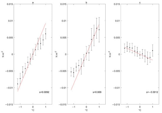
Figure 8.
The (a) 6-year averaged coupling coefficient between Quik-SCAT WSmeso and AMSR-E SSTmeso, (b) 10-year averaged coupling coefficient between WSmeso and SSTmeso from the MESO-E output, and (c) 10-year averaged coupling coefficient between WSmeso and SSTmeso from the CONTROL-E output. Points and error bars represent the mean and standard deviation in each bin, respectively.
3.2.2. The Feedback Effect on the Sea Temperature
These findings suggested that WSmeso could be effectively represented by SSTmeso using the mesoscale wind field empirical model derived from Tikhonov’s regularization method. Then, we used the method and model described in Section 2 to study the effect of the mesoscale SST–wind coupling on dynamic processes in YS and ECS.
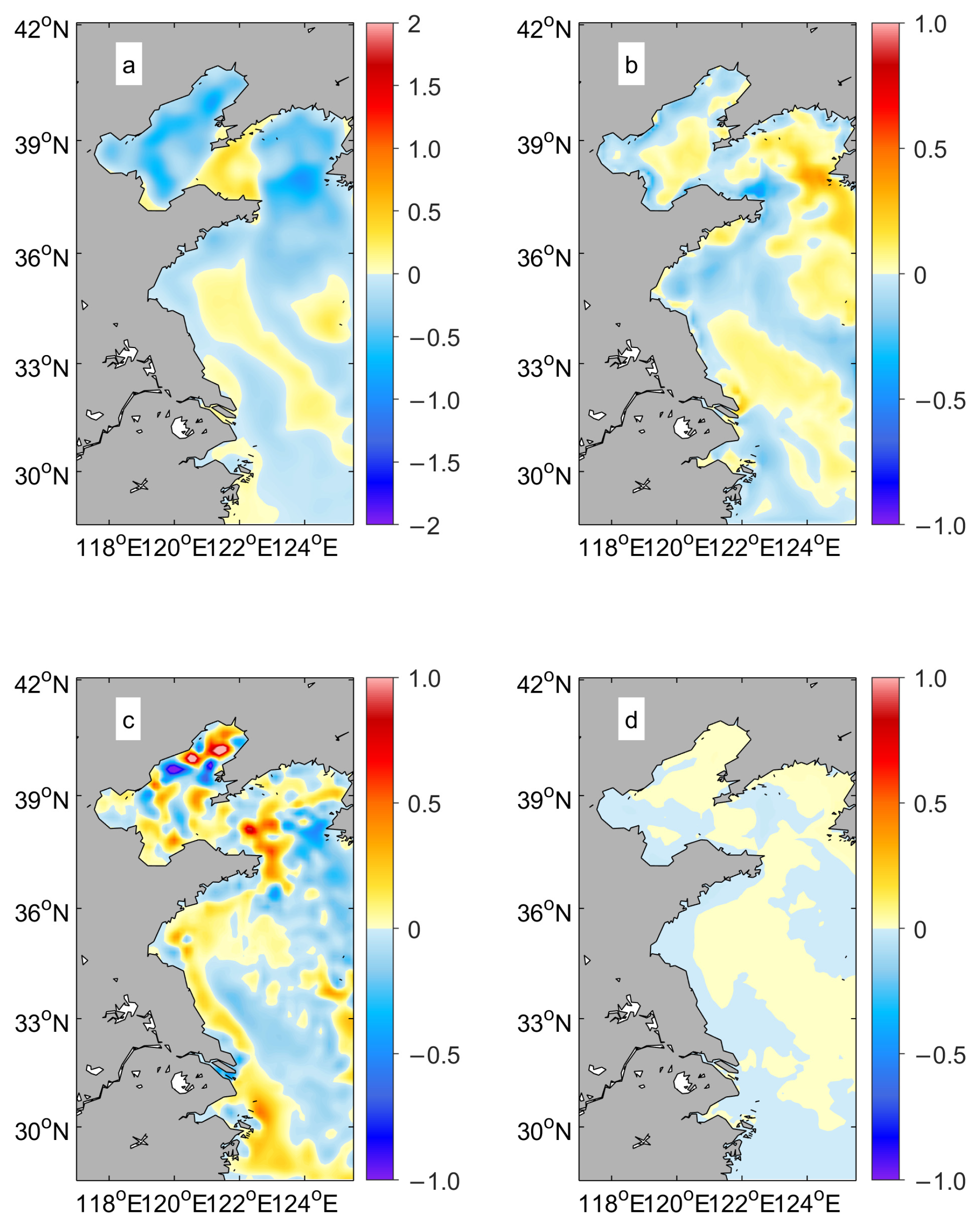
Figure 7a shows the average temperature difference in the upper 50 m of the ocean (MESO-E minus CONTROL-E). The temperature in the nearshore region of the ECS experienced an increase in the MESO-E, with maximum SST values reaching 0.62 °C. In contrast, the temperature in the upper 50 m in most areas of the YS exhibited a decreasing trend throughout the year.
The heat budget analysis in the upper 50 m of the ocean was introduced to investigate the physical mechanisms responsible for the changes in SST under the influence of mesoscale SST–wind coupling. The SST change is controlled by the following heat budget equation:
where means averaged from the upper 50 m, and means the horizontal velocity. The first term on the right-hand side is the horizontal advection. The second and third terms represent the contributions of the net surface heat flux and vertical heat diffusion, respectively. represents the downward net surface heat flux, while represents the diffusive heat flux, and RES represents other remnants that affect the ocean heat budget.
Figure 9 presents the 10-year averaged difference (MESO-E minus CONTROL-E) in the sea temperature and heat budget terms. According to the statistics, the spatial mean values of surface heat flux, horizontal advection, and the vertical diffusion term are approximately 0.0042, −0.0056, and 0.000247 °C/month, respectively. The major factors responsible for the SST difference are horizontal advection and surface heat flux. Horizontal advection tends to increase the sea temperature in the coastal region, aligning with the sea temperature differences caused by the mesoscale coupling (Figure 9a,b). In contrast, the net surface heat flux counteracts the sea temperature difference and mainly suppresses the sea temperature difference induced by horizontal advection (Figure 9a,c). Although the contributions of vertical heat diffusion and the residual (RES) terms are relatively small, they lead to a decrease in sea temperature in the coastal area and an increase in sea temperature in the offshore region (Figure 9a,d).
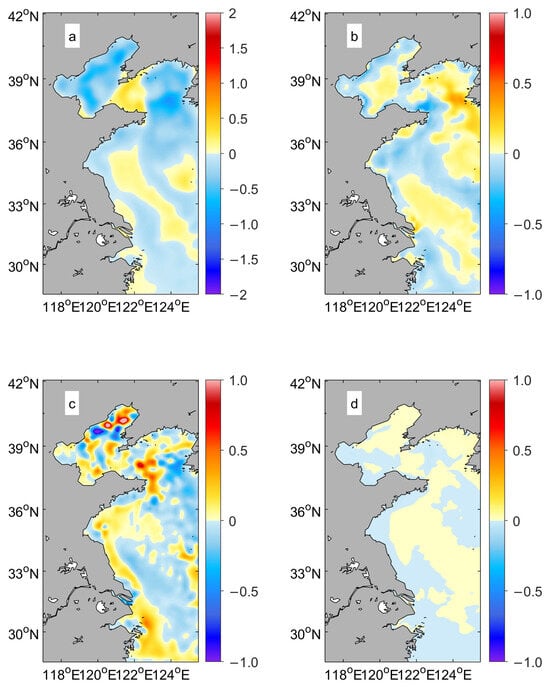
Figure 9.
The 10-year averaged differences (MESO-E minus CONTROL-E) in (a) sea temperature, (b) surface heat flux, (c) horizontal advection, and (d) vertical diffusion in the upper 50 m. The units are °C in (a) and °C/month in (b–d).
3.2.3. The Feedback Effect on Horizontal and Vertical Currents
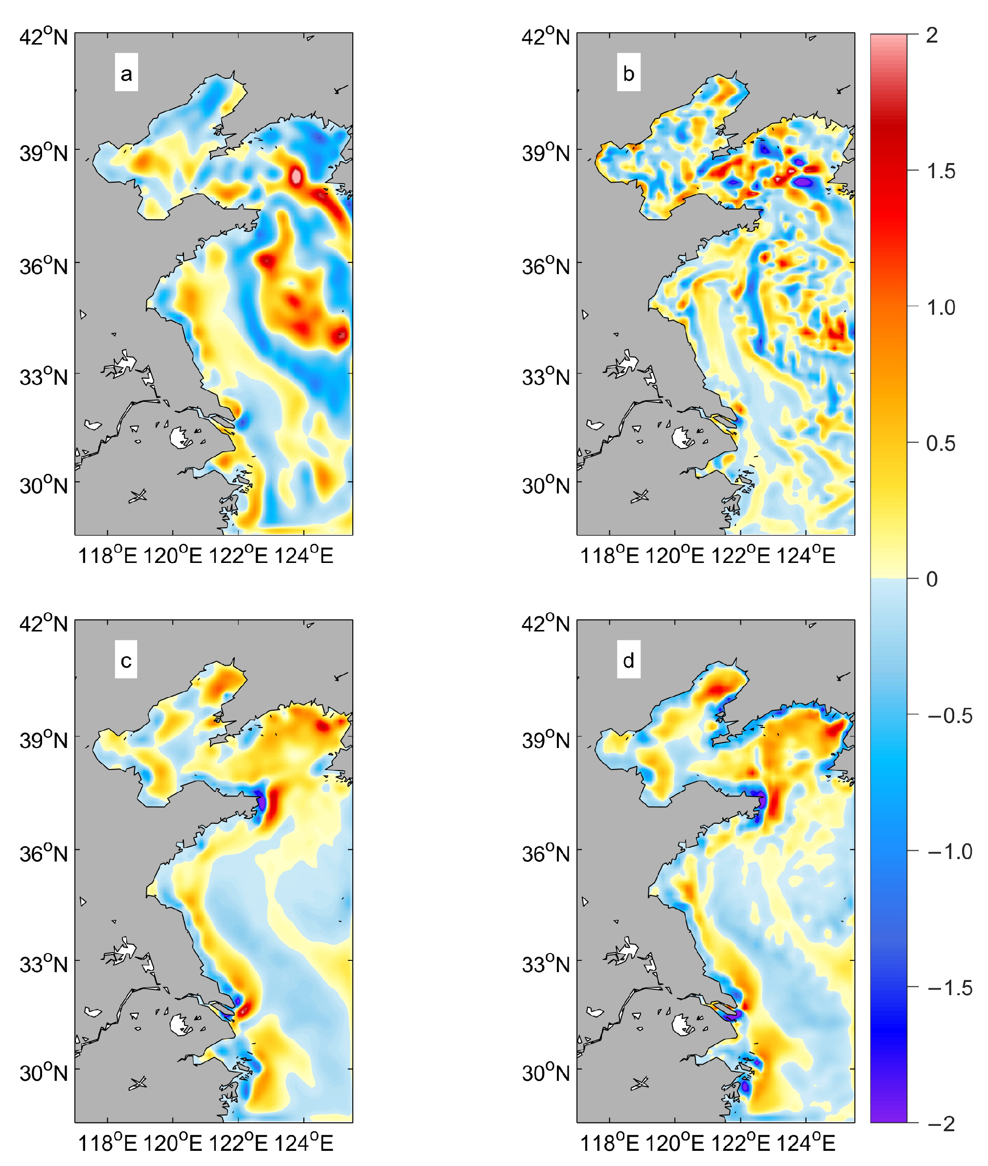
Figure 10 shows the differences in the winter horizontal current between the SODA and CONTROL-E, between MESO-E and CONTROL-E, and between MESO-E and SODA. It shows that the simulated zonal current in CONTROL-E was smaller than that in SODA in the coastal area of the YS and ECS and the middle region of the YS (Figure 10a). The simulated meridional current in CONTROL-E was larger than that in SODA in the nearshore area and the middle area of the YS and smaller than that in SODA in other regions (Figure 10d). After adding the mesoscale coupling method to the model, the simulated zonal current strengthened in the coastal area of the YS and ECS and the middle region of the YS (Figure 10b). The simulated meridional currents weakened in the nearshore area and the middle area of the YS and strengthened in other regions (Figure 10e). In conclusion, the change in ocean horizontal velocity caused by mesoscale coupling can reduce the difference between the model and SODA data well (Figure 10c,f). The strong spatial correlation of the sets of the difference results indicated that the addition of mesoscale ocean–air coupling in winter could significantly improve the simulation accuracy of the horizontal current. Observations showed that in addition to stable positive SSTmeso in the coastal waters of the ECS, the distribution of mesoscale signals in other regions varied significantly in the summer of each year. Therefore, the improvement in the model’s dynamic system was not as pronounced in summer as in winter.

Figure 10.
The 10-year average (a–c) zonal and (d–f) meridional current differences (m/s) in winter between the SODA3.4.2 2011–2020 data and CONTROL-E (SODA minus CONTROL-E, left panel); between MESO-E and CONTROL-E (MESO-E minus CONTROL-E, middle panel), and between MESO-E and SODA (MESO-E minus SODA, right panel). The zonal and meridional current was calculated by averaging vertically up to a depth of 50 m.
As shown in Figure 11, incorporating the mesoscale SST–wind coupling in the model simulation led to a noticeable increase in the upward vertical velocity both in summer and in winter in the nearshore area, especially around the Changjiang Estuary. The introduction of mesoscale air–sea coupling enhanced upwelling in the nearshore area of the ECS by approximately 7% in winter and 16% in summer. Compared with that in CONTROL-E, the Curl(WSmeso) in MESO-E also increased in the nearshore area, showing a spatial variation pattern similar to that of the vertical velocity (Figure 11a,c).
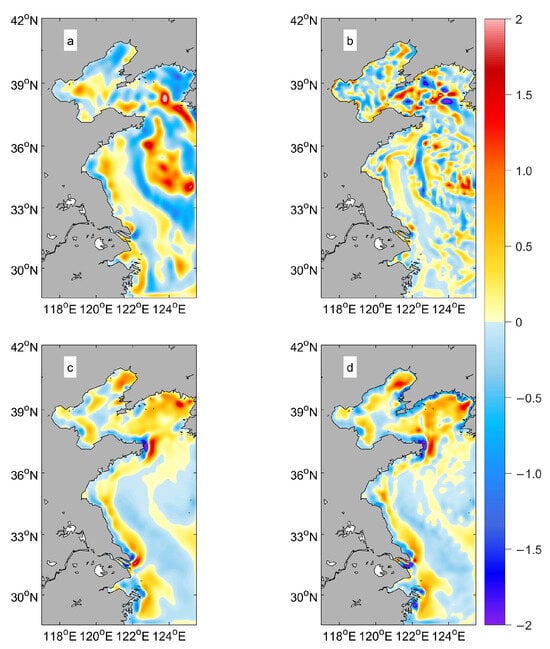
Figure 11.
Differences in the 10-year average (left panel) Curl(WSmeso) (1 × 10⁻⁶ N/m3) and (right panel) vertical current (1 × 10⁻⁷ m/s) in (a,b) winter and (c,d) summer between MESO-E and CONTROL-E (MESO-E minus CONTROL-E). The vertical current was calculated by averaging vertically up to a depth of 50 m.
3.2.4. The Feedback Effect on Eddy Kinetic Energy (EKE)
The 10-year average differences in the budget term of the EKE between MESO-E and CONTROL-E were also calculated (Figure 12b–d). We used the method developed by Renault et al. [51] to calculate the budget of EKE. Based on their analysis, all variables were decomposed into their time means estimated over a 10-year period, denoted by an overbar (─), and their deviations from this mean were indicated using primes (′). Then, the EKE is defined by
where is the density of seawater. The EKE budgets are given by:
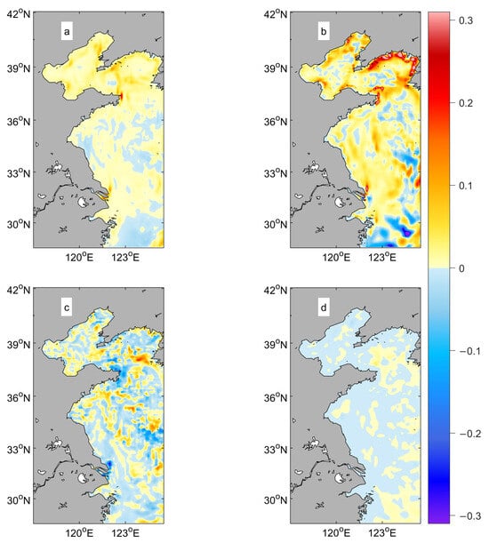
Figure 12.
The 10-year averaged difference in (a) EKE, (b) eddy wind work, and (c) baroclinic conversion from eddy available potential energy to EKE. (d) Conversion between mean kinetic energy and EKE between MESO-E and CONTROL-E (MESO-E minus CONTROL-E). The units are cm3/s3 in (a,b,c) and 1 × 10⁻² cm3/s3 in (d).
On the right-hand side, the first term corresponds to the eddy wind work; the second term represents the baroclinic conversion between eddy available potential energy and EKE; and the third term represents the barotropic conversion between mean kinetic energy and EKE. is the energy dissipation term. is the three-dimensional velocity vector.
Figure 12a illustrates the 10-year average difference in EKE between MESO-E and CONTROL-E. The results showed that the addition of mesoscale air–sea coupling enhanced the EKE in most regions of the YS and the northern region of the ECS. The estimated enhancement was approximately 17%. The eddy wind work term and baroclinic conversion term were important in the EKE change. Compared with that in the CONTROL-E, the eddy wind work term in the MESO-E increased in most regions of the YS and the northern region of the ECS (Figure 12b). However, the baroclinic conversion term decreased in most of the study area (Figure 12c). The change in the barotropic conversion term was two orders of magnitude smaller than that in the eddy wind work and baroclinic conversion terms (Figure 12d).
4. Discussion and Conclusions
The LOESS method effectively separated the mesoscale signals from the satellite data fields (Figure 3 and Figure 4). Observations revealed a positive correlation between Div(WSmeso) (Curl(WSmeso)) and ∇down SSTmeso (∇cross SSTmeso). The mesoscale coupling strength is stronger in spring and summer.
The empirical model of mesoscale SST–wind coupling derived from Tikhonov’s regularization method was well applied to the ROMS model and successfully reproduced the observed coupling of SSTmeso and WSmeso (Figure 7 and Figure 8). WSmeso could be effectively represented by SSTmeso using the empirical model. These methods provided a suitable way to study the mesoscale SST–wind coupling and its effect on the dynamic environment in the YS and ECS.
The simulated results revealed that incorporating the mesoscale SST–wind coupling results in significant changes in sea temperature in the YS and ECS. The sea temperature in the offshore region of the ECS exhibits a noticeable increase, with maximum sea temperature changes reaching 0.62 °C. The sea temperature in most areas of the YS decreases throughout the year, effectively mitigating the SST error introduced by the climate model in this region [39]. The heat budget analysis indicated that the major factors contributing to the difference in sea temperature were surface heat flux and horizontal advection. Horizontal advection tends to increase the sea temperature in the nearshore area, while surface heat flux acts to dampen the sea temperature difference. In general, the changes in sea temperature resulting from mesoscale air–sea interactions are primarily driven by changes in heat flux due to changes in wind speed and the horizontal advection effect.
The more realistic horizontal and vertical velocity outputs from MESO-E also indicated that incorporating the mesoscale air–sea coupling empirical model into the climatological model can reduce errors and improve our modeling capabilities in this region (Figure 10 and Figure 11). After incorporating mesoscale air–sea coupling, the horizontal current velocity is more realistic, and it is found that the upward vertical velocity is significantly enhanced in the nearshore area. The introduction of mesoscale air–sea coupling enhances upwelling in the nearshore area of the ECS by approximately 7% in winter and 16% in summer. A comparison of the vertical velocity difference with the wind stress curl difference suggests that the change in Ekman pumping, which is triggered by the curl of WSmeso, is the primary factor that induces the change in the vertical velocity. The EKE is also influenced by mesoscale air–sea coupling. The estimated EKE enhancement is approximately 17% in the YS. The EKE budget analysis revealed that the increase in the EKE under the influence of mesoscale air–sea coupling is primarily attributed to the change in the eddy wind work.
These findings were consistent with previous research. For instance, studies on marine heat waves in the YS and ECS have shown that the occurrence of marine heat waves is largely influenced by decreased wind speeds and the advection of warm water [52,53]. Marine heat waves have an important influence on marine ecosystems [54]. Moreover, the SST in winter is associated with the YS cold water mass, which provides a suitable environment for primary production and benthic organisms [55,56]. Therefore, investigating the influence of mesoscale air–sea interactions on SST is essential for understanding the changes in both dynamic and ecological environments in the YS and ECS.
The changes in current and EKE are mainly caused by the wind field variation induced by mesoscale air–sea coupling. The primary reason for the improvement in the horizontal current is the influence of mesoscale wind fields. For example, in the coastal waters of the YS, there is a strong positive SSTmeso, which can enhance the local East Asian monsoon and subsequently strengthen the southward flow. The variation in vertical velocity aligns with that in Curl(WSmeso) within the nearshore area (Figure 11), suggesting that the difference in Ekman pumping, which is triggered by the wind stress curl, is the primary factor inducing the change in vertical velocity. Researchers have found that the curl of WSmeso can modulate Ekman pumping, particularly in areas with intense mesoscale eddy activities [29,35]. The 10-year average differences in each term in the EKE budgets between MESO-E and CONTROL-E indicate that the addition of mesoscale air–sea coupling enhances the EKE in the YS. This enhancement is primarily attributed to the change in the wind field caused by mesoscale air–sea coupling, which increases the energy input to the eddy. The conversion from eddy available potential energy to EKE works to dampen the EKE change in the nearshore sea area. The difference in conversion between the mean kinetic energy and EKE is relatively small.
Upwelling is an important nutrient source for the growth of phytoplankton in the nearshore area of the ECS [57]. Mesoscale motion is also critical in the distribution of nutrients and phytoplankton [58,59]. Therefore, the study of the vertical velocity and EKE changes associated with mesoscale air–sea coupling is also essential for understanding the ecological environment in the YS and ECS.
This paper provides insight into the underlying physical processes involved in the feedback effect of mesoscale SST–wind coupling and contributes to the enhancement of model simulations. These results have important implications for understanding the possible responses of the ecosystem to mesoscale air–sea coupling in the YS and ECS.
Author Contributions
Conceptualization, C.C. and L.X.; Methodology, C.C. and L.X.; Software, C.C.; Validation, C.C.; Formal analysis, C.C.; Investigation, C.C.; Resources, C.C.; Data curation, C.C.; Writing—original draft preparation, C.C. and L.X.; Writing and editing, C.C. and L.X.; Visualization, C.C.; Supervision, C.C.; Project administration, C.C.; Funding acquisition, C.C. and L.X. All authors have read and agreed to the published version of the manuscript.
Funding
This study was supported by the National Natural Science Foundation of China (NSFC) (Nos. 42206001 and 42206011), Shandong Provincial Natural Science Foundation (ZR2021QD081 and ZR2021QD160), and the basic research foundation (2023PY004, 2023JBZ02 and 2023RCKY046) in Qilu University of Technology, as well as the Youth Innovation Technology Project of Higher School in Shandong Province (No. 2023KJ326).
Data Availability Statement
All the satellite data are obtained from the Asia-Pacific Data-Research Center (APDRC) of the University of Hawaii, which is available at http://apdrc.soest.hawaii.edu/las/v6/dataset?catitem = 1 (accessed on 3 February 2023). The model results are made available in the repository of Mendeley Data https://data.mendeley.com/datasets/sjdh5yxmt2/1 (accessed on 5 June 2024).
Conflicts of Interest
The authors declare no conflicts of interest.
References
- Bourras, D.; Reverdin, G.; Giordani, H.; Caniaux, G. Response of the atmospheric boundary layer to a mesoscale oceanic eddy in the northeast Atlantic. J. Geophys. Res. 2004, 109, 18114. [Google Scholar] [CrossRef]
- Castelao, R.M. Sea Surface Temperature and Wind Stress Curl Variability near a Cape. J. Phys. Oceanogr. 2012, 42, 2073–2087. [Google Scholar] [CrossRef]
- Chelton, D.B.; Esbensen, S.K.; Schlax, M.G.; Schopf, P.S. Observations of Coupling between Surface Wind Stress and Sea Surface Temperature in the Eastern Tropical Pacific. J. Clim. 2001, 14, 1479–1498. [Google Scholar] [CrossRef]
- Chelton, D.B.; Schlax, M.G.; Samelson, R.M. Summertime Coupling between Sea Surface Temperature and Wind Stress in the California Current System. J. Phys. Oceanogr. 2007, 37, 495–517. [Google Scholar] [CrossRef]
- Chow, C.H.; Liu, Q. Eddy effects on sea surface temperature and sea surface wind in the continental slope region of the northern South China Sea. Geophys. Res. Lett. 2012, 39, 2601. [Google Scholar] [CrossRef]
- Giordani, H.; Planton, S.; Benech, B.; Kwon, B. Atmospheric boundary layer response to sea surface temperatures during the SEMAPHORE experiment. J. Geophys. Res. 1998, 103, 25047–25060. [Google Scholar] [CrossRef]
- Minobe, S.; Kuwano-Yoshida, A.; Komori, N.; Xie, S.P.; Small, R.J. Influence of the Gulf Stream on the troposphere. Nature 2008, 452, 206–209. [Google Scholar] [CrossRef]
- O’ Neill, L.W.; Chelton, D.B.; Esbensen, S.K. The Effects of SST-Induced Surface Wind Speed and Direction Gradients on Midlatitude Surface Vorticity and Divergence. J. Clim. 2010, 23, 255–281. [Google Scholar] [CrossRef]
- O’ Neill, L.W.; Chelton, D.B.; Esbensen, S.K. Covariability of Surface Wind and Stress Responses to Sea Surface Temperature Fronts. J. Clim. 2012, 25, 5916–5942. [Google Scholar] [CrossRef]
- O’ Neill, L.W.; Chelton, D.B.; Esbensen, S.K.; Wentz, F.J. High-Resolution Satellite Measurements of the Atmospheric Boundary Layer Response to SST Variations along the Agulhas Return Current. J. Clim. 2005, 18, 2706–2723. [Google Scholar] [CrossRef]
- Sweet, W.; Fett, R.; Kerling, J.; La Violette, P. Air-sea interaction effects in the lower troposphere across the north wall of the Gulf Stream. Mon. Weather Rev. 1981, 109, 1042–1052. [Google Scholar] [CrossRef]
- Seo, H.; O’ Neill, L.W.; Bourassa, M.A.; Czaja, A.; Drushka, K.; Edson, J.B.; Fox-Kemper, B.; Frenger, I.; Gille, S.T.; Kirtman, B.P.; et al. Ocean Mesoscale and Frontal-Scale Ocean–Atmosphere Interactions and Influence on Large-Scale Climate: A Review. J. Clim. 2023, 36, 1981–2013. [Google Scholar] [CrossRef]
- Chelton, D.B.; Xie, S. Coupled Ocean-Atmosphere Interaction at Oceanic Mesoscales. Oceanography 2010, 23, 52–69. [Google Scholar] [CrossRef]
- Byrne, D.; Münnich, M.; Frenger, I.; Gruber, N. Mesoscale atmosphere ocean coupling enhances the transfer of wind energy into the ocean. Nat. Commun. 2016, 7, ncomms11867. [Google Scholar] [CrossRef]
- Byrne, D.; Papritz, L.; Frenger, I.; Münnich, M.; Gruber, N. Atmospheric Response to Mesoscale Sea Surface Temperature Anomalies: Assessment of Mechanisms and Coupling Strength in a High-Resolution Coupled Model over the South Atlantic. J. Atmos. Sci. 2015, 72, 1872–1890. [Google Scholar] [CrossRef]
- Jing, Z.; Wang, S.; Wu, L.; Chang, P.; Zhang, Q.; Sun, B.; Ma, X.; Qiu, B.; Small, J.; Jin, F.F.; et al. Maintenance of mid-latitude oceanic fronts by mesoscale eddies. Sci. Adv. 2020, 6, eaba7880. [Google Scholar] [CrossRef]
- Nakamura, H.; Sampe, T.; Tanimoto, Y.; Shimpo, A. Observed associations among storm tracks, jet streams and midlatitude oceanic fronts. Geophys. Monogr. Ser. 2004, 147, 329–345. [Google Scholar] [CrossRef]
- Putrasahan, D.A.; Miller, A.J.; Seo, H. Regional coupled ocean–atmosphere downscaling in the Southeast Pacific: Impacts on upwelling, mesoscale air–sea fluxes, and ocean eddies. Ocean. Dyn. 2013, 63, 463–488. [Google Scholar] [CrossRef]
- Xu, G.; Chang, P.; Ma, X.; Li, M. Suppression of winter heavy precipitation in Southeastern China by the Kuroshio warm current. Clim. Dyn. 2019, 53, 2437–2450. [Google Scholar] [CrossRef]
- Frenger, I.; Gruber, N.; Knutti, R.; Münnich, M. Imprint of Southern Ocean eddies on winds, clouds and rainfall. Nat. Geosci. 2013, 6, 608–612. [Google Scholar] [CrossRef]
- Desbiolles, F.; Blamey, R.; Illig, S.; James, R.; Barimalala, R.; Renault, L.; Reason, C. Upscaling impact of wind/sea surface temperature mesoscale interactions on southern Africa austral summer climate. Int. J. Climatol. 2018, 38, 4651–4660. [Google Scholar] [CrossRef]
- Piazza, M.; Terray, L.; Boé, J.; Maisonnave, E.; Sanchez-Gomez, E. Influence of small-scale North Atlantic sea surface temperature patterns on the marine boundary layer and free troposphere: A study using the atmospheric ARPEGE model. Clim. Dyn. 2016, 46, 1699–1717. [Google Scholar] [CrossRef]
- Renault, L.; Hall, A.; McWilliams, J.C. Orographic shaping of US West Coast wind profiles during the upwelling season. Clim. Dyn. 2016, 46, 273–289. [Google Scholar] [CrossRef]
- Bane, J.M.; Osgood, K.E. Wintertime air-sea interaction processes across the Gulf Stream. J. Geophys. Res. Ocean. 1989, 94, 10755. [Google Scholar] [CrossRef]
- Bunker, A.F.; Worthington, L.V. Energy Exchange Charts of the North Atlantic Ocean. Bull. Am. Meteorol. Soc. 1976, 57, 670–678. [Google Scholar] [CrossRef]
- Wei, Y.; Kang, X.; Pei, Y. A case study of the consistency problem in the inverse estimation. Acta Oceanol. Sin. 2017, 36, 45–51. [Google Scholar] [CrossRef]
- Wei, Y.; Wang, H.; Zhang, R. Mesoscale wind stress-SST coupled perturbations in the Kuroshio Extension. Prog. Oceanogr. 2019, 172, 108–123. [Google Scholar] [CrossRef]
- Ma, X.; Jing, Z.; Chang, P.; Liu, X.; Montuoro, R.; Small, R.J.; Bryan, F.O.; Greatbatch, R.J.; Brandt, P.; Wu, D.; et al. Western boundary currents regulated by interaction between ocean eddies and the atmosphere. Nature 2016, 535, 533–537. [Google Scholar] [CrossRef]
- Gaube, P.; Chelton, D.B.; Samelson, R.M.; Schlax, M.G.; O’Neill, L.W. Satellite Observations of Mesoscale Eddy-Induced Ekman Pumping. J. Phys. Oceanogr. 2015, 45, 104–132. [Google Scholar] [CrossRef]
- Albert, A.; Echevin, V.; Lévy, M.; Aumont, O. Impact of nearshore wind stress curl on coastal circulation and primary productivity in the Peru upwelling system. J. Geophys. Res. 2010, 115, 12033. [Google Scholar] [CrossRef]
- Bakun, A.; Nelson, C.S. The Seasonal Cycle of Wind-Stress Curl in Subtropical Eastern Boundary Current Regions. J. Phys. Oceanogr. 1991, 21, 1815–1834. [Google Scholar] [CrossRef]
- Seo, H.; Miller, A.J.; Norris, J.R. Eddy–Wind Interaction in the California Current System: Dynamics and Impacts. J. Phys. Oceanogr. 2016, 46, 439–459. [Google Scholar] [CrossRef]
- Vecchi, G.A.; Xie, S.P.; Fischer, A.S. Ocean-Atmosphere Covariability in the Western Arabian Sea. J. Clim. 2004, 17, 1213–1224. [Google Scholar] [CrossRef]
- Ratheesh, S.; Chaudhary, A.; Bhowmick, S.A.; Agarwal, N. Monsoonal Variability in the Mesoscale Coupling of Wind and SST in the Arabian Sea. Pure Appl. Geophys. 2022, 179, 385–398. [Google Scholar] [CrossRef]
- Seo, H. Distinct Influence of Air–Sea Interactions Mediated by Mesoscale Sea Surface Temperature and Surface Current in the Arabian Sea. J. Clim. 2017, 30, 8061–8080. [Google Scholar] [CrossRef]
- Bryan, F.O.; Tomas, R.; Dennis, J.M.; Chelton, D.B.; Loeb, N.G.; McClean, J.L. Frontal Scale Air-Sea Interaction in High-Resolution Coupled Climate Models. J. Clim. 2010, 23, 6277–6291. [Google Scholar] [CrossRef]
- Song, Q.T.; Chelton, D.B.; Esbensen, S.K.; Thum, N.; O’Neill, L.W. Coupling between Sea Surface Temperature and Low-Level Winds in Mesoscale Numerical Models. J. Clim. 2009, 22, 146–164. [Google Scholar] [CrossRef]
- Perlin, N.; de Szoeke, S.P.; Chelton, D.B.; Samelson, R.M.; Skyllingstad, E.D.; O’Neill, L.W. Modeling the Atmospheric Boundary Layer Wind Response to Mesoscale Sea Surface Temperature Perturbations. Mon. Weather. Rev. 2014, 142, 4284–4307. [Google Scholar] [CrossRef]
- Balaguru, K.; Van Roekel, L.P.; Leung, L.R.; Veneziani, M. Subtropical Eastern North Pacific SST Bias in Earth System Models. J. Geophys. Res. Ocean. 2021, 126, e2021JC017359. [Google Scholar] [CrossRef]
- Shan, H.X.; Dong, C.M. The SST–Wind Coupling Pattern in the East China Sea Based on a Regional Coupled Ocean–Atmosphere Model. Atmosphere-Ocean 2017, 55, 230–246. [Google Scholar] [CrossRef]
- Cleveland, W.S.; Devlin, S.J. Locally Weighted Regression: An Approach to Regression Analysis by Local Fitting. J. Am. Stat. Assoc. 1988, 83, 596–610. [Google Scholar] [CrossRef]
- Cui, C.; Zhang, R.; Wang, H.; Wei, Y. Representing surface wind stress response to mesoscale SST perturbations in western coast of South America using Tikhonov regularization method. J. Oceanol. Limnol. 2020, 38, 679–694. [Google Scholar] [CrossRef]
- Cui, C.; Zhang, R.; Wei, Y.; Wang, H. Mesoscale wind stress-SST coupling induced feedback to the ocean in the western coast of South America. J. Oceanol. Limnol. 2021, 39, 785–799. [Google Scholar] [CrossRef]
- Jin, X.; Dong, C.; Kurian, J.; McWilliams, J.C.; Chelton, D.B.; Li, Z. SST–Wind Interaction in Coastal Upwelling: Oceanic Simulation with Empirical Coupling. J. Phys. Oceanogr. 2009, 39, 2957–2970. [Google Scholar] [CrossRef]
- Wei, Y.; Zhang, R.; Wang, H. Mesoscale wind stress–SST coupling in the Kuroshio extension and its effect on the ocean. J. Oceanogr. 2017, 73, 785–798. [Google Scholar] [CrossRef]
- Foxkemper, B.; Ferrari, R.; Pedlosky, J. On the Indeterminacy of Rotational and Divergent Eddy Fluxes. J. Phys. Oceanogr. 1959, 33, 478–483. [Google Scholar] [CrossRef]
- Li, Z.; Chao, Y.; McWilliams, J.C. Computation of the Streamfunction and Velocity Potential for Limited and Irregular Domains. Mon. Weather. Rev. 2006, 134, 3384–3394. [Google Scholar] [CrossRef]
- Shchepetkin, A.F.; McWilliams, J.C. The regional oceanic modeling system (ROMS): A split-explicit, free-surface, topography-following-coordinate oceanic model. Ocean. Model. 2005, 9, 347–404. [Google Scholar] [CrossRef]
- Song, Y.; Haidvogel, D. A Semi-implicit Ocean Circulation Model Using a Generalized Topography-Following Coordinate System. J. Comput. Phys. 1994, 115, 228–244. [Google Scholar] [CrossRef]
- Haidvogel, D.B.; Arango, H.; Budgell, W.P.; Cornuelle, B.D.; Curchitser, E.; Di Lorenzo, E.; Fennel, K.; Geyer, W.R.; Hermann, A.J.; Lanerolle, L.; et al. Ocean forecasting in terrain-following coordinates: Formulation and skill assessment of the Regional Ocean Modeling System. J. Comput. Phys. 2008, 227, 3595–3624. [Google Scholar] [CrossRef]
- Renault, L.; Molemaker, M.J.; McWilliams, J.C.; Shchepetkin, A.F.; Chelton, D.; Illig, S.; Hall, A. Modulation of Wind Work by Oceanic Current Interaction with the Atmosphere. J. Phys. Oceanogr. 2016, 46, 1685–1704. [Google Scholar] [CrossRef]
- Cai, R.; Tan, H.; Kontoyiannis, H. Robust Surface Warming in Offshore China Seas and Its Relationship to the East Asian Monsoon Wind Field and Ocean Forcing on Interdecadal Time Scales. J. Clim. 2017, 30, 8987–9005. [Google Scholar] [CrossRef]
- Gao, G.; Marin, M.; Feng, M.; Yin, B.; Yang, D.; Feng, X.; Ding, Y.; Song, D. Drivers of Marine Heatwaves in the East China Sea and the South Yellow Sea in Three Consecutive Summers During 2016–2018. J. Geophys. Res. Ocean. 2020, 125, e2020JC016518. [Google Scholar] [CrossRef]
- Smale, D.A.; Wernberg, T.; Oliver, E.C.J.; Thomsen, M.; Harvey, B.P.; Straub, S.C.; Burrows, M.T.; Alexander, L.V.; Benthuysen, J.A.; Donat, M.G.; et al. Marine heatwaves threaten global biodiversity and the provision of ecosystem services. Nat. Clim. Chang. 2019, 9, 306–312. [Google Scholar] [CrossRef]
- Tan, S.C.; Shi, G.Y. The relationship between satellite-derived primary production and vertical mixing and atmospheric inputs in the Yellow Sea cold water mass. Cont. Shelf Res. 2012, 48, 138–145. [Google Scholar] [CrossRef]
- Zhang, J.; Xu, F.; Liu, R. Community structure changes of macrobenthos in the South Yellow Sea. Chin. J. Oceanol. Limnol. 2012, 30, 248–255. [Google Scholar] [CrossRef]
- Tseng, Y.-F.; Lin, J.; Dai, M.; Kao, S.-J. Joint effect of freshwater plume and coastal upwelling on phytoplankton growth off the Changjiang River. Biogeosciences 2014, 11, 409–423. [Google Scholar] [CrossRef]
- Mahadevan, A. The Impact of Submesoscale Physics on Primary Productivity of Plankton. Annu. Rev. Mar. Sci. 2016, 8, 161–184. [Google Scholar] [CrossRef]
- Ruiz, S.; Claret, M.; Pascual, A.; Olita, A.; Troupin, C.; Capet, A.; Tovar-Sánchez, A.; Allen, J.; Poulain, P.; Tintoré, J.; et al. Effects of oceanic mesoscale and submesoscale frontal processes on the vertical transport of phytoplankton. J. Geophys. Res. Ocean. 2019, 124, 5999–6014. [Google Scholar] [CrossRef]


Disclaimer/Publisher’s Note: The statements, opinions and data contained in all publications are solely those of the individual author(s) and contributor(s) and not of MDPI and/or the editor(s). MDPI and/or the editor(s) disclaim responsibility for any injury to people or property resulting from any ideas, methods, instructions or products referred to in the content. |
© 2024 by the authors. Licensee MDPI, Basel, Switzerland. This article is an open access article distributed under the terms and conditions of the Creative Commons Attribution (CC BY) license (https://creativecommons.org/licenses/by/4.0/).