Abstract
Maritime transport is the most widely used means of transporting goods, and forecasts indicate that it will continue to grow in the coming years, which is why the IMO is regulating energy efficiency and emissions from maritime transport with exhaustive monitoring. The most widely used measure of energy efficiency during operation on a ship is the Energy Efficiency Operational Indicator (EEOI); however, the difficulty in obtaining references for this indicator, together with the great variability that exists between shipowners when choosing terms such as “cargo transported”, among others, means that this operational indicator of energy efficiency in ships does not have the expected results. This work develops a two-phase procedure for the selection of representative EEOI values for ships, taking into account parameters such as ship speed, cargo, mode of operation and the subsequent determination of a suitable control system that allows the continuous and real-time implementation of measures to improve energy and environmental efficiency on the ship. The proposed final procedure is effective in terms of improving energy efficiency and emissions, on top of being simple, easily implementable, working in real time and adapting to navigation circumstances while keeping emissions under control.
1. Introduction
Maritime transport carries more than 85% of the world’s goods by volume [1,2]. In the coming years, the transport of goods by sea is expected to grow by more than 2.8%, and the distances travelled is also expected to increase significantly. This growth will continue to increase in the coming years [3]. This has led the IMO to introduce various guidelines to regulate energy efficiency at both the design and operational phases using the Energy Efficiency Design Index (EEDI), the Energy Efficiency Operational Indicator (EEOI), the Ship Energy Efficiency Management Plan (SEEMP), the Energy Efficiency of Existing Ships Index (EEXI) and the Carbon Intensity Indicator (CII) in the decades between 2008 and 2018 [4].
The most widely used measure to evaluate the energy efficiency in ship operations is still the EEOI [5,6], serving as a tool to measure the emission of CO2 into the environment per transport work; it represents the real efficiency per transport in a vessel in operation [7].
The EEOI uses the actual cargo transported over the distances travelled to calculate transport work, effectively taking into account the use of the ship’s capacity [8]. For voyages carried out in ballast condition, the AER (Annual Efficiency Ratio) is used instead as a substitute [9]. Many studies have validated the use of EEOI for both consumption savings and emissions reduction, such as Waleed Tehia et al. (2020), who verified its benefits in container ships [10]. Similarly, Joel R. Perez and Carlos A. Reusser (2020) demonstrated the efficiency of ship technology using the EEOI [11], while Tien Anh Tran (2020) confirmed its benefits in bulk carriers [12]. Berna and Görkem (2021) highlighted its reliability under varying operational circumstances, such as different fuel types, environmental conditions, and distances travelled [13]. Furthermore, Osung EE et al. (2024) showed that the EEOI is suitable for assessing energy efficiency in ship operations, particularly noting emissions reductions at low speeds, and these conclusions were also addressed in other similar studies [14,15,16,17]. Other studies have also shown that real-time monitoring of EEOI provides valuable data for optimizing energy efficiency and ship consumption [18,19,20]. C. Capezza et al. (2019) found statistical models, such as PLS, useful in improving emissions and consumption, although they recognize challenges in implementation [21]. Ailong Fan et al. (2023) emphasized the importance of controlling energy variables to optimize consumption and emissions, noting the difficulties in obtaining real-time results due to the need for extensive databases [22]. Overall, the real-time monitoring of variables like the EEOI can significantly optimize energy efficiency, despite challenges in automating control and optimization processes.
However, some researchers question the effectiveness of the EEOI due to its failure to account for operational variability, climate and mode of operation [9,23,24]. Others, like Shuang Zhang et al. (2019), propose alternative methods for measuring energy efficiency, arguing that the EEOI’s reliance on different indicators for “transport work” leads to inadequate results [25]. Operational variables undermine the EEOI as a tool for technical judgement, as noted by Ghaforian Masodzadeh (2018) and Faber et al. (2009), who argue that it is unsuitable for a mandatory policy and is difficult to compare across vessel types [26,27]. Payman et al. (2022) further critiques the EEOI’s dependence on operating conditions [28].
Furthermore, unlike other energy efficiency indicators like the EEDI or CII, the EEOI lacks reference values [8,29,30,31]. To help resolve this, the IMO’s 2020 report, “Fourth IMO GreenHouse Gas Study”, discusses potential reference values for the EEOI, highlighting the variability in its calculation that may lead to inaccurate emissions data, and suggests that future modifications may be necessary for emissions regulation [32].
The EEOI’s effectiveness is therefore a debated topic to this day. While some authors criticize its limitations, others still consider it the best method for quantifying a ship’s energy efficiency during operation. However, no comprehensive studies have yet been conducted to adapt the EEOI calculation required by the IMO to a more multidisciplinary methodology—one that incorporates environmental variability, operational modes, ship speed and other factors, as suggested in the IMO’s 2020 report.
Recent efforts have aimed to make EEOI calculations more representative of transport conditions, but further studies are needed to account for navigational factors. Perera and Mo (2016) suggested that big data could improve energy efficiency indicators, reducing CO2, SOx and NOx emissions [33]. Kim et al. (2020) pointed out the need to study the EEOI’s dependence on navigational conditions [34], while Zhang et al. (2021) proposed alternative models to address EEOI variability and optimize emissions [35], and Chen et al. (2023) emphasized the importance of studying speed and the ship type’s impact on the EEOI [36].
This year, studies continued to highlight the need for a multidisciplinary approach to EEOI calculations, considering navigational conditions. Chen et al. (2024) highlighted the necessity of further research into speed’s effect on the EEOI [15]. Cepowski and Kacprzak (2024) proposed new emission estimation methods, arguing that the EEOI overlooks key navigational factors [37], and Sardar et al. (2024) stressed the importance of refining selection procedures for carbon intensity indicators in future studies [38].
Ensuring that the EEOI calculation procedure can be automated and controlled in real time is the challenge addressed in this study. This article develops a multidisciplinary EEOI calculation procedure that includes the variability of the environment of the ship, navigation conditions, speed and operating modes, thus making its calculation much more accurate as a measure of energy efficiency and emissions control in operation and turning the EEOI into a very useful control measure tool for the SEEMP through real-time EEOI control with systems that facilitate implementation on the ship and do not require large computational needs.
This article is divided into two main parts. The first one develops a procedure that allows the detection of the representative values of the EEOI in the overall navigation and the navigation conditions of a ship in a multidisciplinary way. The second part consists of finding a procedure that allows the effective control of the EEOI and is implementable in the control systems of the ships to optimize the energy efficiency and the emissions in the SEEMP, for each ship, in order to have the most realistic values of emissions and the EEOI and to be able to design effective emission improvement measures.
2. Methodology: Presentation of the Ship and the Cyber-Physical System
As we mentioned in the Introduction, this study aims to find a procedure for calculating the EEOI in real time that takes into account the conditions of the navigation environment that have been shown to have the greatest influence on this indicator, but are not reflected directly in the IMO formula [8]. Once this procedure has been developed and the representative EEOI curves have therefore been obtained, the best statistical control procedure is analyzed so that it not only meets the condition of control effectiveness, but is also easily implementable in the ship’s system, providing information on EEOI deviations in real time that allows for the effective optimization of the ship’s energy efficiency and emissions. To do this, we will work with a real cyber-physical system, with real data from various voyages of a gas tanker that carries a real-time monitoring system for the variables with high influence. We will then develop the system to obtain the most representative values of the EEOI from a multidisciplinary perspective, followed by a study on the statistical control of these representative values to ensure they are implementable and effective. Finally, there will be a Discussion section and a Conclusion section.
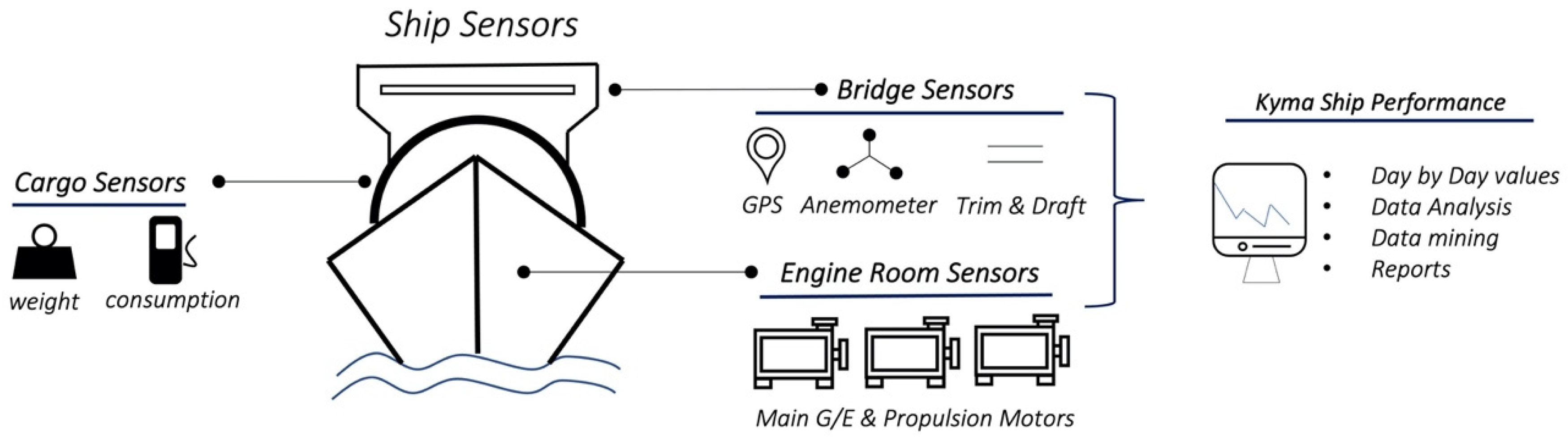
The data used in this study was collected from a typical vessel, representative of the liquefied natural gas (LNG) transport class. The vessel in question has an approximate cargo capacity of 173,400 cubic metres and is equipped with a 42,750 kW dual-fuel electric propulsion plant. The propulsion plant consists of three motor generators of 11,400 kW each and one of 8550 kW, which feed two electric propulsion motors of 13,600 kW each. In addition, the dual-fuel propulsion engines allow operation with both liquefied natural gas (LNG), heavy fuel oil (HFO) and marine diesel oil (MDO), complying with IMO Tier III emission regulations in gas mode and Tier II in liquid fuel mode. The cyber-physical system (CPS) implemented to analyze the propulsion fuel consumption on an LNG vessel integrates advanced sensors, communication infrastructure and specialized software. The sensors are distributed throughout the engine room, bridge and tanks, collecting the information displayed on Table 1.

Table 1.
Types of sensors and their collected information.
The information collected by the sensors is transmitted in real time through a robust communication network and processed by the 2.0 version of the Kyma Ship Performance software [31]. This software analyses the collected data, allowing the real-time monitoring of the engine performance and fuel consumption, and generates detailed reports to optimize the operational efficiency of the vessel. These include variables such as draft, environmental conditions such as wind speed and propulsion system characteristics that influence resistance [32]. The results are presented to the users through intuitive interfaces, facilitating informed decision making and improving the efficiency and sustainability of maritime operations. The data from the reports generated by the software is what has been utilized in this study. Figure 1 shows the configuration of this cyber-physical system.
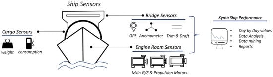
Figure 1.
Configuration of the cyber-physical system of the example ship.
The software used allows the differentiation between fuel consumption intended for propulsion and consumption intended for other services; this capability is essential to be able to clearly discern representative consumption values in transport, thus accurately measuring the analysis of propulsion plant consumption in all operating modes of the vessel and its circumstances.
The process of cleaning and verifying the information obtained from the vessel’s sensors was rigorous, following established methodologies to ensure the validity of the data. This multi-sensory data collection and analysis approach has been validated in previous studies, demonstrating its effectiveness in both modelling and estimating fuel consumption [18,39,40].
3. Block I: Analysis and Detection of the Most Representative EEOI
This section analyses the most representative EEOI of the ship’s transport by selecting values from the database created during the ship’s voyages, both in the condition of navigation with load and in ballast, based on those conditions that have been shown in the literature to have a great influence on the ship’s consumption.
3.1. Inclusion of Load Conditions
An LNG ship, depending on the loading conditions, can make voyages in two types of conditions: cargo and ballast, a distinction that is considered relevant both from the IMO point of view and from the bibliography [13,41,42]. Differentiating between these two types of voyages is very important in the EEOI because the parameter that is considered as “mass transported” varies. In the case of the cargo condition, the mass of the product transported on the vessel is used directly, while in the ballast condition, other calculations are required [5,43,44].
The IMO defines EEOI as the mass of CO2 emissions divided by the workload over a predefined period of time and follows the formula showcased in Equation (1).
As mentioned in the Introduction, this indicator presents the problem that when using the cargo transported by the ship for its calculation, in those voyages that are made with the ship in ballast, the EEOI cannot be calculated. For these cases, the AER (Annual Efficiency Ratio) is used to evaluate the annual operating efficiency of the ship, including the periods in which the ship may be in ballast (without effective cargo). In this case, the DWT (dead weight of the ship) is used as the cargo transported during the whole year. The calculation of AER follows the form showcased in Equation (2).
Both formulas share many variables and are represented below:
In these formulas, the variables are defined as follows:
- is the type of fuel.
- is the mass of fuel consumed in a voyage.
- is the fuel mass to CO2 conversion factor for the fuel .
- is the cargo transported (in tons) or the work performed (number of containers or passengers), or in the case of passenger ships the gross tonnage.
- D is the distance in nautical miles corresponding to the cargo transported or the work performed.
- is the deadweight of the ship.
In our case study, for those voyages carried out with cargo, Equation (1) will be applied, and for those carried out in ballast, Equation (2) will be employed.
3.2. Inclusion of Actual Load Values
In the IMO formulas, the cargo transported on the voyage is included, but in a gas tanker, this cargo varies every day because part of the product is consumed to carry out the transport work. Including the real cargo in the equation makes it necessary to calculate the EEOI or the AER on a daily basis instead of per voyage.
To do this, we will calculate the daily EEOI in the following way: We will subtract the gas cargo consumed by the propulsion of the previous day, since the ship consumed around 99.5% LNG and 0.5% MDO in the period under study. This same criterion will be applied in the calculation of the daily AER for ballast voyages, where the sum of the ship’s DWT and the amount of LNG carried by the ship to feed the propulsion system during the voyage will be used as the transported cargo. This transported cargo, as in cargo voyages, also decreases day by day and therefore the cargo consumed the previous day will also be subtracted from its daily calculation of the AER. In this way, the reality of the ship’s transport efficiency will be reflected.
Therefore, according to the loading condition for real data of transported cargo, the value EEOIdiary will follow the form of Equation (3), and the value AERdiary will follow the form of Equation (4), both of which are showcased below:
In these formulas, the variables are defined as follows:
- : The day that’s being studied
- : Tonnes of MDO equivalent (gas in MDO and MDO formats) consumed on day j.
- : 3206 g CO2/ton MDO.
- : The cargo transported (in tons) at the beginning of the calculation day j in Equation (3), and the gas fuel load for propulsion transported (in tons) at the beginning of the calculation day j in Equation (4).
- : Distance in nautical miles traveled per day j.
- : Ship Deadweight in Tns.
3.3. Inclusion of the Operational Modes
One of the most important variables in the consumption of a ship is the mode of operation, since a ship at anchor or in port does not consume the same amount of energy as when in navigation mode. For the calculation of the EEOI and the AER, it is essential to have data only from the navigation mode, since during loading and unloading and at anchor or in port, no merchandise is transported; therefore, the calculation of the operating energy indicator would not be applicable according to the IMO regulations. In order to include only the navigation mode in the calculation, a representative database must be developed for the calculations of the daily EEOI and the daily AER. In this study, the data were collected during six complete consecutive voyages, three voyages with cargo and three voyages in ballast, in which no major breakdowns occurred that could have altered the energy efficiency of the ship. In this way, the data are guaranteed to be representative of a normal operation of the ship. The duration of the selected voyages was as follows:
- Three voyages with cargo with a duration of 31, 4 and 34 days.
- Three ballast voyages with a direction of 9, 27 and 12 days.
Through the software, the data on consumption, speed and distance travelled were obtained each day of the selected voyages at the same time. In addition to the values, the software facilitated their grouping by navigation conditions and speeds at minimum intervals of 0.1 h (6 min). Of the 2816.2 h of combined total duration of the six voyages, 574 h in which the ship was in port or at anchor have been discarded. Therefore, only those values in which the ship was in navigation mode remain in the database. This step is very important because the percentage of time that the ship consumed without any distance travelled is 20.38%, almost a quarter of the time that it consumed without travelling any distance, which clearly reflects the need to select the data by the ship’s operating mode in order to have representative EEOI and AER calculations.
Another issue to consider in this section is the duration of the navigation. Once only the EEOI and AER values for navigation have been selected, it must be noted that not all trips have the same duration. There are trips where the navigation mode lasts a few hours and others last more than 20 days. Therefore, weighting the EEOI and AER values based on the time to obtain an adequate average EEOI is another step that must be taken.
3.4. Inclusion of the Speed Ranges of the Ship
Ship speed is a fundamental factor in the energy consumption of the ship, as it influences factors such as the relative speed of the wind, the power required by the engines, and the resistance to the ship’s progress. This makes it one of the most common research objectives in the maritime industry, from the search for speed optimization at each point of the voyage to the creation of the practice known as slow steaming to reduce consumption and emissions. Some studies even confirm that 85% of the variability of the EEOI is due to the variability of the vessel’s speed. Because of all these factors, it is important to conduct an exhaustive analysis of this variable when choosing a representative EEOI [45,46].
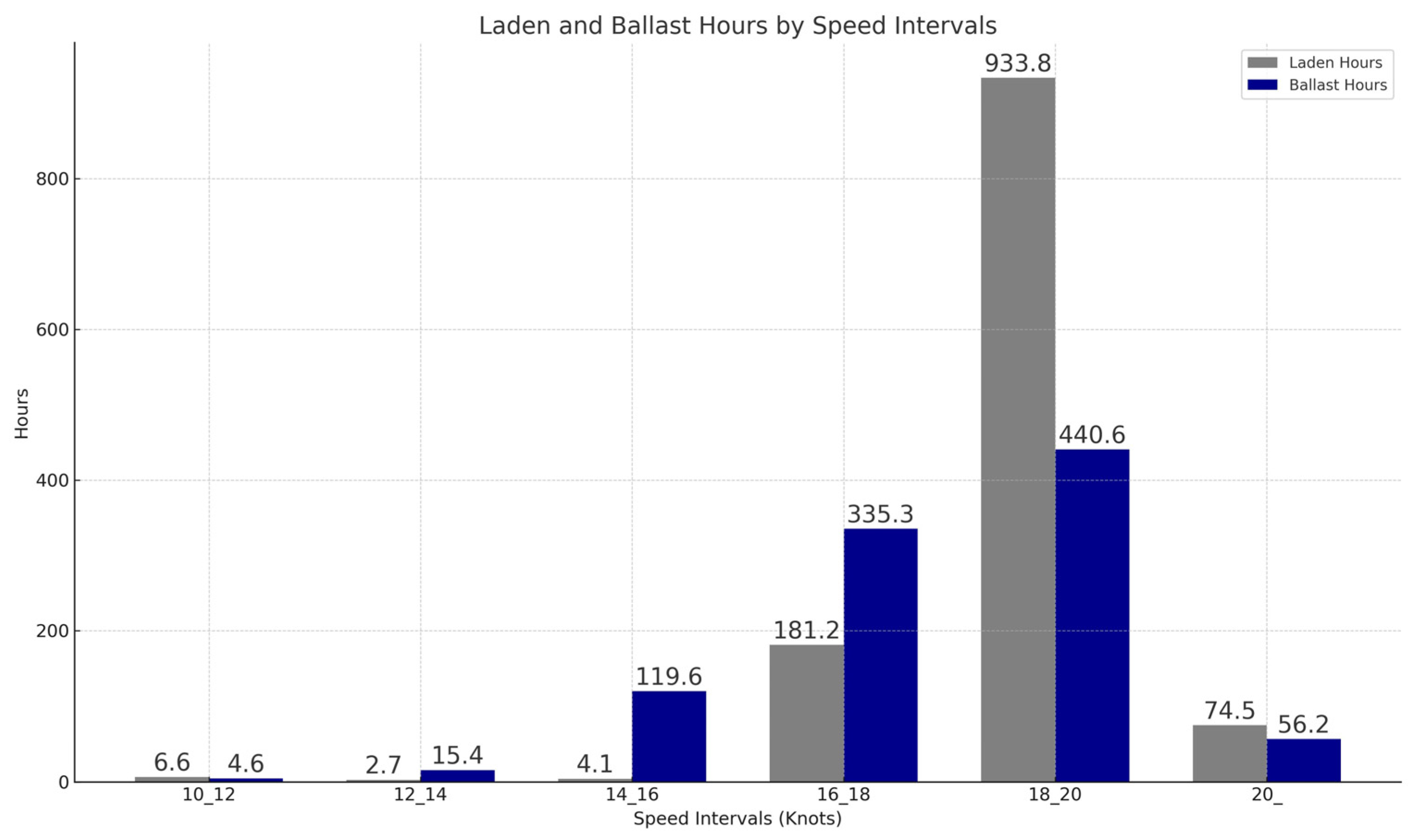
In the database of this study, the daily results of consumption and distances travelled are classified in a series of speed ranges. The range from 0 to 10 knots is considered maneuvering, and from 10 knots, it is considered navigation. Additionally, ranges of 2 knots wide, up to 20 knots, are established. In the last range, all speeds higher than 20 knots are established. These ranges under study and the number of hours that have been conducted in these ranges are shown in Figure 2.

Figure 2.
Graphical representation of the time spent in each range of velocities.
In view of the results of the table and figure above, a concentration of navigation hours around the navigation speed between 18 and 20 knots can be seen. It amounts to 63.2% of the voyage time spent in load and ballast conditions.
To assess the impact of the navigation speed on the EEOI and AER, the average values corresponding to each speed interval in which the ship has operated were calculated. These averages were determined using a weighted mean based on the number of daily hours of occurrence for each speed. The calculation method for the EEOI values is presented in Equation (5), with the same procedure being applicable to the AER values, using their respective parameters.
In these formulas, the variables are defined as follows:
- : Average Energy Efficiency Operational Indicator of the speed interval i.
- : EEOI for speed interval i on day j.
- : Number of daily navigation hours in speed interval i on day j.
- : Total number of daily navigation hours across the speed interval i.
The results obtained are shown in Table 2.
Table 2.
Classification of the mean and standard deviation values of the daily averaged EEOI according to the speed intervals. The most prominent interval is highlighted in color.
After carrying out the grouping and classification techniques of the daily EEOI and AER values, it is noted that by classifying the values by the representative variables of the vessel, the distortion generated in the global data by the mixture of different conditions is progressively eliminated. Therefore, it is considered that this selection, which discriminates between loading conditions (laden and ballast), does not take into account PORT and MANEUVERING conditions, and classifies by speed ranges, is crucial in the study, as the control charts that will be employed in the next block use the mean value (u_0) and the standard deviation (σ) of each data set as parameters. This method ensures that the calculated mean is representative of each speed range, providing a solid and appropriate basis for defining the central line of the control charts.
Furthermore, the method used to calculate the average of the daily EEOI and AER, weighted by the number of daily hours of occurrence, improves the accuracy of the mean calculation, eliminating the possibility of distortion by extreme or infrequent values. Thus, the mean values and standard deviations in Table 2 are set as representative bases, providing the most representative values of the ship’s navigation mode and its deviations. This provides clear limits for what is considered normal and facilitates the identification of values outside the range of energy efficiency indicators in the ship’s operation, which is essential for the continuous improvement of the ship’s energy efficiency and emissions.
4. Block II: EEOI and AER Control Analysis
Once reference values for the study vessel and a detection model for these values that can be extrapolated to any other ship have been obtained, it is necessary to determine the control procedures for the energy efficiency indicators in operation that are easily implementable on vessels, so that they can have real-time accurate data on the status of the vessel’s operation with respect to emissions and the efficiency of the propulsion plant. To do this, we will rely on statistical process control.
Statistical process control (SPC) is the use of statistical techniques to monitor and analyze online the conditions and variables of a process, and control charts are a widely used method for this purpose, including processes on land [42].
Three control charts with different properties will be used in this study. All of them have lines, called control line (CL), upper control limit (UCL) and Lower Control Limit (LCL), on which a variable is evaluated. These lines are collectively referred to as the “Control Structure” but the formulas and variables they evaluate change depending on the graph. The three selected are showcased in Table 3.
Table 3.
Description of control charts, their formulas and their parameters.
Although other potential charts have been considered, the three that have been selected are the most well known and used of all [47,48,49]. This makes them easy to understand and work with, which will facilitate the implementation of the study and increase its reach.
The level of detection and sensitivity of each of them will be assessed and those with the best results will be selected.
4.1. Selection of the Optimal Control Chart
In this section, the three control charts previously mentioned will be applied to determine which is the most suitable for the creation of a real-time energy efficiency alert system for ships.
To use the charts, it is necessary to select the magnitude of the parameters that describes them, as described in the previous block. To assess the methodology, we will focus on the representative data defined in block I of this article.
While the average value and the standard deviation vary according to the data set analyzed, as shown in Table 2, an initial value must also be established for the specific parameters of certain charts, which are shown in Table 4.
Table 4.
Initial value of the adimensional parameters of the charts.
The initial values for the parameters of the EWMA and CUSUM control charts were chosen to facilitate an effective comparison between the EWMA, CUSUM and Shewhart methods. The parameters in Table 4 were selected based on configurations recommended in the literature to provide an appropriate balance between sensitivity to small changes and process stability [50,51,52,53]. These values are used to plot control charts for the selected time periods, which are represented by 0.1 h intervals.
The points in the database with the longest duration are divided into 0.1 h intervals that are considered to have the same characteristics and EEOI or AER values as the original grouping. This process minimizes the distortion caused by point values and increases the representativeness of the charts.
4.1.1. Analysis of Control Tools in Representative Data of the 18–20 Knot Speed Range, under Load Conditions
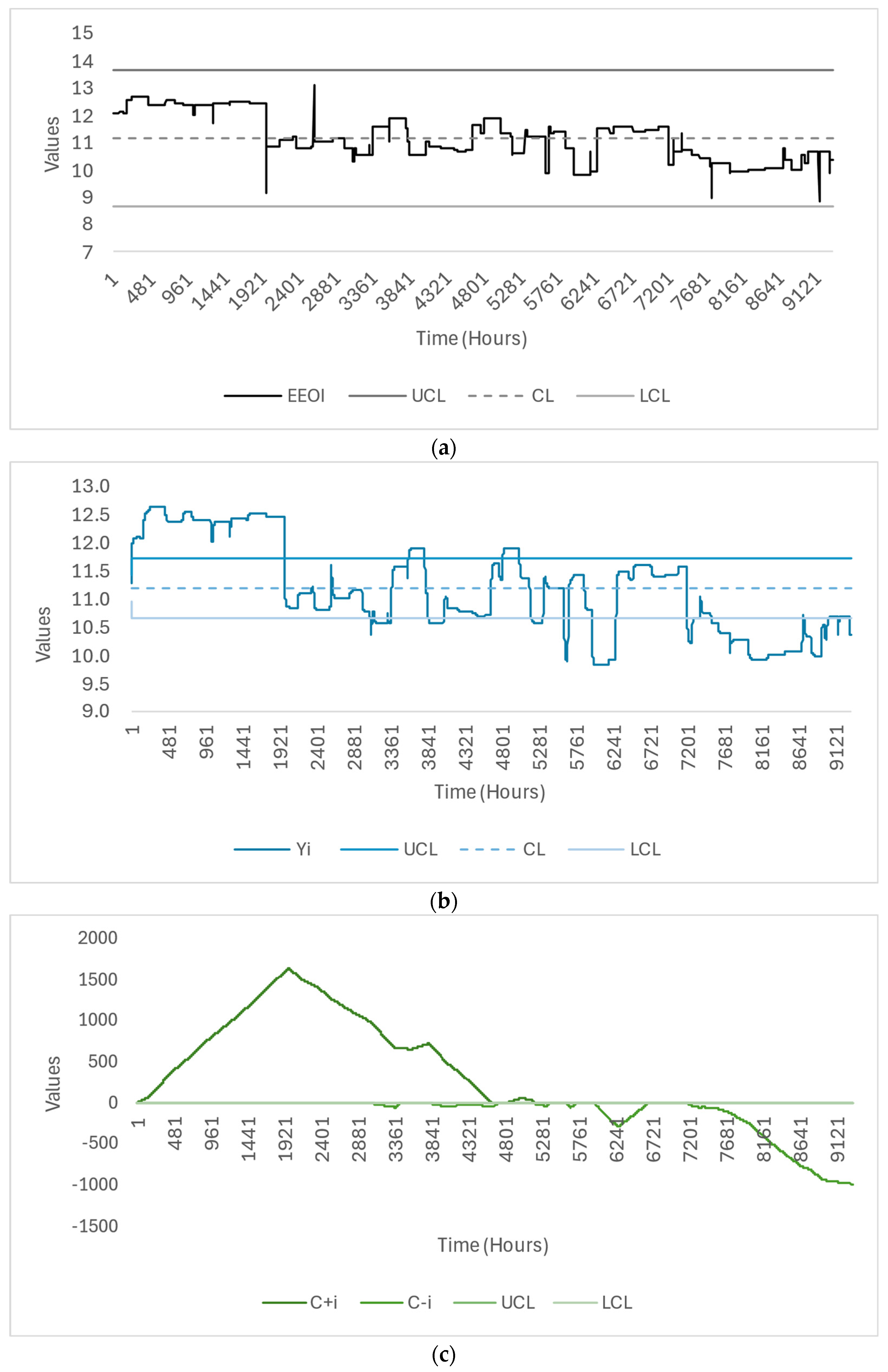
The following graphs (Figure 3) show the representation of the EEOI values with respect to the reference values calculated using representative data extracted from the Kyma 2.0 software database, which records actual voyages and operational conditions of the ship under study. These values correspond to the laden navigation condition, with speeds between 18 and 20 knots.
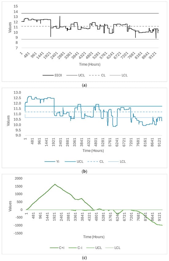
Figure 3.
(a). Shewhart chart for laden condition in range of 18–20 knots; (b). EWMA chart for laden condition in range of 18–20 knots; (c). CUSUM chart for laden condition in range of 18–20 knots.
As mentioned in Table 3, UCL represents the upper control limit, CL is the control line and LCL is the lower control limit. In the EWMA chart, Yi is the variable that is being tracked and created with the current and previous values. C+i and C-i in the CUSUM chart represent the cumulative sums of data that are above and below a certain distance from the control value, respectively. This arrangement applies to all figures representing control charts.
As can be seen in the figure, no anomalies are detected in the Shewhart chart, the CUSUM only reflects anomalous data and the EWMA seems to show a reasonable number of anomalies that, together with the possibility of adjusting the limits, would allow the sensitivity of the method to be regulated, giving value to the continuous improvement procedure.
4.1.2. Analysis of Control Tools in Representative Data of the 18–20 Knot Speed Range, under Ballast Conditions
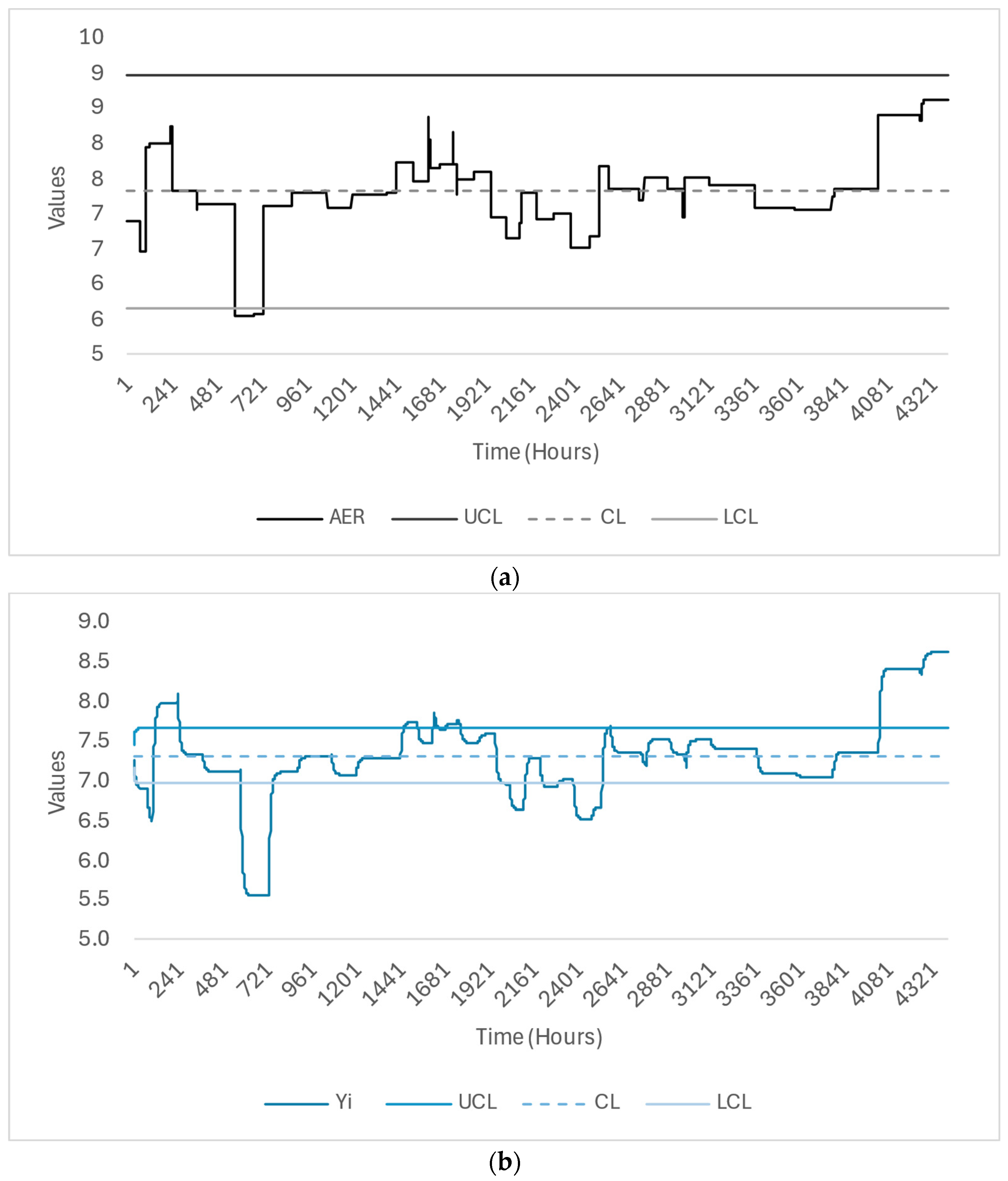
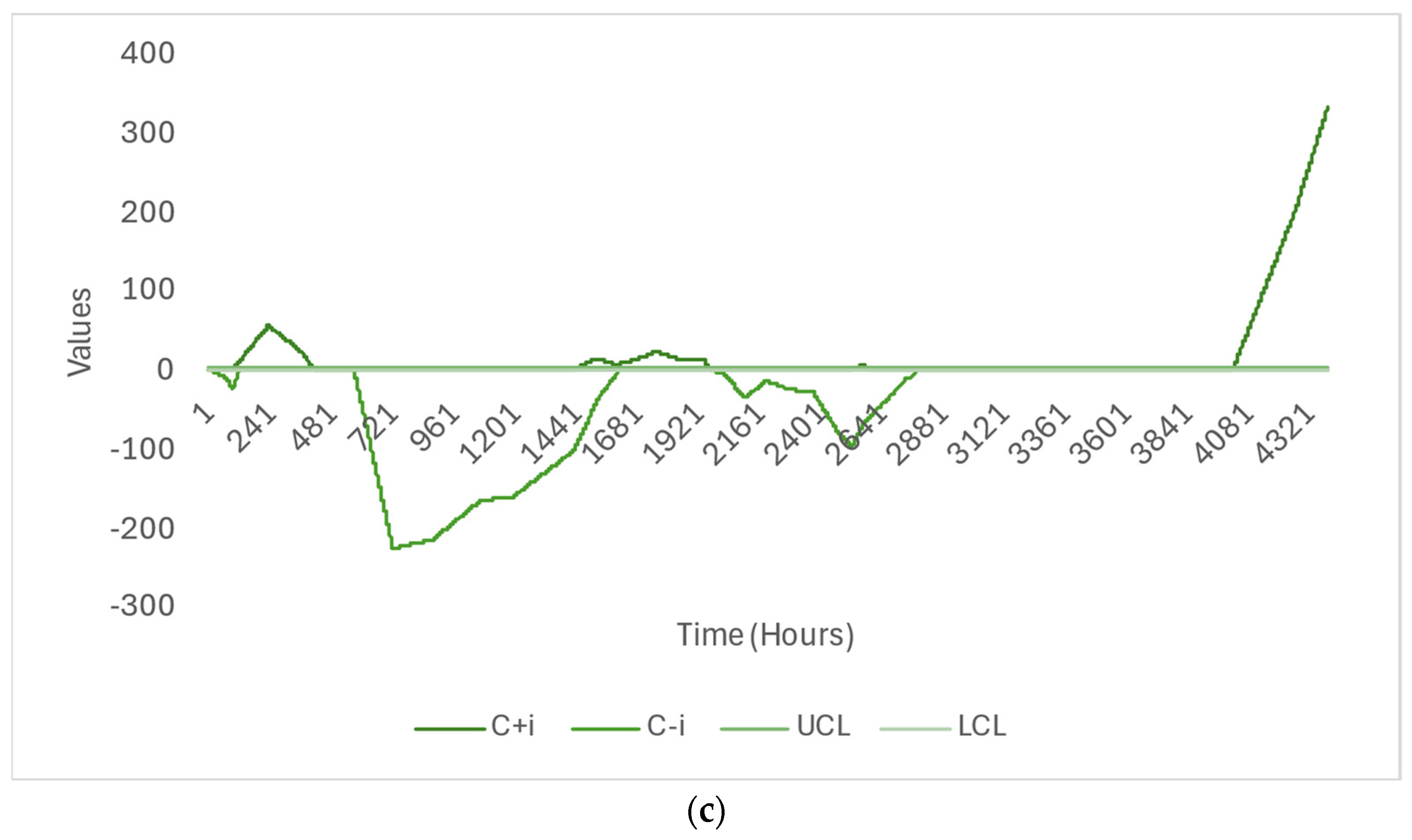
The following graphs (Figure 4) show the representation of the EEOI values with respect to the reference values calculated using representative data extracted from the Kyma software database, which records actual voyages and operational conditions of the ship under study. These values correspond to the ballast navigation condition, with speeds between 18 and 20 knots.
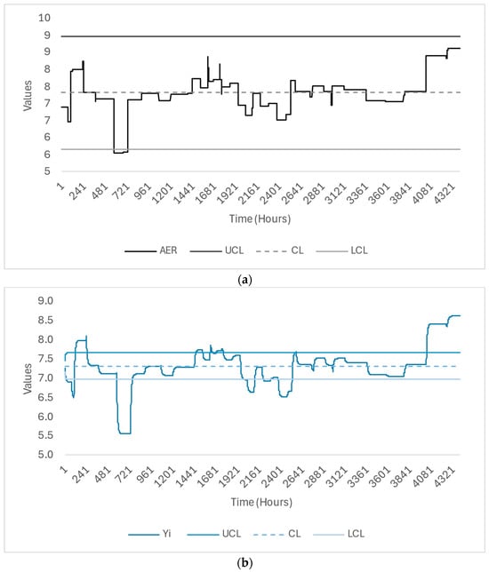

Figure 4.
(a). Shewhart chart of ballast condition in range of 18–20 knots; (b). EWMA chart of ballast condition in range of 18–20 knots; (c). CUSUM chart of ballast condition in range of 18–20 knots.
In this section, what was seen in the case of the load condition has been repeated. With the Shewhart control chart, no anomalies are detected; using the CUSUM control chart, practically all the data are anomalies, but if we use the EWMA control charts, there is a correct detection of anomalies.
In both of these examples, it can be seen that Shewhart charts hardly produce any kind of alerts under any conditions, so they are not very helpful in detecting inefficiencies. Conversely, CUSUM charts are almost permanently in a state of alert because they represent the accumulated sum of data, and it is difficult to bring them back into the control range.
EWMA presents a middle ground between both types of charts, since it detects what would be a reasonable number of anomalies in a representative sample. This is because EWMA evaluates a composite between the present value of the EEOI and a percentage of the previous weighted EEOI values, which makes it evaluate the trend, instead of exclusively evaluating individual values. This characteristic, together with the ability to adapt the control limits to the awareness needs of the system, makes EWMA the ideal control system for the control of the EEOI and its continuous improvement. In the Results and Discussion section, the selected procedure is validated with the vessel’s navigation data and details from the vessel’s logbook.
5. Results and Discussion
The calculation of the Energy Efficiency Operational Index (EEOI) currently faces significant challenges due to the randomness in the selection of data used. Although the IMO has established the standard formula for calculating the EEOI, it has not defined strict criteria on which specific data should be considered to ensure the representativeness of the results. As a consequence, ship operators may employ different approaches to collecting and selecting data, from employing a single specific voyage to averaging multiple voyages. This lack of standardization can lead to significant variations in EEOI results, affecting the accuracy and comparability of energy efficiency assessments between different ships and operators.
It is common in the EEOI calculation methodology to use the average of the last ten voyages. However, this methodology causes representativeness problems by mixing cargo voyages with ballast voyages in the average and by equally weighting short-day voyages with unusual characteristics and more representative long-distance voyages. This mixture can distort the results, since ballast voyages and short voyages can have significantly different fuel consumption and energy efficiency compared to cargo and long-distance voyages. Therefore, the current methodology does not always accurately reflect the operational energy efficiency of a ship under normal operating conditions.
5.1. Discussion of Block I, Selection of Representative Values of the EEOI
This study has detailed the selection of the most representative data on energy efficiency in national and international maritime transport. First, a selection of that data was made based on the conditions of the load or ballast, followed by daily calculations with the actual load data. In this way, we have a reliable indicator of “work transport”. Subsequently, the data were selected by a mode of operation where the ship travels distances transporting cargo. This led to discarding 20.38% of the data, thus maintaining a database that is representative of the transport of merchandise, something that the bibliography that questioned the EEOI as an operational indicator of energy efficiency indicated that the formula lacked. Subsequently, and following the indications of studies by the IMO itself and other researchers, the EEOI and AER values were chosen based on the speed range that is used the longest for the transport of cargo. With all this, we calculated the average EEOI and AER and the standard deviation, thus providing the base values representative of the energy efficiency and emissions of the ship. The results showed that cargo voyages have an average EEOI of around 10.80, while ballast voyages have an average AER of around 6.90. Averaging them gives a value of around 8.37, a value that is not representative of any of the cases but is just a very distorted global average affected by the duration and typology of the voyages.
Numerous publications [9,10,17,23,24,25] have highlighted the importance and influence of speed in the calculation of the EEOI and AER. So, in addition to the difference in energy efficiency between loaded and ballast voyages, a comparison of the EEOI has been made for each sailing speed, both in laden and ballast conditions. The results of this analysis demonstrate that the sailing speed is a key parameter that significantly influences the EEOI. The variability of the EEOI according to sailing speed further highlights the importance of separating the data according to specific operating conditions.
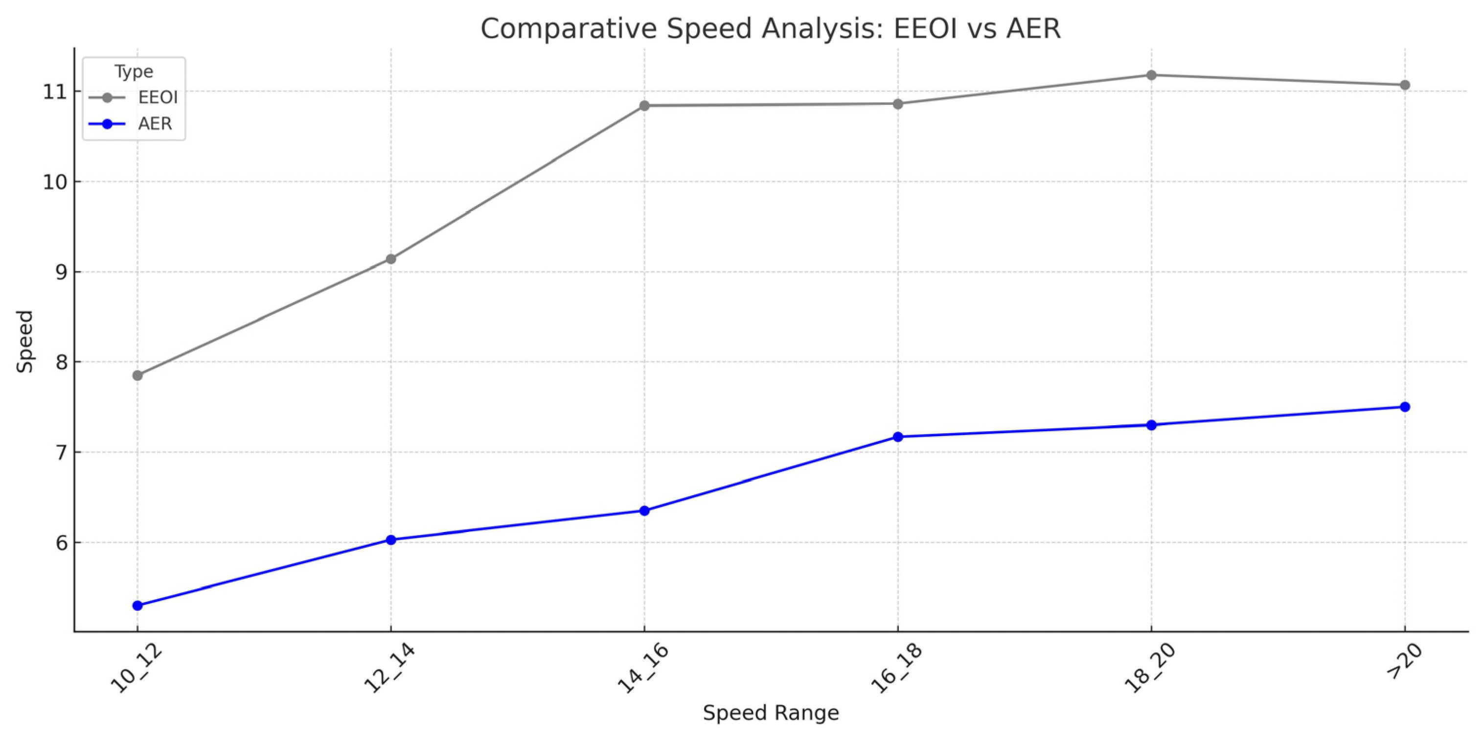
Figure 5 reveals that the EEOI is consistently higher than the AER. This can be attributed to several factors in addition to the calculation formula. Firstly, ballast voyages generally involve higher relative fuel consumption, as the vessel carries ballast water instead of cargo, which increases weight and fuel consumption without generating cargo transportation revenue. Furthermore, in ballast conditions, the weight distribution and resistance of the vessel may not be optimal, leading to higher drag and higher fuel consumption to maintain the same speed [24].
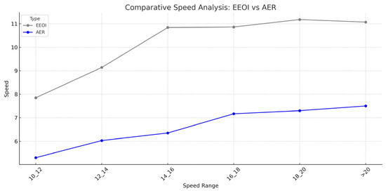
Figure 5.
Comparative analysis of the EEOI and AER mean at the speed ranges.
Similarly, when observing the figure, it can be noted that the EEOI varies considerably with speed, especially between the 14–16 and 10–12 ranges, showing that, at higher speeds, fuel consumption tends to increase, which negatively affects energy efficiency and raises CO2 emissions. This variability demonstrates that an accurate assessment of energy efficiency must consider not only the vessel’s loading condition but also its operating speed. Ignoring these factors and averaging the data indiscriminately can lead to an inaccurate representation of the vessel’s energy performance. However, the EEOI does not increase with speed in all its ranges, since a decrease in the EEOI is observed in the last speed range (more than 20 knots) with respect to the 18–20 range. This is because the speed is above the nominal speed provided by the ship’s propulsion, favoured by weather conditions that push the ship and therefore improve its EEOI. These favourable weather factors increase the speed for the same fuel consumption, contributing to more efficient EEOI values at higher speeds. This does not occur in AER analysis and because, from 14 to 16, the lines flatten out. These results showcase that it is essential to separate the analysis according to the speed ranges.
In addition to observations regarding the variability of the EEOI with speed and loading conditions, the analysis suggests practical strategies to improve the energy efficiency of ships. The data obtained confirms that the EEOI is better at low speeds, and the idea that it would be remarkably interesting to adopt the practice of “slow steaming”, that is, sailing at the lowest possible speed that allows reaching port on the planned date. This practice not only improves energy efficiency, but also avoids the inefficiency of sailing at a higher speed and arriving earlier than necessary. Sailing at a speed optimized for the arrival time reduces fuel consumption and CO2 emissions, contributing to a more sustainable and economical operation.
On the other hand, although it is difficult to avoid ballast voyages in the LNG vessel under study due to commercial transport routes, the data indicates the suitability, in terms of energy efficiency, of reducing ballast voyages and sailing in a loaded condition for the greatest possible percentage of the time. Although LNG vessels must make ballast voyages, optimizing operations to minimize these voyages is crucial. In other types of vessels with comparable results, it would be highly desirable to optimize the load and reduce ballast voyages, since energy efficiency is significantly affected when sailing without cargo.
These approaches not only improve energy efficiency, but also have a positive impact on reducing operating costs and on increasing environmental sustainability.
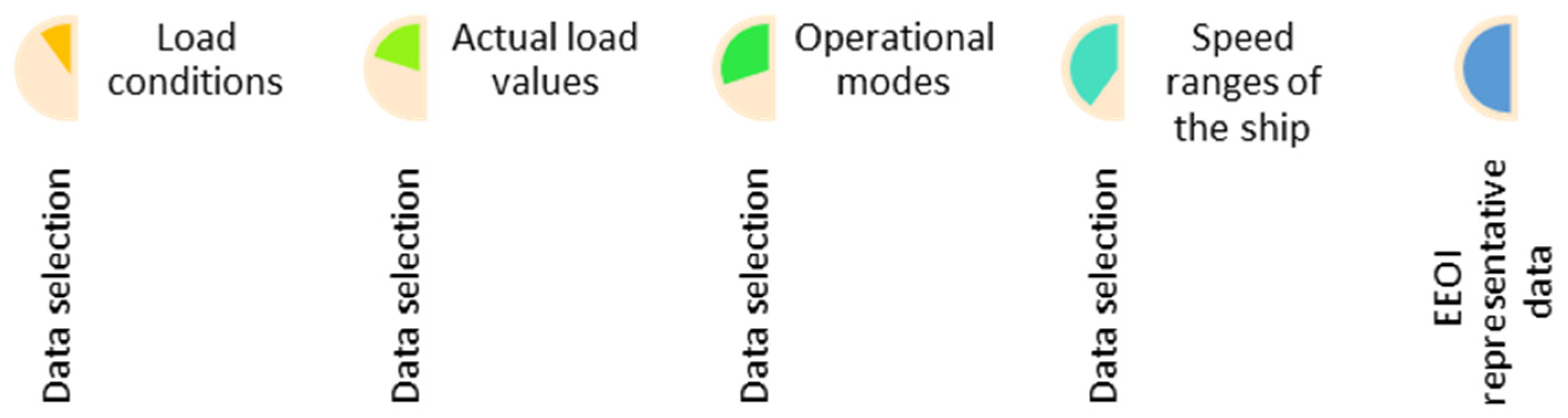
Based on all the above, the results of this study demonstrate the importance of obtaining the EEOI for each load condition (laden and ballast) and ship speed in order to have a representative average EEOI value for each operating condition. In this way, with these values, effective EEOI deviation control systems can be established for each of these conditions, accurately detecting more or less efficient operating periods. All the steps of this procedure can be observed in Figure 6.
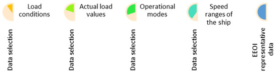
Figure 6.
EEOI data selection procedure to obtain representative values.
5.2. Discussion of Block II, EEOI and AER Control Analysis
One of the great advantages of using the EWMA as a control chart is the flexibility of its parameters. This means that as the continuous improvement procedures progress, the control system can be adjusted through the values of λ and L to make it more or less sensitive and thus better adapt to the process to be monitored.
In the case of the EWMA, to select which parameter values are the most appropriate for working with the data, it is necessary to take into account a factor called Average Run Length (ARL) in control, which considers how long the process can be allowed to be in control without generating false alarms [50]. In our case, the EEOI and AER values are generally stable, but may have sudden changes, so a detection of moderate–large changes (two standard deviations) is selected. In this case, the recommended values are λ of 0.37 and L of 3.047, which presents an ARLmin of 3.5, approximately twenty minutes.
Using these values of λ and L, we will validate the procedure by comparing the out-of-control data with the notes in the navigation log, in such a way that we will check if the out-of-control points given by the procedure occurred in reality and what was the cause that provoked them.
5.2.1. Validation of the EWMA Procedure under Laden Conditions
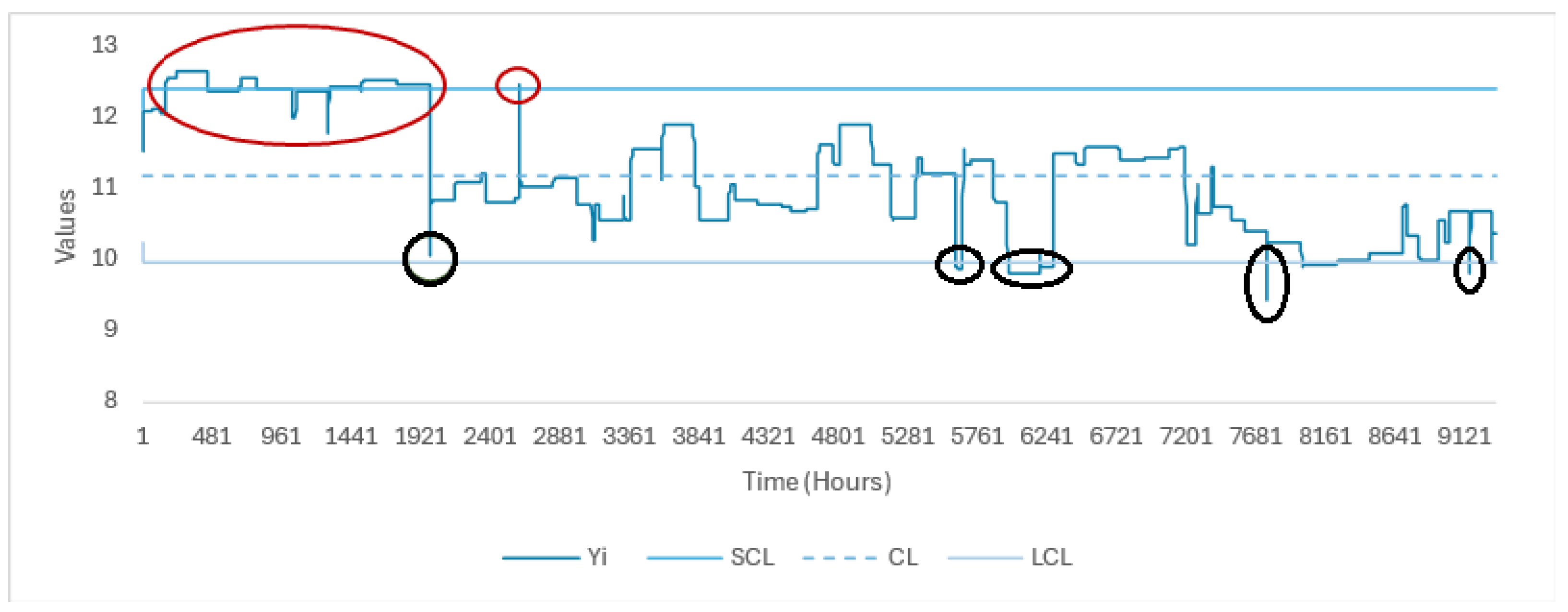
Figure 7 shows the EEOI values with the EWMA control chart, under laden navigation conditions in the speed range of 18–20. The upper out-of-control values are highlighted in red and the lower out-of-control values are highlighted in black.
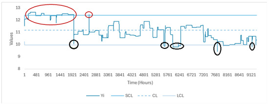
Figure 7.
EWMA of the laden condition at a speed of 18–20 knots.
The only interval that exceeds the upper control limit occurs at the beginning of the series. This was due to one of the engines operating exclusively with MDO, instead of LNG, during a period between the 4th and 11th of September 2023, which was the duration of the maintenance tasks.
The upper control limit was also momentarily exceeded on one occasion on 17 September, as part of the engines were again changed to MDO before passing through the Suez Canal to comply with the canal regulations.
Likewise, during the period under study, the lower control limit was also exceeded on several occasions. The first time the lower limit was exceeded (around the value 1985), it was occasional due to a speed reduction for anchoring and bunkering on 13 September.
Next, there are two short intervals close to the value 5761, where the lower control limit was exceeded again. After analyzing the data in these intervals, it was found that there was a change in the configuration of the propulsion plant, going from four to three engines in operation. This same reason is the cause of the peak that exceeds the LCI around the value 7681 (25 February 2024). This also shows that a high load configuration of three engines is more efficient than a medium load configuration with four engines.
At the end of the interval under study, the LCI is also exceeded since the speed is reduced to anchor while waiting for authorization to enter the port and later after restarting the march and lowering the speed again for docking in the port.
It is notable to mention that, despite there being a considerable number of intervals out of control in this range of speeds, in most cases, the difference between the values and the limits is small, as can be seen in the figure.
5.2.2. Validation of the EWMA Procedure under Ballast Conditions
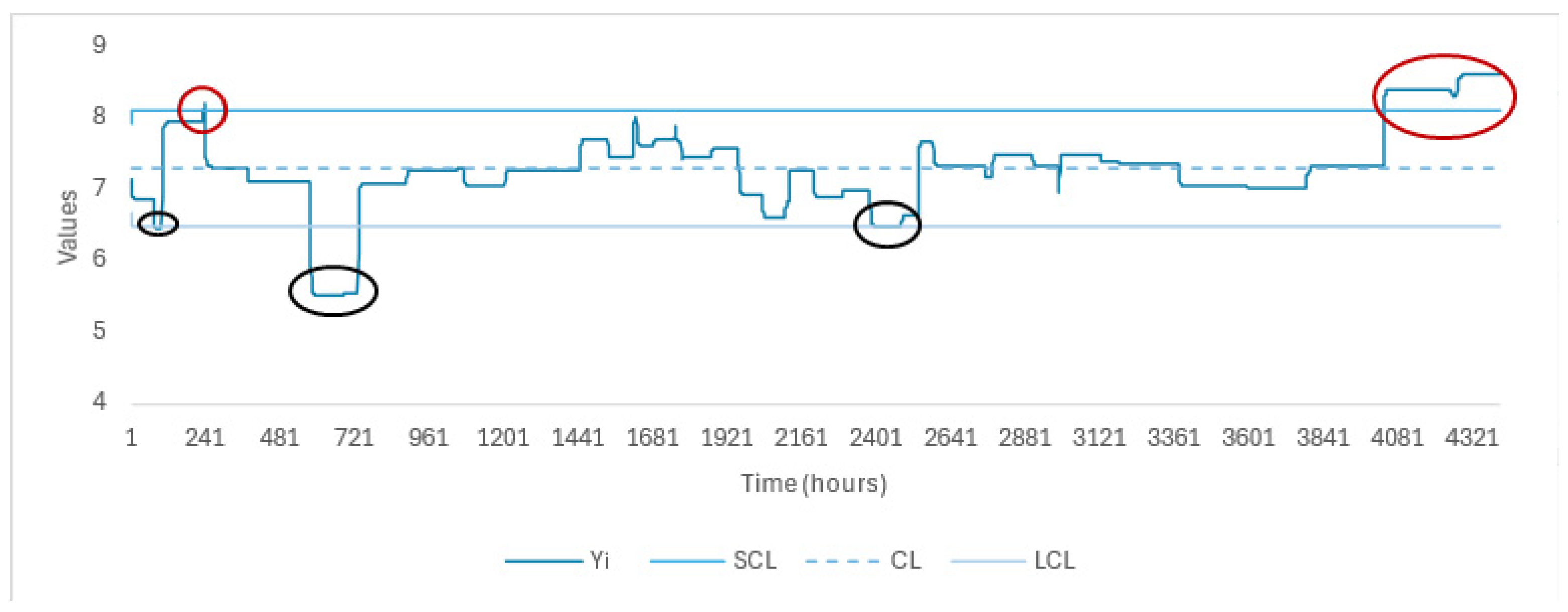
Figure 8 shows the AER values in ballast condition in a range of 18–20 knots, where the higher out-of-control values are highlighted in red and the lower out-of-control values are highlighted in black. In contrast to the laden navigation mode, the number of the out-of-control values is lower.
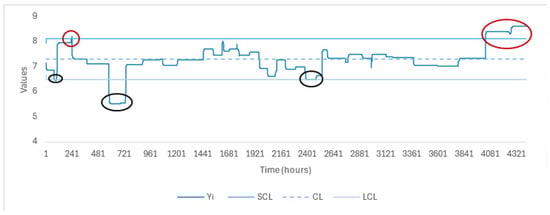
Figure 8.
EWMA of the ballast condition at 18–20 knots.
The first interval that exceeds the lower control limit occurs at the beginning of the series (circled in black). The main reason for the aforementioned excess is that the first recorded trip is of short duration and a configuration of third engines is chosen instead of four, which results in low AER values. Furthermore, at the end of the trip, a brief passage through the speed range of 18–20 is made on the descent ramp.
The second interval (around sample 241, 17 October 2023) occasionally exceeds the UCL. This is due to the fact that some of the engines are changed to MDO, as an anchor stop is made to carry out bunkering.
The third interval represents a considerable drop below the lower control limit (around the value 721, 20 October), in which a configuration of using fewer engines at a higher load is chosen again.
The last notable interval is the final part of the period under study where the use of all engines at a lower load is chosen to deal with the arrival at port. This configuration has a lower performance and begins at point 4034 (First point recorded of 3 March 2024) where it exceeds the upper control limit and does not return to the control interval for the rest of the graph.
The EWMA demonstrates its great effectiveness when determining anomalous EEOI values in the system in addition to helping their classification. A value that exceeds the upper control limit shows an inefficiency that must be corrected and studied so that it can be avoided as much as possible. Likewise, a value that falls below the lower control limit denotes that the process is abnormally efficient, which should also be studied to improve the overall performance of the ship.
6. Conclusions and Future Work
This research introduces a new methodology for calculating the Operational Energy Efficiency Index (EEOI), respecting the formula established by the International Maritime Organization (IMO), that is completely transferable to any type of vessel, which allows the real-time control of the EEOI of the vessel in any navigation situation, load condition, and variation in load and navigation speed.
Having a procedure to obtain the reference values customized for each vessel and transport service is also one of the key results of this study, which for the first time provides a universal procedure that allows quickly having a baseline of emissions for their control and, above all, their improvement. This procedure is based on the selection of the most representative navigational data of the ship’s activity according to its most influential parameters, and this disruptive approach to data preparation is the key to obtaining highly effective EEOI control charts.
Therefore, this makes the SEEMP of the vessels that follow this procedure able to implement continuous improvement measures much more effectively and with guarantees of compliance with the objectives and regulations. On the other hand, the great adaptation of EWMA graphics for the automatic control of EEOI data in real time and the continuous improvement of the emissions and energy efficiency of the ship has also been demonstrated in detail. The “Data Selection—Control by EWMA” set is a highly effective procedure in terms of the control of emissions and energy efficiency of ships. The set of the two measures will make maritime transport resilient and committed to the emissions objectives to stop and reverse climate change.
In future work, we will analyze this procedure for other ship types and further explore the influence and inclusion of meteorological parameters in the EEOI calculation.
Author Contributions
Conceptualization, S.Z. and F.F.D.; methodology, J.B.M.; software, F.F.D.; validation, J.B.M., S.Z. and F.F.D.; investigation, J.B.M., S.Z. and F.F.D.; resources, F.F.D.; data curation, F.F.D.; writing—original draft preparation, J.B.M., S.Z. and F.F.D.; writing—review and editing, J.B.M.; supervision, S.Z. and V.D.-C.; funding acquisition, V.D.-C. All authors have read and agreed to the published version of the manuscript.
Funding
The authors are thankful for financial support from the grant PID2021-122532OB-I00 funded by MCIN/AEI/10.13039/501100011033 and by ERDF A way of making Europe, the project PDC2021-121076-I00 funded by MCIN/AEI/10.13039/501100011033 and by the European Union Next GenerationEU/PRTR and the project ED431C 2022/39 funded by Xunta de Galicia. This publication is part of the grant RYC2021-033040-I, funded by MCIN/AEI/10.13039/501100011033 and from the European Union «NextGenerationEU»/PRTR.
Institutional Review Board Statement
Not applicable.
Informed Consent Statement
Not applicable.
Data Availability Statement
We have uploaded an Excel file that contains the data employed to construct the control charts displayed in this paper.
Conflicts of Interest
The authors declare no conflict of interest.
References
- Issa, M.; Ilinca, A.; Martini, F. Ship energy efficiency and maritime sector initiatives to reduce carbon emissions. Energies 2022, 15, 7910. [Google Scholar] [CrossRef]
- Sogut, M.Z.; Ozkaynak, S. Energy Efficiency and Management Onboard Ships, in Decarbonization of Maritime Transport; Springer Nature: Singapore, 2023; pp. 179–189. [Google Scholar] [CrossRef]
- UN Trade and Developmente, Review of Maritime Transport 2023: Towards a Green and Just Transition, UNCTAD. Available online: https://unctad.org/publication/review-maritime-transport-2023 (accessed on 15 July 2024).
- Dewan, M.H.; Godina, R. Seafarers involvement in implementing energy efficiency operational measures in maritime industry. Procedia Comput. Sci. 2023, 217, 1699–1709. [Google Scholar] [CrossRef]
- Internationa Maritime Organization. IMO-Energy Efficiency Measures, 17 August 2009. Available online: https://gmn.imo.org/wp-content/uploads/2017/05/Circ-684-EEOI-Guidelines.pdf (accessed on 16 June 2024).
- Ivanova, G.; Donev, I.; Kostova, I. Study of the Influence of the Physical Environment on the Design and Operational Indices of Energy Efficiency EEDI and EEOI. In Proceedings of the 2020 12th Electrical Engineering Faculty Conference (BulEF), Varna, Bulgaria, 9–12 September 2020. [Google Scholar] [CrossRef]
- Tran, T.A. A research on the energy efficiency operational indicator EEOI calculation tool on M/V NSU JUSTICE of VINIC transportation company, Vietnam. J. Ocean. Eng. Sci. 2017, 2, 55–60. [Google Scholar] [CrossRef]
- MEPC.1/Circ.684; Guidelines For Voluntary Use of the Ship Energy Efficiency Operational Indicator (EEOI). The Marine Environment Protection Committee (MEPC): London, UK, 2009; p. 12.
- Poulsen, R.T.; Viktorelius, M.; Varvne, H.; Rasmussen, H.B.; von Knorring, H. Energy efficiency in ship operations-Exploring voyage decisions and decision-makers. Transp. Res. Part D Transp. Environ. 2022, 102, 103120. [Google Scholar] [CrossRef]
- Yehia, W.; Kamar, L.; Mosaad, H.; Moustafa, M. Improving Container Ship’s Energy Efficiency Operational Indicator (EEOI) by Speed Management. Port-Said Eng. Res. J. 2021, 25, 59–65. [Google Scholar] [CrossRef]
- Perez, J.R.; Reusser, C.A. Optimization of the emissions profile of a marine propulsion system using a shaft generator with optimum tracking-based control scheme. J. Mar. Sci. Eng. 2020, 8, 221. [Google Scholar] [CrossRef]
- Tran, T.A. Simulation and analysis on the ship energy efficiency operational indicator for bulk carriers by Monte Carlo simulation method. Int. J. Model. Simul. Sci. Comput. 2020, 11, 2050036. [Google Scholar] [CrossRef]
- Kanberoğlu, B.; Kökkülünk, G. Assessment of CO2 emissions for a bulk carrier fleet. J. Clean. Prod. 2021, 283, 124590. [Google Scholar] [CrossRef]
- Elkafas, A.G.; Shouman, M.R. Assessment of energy efficiency and ship emissions from speed reduction measures on a medium sized container ship. Int. J. Marit. Eng. 2021, 163. [Google Scholar] [CrossRef]
- Chen, X.; Lv, S.; Shang, W.; Wu, H.; Xian, J.; Song, C. Ship energy consumption analysis and carbon emission exploitation via spatial-temporal maritime data. Appl. Energy 2024, 360, 122886. [Google Scholar] [CrossRef]
- Hanghou, Y.; Kang, K.; Liang, X. Vessel speed optimization for minimum EEOI in ice zone considering uncertainty. Ocean. Eng. 2019, 188, 106240. [Google Scholar] [CrossRef]
- Liu, B.; Gao, D.; Yang, P.; Hu, Y. An energy efficiency optimization strategy of hybrid electric ship based on working condition prediction. J. Mar. Sci. Eng. 2022, 10, 1746. [Google Scholar] [CrossRef]
- Wang, K.; Yuan, Y.; Yan, X.; Tang, D.; Ma, D. Design of ship energy efficiency monitoring and control system considering environmental factors. In Proceedings of the 2015 International Conference on Transportation Information and Safety (ICTIS), Wuhan, China, 25–28 June 2015. [Google Scholar] [CrossRef]
- Chi, H.; Pedrielli, G.; Ng, S.H.; Kister, T.; Bressan, S. A framework for real-time monitoring of energy efficiency of marine vessels. Energy 2018, 145, 246–260. [Google Scholar] [CrossRef]
- Fan, A.; Yan, X.; Bucknall, R.; Yin, Q.; Ji, S.; Liu, Y.; Song, R.; Chen, X. A novel ship energy efficiency model considering random environmental parameters. J. Mar. Eng. Technol. 2020, 19, 215–228. [Google Scholar] [CrossRef]
- Capezza, C.; Coleman, S.; Lepore, A.; Palumbo, B.; Vitiello, L. Ship fuel consumption monitoring and fault detection via partial least squares and control charts of navigation data. Transp. Res. Part D Transp. Environ. 2019, 67, 375–387. [Google Scholar] [CrossRef]
- Fan, A.; Li, Y.; Liu, H.; Yang, L.; Tian, Z.; Li, Y.; Vladimir, N. Development trend and hotspot analysis of ship energy management. J. Clean. Prod. 2023, 389, 135899. [Google Scholar] [CrossRef]
- Poulsen, R.T.; Ponte, S.; Van Leeuwen, J.; Rehmatulla, N. The potential and limits of environmental disclosure regulation: A global value chain perspective applied to tanker shipping. Glob. Environ. Politics 2021, 21, 99–120. [Google Scholar] [CrossRef]
- Polakis, M.; Zachariadis, P.; Kat, J.O.D. The energy efficiency design index (EEDI). In Sustainable Shipping: A Cross-Disciplinary View; Springer: Cham, Switzerland, 2019; pp. 93–135. [Google Scholar] [CrossRef]
- Zhang, S.; Li, Y.; Yuan, H.; Sun, D. An alternative benchmarking tool for operational energy efficiency of ships and its policy implications. J. Clean. Prod. 2019, 240, 118223. [Google Scholar] [CrossRef]
- Masodzadeh, P.G. Ship Energy Management Self-Assessment (SEMSA) an Introduction to New Set of Rules and Standards in Operation Mode. Master’s Dissertation, World Maritime University, Malmö, Sweden, 2018. [Google Scholar]
- Faber, J.; Markowska, A.; Nelissen, D.; Davidson, M.; Eyring, V.; Cionni, I.; Selstad, E.; Kågeson, P.; Lee, D.; Buhaug, Ø. Technical Support for European Action to Reducing Greenhouse Gas Emissions from International Maritime Transport; CE Delft: Delft, The Netherlands, 2009. [Google Scholar]
- Masodzadeh, P.G.; Ölçer, A.I.; Ballini, F.; Christodoulou, A. How to bridge the short-term measures to the Market Based Measure? Proposal of a new hybrid MBM based on a new standard in ship operation. Transp. Policy 2022, 118, 123–142. [Google Scholar] [CrossRef]
- RESOLUTION MEPC. 231(65); Guidelines for Calculation of Reference Lines for Use with the Energy Efficiency Design Index (EEDI). The Marine Environment Protection Committee (MEPC): London, UK, 2013.
- International Maritime Organization. 2021 Guidelines on Survey and Certification of the Attained Energy Efficiency Existing Ship Index (EEXI); International Maritime Organization: London, UK, 2021. [Google Scholar]
- International Maritime Organization. 2021 Guidelines on the Operational Carbon Intensity Rating of Ships (CII Rating Guidelines, G4); International Maritime Organization: London, UK, 2021. [Google Scholar]
- International Maritime Organization. Fourth Greenhouse Gas Study 2020. 2020. Available online: https://www.imo.org/en/OurWork/Environment/Pages/Fourth-IMO-Greenhouse-Gas-Study-2020.aspx (accessed on 29 July 2024).
- Perera, L.P.; Mo, B. Emission control based energy efficiency measures in ship operations. Appl. Ocean. Res. 2016, 60, 29–46. [Google Scholar] [CrossRef]
- Kim, S.-H.; Roh, M.I.; Oh, M.J.; Park, S.W.; Kim, I.I. Estimation of ship operational efficiency from AIS data using big data technology. Int. J. Nav. Archit. Ocean. Eng. 2020, 12, 440–454. [Google Scholar] [CrossRef]
- Zhang, S.; Yuan, H.; Sun, D. Fluctuation in operational energy efficiency of ships and its implications for performance appraisal. Int. J. Nav. Archit. Ocean. Eng. 2021, 13, 367–378. [Google Scholar] [CrossRef]
- Chen, X.; Lv, S.; Wu, B.; Li, C.; Xian, J.; Wu, H. Ship Energy Efficiency Operation Index Variation Analysis Via Empirical Voyage Data. In Proceedings of the 2023 7th International Conference on Transportation Information and Safety (ICTIS), Xi’an, China, 4 August 2023. [Google Scholar] [CrossRef]
- Cepowski, T.; Kacprzak, P. Reducing CO2 Emissions through the Strategic Optimization of a Bulk Carrier Fleet for Loading and Transporting Polymetallic Nodules from the Clarion-Clipperton Zone. Energies 2024, 17, 3383. [Google Scholar] [CrossRef]
- Sardar, A.; Anantharaman, M.; Islam, T.R.; Garaniya, V. Data collection framework for enhanced carbon intensity indicator (CII) in the oil tankers. Can. J. Chem. Eng. 2024. [Google Scholar] [CrossRef]
- Zhu, Y.; Zuo, Y.; Li, T. Modeling of Ship Fuel Consumption Based on Multisource and Heterogeneous Data: Case Study of Passenger Ship. J. Mar. Sci. Eng. 2021, 9, 273. [Google Scholar] [CrossRef]
- Hu, Z.; Zhou, T.; Osman, M.T.; Li, X.; Jin, Y.; Zhen, R. A novel hybrid fuel consumption prediction model for ocean-going container ships based on sensor data. J. Mar. Sci. Eng. 2021, 9, 449. [Google Scholar] [CrossRef]
- Perera, L.P.; Mo, B.; Kristjánsson, L.A.; Jønvik, P.C.; Svardal, J. Evaluations on ship performance under varying operational conditions. In Proceedings of the International Conference on Offshore Mechanics and Arctic Engineering, St. John’s, NL, Canada, 31 May–5 June 2015. [Google Scholar] [CrossRef]
- Yan, R.; Yang, D.; Wang, T.; Mo, H.; Wang, S. Improving ship energy efficiency: Models, methods, and applications. Appl. Energy 2024, 368, 123132. [Google Scholar] [CrossRef]
- Acomi, N.; Acomi, O.C. Improving the voyage energy efficiency by using EEOI. Procedia-Soc. Behav. Sci. 2014, 138, 531–536. [Google Scholar] [CrossRef]
- Sun, C.; Wang, H.; Liu, C.; Zhao, Y. Real Time Energy Efficiency Operational Indicator (EEOI): Simulation Research from the Perspective of Life Cycle Assessment. J. Phys. Conf. Ser. 2020, 1626, 012060. [Google Scholar] [CrossRef]
- Gao, C.-F.; Hu, Z.-H. Speed optimization for container ship fleet deployment considering fuel consumption. Sustainability 2021, 13, 5242. [Google Scholar] [CrossRef]
- Pelić, V.; Bukovac, O.; Radonja, R.; Degiuli, N. The impact of slow steaming on fuel consumption and CO2 emissions of a container ship. J. Mar. Sci. Eng. 2023, 11, 675. [Google Scholar] [CrossRef]
- Koutras, M.V.; Bersimis, S.; Maravelakis, P. Statistical process control using Shewhart control charts with supplementary runs rules. Methodol. Comput. Appl. Probab. 2007, 9, 207–224. [Google Scholar] [CrossRef]
- Abbas, N.; Riaz, M.; Does, R.J. Mixed Exponentially Weighted Moving Average–Cumulative Sum Charts for Process Monitoring. Qual. Reliab. Eng. Int. 2013, 29, 345–356. [Google Scholar] [CrossRef]
- Montes, J.B.; Fernández, S.Z.; Casas, V.D. Internet of the things in Energy-Sensitive processes: Application in a refrigerated warehouse. IEEE Access 2024, 12, 76257–76276. [Google Scholar] [CrossRef]
- Lucas, J.M.; Saccucci, M.S. Exponentially weighted moving average control schemes: Properties and enhancements. Technometrics 1990, 32, 1–12. [Google Scholar] [CrossRef]
- Montgomery, C. Introduction to Statistical Quality Control; John Wiley & Sons: Hoboken, NJ, USA, 2019. [Google Scholar]
- Ryan, T.P. Statistical Methods for Quality Improvement; John Wiley & Sons: Hoboken, NJ, USA, 2011. [Google Scholar]
- Page, S. Continuous inspection schemes. Biometrika 1954, 41, 100–115. [Google Scholar] [CrossRef]
Disclaimer/Publisher’s Note: The statements, opinions and data contained in all publications are solely those of the individual author(s) and contributor(s) and not of MDPI and/or the editor(s). MDPI and/or the editor(s) disclaim responsibility for any injury to people or property resulting from any ideas, methods, instructions or products referred to in the content. |
© 2024 by the authors. Licensee MDPI, Basel, Switzerland. This article is an open access article distributed under the terms and conditions of the Creative Commons Attribution (CC BY) license (https://creativecommons.org/licenses/by/4.0/).