Abstract
In the era of marine big data, making full use of multi-source satellite observations to accurately retrieve and predict the temperature structure of the ocean subsurface layer is very significant in advancing the understanding of oceanic processes and their dynamics. Considering the time dependence and spatial correlation of marine characteristics, this study employed the convolutional long short-term memory (ConvLSTM) method to retrieve the subsurface temperature in the Western Pacific Ocean from several types of satellite observations. Furthermore, considering the temperature’s vertical distribution, the retrieved results for the upper layer were iteratively used in the calculation for the deeper layer as input data to improve the algorithm. The results show that the retrieved results for the 100 to 500 m depth temperature using the 50 m layer in the calculation resulted in higher accuracy than those retrieved from the standard ConvLSTM method. The largest improvement was in the calculation for the 100 m layer, where the thermocline was located. The results indicate that our improved ConvLSTM method can increase the accuracy of subsurface temperature retrieval without additional input data.
1. Introduction
It is well established that marine data are essential for oceanology and climate change research. However, observing the ocean is difficult and expensive, so it remains rare. Although implementing the Argo program has dramatically enhanced global ocean observations since 2004, the program still needs improvement regarding the observation density, distribution, and time span due to the limitations of the observation means and cost [1,2]. On the other hand, with the development of satellite remote sensing technology, the remotely sensed sea surface temperature and sea surface height information are increasing, providing many images of the ocean’s surface with comprehensive coverage, a high spatial resolution, and strong temporal continuity [3,4].
These abundant satellite data only reflect the ocean’s surface; researchers need more data to determine the structure and variation under the surface. The three-dimensional dynamical processes within the ocean are very complex, and many crucial physical ocean phenomena and dynamical processes exist within a certain depth range below the surface [5,6,7]. The subsurface structure of the ocean, especially the temperature structure, needs to be accurately studied to understand the ocean’s circulation, the thermocline structure, and climate change. Researchers are trying to utilize satellite data to compensate for the insufficiency of the data obtained inside the ocean.
Artificial intelligence (AI) technology, driven by data, extracts valuable information from data through multi-layer learning and objectively mines the intrinsic relationships between data, which not only improves the efficiency and precision of data processing, breaking the bottlenecks of traditional technology, but also brings a new opportunity for the intelligent analysis and excavation of marine big data. In recent years, machine learning and deep learning have also been applied to retrieve the ocean’s subsurface structure. Ali used an artificial neural network (ANN) to retrieve the vertical temperature structure through SST, SSH, and other sea surface flux parameters [8]. Wu used a self-organizing neural network (SOM) to build a network through Argo grid data to retrieve the subsurface temperature anomalies using remotely sensed data [9]. Su used a support vector machine (SVM) to study the Indian Ocean 1000 m above the subsurface temperature anomaly [10]. Su proposed a geographically weighted regression (GWR) method to retrieve the global subsurface temperature anomaly through multi-source satellite data and took into account the significant spatial non-stationarity between the ocean surface parameters and the subsurface parameters in the model [11]. Cheng proposed incorporating a new sea surface parameter, SSV, to retrieve the subsurface temperature in the Northern Pacific [12]. Su proposed improving the generalization ability of the prediction model by incorporating time series feature learning using a long short-term memory neural network (LSTM) [13]. Although the LSTM [14] algorithm, as a specific deep learning algorithm, can effectively consider the time dependence of marine data, it cannot be efficiently trained on the spatial scale to deal with the spatial nonlinearities of marine data simultaneously [15,16,17]. Considering the spatial correlation of ocean data, convolutional-neural-network-related deep learning algorithms have also been widely applied to subsurface temperature retrieval in recent years. Han proposed using a convolutional neural network (CNN) to incorporate spatial sequence feature learning to build a monthly CNN model to reconstruct the subsurface temperature. However, the monthly CNN model did not subtract the corresponding feature climate averages, and the single-point model lacked a certain degree of universality [18]. Meng proposed utilizing a convolutional neural network to retrieve the subsurface temperature in the Pacific region and improve the horizontal resolution from 1° to 1/4° [19]. Shi et al. proposed the retrieval of the subsurface temperature with a convolutional long short-term memory (ConvLSTM) network algorithm, which takes into account the spatial and temporal characteristics of ocean data together and combines the spatial information in the time series to improve the accuracy of the model prediction [20]. Song et al. then applied the method to atmospheric wind field forecasting and obtained accurate large-scale forecasts [21]. The method can also combine several surface factors to retrieve the subsurface parameters of other ocean variables (e.g., currents and eddies).
Using deep learning methods, the relationships between ocean elements can be addressed quickly, and the mapping relationship between the surface layer and subsurface layer can be constructed with a low computational cost and high efficiency.
The tropical Western Pacific is well known as the “warm pool” of the global ocean, featuring the highest global sea surface temperature and acting as the most important global heat source. The water temperature variation in this area plays an important role in regulating global warming and the climate system. The occurrence of EI Niño in the Central and Eastern Pacific Ocean significantly impacts global climate change [22,23], and many scholars have found that the Western Pacific’s water temperature is closely related to El Niño [24,25,26,27]. Moreover, further studies have emphasized that the water temperature variation in the tropical Western Pacific plays a critical role in the EI Niño–Southern Oscillation (ENSO) cycling mechanism [28,29]. Additionally, the variation in the water temperature in the Western Pacific is closely related to the frequent occurrence of droughts and floods in East Asia in recent decades [30,31]. Therefore, retrieving and predicting the structure and variation in the water temperature in the Western Pacific could advance our understanding of the mechanism of the ENSO cycle and climate change and enhance our ability to defend against natural disasters.
In this study, we adopted the ConvLSTM network to retrieve the three-dimensional temperature structure in the Western Pacific area and improved the calculation by taking into account the vertical distribution features of the temperature. Firstly, we retrieved the 50 m layer temperature based on multi-source sea surface parameters and then took the result as an additional input to retrieve the temperatures of deeper layers. In this way, we improved the accuracy of the retrieval of the subsurface layers, especially the 100 m layer, without adding new input data.
The rest of the paper is organized as follows. Section 2 describes the data and methods used in this study. Section 3 presents the error metrics and retrieval results used to evaluate the performance of the prediction model. Section 4 and Section 5 provide the discussion and the conclusions of the study, respectively.
2. Materials and Methods
2.1. Materials
The research area is shown in Figure 1. The range of the area is 135.125° E–154.875° E, 5.125° N–19.875° N. In this study, we calculated the subsurface temperature from multi-source satellite observations, including the sea surface height (SSH), sea surface temperature (SST), and eastward and northward components of the sea surface winds (USSW and VSSW). Three-dimensional water temperature reanalysis data were used to train the model and to validate the model results. The SSH data were acquired from the Archiving, Validation, and Interpretation of Satellite Oceanographic (AVISO) (https://www.aviso.altimetry.fr/en/data/products, accessed on 1 March 2023), which spans the period from January 1993 to the present; the SST data were from OISST version 2.1 (https://www.ncei.noaa.gov/data/sea-surface-temperature-optimum-interpolation/v2.1/, accessed on 1 March 2023), which spans from September 1981 to the present; the SSW data were from CCMP version 3.0 (https://data.remss.com/ccmp/v03.0/, accessed on 1 March 2023), which spans from January 1993 to December 2019; and the reanalysis water temperature data were from the CMEMS dataset, acquired from Copernicus Marine Service (https://data.marine.copernicus.eu/product/GLOBAL_MULTIYEAR_PHY_001_030/, accessed on 1 October 2023), which spans January 1993 through December 2022. To standardize the resolution of the data in model training, the spatial resolution of all parameters was 0.25° × 0.25°, and the temporal resolution was monthly averaging with a time span of January 1993 to December 2018. The CMEMS dataset includes 75 standard depth layers, but only the first 10 layers were used in this study (for 20, 50, 100, 150, 200, 300, 500, 1000, 1500, and 2000 m). The temporal resolution of all parameters was monthly.
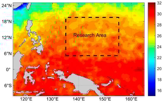
Figure 1.
Map of the research area, denoted by a dashed rectangle (135.125° E–154.875° E, 5.125° N–19.875° N).
The mean values from 2005 to 2018 were first subtracted from all remotely sensed variables (SST, SSH, USSW, and VSSW) to obtain their anomalies and reduce the calculation cost. The subsurface temperature, as the corresponding label for model training and testing, was the main element in assessing the quality of the model.
2.2. Method
The LSTM [14] is a particular type of recurrent neural network that can effectively reflect time continuity and address time series forecasting problems. The CNN is commonly used in image and video processing to extract the complex spatial features of data. The ConvLSTM algorithm, proposed by Shi et al. for spatial–temporal prediction, takes advantage of both [20]. ConvLSTM is a type of deep feed-forward neural network with advantages in extracting local features and weight sharing. It is capable of predicting the temporal variation in the spatial structure of data by switching the fully connected operation of the LSTM algorithm to a convolutional operation. It can also progressively extract more and more complex features and then greatly reduce the number of parameters through the superposition of multiple network layers. Combining the convolutional structure with the recurrent structure allows more complicated spatial–temporal features to be learned in the time series of three-dimensional data. The problem of spatial discontinuity in the prediction results of traditional models, which is usually caused by the inability to recognize the influence of data’s spatial variation, can then be avoided in this way. The hyperparameters in the ConvLSTM model can be adjusted as the research objectives change, and the model’s training efficiency and prediction accuracy can be effectively improved through configuring the model by adjusting the hyperparameters. Considering the strong temporal continuity and spatial correlation of marine data, ConvLSTM, with all its aforementioned advantages, is quite suitable and is now widely used in dealing with oceanographic issues [32,33].
In this study, we used ConvLSTM and determined the optimal configuration of the hyperparameters using the grid searching method. We experimentally considered several combinations of ConvLSTM networks with different layers and finally selected a model with two layers of Convlstm2D and one layer of Conv3D. The complexity of the neural network was reduced by adding regularized Dropout layers between the ConvLSTM layers to avoid the overfitting phenomenon, so that the weights were dispersed and the model did not rely too much on one or some features. The appropriate batch_size was determined based on the results of sensitivity experiments to optimize the model training speed and convergence speed. The nonlinear Relu function was chosen as the activation function for the 2D layer of ConvLSTM, which can not only help to improve the nonlinear fitting ability of the model and reduce the complexity of the model with its sparsity, but also has the advantages of good computational efficiency and interpretability, fast convergence, and reducing incidents of gradient disappearance. The specific settings of the ConvLSTM parameters finalized for this study are shown in Table 1.

Table 1.
ConvLSTM model parameters.
2.3. Experimental Setup
The model architecture for the retrieval of the ocean subsurface temperature field using ConvLSTM is illustrated in Figure 2. The horizontal distributions of the sea surface parameters at moments t − 2, t − 1, and t were input into the ConvLSTM model, and the subsurface temperature at the target depth at moment t was output. Data from January 1993 to December 2018 (312 months in total) were used in the experiments, where 80% of the samples were randomly selected as the training set (20% of which were used as the validation set), and the remaining 20% were used as the test set.
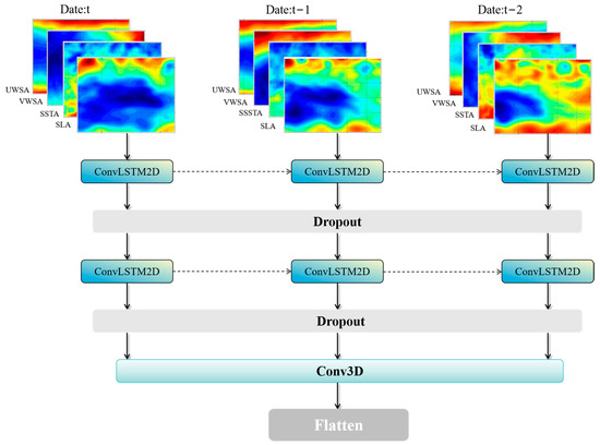
Figure 2.
Model architecture diagram of ConvLSTM.
Considering the physical regulations inside the ocean, and in order to improve the accuracy of the subsurface layer retrieval, the subsurface temperature prediction results of the upper layer were iterated into the retrieval of the lower layer as additional input data. Specifically, the model output of the 50 m layer was added to this study’s calculation of the 100 to 500 m layer. Two groups of comparative experiments for the 100–500 m layers were carried out: in one group, the results were directly retrieved from remote sensing data with the standard ConvLSTM method, and in the other group, the 50 m layer’s results were input into the models for deeper layers. Figure 3 shows the flowchart of our technical route, which included three steps: training dataset construction, model training, and model prediction. For the iterative modeling process, the model prediction of the 50 m layer was added to the input data for the deeper layers’ (100–500 m) model training.
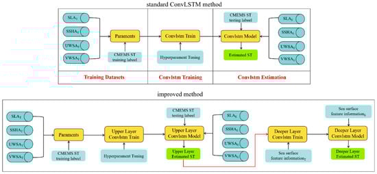
Figure 3.
The workflow charts of the standard ConvLSTM method (upper) and improved method (lower).
In data preprocessing, the input to ConvLSTM is a set of five-dimensional tensors that need to be reconstructed in the shape of (N_samples, N_steps, N_rows, N_columns, N_channels), where N_samples is the total number of input samples, N_steps denotes the number of time steps included in one sample, N_rows and N_columns reflect the input data’s spatial dimensions, and N_channels is the number of channels of the input data. In this study, since the spatial dimension of the input image is 60 × 80, N_rows is 60 and N_columns is 80. N_steps is 3 (t − 2, t − 1, t), N_channels is 4 in the standard ConvLSTM method, and N_channels is 5 in the improved model. Considering the existence of different orders of magnitude of the parameters in the input data, normalization is performed before inputting the model.
The RMSE and R2 are used as indicators to quantitatively evaluate the results.
In the equations, is the true value at time i, i.e., the temperature from the CMEMS data at time i for a certain location and layer; is the corresponding prediction, i.e., the retrieved temperature at time I for the same point; is the number of samples; and is the average of the true values.
3. Results
3.1. Results Retrieved Directly from Sea Surface Data with Standard ConvLSTM Model
We used the standard ConvLSTM method to build the model and retrieved the 0–2000 m (10 layers) subsurface temperatures by inputting sea surface anomaly data. Each layer of the subsurface temperature was calculated one by one, and the models were independent of each other. Along with their corresponding CMEMS data, 80% of the dataset was selected randomly as the input data for model training. After the models were built, the remaining 20% of the dataset was used for the subsurface temperature as test data. The results were compared with the corresponding temperature data from the CMEMS dataset to verify the accuracy of the model prediction. The comparison method was mainly used to calculate the RMSE and R2 between them.
Figure 4 shows the vertical profiles of the errors (RMSE, R2) from the standard ConvLSTM method. The RMSE rises gradually in the 0–150 m range and reaches a maximum of 150 m. Below this, with an increase in depth, the RMSE gradually decreases. Finally, the variation in the RMSE tends to flatten out as the depth increases below a 1000 m depth. The average RMSEs at 100, 150, and 200 m were 0.59, 0.76, and 0.65°, respectively. It can be seen that the errors around 100–200 m are extremely large, showing a peak in the curve. The R2 shows a tendency to decrease, then increase, and then decrease again, with values of 0.75, 0.90, 0.96, and 0.98 at depths of 100, 150, 200, and 300 m, respectively. The R2 value decreases steadily below the depth of the 300 m layer, which reflects the decrease in the model’s prediction ability. The reasons for these phenomena will be discussed in Section 4.2. Table 2 shows the RMSE and R2 of the results from the standard ConvLSTM method for the 100–500 m layer test sets. In the 100 m layer, the root-mean-square error (RMSE) increases with seasonal changes, with a minimum of 0.51 in the spring and a maximum of 0.66 in the winter; in the 150 m layer, the RMSE increases, then decreases, and then increases with seasonal progression, with a maximum in the summer and a minimum in the fall.
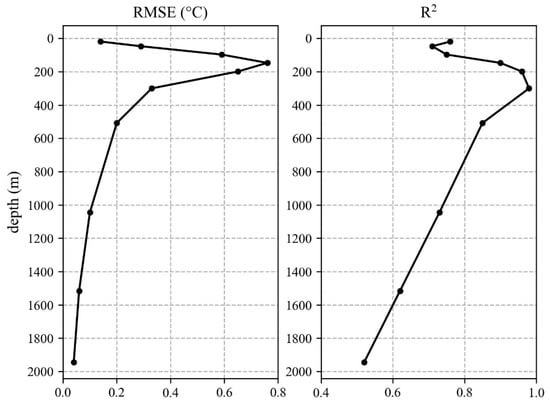
Figure 4.
Vertical profiles of errors from standard ConvLSTM method. (Left) is the RMSE and (Right) is R2.
Table 2.
Monthly RMSE and R2 of test sets from standard ConvLSTM method.
Overall, the accuracy of the direct retrieval from the sea surface data is reasonable but still needs improvement.
3.2. Results Retrieved from Improved Method with 50 m Layer’s Output as Input
We then made some changes to the models. We still configured and ran a model for every single layer. The models were still independent of each other. The configuration of the new models for the 20 and 50 m depth layers was similar to that of the standard ConvLSTM model, with only the sea surface anomaly data as input. After this, the retrieved temperature field from the 50 m layer model output, besides the sea surface anomaly data, was added as an input parameter into the ConvLSTM model training for each layer at the 100–500 m depths. The same 80% of the dataset as that selected for the work described in Section 3.1 was used as the training data, and the remaining 20% of the data were used for testing. The predictions were compared to the subsurface temperature data from CMEMS and the results from the standard ConvLSTM model by calculating the RMSE and R2.
Figure 5 illustrates a comparison of the errors between the standard ConvLSTM method and the improved method at the 100, 150, 200, 300, and 500 m layers. The trends of the RMSE and R2 are similar to those observed with the standard ConvLSTM method, with a maximum model error of 0.76 at the 150 m layer. The results indicate that the additional input improves the retrieval accuracy for deeper layers. It is most significant for the 100 m layer, where the RMSE is reduced by 12%, and the R2 is improved by 9%. We speculate that the reason for this result is that the water properties beneath the upper mixing layer (~100–200 m) do not vary simultaneously with the surface layer due to the differences in their dynamic forcing and mechanisms; rather, they correlate more with the layer in the middle, which is less exposed to surface external forcing. Table 3 shows the RMSE and R2 from this improved method for each month of the test set from the 100 to 500 m layers. In the 100 m layer, the RMSE increases and then decreases with the seasons, with a minimum error of 0.47 in the fall and a maximum error of 0.61 in the winter; in the 150 m layer, the RMSE increases with the seasons, with a minimum error in the spring and maximum error in the winter.
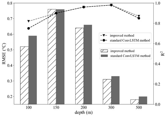
Figure 5.
Comparison of errors between standard ConvLSTM method and improved method. Bars represent the RMSE, and dashed lines represent R2.
Table 3.
Monthly RMSE and R2 of test sets from improved method.
The horizontal distributions of the temporally averaged RMSE at the 100–500 m depth layers from different methods are also compared and shown in Figure 6. For example, the error in Figure 6b improves significantly in the south, especially in the southwest region with the high error in Figure 6a. In Figure 6j, there is an east–west lateral high error region band at a 12°~15° N latitude, with the highest error in the region of 148°~152° E longitude; in Figure 6k, the high error region is significantly reduced. The right panel of Figure 6 (subplots c, f, i, l, o) shows the differences between the RMSE from the two methods. It can be seen that the values of the RMSE are reduced for almost all regions. The illustrations also imply that, for the regions where the errors are larger, the improved method decreases the magnitude of the errors, rather than reducing the area of the featured region. This phenomenon implies that the source of the error still exists, and the improved method does not fundamentally change the model but optimizes the result quantitatively.
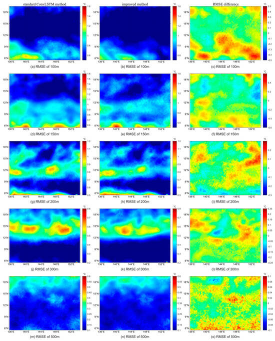
Figure 6.
Horizontal distributions of RMSE for different depth layers from standard ConvLSTM method (left) and improved method (center), and their differences (RMSE from standard ConvLSTM method minus that from improved method (right)).
4. Discussion
4.1. Pearson Correlation Coefficient Analysis
In our study, we designed the experiments based on the fact that the temperature structure of the 100–500 m depth layers is more correlative and varies more simultaneously with the “middle” layers, such as the 50 m layer, than with the surface layer. This is a precondition that distinguishes our work from a mathematical trick. Considering the modulation of the surface heat flux and wind forcing with regard to the temperature structure of the surface and near-surface layers, this assumption seems to be correct based on common sense, although it is difficult to explain directly from observations. In this section, we describe a simple test that we conducted to indirectly check the relationship between these layers.
In an attempt to prove this relationship, we calculated the Pearson correlation coefficients between the time series of the CMEMS temperature on each spatial point from the 0, 50, and 100–500 m layers, respectively. Figure 7 shows the spatially averaged values of these correlation coefficients. It can be seen from Figure 7 that the correlations between the surface temperature and 50 m temperature and the layers below them are reduced as the depth increases. Meanwhile, the correlation coefficients between the 50 m layer and the layers below are significantly higher than those between the surface and the same layers. The largest value of these correlation coefficients is that between the 50 and 100 m layers, which is as small as 0.47, suggesting the incapability of linear analysis tools in resolving the relationship between the surface and subsurface water temperature and the need to develop a deep learning method in this research field.
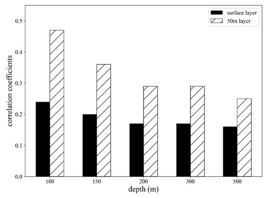
Figure 7.
Pearson correlation coefficients between the CMEMS temperature time series of surface and the layers below (black) and of 50 m and the layers below (diagonal lines).
4.2. Analysis of Significant Improvement at 100 m Layer
The vertical profile of the retrieved temperature’s RMSE features a peak in extreme large values at the 100–300 m depth. As shown in the left panel of Figure 8, the thermocline is located at this depth. The thermocline, undergoing complex dynamical processes and drastic changes in temperature, is usually located around this depth. The peak RMSE may be attributed to the vertical perturbation of the thermocline and the resulting drastic temperature variation. The RMSE is lower at the upper 50 m depth as the surface features are still influential at this depth; it is also lower below a 500 m depth since the distribution of the temperature does not vary much, as seen from the right panel of Figure 8. The decrease in the R2 with depths below the 500 m layer also suggests that the existence of the thermocline cuts off the impact of the surface features on the middle and deep seawater and makes it more challenging to predict the temperature structure at this depth with methods relying on only surface data. It is almost meaningless to retrieve the temperature structure under a 1000 m depth with AI methods such as ConvLSTM, since the retrieval RMSE and the temperature’s standard deviation are of similar magnitudes.
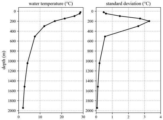
Figure 8.
Vertical profiles of water temperature (left) and its standard deviation (right) from CMEMS data.
In this study, we applied the improved method to the 100, 150, 200, 300, and 500 m layers, and the results showed a significant improvement only at the 100 m layer, with no notable improvement at the other layers. We still attribute these results to the vertical perturbation of the thermocline. The thermocline shifts seasonally and with climatologic events at the depth range of 100–300 m. For the 100 m layer, which is above the thermocline, the temperature structure undergoes similar physical processes to the 50 m layer, resulting in an obvious enhancement in the retrieval accuracy with the new method. However, for the 150, 200, and 300 m layers, the thermocline may lie above them at certain periods and below them at other periods. This uncertainty can render the new method ineffective. For the 500 m layer, which is below the thermocline, the new method performs equally poorly as the standard ConvLSTM method.
4.3. Possibility That Result Was Obtained by Chance
In our experiments, some of the data were randomly selected to create a training set, and the rest acted as a test set. It is shown in Table 2 and Table 3 that the RMSE features notable monthly variation, and the performance of the improved method varies from month to month. Considering that there are only 62 samples (data for 62 months) in the test set, i.e., five samples for each month on average, the results are greatly affected by whether the samples are from the months in which the new method performs well or poorly. Since the error reduction with the improved method is much smaller than the errors themselves in magnitude, there exists the possibility that the improvement in the method is attributed to the partition of the input data.
In order to further test whether the improvement observed with the new method arose by chance, a set of random tests was carried out by designing five different random seeds. Each random seed was used to select the training set from all input data for a test. The temperature at the 100 m layer was retrieved from both the standard ConvLSTM method and the improved method, respectively, for each test with a unique random seed. The error performance of all tests is shown in Table 4. It can be seen that the RMSE and R2 of the errors show similar relationships for the two methods in all cases, although their values vary with the cases. The result indicates that the improvement in the new method does not arise from the data selection.
Table 4.
RMSE and R2 values from the two methods in the test cases mentioned in Section 4.3.
5. Conclusions
In this study, the ConvLSTM model was employed to retrieve the three-dimensional temperature structure from multi-source sea surface parameters in the Western Pacific Ocean, with the CMEMS reanalysis temperature data serving as labeling and validation data for the retrieval. A new experimental workflow to increase the retrieval accuracy without additional input data was put forward.
The new experimental workflow takes the output of the 50 m layer model for the construction and training of the deeper layer’s model, considering the better correlation between the 50 m layer and the layers beneath it than that between the 0 m layer and these layers. This improved method resulted in an 11% decrease in the RMSE and a 9% increase in the R2 compared to the standard ConvLSTM method.
Although the improved method still has limitations, such as the fact that it only changes the retrieval errors quantitatively and does not modify their spatial distribution types, it would be beneficial to consider some non-mathematical factors when solving oceanographic problems with the deep learning method. In future research, we will try to introduce more physical and dynamic factors into the field of AI oceanography. Considering the inherent physical linkages between different types of marine parameters, the physics-driven perspective may have an effect on both aspects, namely increasing the accuracy and reducing the consumption, and it should not be ignored in the research field of data-driven marine science.
Author Contributions
Conceptualization, Y.L. and P.H.; methodology, Y.Z. and Y.K.; software, Y.Z.; validation, Y.L.; formal analysis, Y.Z.; resources, Y.L.; data curation, Y.L.; writing—original draft preparation, Y.Z.; writing—review and editing, Y.L., Y.K. and P.H.; visualization, Y.Z.; supervision, P.H.; project administration, Y.L.; funding acquisition, Y.L. All authors have read and agreed to the published version of the manuscript.
Funding
This research was jointly funded by the National Key Research and Development Program of China, grant number 2022YFC2808304, and the National Nature Sciences Foundation of China, grant number 42176014.
Institutional Review Board Statement
Not applicable.
Informed Consent Statement
Not applicable.
Data Availability Statement
The data presented in this study are available on request from the corresponding author.
Conflicts of Interest
The authors declare no conflicts of interest.
References
- Roemmich, D.; Alford, M.H.; Claustre, H.; Johnson, K.; King, B.; Moum, J. On the future of Argo: A global, full-depth, multi-disciplinary array. Front. Mar. Sci. 2019, 6, 00439. [Google Scholar] [CrossRef]
- Roemmich, D.; Johnson, G.; Riser, S.; Davis, R.; Gilson, J.; Owens, W.B. The Argo program: Observing the global oceans with profiling floats. Oceanography 2009, 22, 34–43. [Google Scholar] [CrossRef]
- Klemas, V.; Yan, X.H. Subsurface and deeper ocean remote sensing from satellites: An overview and new results. Prog. Oceanogr. 2014, 122, 1–9. [Google Scholar] [CrossRef]
- Talley, L.D.; Pickard, G.L.; Emery, W.J.; Swift, J.H. Data analysis concepts and observational methods. In Descriptive Physical Oceanography, 6th ed.; Elsevier: London, UK, 2011; pp. 147–186. [Google Scholar]
- Chen, X.; Tung, K.K. Varying planetary heat sink led to global-warming slowdown and acceleration. Science 2014, 345, 897–903. [Google Scholar] [CrossRef]
- Meng, L.; Zhuang, W.; Zhang, W.; Yan, C.; Yan, X.H. Variability of the shallow overturning circulation in the Indian Ocean. J. Geophys. Res. Ocean. 2020, 125, C015651. [Google Scholar] [CrossRef]
- Yan, X.H.; Boyer, T.; Trenberth, K.; Karl, T.R.; Xie, S.P.; Nieves, V.; Tung, K.K.; Roemmich, D. The global warming hiatus: Slowdown or redistribution? Earth’s Future 2016, 4, 472–482. [Google Scholar] [CrossRef]
- Ali, M.M.; Swain, D.; Weller, R.A. Estimation of ocean subsurface thermal structure from surface parameters: A neural network approach. Geophys. Res. Lett. 2004, 31, 20308. [Google Scholar] [CrossRef]
- Wu, X.; Yan, X.H.; Jo, Y.H.; Liu, W.T. Estimation of Subsurface Temperature Anomaly in the North Atlantic Using a Self-Organizing Map Neural Network. J. Atmos. Ocean. Technol. 2012, 29, 1675–1688. [Google Scholar] [CrossRef]
- Su, H.; Wu, X.; Yan, X.H.; Kidwell, A. Estimation of subsurface temperature anomaly in the Indian Ocean during recent global surface warming hiatus from satellite measurements: A support vector machine approach. Remote Sens. Environ. 2015, 160, 63–71. [Google Scholar] [CrossRef]
- Su, H.; Huang, L.; Li, W.; Yang, X.; Yan, X.H. Retrieving Ocean Subsurface Temperature Using a Satellite-Based Geographically Weighted Regression Model. J. Geophys. Res. Ocean. 2018, 123, 5180–5193. [Google Scholar] [CrossRef]
- Cheng, H.; Sun, L.; Li, J. Neural Network Approach to Retrieving Ocean Subsurface Temperatures from Surface Parameters Observed by Satellites. Water 2021, 13, 388. [Google Scholar] [CrossRef]
- Su, H.; Zhang, T.; Lin, M.; Lu, W.; Yan, X. Predicting subsurface thermohaline structure from remote sensing data based on long-short-term memory neural networks. Remote Sens. Environ. 2021, 260, 112465. [Google Scholar] [CrossRef]
- Hochreiter, S.; Schmidhuber, J. Long short-term memory. Neural Comput. 1997, 9, 1735–1780. [Google Scholar] [CrossRef]
- Chapman, C.; Charantonis, A.A. Reconstruction of Subsurface Velocities from Satellite Observations Using Iterative Self-Organizing Maps. IEEE Geosci. Remote Sens. Lett. 2017, 14, 617–620. [Google Scholar] [CrossRef]
- Uitz, J.; Claustre, H.; Morel, A.; Hooker, S.B. Vertical distribution of phytoplankton communities in open ocean: An assessment based on surface chlorophyll. J. Geophys. Res. Ocean. 2006, 111, C08005. [Google Scholar] [CrossRef]
- Charantonis, A.A.; Badran, F.; Thiria, S. Retrieving the evolution of vertical profiles of Chlorophyll-a from satellite observations using Hidden Markov Models and Self-Organizing Topological Maps. Remote Sens. Environ. 2015, 163, 229–239. [Google Scholar] [CrossRef]
- Han, M.; Feng, Y.; Zhao, X.L.; Sun, C.J.; Hong, F.; Liu, C. A Convolutional Neural Network Using Surface Data to Predict Subsurface Temperatures in the Pacific Ocean. IEEE Access 2019, 7, 172816–172829. [Google Scholar] [CrossRef]
- Meng, L.; Yan, C.; Zhuang, W.; Zhang, W.; Yan, X.H. Reconstruction of three-dimensional temperature and salinity fields from satellite observations. J. Geophys. Res. Ocean. 2021, 126, C017605. [Google Scholar] [CrossRef]
- Shi, X.; Chen, Z.; Wang, H.; Yeung, D.Y.; Wong, W.K.; Woo, W. Convolutional LSTM network: A machine learning approach for precipitation nowcasting. In Proceedings of the 29th Annual Conference on Neural Information Processing Systems, Montreal, QC, Canada, 7–12 December 2015. [Google Scholar]
- Song, T.; Li, Y.; Meng, F.; Xie, P.; Xu, D. A Novel Deep Learning Model by BiGRU with Attention Mechanism for Tropical Cyclone Track Prediction in Northwest Pacific. J. Appl. Meteorol. Climatol. 2021, 61, 3–12. [Google Scholar] [CrossRef]
- Chang, L.; Xu, J.; Tie, X.; Wu, J. Impact of the 2015 El Nino event on winter air quality in China. Sci. Rep. 2016, 6, 34275. [Google Scholar] [CrossRef]
- Zhai, P.; Yu, R.; Guo, Y.; Li, Q.; Ren, X.; Wang, Y.; Xu, W.; Liu, Y.; Ding, Y. The strong El Niño of 2015/16 and its dominant impaction global and China’s climate. J. Meteorol. Res. 2016, 30, 283–297. [Google Scholar] [CrossRef]
- Kawamura, R. A Rotated EOF Analysis of Global Sea Surface Temperature Variability with Interannual and Interdecadal Scales. J. Phys. Oceanogr. 1994, 24, 707–715. [Google Scholar] [CrossRef]
- Pan, Y.H.; Oort, A.H. Global Climate Variations Connected with Sea Surface Temperature Anomalies in the Eastern Equatorial Pacific Ocean for the 1958–73 Period. Mon. Weather Rev. 1983, 111, 1244–1258. [Google Scholar] [CrossRef]
- Lanzante, J.R. Lag Relationships Involving Tropical Sea Surface Temperatures. J. Clim. 1996, 9, 2568–2578. [Google Scholar] [CrossRef][Green Version]
- Hsiung, J.; Newell, R.E. The Principal Nonseasonal Modes of Variation of Global Sea Surface Temperature. J. Phys. Oceanogr. 1983, 13, 1957–1967. [Google Scholar] [CrossRef]
- Anderson, D.L.T.; McCreary, J.P. Slowly Propagating Disturbances in a Coupled Ocean-Atmosphere Model. J. Atmos. Sci. 1985, 42, 615–630. [Google Scholar] [CrossRef][Green Version]
- Schopf, P.S.; Suarez, M.J. Vacillations in a Coupled Ocean–Atmosphere Model. J. Atmos. Sci. 1988, 45, 549–566. [Google Scholar] [CrossRef]
- Hurrell, J.W. Decadal trends in the North Atlantic oscillation: Regional temperatures and precipitation. Science 1995, 269, 676–679. [Google Scholar] [CrossRef]
- Ashok, K.; Behera, S.K.; Rao, S.A.; Weng, H.; Yamagata, T. El Nino Modoki and its possible teleconnection. J. Geophys. Res. 2007, 112, C11007. [Google Scholar] [CrossRef]
- Zhou, S.; Xie, W.; Lu, Y.; Wang, Y.; Zhou, Y.; Hui, N.; Dong, C. ConvLSTM-Based Wave Forecasts in the South and East China Seas. Front. Mar. Sci. 2021, 8, 680079. [Google Scholar] [CrossRef]
- Yao, L.; Wang, X.; Zhang, J.; Yu, X.; Zhang, S.; Li, Q. Prediction of Sea Surface Chlorophyll-a Concentrations Based on Deep Learning and Time-Series Remote Sensing Data. Remote Sens. 2023, 15, 448. [Google Scholar] [CrossRef]


Disclaimer/Publisher’s Note: The statements, opinions and data contained in all publications are solely those of the individual author(s) and contributor(s) and not of MDPI and/or the editor(s). MDPI and/or the editor(s) disclaim responsibility for any injury to people or property resulting from any ideas, methods, instructions or products referred to in the content. |
© 2024 by the authors. Licensee MDPI, Basel, Switzerland. This article is an open access article distributed under the terms and conditions of the Creative Commons Attribution (CC BY) license (https://creativecommons.org/licenses/by/4.0/).