Investigating Fishing Vessel Hydrodynamics by Using EFD and CFD Tools, with Focus on Total Ship Resistance and Its Components

Abstract

The aim of this work is to gain a better understanding of the hydrodynamics of a typical Argentinian fishing vessel in calm water. It is focused on the evaluation of total ship resistance and its components for different draughts. The 1978 ITTC Power Prediction method is used to predict total ship resistance from experiments carried out at the University of Buenos Aires towing tank. To conduct a more detailed evaluation of the flow around this hull, numerical studies at model scale are carried out with the open-source code OpenFOAM V10 and validated against experimental results. The Reynolds-Averaged Navier–Stokes (RANS) method together with Volume of Fluid (VOF) are used for the numerical procedure. The validated CFD model not only can provide more detailed information about the ship’s hydrodynamics than the EFD results but also allows for the exploration of the improvement in ship power prediction by using combined CFD-EFD methodologies. This work numerically calculates the form factor by using a double-body configuration and discusses the possibility of combining EFD results with this CFD form factor in order to improve total force prediction for this kind of ships.

1. Introduction

When a new vessel is commissioned, one of the most stringent criteria is to maintain the contract speed throughout its operational life. Any significant deviation from this specified speed at delivery could potentially lead to contract termination, presenting a dilemma for designers. Such deviations in propulsion could have a profound effect on various facets of the vessel’s operation, including operational efficiency, stability and, ultimately, profitability. Consequently, the determination of the speed–resistance curve becomes a critical consideration in ship design.

In the early stages of design, when the hull shape is largely defined, conventional approaches typically involve the use of statistical and regression methods. Holtrop and Mennen (1984) pioneered a regression technique based on extensive sea trials and over 200 model tests in towing tanks which has since become a staple for estimating ship resistance [1]. However, this method tends to produce higher uncertainties than results derived from Experimental or Computational Fluid Dynamics (CFD) analyses. For example, Bilec et al. (2020) demonstrated differences in resistance estimates of up to 30% when comparing Holtrop–Mennen predictions with experimental results for fishing vessels [2].

As ship design progresses, there is a need for more robust and accurate methods to account for various effects overlooked by statistical approaches. Experimental Fluid Dynamics (EFD) with towing tank tests is the preferred method by shipyards and owners and remains the gold standard for performance prediction due to its reliability. By extrapolating model-scale drag data, it is possible to anticipate full-scale performance requirements, a process commonly referred to as drag extrapolation.

Although the effectiveness of towing tank testing and extrapolation methods has been extensively discussed and refined over decades, inherent limitations due to scale effects remain. Model tests are performed to achieve Froude number similarity, but simultaneous Reynolds similarity remains a challenge.

As an alternative to towing tank testing, Computational Fluid Dynamics (CFD) has gained prominence for its ability to satisfy both Froude and Reynolds similarity while providing detailed insights into the flow. Over the past few decades, the use of CFD methods based on the Navier–Stokes equations has increased dramatically [3,4]. This development has facilitated the improvement of techniques and procedures for the accurate prediction of ship resistance on a model scale. However, concerns remain regarding the accuracy of CFD in predicting full-scale performance [5].

Recognising the potential of a combined approach, the ITTC Combined CFD-EFD Methods Specialist Committee advocates the use of both EFD and CFD to improve performance predictions. The integration of these methods is proposed to potentially reduce uncertainties introduced during model testing or extrapolation, thereby improving accuracy [6].

This study aims to deepen our understanding of the hydrodynamics of typical Argentine fishing vessels in calm waters. Specifically, we focus on evaluating the total ship resistance and its components under varying draughts. By using the 1978 ITTC Power Prediction method, we predict total ship resistance based on model-scale experiments conducted at the University of Buenos Aires towing tank. In addition, we perform model-scale numerical investigations by using the open-source code OpenFOAM, validated against experimental results. The Reynolds-Averaged Navier–Stokes (RANS) method coupled with Volume of Fluid (VOF) is used for the numerical simulations. We analyse the pressure distributions on the hull and the wave patterns under different loading conditions, with a focus on informing future hull optimisation efforts.

The validated CFD model not only provides more detailed hydrodynamic insights than the EFD results but also facilitates the refinement of ship performance predictions through combined CFD-EFD methods. Given the importance of the form factor in reducing uncertainties in the 1978 ITTC Power Prediction method, we numerically calculate the form factor by using a double-body configuration. Furthermore, we explore the potential of CFD-based form factors as an alternative or complement to Prohaska’s method for such vessels [7,8,9,10,11,12].

Understanding the behaviour of this type of vessel and improving performance prediction capabilities is critical in the evolving landscape of the Argentine shipbuilding industry. The Argentine fishing industry has undergone significant changes since the 1960s, marked by advances in vessel types and fishing methods [13]. Efforts to modernise the fleet and adopt sustainable technologies underline the importance of studies such as this in optimising the hydrodynamics of the vessels concerned.

The paper is structured as follows: Section 2 provides a description of the model and full-scale ship, together with details of the towing tank and an uncertainty analysis of the resistance tests. Section 3 describes the numerical model and procedure.

In Section 4, we present the comparison between EFD and CFD results for total resistance and wave patterns. In addition, we analyse the numerically obtained hull pressure distribution and examine the form factor derived from EFD and CFD to decompose the forces. Finally, we discuss the implications of the uncertainty in the form factor on the extrapolation process used to determine total resistance. Section 5 concludes the thesis by summarising the main findings.

2. Experimental Setup

As highlighted in the introduction, the quantification of ship resistance is a fundamental aspect of ship design. Typically, this is achieved by towing tank experiments, from which the ship’s resistance–velocity curve is derived. Total resistance measurements were performed over a range of Froude numbers (Fn) from 0.10 to 0.45.

2.1. Model and Full-Scale Ship

A typical Argentinian fishing vessel was chosen for this study. The model was constructed at a scale of $\lambda$ = 20 by using glass fibre-reinforced plastic (GFRP), following the ITTC-recommended procedure [14]. Two 1.0 mm diameter tripwires were used to induce turbulence. One was positioned downstream of the forward perpendicular at a distance equal to five percent of $L_{WL}$. The other was placed downstream of the front end of the bulb at a distance equal to one-third of the bulb length.

Table 1. Main parameters of full-scale ship and ship model.

Main Particulars	Symbol	Unit	Full Scale	Model	Model	Model
			T1	T1	T2	T3
Model scale	$\lambda$	[-]	-	20	20	20
Length on waterline	LWL	[m]	32.68	1.634	1.662	1.641
Length, overall submerged	LOS	[m]	34.795	1.670	1.740	1.740
Breadth	B	[m]	9.28	0.464	0.464	0.464
Draught	T	[m]	3.30	0.165	0.180	0.195
Displacement volume	∇	[m3]	599.40	0.075	0.085	0.095
Wetted surface area	S	[m2]	392.67	0.982	1.058	1.124
Block coefficient	CB	[m]	0.60	0.60	0.61	0.64
Midship section coefficient	CM	[m]	0.86	0.86	0.87	0.89

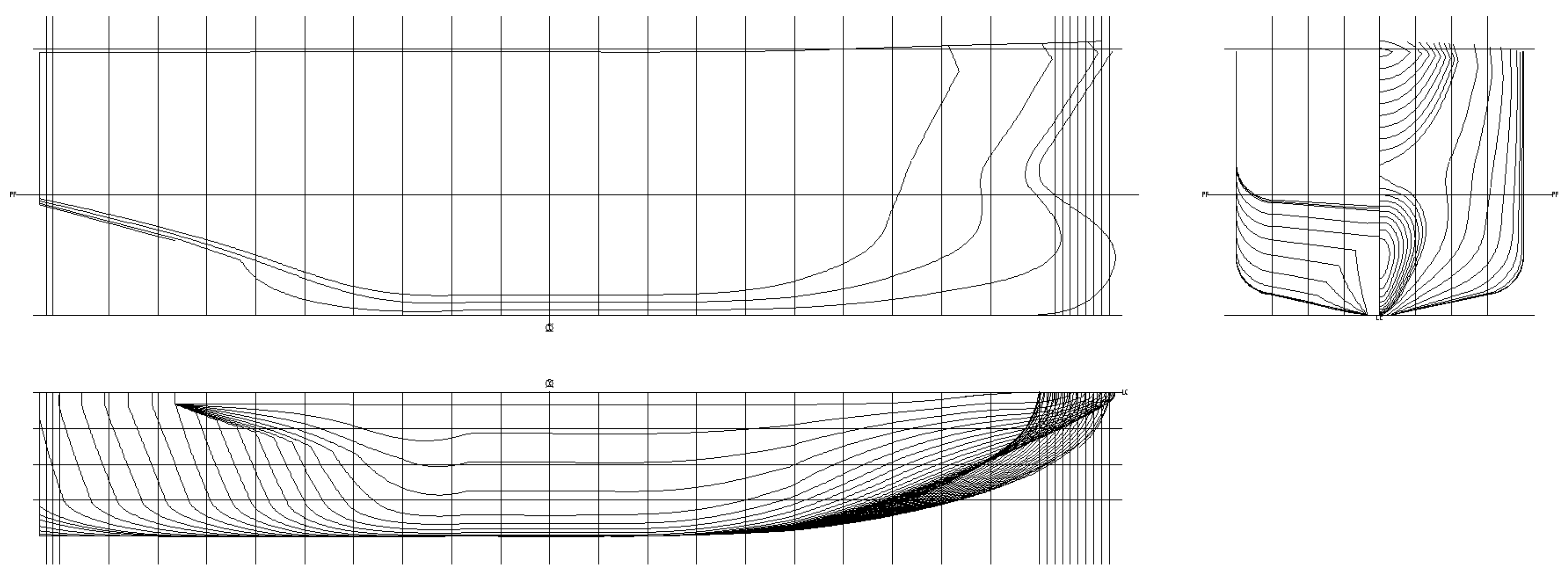
shows the main characteristics of both the full-scale ship and the model. Three loading conditions (LCs) were studied: ballast (T1), intermediate loading (T2) and full loading (T3). The main characteristics of the full-scale ship are given for reference purposes only for the ballast condition (T1). Figure 1 shows the body lines of the hull.

2.2. Towing Tank

The experimental tests were carried out in the towing tank of University of Buenos Aires (UBA), Argentina, known as Canal de Experiencias de Arquitectura Naval (CEAN). The tank is 72 m long, 3.6 m wide and 2 m deep.

Equipped with a trolley capable of reaching a maximum speed of 4.0 m/s, the towing tank facilitated the experiments. The model, ballasted to the required displacement and waterline, was mounted on the load cell. A single-component load cell, specifically Kempf & Remmers model R 47, was used for the resistance tests. Coupling the model to the trolley via the load cell ensured that heave, yaw and roll were eliminated, allowing the model to be free to trim and sink. The resistance transducer, designed for a full-scale load of ±100 N, has a sensitivity of approximately ±1 mV/V of supply voltage.

The mean cross-sectional area of the ship represents 1%, 1.1% and 1.2% of the towing tank cross-sectional area under light-, medium- and heavy-load conditions, respectively. The Schuster blockage correction method was, therefore, applied in accordance with the ITTC procedure [15].

2.3. Uncertainty Analysis Resistance Tests

Uncertainty analysis for drag measurement requires the consideration of all significant components of uncertainty associated with total drag. These include uncertainties associated with hull geometry, towing speed, water temperature, dynamometer calibration and replicate testing. These standard uncertainty components are estimated and then combined to give the total standard uncertainty by using the Root Sum Squares (RSS) method as recommended by the ITTC [16].

The total resistance of a hull model at a given Froude number (Fn) is a function of the wetted surface area of the hull and the Reynolds number (Re), assuming that the geometry uncertainty in a ship model hull does not normally affect the residual resistance coefficient. The uncertainty components of the wetted surface area and the representative length of the model can be estimated in terms of the standard uncertainty in the displacement mass. Finally, the uncertainty in the hull geometry is quantified by measuring the model ballast. The model and the weights used to ballast the model were weighed by using a portable beam scale. The resulting uncertainties on the hull geometry are presented in the

Table 2. Combination of uncertainty in resistance measurements at Fn = 0.14, Fn = 0.26 and Fn = 0.37. Repeat test N = 4.

Uncertainty Components	Fn = 0.14	Fn = 0.26	Fn = 0.37
Hull geometry	0.05	0.05	0.05
Speed	0.067	0.067	0.067
Water temp.	0.03	0.03	0.03
Dynamometer	4.73	1.04	0.35
Repeat test, deviation a	5.00	3.50	1.50
Combined for single test	6.88	3.65	1.54
Repeat test, deviation of mean	2.50	1.75	0.75
Combined for repeat mean	5.35	2.04	0.83
Expanded for repeat mean	10.70	4.08	1.66

[^a] Repeat test, Deviation = (Repeat test, Deviation of mean) ∗ ${\mathrm{N}}^{1/2}$.

for speeds of Fn = 0.14, Fn = 0.26 and Fn = 0.37.

The uncertainty in towing speed is propagated into the drag measurement through the dynamic pressure and the Reynolds number. The relative uncertainty in towing speed is considered the bias limit of the towing vehicle. The resulting uncertainties in drag due to speed are given in Table 2.

Variations in water temperature have a significant effect on water viscosity and consequently on the Reynolds number and frictional drag of the hull model. Throughout the tests, the water temperature varied by less than 0.5 °C. The corresponding uncertainties in drag due to temperature variations are shown in Table 2.

The dynamometer was calibrated before and after each test. A linear curve fit was used, and the standard deviation of this linear regression was taken as the standard uncertainty in calibration. The accuracy of the weights was sufficiently high that their uncertainty was negligible. The corresponding uncertainties in the calibration of the dynamometer are given in Table 2.

By using the R47 dynamometer to measure resistance at a sampling rate of 200 Hz, the measurement at each speed was obtained by averaging the time history of the signal from the data acquisition system (DAS) over a time interval of at least 10 s. The load cell signal was low-filtered at 4 Hz before reaching the DAS. The standard uncertainty in the average of the sampling history ranged from 0.0007% to 0.003%, with the average of all replicates being 0.0012%. Consequently, the uncertainty of a reading from the DAS was considered negligible.

The mean of the repeated resistance measurements was taken as the best estimate. The standard uncertainty component of the mean of N replicate tests was estimated according to the ITTC procedure [16]. The standard uncertainties for replicates with N = 4 are given in Table 2.

Finally, the significant components of the uncertainties were combined by the RSS (Root Sum Square) method and are presented in Table 2.

As can be seen in Table 2, the dynamometer and the precision of the measurement were the main sources of uncertainty due to repeated testing. The uncertainty in resistance measurements for Fn = 0.14, Fn = 0.26 and Fn = 0.37 were 5.35%, 2.04% and 0.83%, respectively. The uncertainty decreases with the increase in speed because the contribution from the dynamometer decreases at higher speeds. The expanded uncertainties in Table 2 correspond to a confidence level of 95%.

3. CFD Model

3.1. Numerical Methods

In the field of naval engineering, Computational Fluid Dynamics (CFD) is emerging as a key tool, especially for the assessment of resistance. Among the many codes available, OpenFOAM stands out as a widely used platform, chosen for its versatility and its adherence to the finite volume method. This open-source software facilitates the implementation of the Navier–Stokes equations, as well as various numerical schemes and turbulence models. Throughout the study, OpenFOAM played a crucial role in mesh generation and solving the governing equations. In addition, Rhinoceros was used for geometry generation and Paraview for visualisation of the results.

When numerically calculating the ship’s resistance, the governing equations must encapsulate Newtonian, turbulent, incompressible and viscous flow characteristics. The Navier–Stokes equations, which include mass (1) and momentum (2) considerations, form the cornerstone. The Reynolds-Averaged Navier–Stokes (RANS) method, specifically the SST k-$\mathsf{\omega }$ model, has been used to treat turbulence. This model, with two eddy viscosity equations, has been shown to be effective in previous studies [17].

Simulations were carried out for both single-fluid and two-phase scenarios. For single-fluid simulations, the above equations were sufficient. However, for scenarios involving air and water phases, the Volume of Fluid (VOF) method became indispensable. This method, governed by Equation (3), distinguishes between the two fluids using a scalar volume fraction $\alpha$, where $\alpha$ ranges between 0 and 1 and represents the proportion of each phase within a given fluid cell.

Furthermore, the comparative CFD analyses between the free-heave and -pitch cases and the constrained cases (fixed sinkage and trim) showed minimal discrepancies. The test was carried out at Fn = 0.4 for the T3 draught, expecting big changes due to a bigger projected area exposed to fluid pressure, but the differences in the calculated drag values did not exceed 1.5%. So, although trim and heave were monitored during the towing tank tests, ship attitude comparisons were not performed in conjunction with the CFD simulations due to the fixed-heave and -trim configurations aimed at computational efficiency.

$$\nabla ·\overline{U_f}=0$$

(1)

$$\frac{\partial \left({\rho }_f\overline{U_f}\right)}{\partial t}+\nabla \left({\rho }_f\overline{U_f}\overline{U_f}\right)={\rho }_{f}g-\nabla p+{\mu }_f{\nabla }^2\overline{U_f}$$

(2)

$$\frac{\partial \left(\alpha \right)}{\partial t}+\overline{U_f}·\nabla \alpha =0$$

(3)

3.2. Numerical Domain and Boundary Conditions

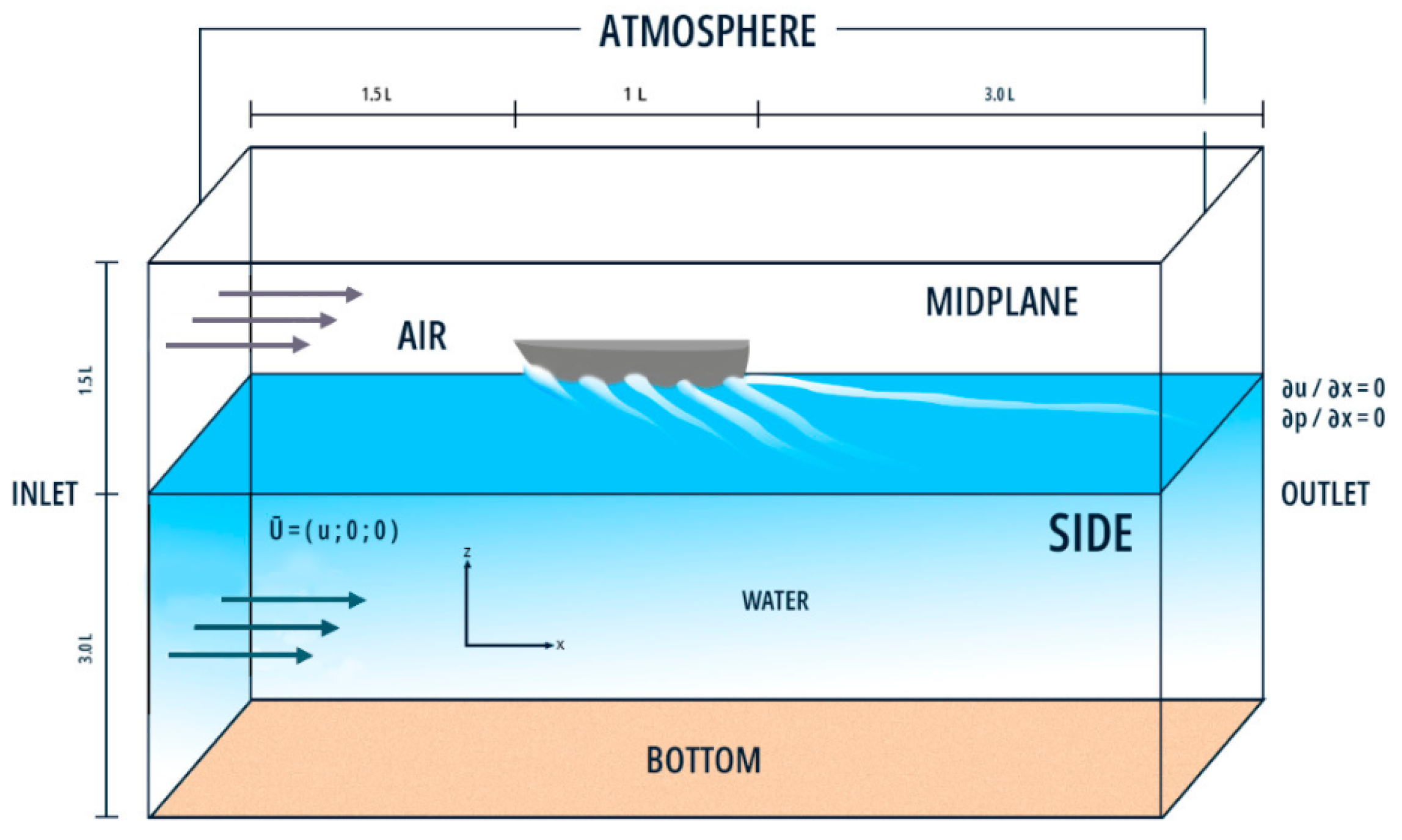
The computational domain to be used is shown in Figure 2. The distances within the domain were carefully chosen to ensure sufficient distance from the hull model to mitigate any blockage effects. The boundary conditions used are outlined in

Table 3. Boundary conditions.

Patch	U	p	k	$\mathit{\omega }$	$\mathit{\mu }$ Turbulent
-	m/s	kg/m$·$s2	m2/s2	1/s	m2/s
Inlet	Uniform	Fixed flux	Fixed value	Fixed value	Fixed value
Outlet	Zero grad	Zero grad	Zero grad	Zero grad	Zero grad
Atmosphere	Zero grad	Zero grad	Zero grad	Zero grad	Zero grad
Bottom	Symmetry	Symmetry	Symmetry	Symmetry	Symmetry
Midpl/side	Symmetry	Symmetry	Symmetry	Symmetry	Symmetry
Ship	No slip	Fixed flux	Wall function	Wall function	Wall function

.

Turbulent variables such as k and $\mu$ were set to fixed values close to 0 in all cases to mimic the laminar conditions at the towing tank. The SST k-omega model can correctly handle the turbulence generation around the hull when the flow surrounds the latter.

3.3. Mesh Convergence

The criterion chosen for the mesh convergence analysis was the direct comparison between the experimental and computational drag at Fn = 0.45 for T1 = 0.165 m. Various mesh configurations were evaluated, systematically refining the cell size within the central region by a factor of 1.2. The results, detailed in

Table 4. Mesh convergence analysis.

Case	Mesh Cells	Fn	F [N]	Error (%)
EFD	-	0.45	40.27	-
Mesh 1	633.938	0.45	40.26	0.02
Mesh 2	903.744	0.45	41.76	3.70
Mesh 3	1.213.419	0.45	40.34	0.17
Mesh 4	2.485.166	0.45	41.16	2.21

, show an oscillatory convergence pattern across the meshes tested.

Despite slight variations, all configurations show errors below 4%, indicating acceptable accuracy. Subsequent simulations were performed using a first-order pseudo-transient time scheme with a tailored local time step, eliminating the need for further numerical sensitivity evaluations. The robustness of the numerical setup was confirmed. This mesh was used exclusively for resistance tests over the entire Fn range, but not for the double-hull method. In cases where the double-hull approach was required for form factor determination, the ITTC Grid Convergence Index was used to ensure grid independence as mentioned in Section 4.4.

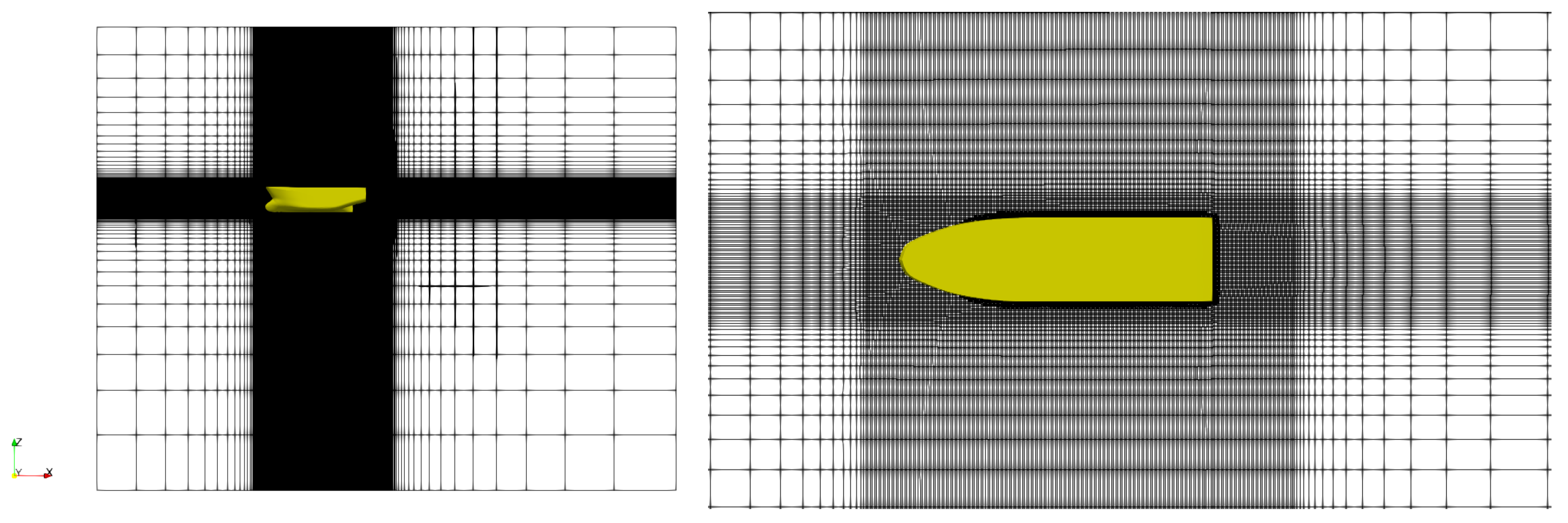
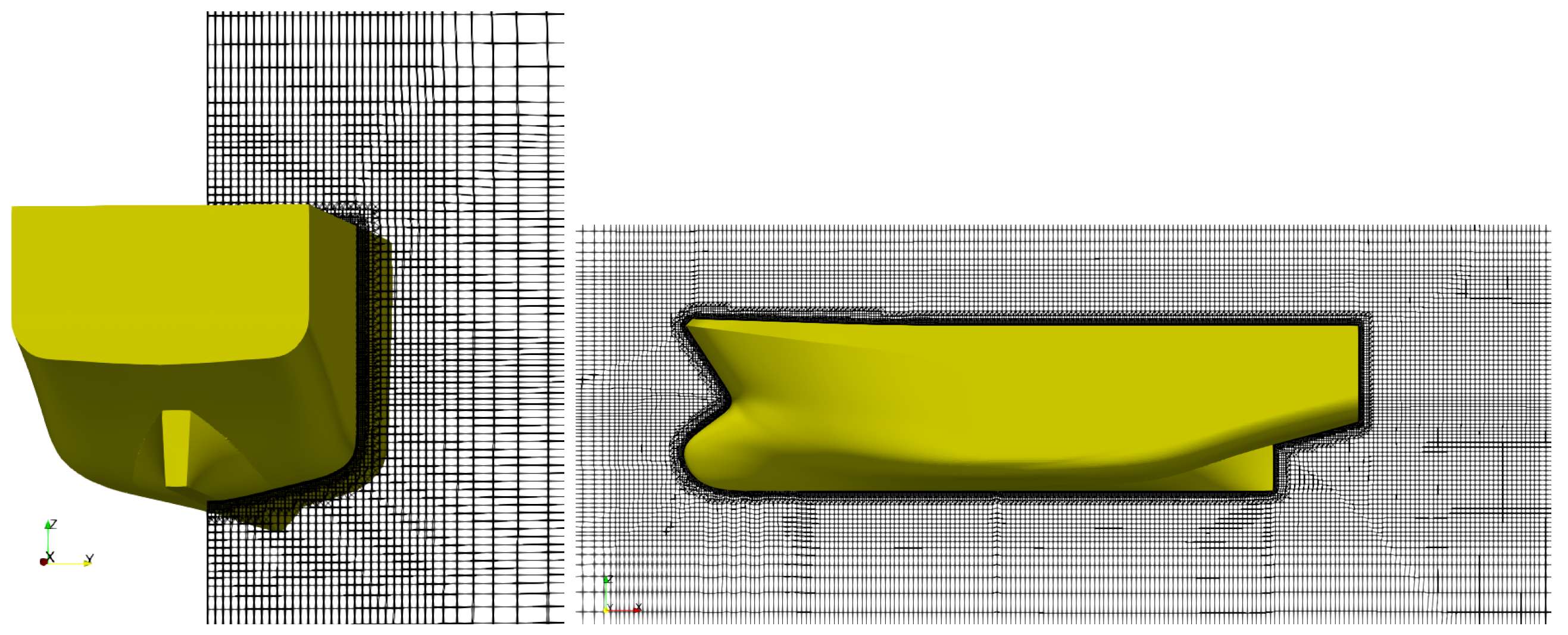
Figure 3 and Figure 4 illustrate the resulting mesh configuration, characterised by horizontal expansion ratios of 1.3 and 1.2 along the x- and y-axes, respectively, together with a vertical expansion ratio of 1.2, all converging towards the central zone. The vessel was enclosed within a block composed primarily of hexahedrons with an aspect ratio of one, except in the interface zone, where cell heights were reduced by 25% to accurately capture wave characteristics. The mesh design prioritises maintaining a y+ value below 5 in all scenarios. To achieve this, the snappyHexMesh layers tool was used to surround up to 98% of the hull surface with prismatic layers. The chosen wall function ensures that the correct function is used according to the y+ value found, whether it is in the viscous or logarithmic sublayers.

For the cases with a double hull, the same mesh was used for the lower part of the domain. The top boundary was set at the different draught lines with a symmetry condition for every variable.

4. Results

4.1. EFD and CFD Total Resistance Curve and Wave Pattern

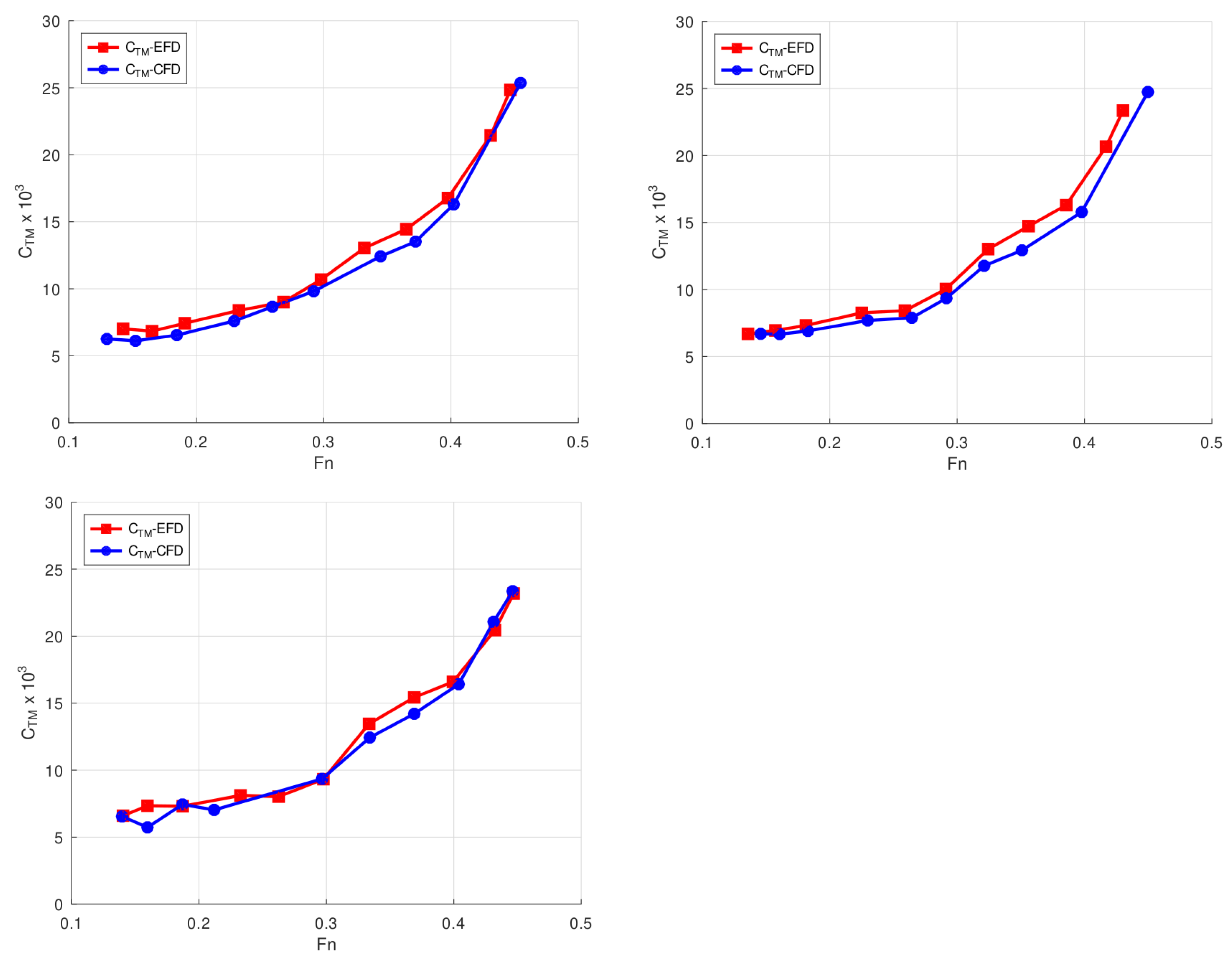
In this subsection, the EFD total resistance curve is analysed and compared with the CFD curve. Figure 5 shows the EFD and CFD dimensionless total resistance curve ($C_{TM}$) versus Froude number (Fn) considering different draughts. The coefficient $C_{TM}$ is defined as follows:

$$C_{TM}=\frac{R_{TM}}{\frac{1}{2}\rho S_M{V_M}^2}$$

(4)

where $R_{TM}$ is the model total resistance, $V_M$ is the model velocity, $\rho$ is the water density and $S_M$ is the model wetted surface area. A good agreement in $C_{TM}$ between EFD and CFD results is observed for the three investigated flows and the different Froude numbers.

Normally, fishing vessels operate under different conditions and thus at different speeds and draughts, for example, when the vessel leaves port to fish, when it fishes and also when it returns to port with the catch. Usually, the design criteria are based on the speed in the phases of moving towards the fishing area and the return to port with the catch. In the present case, the vessel was designed to travel at 0.25 < Fn < 0.45, where the defined operating speed was Fn = 0.35. Therefore, the ship was considered a displacement ship according to [18]. The curves show the typical behaviour for this type of ship. Figure 5 also shows that for low speeds (Fn < 0.3), the total drag is almost equal to the viscous drag and $C_{TM}$ increases almost linearly.

For higher Fn, the slope of the total resistance curve increases continuously, indicating that $C_{TM}$ increases at a rate greater than the square of the model ship’s speed. Wave resistance is negligible at low speeds, but as speed increases, wave resistance grows faster than viscous resistance. In fact, for most fishing vessels, above Fn = 0.30, wave resistance becomes the largest component of their resistance, abruptly increasing the total ship resistance and thus, in some cases, making vessels inefficient from a consumption point of view.

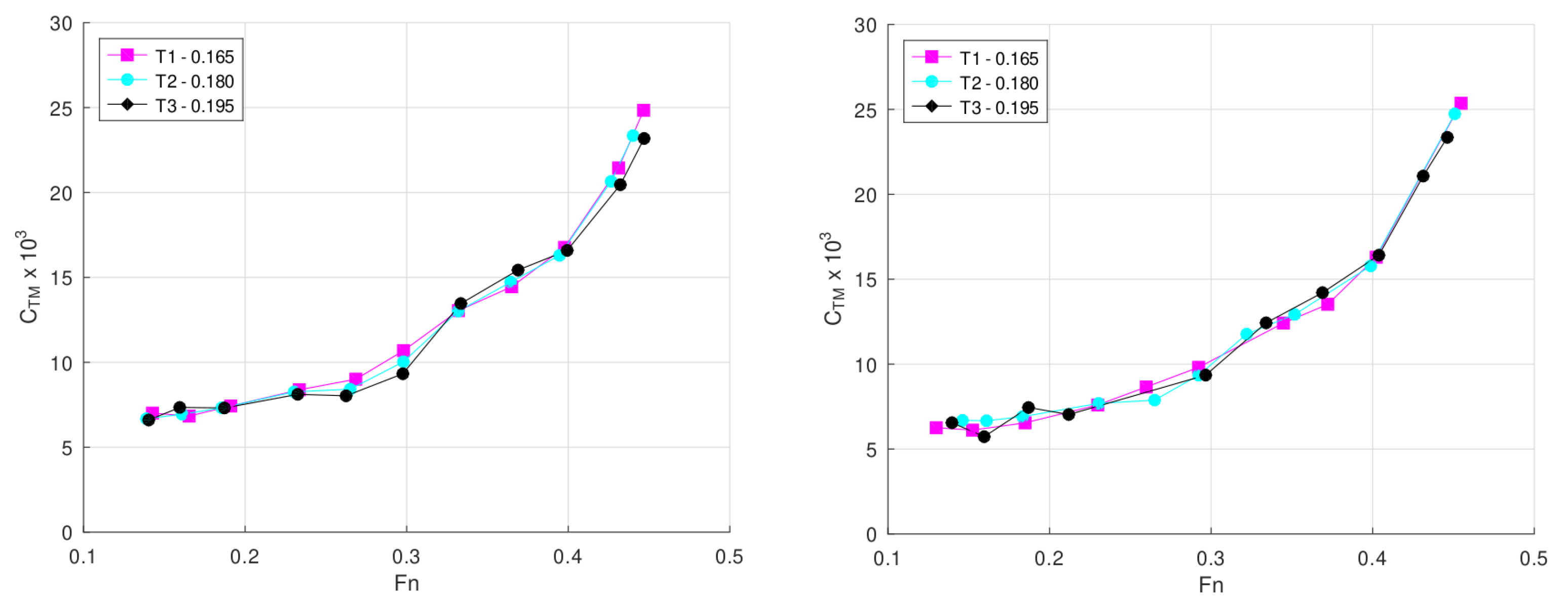
Figure 6 shows the $C_{TM}$-versus-Fn curves separately for EFD and CFD to emphasise the influence of draught on $C_{TM}$. The left graph shows the EFD drag results for different draughts, while the right graph shows the CFD model results.

As expected, the EFD results indicate that for Fn < 0.3, draught changes do not result in significant changes in total ship resistance. At such low Fn values, resistance increases as the wetted surface area of the hull increases. However, these variations in $C_{TM}$ are not visible in Figure 6 due to the very low resistance values in this Fn range. Conversely, draught effects become noticeable for 0.3 < Fn < 0.40. In this interval, although wave resistance becomes the dominant component, viscous resistance still contributes significantly to the total resistance, resulting in an increase in $C_{TM}$ with the increase in draught. Finally, for Fn > 0.4, all curves tend to converge to a similar value due to the significant increase in wave resistance, which masks the draught effect and hence the viscous resistance.

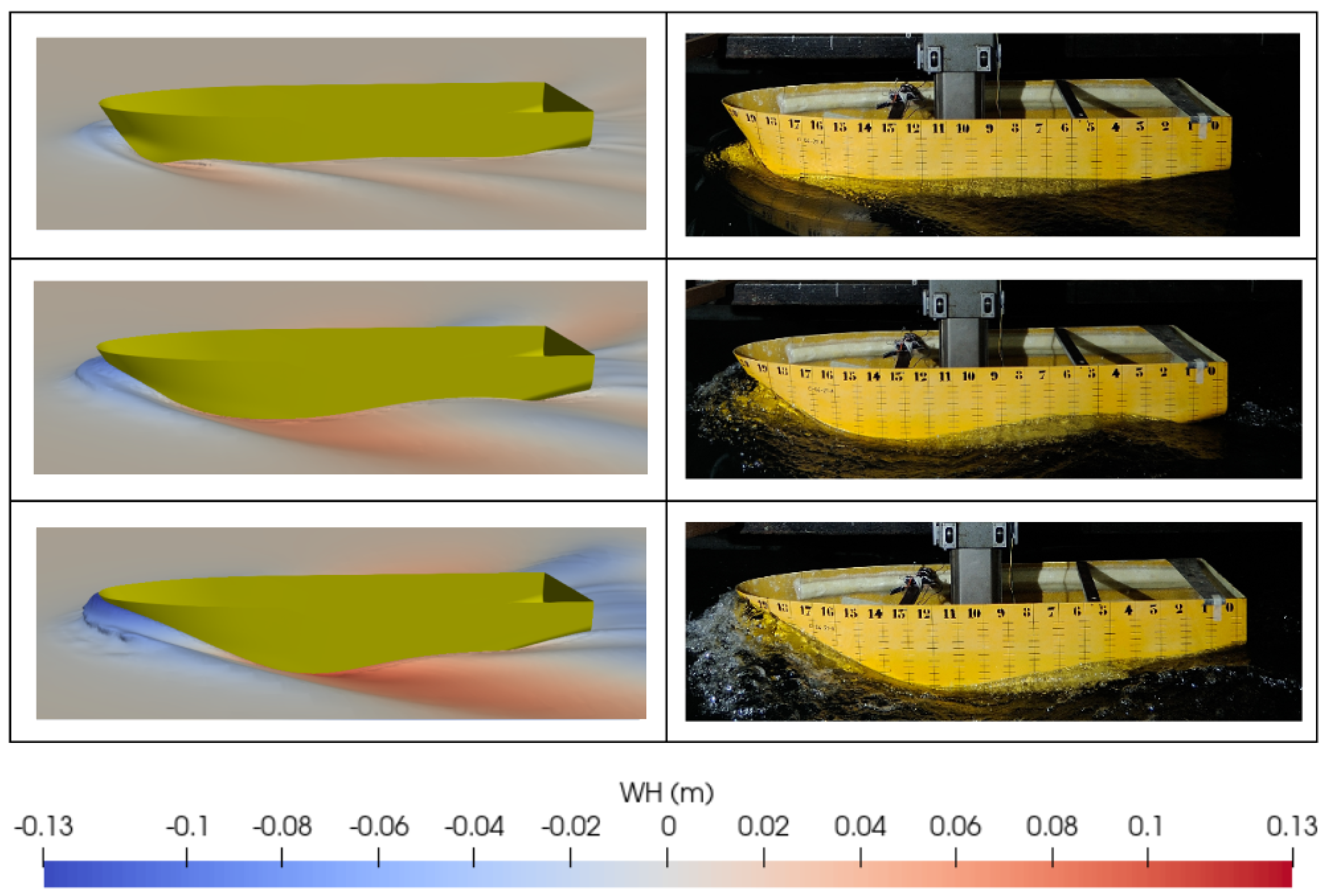
From the above observations, it is clear that wave resistance plays a crucial role in assessing the performance of this type of fishing vessel. Therefore, understanding the wave pattern across the hull of a vessel is essential to designing and operating efficient vessels. Figure 7 shows a comparison of the wave pattern distribution along the hull obtained with the CFD model and EFD, for draught T3 with different Fn values. The three cases illustrate the ability of the CFD model to reproduce the wave pattern generated by the ship for different Fn values.

In ship hydrodynamics, it is common to divide wave resistance into two components: wave pattern resistance and wave breaking resistance. If Fn is sufficiently high, waves can become steep enough to break into eddies and spray. The energy removed from the wave system is then found in the ship’s wake and constitutes the wave breaking resistance. The remaining wave energy is radiated away from the ship through the wave system, giving rise to wave pattern resistance. The breaking phenomenon can be seen in the EFD results for Fn > 0.3 (Figure 7, second row for Fn = 0.37 and third row for Fn = 0.45).

The CFD results capture the wave breaking phenomenon only for the highest Fn number (Figure 7, third row for Fn = 0.45). A more detailed description of this phenomenon with the CFD model would require a finer mesh in the interface region. However, it is important to note that the wave breaking resistance is much smaller than the wave pattern resistance for this type of fishing vessel. The hull shoulders play an important role in wave generation and distribution along the hull. It is worth noting that for higher Froude numbers, a maximum hollow wave occurs at hull section 14.5 and moves backwards to about section 11.5 for Fn = 0.45.

4.2. CFD Pressure Distribution

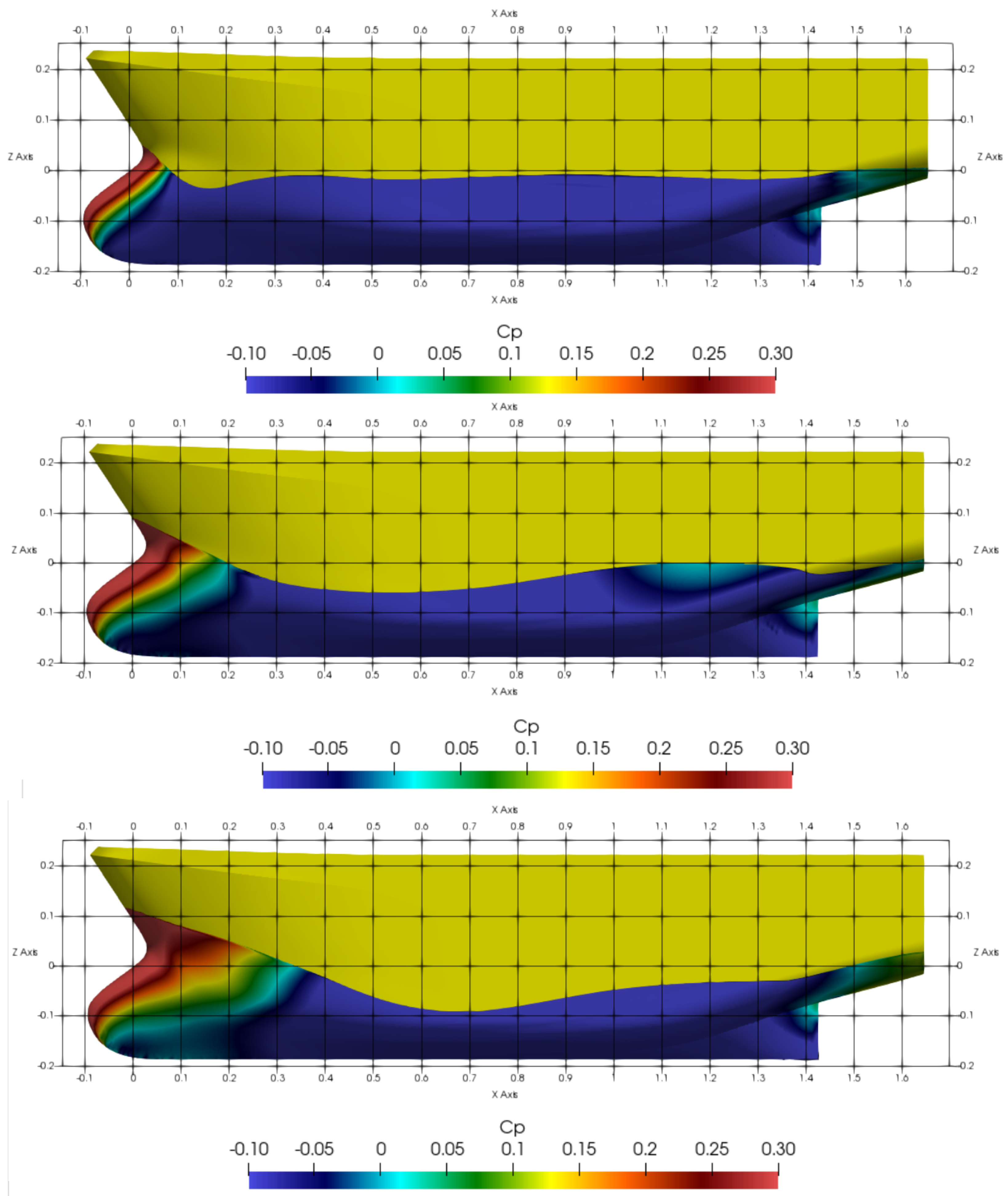
The validation of the CFD model allows for the determination of variables that would be difficult to obtain by using EFD techniques. For example, directly related to the wave resistance phenomenon is the pressure distribution on the hull. Figure 8 shows the dimensionless pressure distribution ($C_P$) on the hull for different Fn values at T3. This dimensionless parameter is defined as

$$C_P=\frac{p-p_{\infty }}{\frac{1}{2}\rho {V_M}^2}$$

(5)

where $p-p_{\infty }$ is the dynamic pressure.

The pressure distribution over the hull of a ship plays a key role in determining its wave generation and resistance characteristics, as these pressures can be thought of as a series of perturbations propagating outwards from the hull. These pressure distributions determine the shape and magnitude of the waves generated. As shown in Figure 8, high- and low-pressure zones coincide with wave crests and troughs.

In general, a smooth and even pressure distribution across the hull results in a more efficient and less resistant movement through water. This is because an even pressure distribution creates fewer disturbances in the water, resulting in less energy lost to wave generation and less drag on the vessel. Conversely, an uneven pressure distribution can create more disturbance in the water, leading to increased wave generation and resistance. Such uneven distributions can occur if the hull shape is not optimised for the vessel’s speed and operating conditions.

Understanding and managing the distribution of pressure across a ship’s hull is, therefore, crucial to designing and operating ships that are both efficient and effective.

4.3. Experimental Form Factor Determination

The ITTC method of splitting the total drag coefficient incorporates Hughes’ hypothesis [19] and introduces the form factor k to augment the flat plate drag coefficient ($C_F$). This enhancement accounts for the Reynolds number-dependent viscous drag and the shape effects on the boundary layer itself [15].

$$C_T=(1+k)C_F+C_W$$

(6)

Once a form factor k has been determined, the wave resistance coefficient ($C_W$) is obtained by solving the following equation:

$$C_W=C_{TM}-(1+k)C_{FM}$$

(7)

where $C_{FM}$ is the ITTC-57 correlation line coefficient for the Reynolds number of the model test and $C_{TM}$ is the dimensionless total resistance of the model ship. Prohaska [7] proposed a method for determining the form factor from model tests which is considered to be the most reliable method available. It assumes that for Fn < 0.2, $C_W$ can be approximated by $\alpha$Fn⁴. So, Equation (6) for the model can be rewritten as

$$\frac{C_{TM}}{C_{FM}}=(1+k)+\alpha \frac{F{n}^4}{C_{FM}}$$

(8)

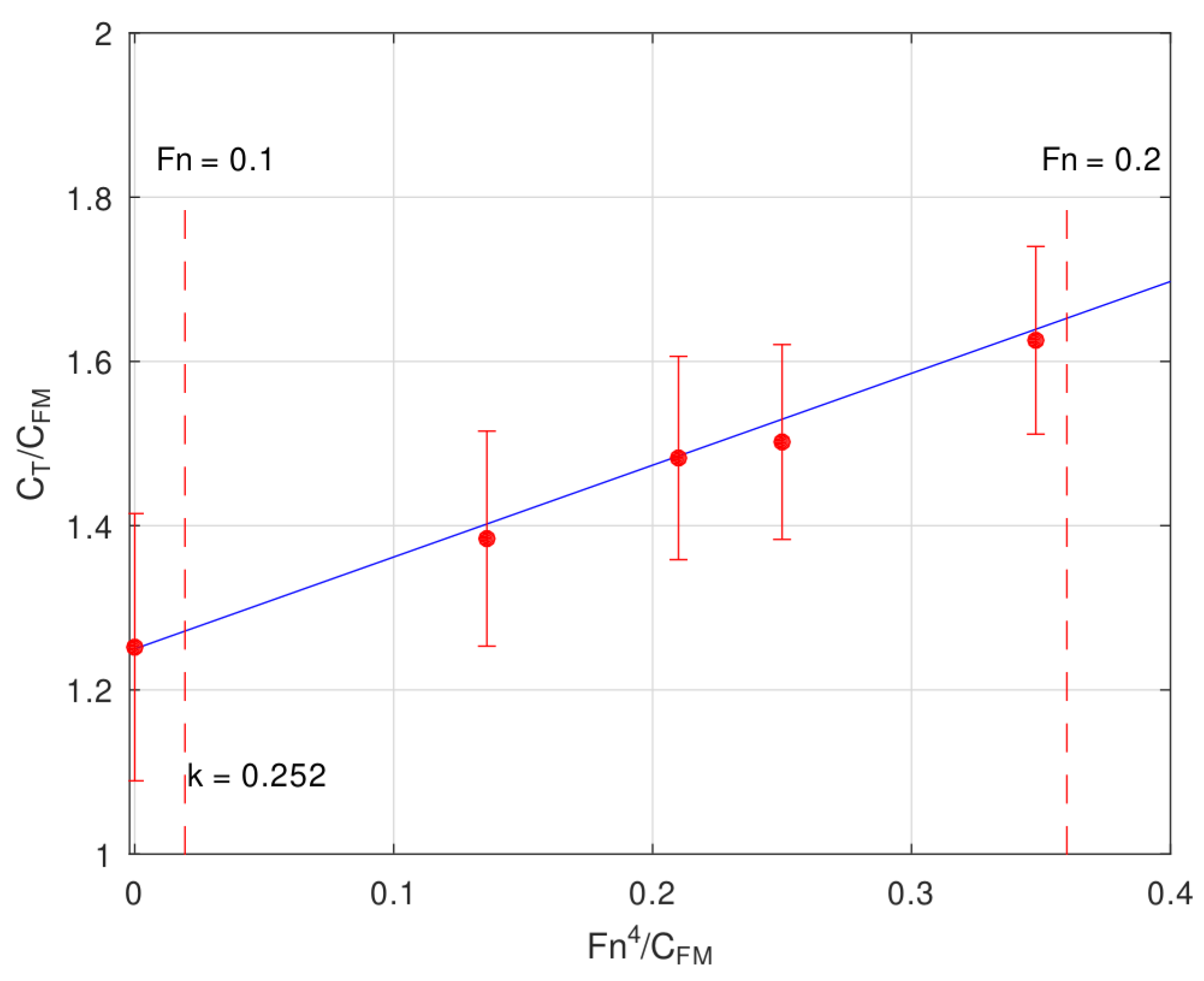
From the experimental results, we plot the left and right sides of Equation (8) as data points ($C_{TM}/C_{FM}$, Fn⁴/$C_{FM}$), where the data points should align in a straight line for model speeds with Fn < 0.2. The ITTC recommends using only data points in the Fn range [0.1, 0.2]. The form factor can then be determined by linear regression. In this paper, the regression lines were obtained by using the method explained by York [20].

As an example, Figure 9 shows the ($C_{TM}/C_{FM}$, Fn⁴/$C_{FM}$) points for T1 of 0.165 m (LC ballast) considering Fn < 0.2, along with the resulting regression line obtained by using York’s method. The dashed red vertical lines indicate the limits of the range of Fn as [0.1, 0.2]. This method accounts for the experimental uncertainties in the regression process and also predicts the uncertainties in the form factor, shown with an error bar at Fn⁴/$C_{FM}$ = 0. The uncertainty in the form factor was calculated to be 0.163, which is 65% of k for the 95% confidence interval. The error for each point, except for the extrapolation by York’s method at Fn = 0, was calculated as the “Expanded for repeat mean” presented in Table 2, given that the only source of error in $C_{TM}/C_{FM}$ is $C_{TM}$.

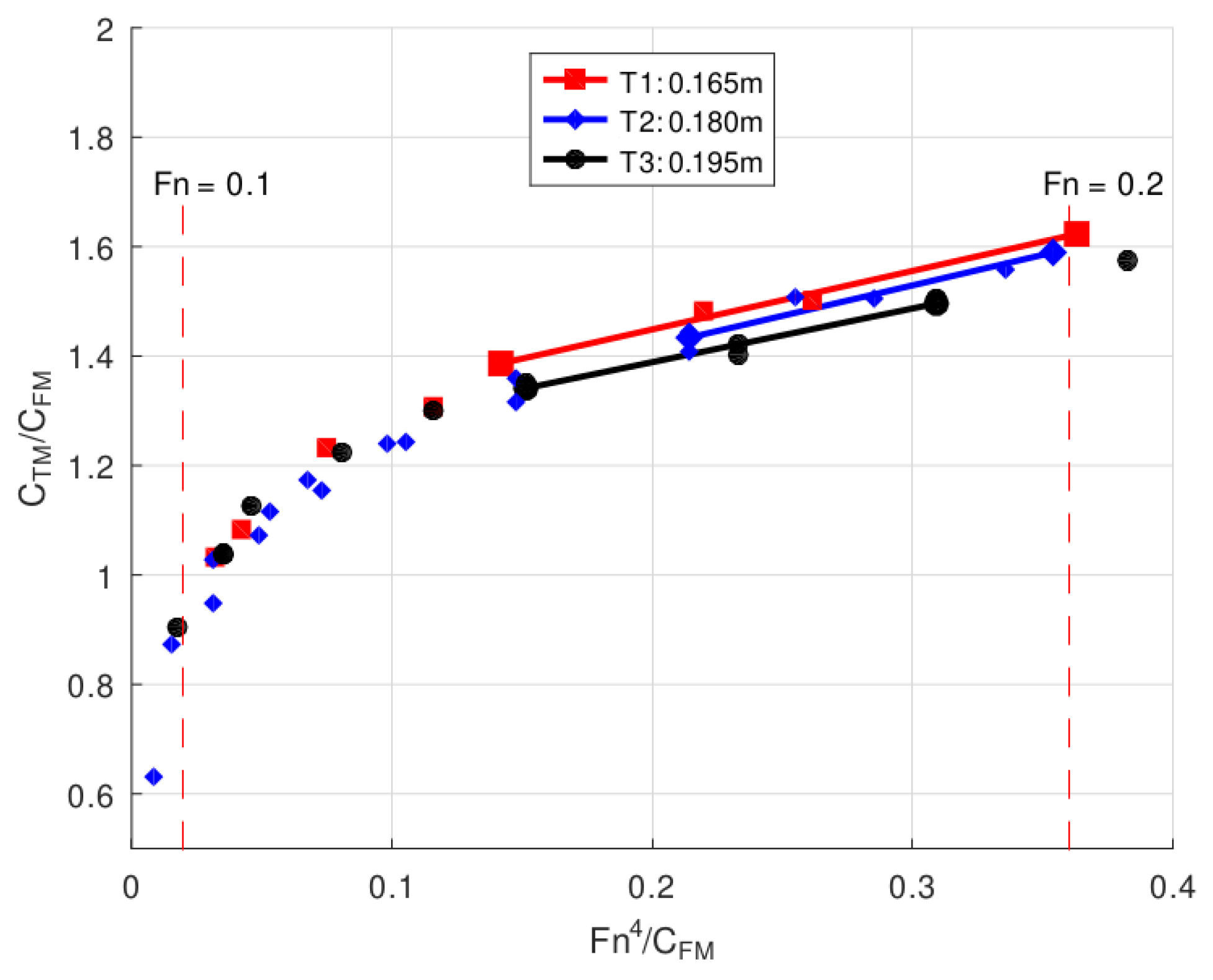
Equation (8), for 0.1 < Fn < 0.2, is plotted for the three different draughts in Figure 10.

It is worth noting that at very low values of Fn, the measured points deviate from a straight line, making it necessary to select an appropriate data set for each draught to determine the form factor. Figure 10 shows straight lines indicating the resulting slope to determine the form factor for each draught. These lines also delineate the Fn range considered in each case. Similarly to Figure 9, the dashed red vertical lines indicate the limits of the Fn range as [0.1, 0.2].

The form factors obtained for T1, T2 and T3, together with their uncertainties, are given in

Table 5. Form factors for different draughts calculated by Prohaska’s method.

Load Condition	k	${\mathit{U}}_{\mathit{k}}$%
T1: 0.165 m	0.252	65
T2: 0.180 m	0.211	77
T3: 0.195 m	0.194	90

.

It is crucial to highlight that despite being considered the most reliable procedure available, Prohaska’s method still yields results with high uncertainty. This elevated uncertainty in the value of k can be attributed to two primary factors. Firstly, the precise measurement of low-speed resistance at a model scale poses significant challenges, as elucidated in Section 2.3. Secondly, flow phenomena associated with very low model speeds play a role. Low model speed results in a low Reynolds number, increasing the likelihood of flow separation and hindering the transition of the boundary layer to turbulence. If separation occurs, it leads to increased resistance and consequently yields a larger form factor. Conversely, if the boundary flow remains predominantly laminar without separation, the form factors may become smaller. Moreover, the challenges related to low Reynolds numbers are exacerbated for shorter models (larger scales), such as the one examined in this study.

In addition, the ship analysed in this work has a bulbous bow and stern, which may affect the applicability of Prohaska’s method. These factors increase the uncertainties associated with low-speed drag measurements and low Reynolds number flow phenomena [21,22].

In Section 4.6, we consider the effect of the high uncertainty in the form factor on the extrapolation of drag to the full-scale ship.

4.4. Numerical Form Factor Determination

The calculation of the CFD form factor not only serves to decompose the total resistance (see Section 4.5) but also facilitates the investigation of the potential improvement in the extrapolation of the total vessel resistance by using combined CFD-EFD methods (see Section 4.6).

The CFD-based form-factor method considered for this study follows the assumptions of Hughes [19] and is derived using the relationship

$$(1+k)=\frac{C_F+C_{PV}}{C_{FM}}=\frac{C_V}{C_{FM}}$$

(9)

where the frictional drag coefficient ($C_F$) and the viscous pressure coefficient ($C_{PV}$) are obtained from the double-body CFD simulation. $C_{FM}$ in the denominator of Equation (9) represents the equivalent flat plate resistance obtained from the same Reynolds number as the calculations using the ITTC-57 friction line.

The uncertainty in the CFD form factor was calculated using the Grid Convergence Index (GCI) method described in [23].

Table 6. Form factors for different draughts, calculated by Prohaska’s method and double-hull CFD method.

CFD Double Hull	T1: 0.165 m		T2: 0.180 m		T3: 0.195 m
	$\mathit{k}$	${\mathit{U}}_{\mathit{k}}$ %	$\mathit{k}$	${\mathit{U}}_{\mathit{k}}$ %	$\mathit{k}$	${\mathit{U}}_{\mathit{k}}$ %
$\mathrm{Fn}=0.10$	0.168	13.32	0.157	0.12	0.179	4.08
$\mathrm{Fn}=0.20$	0.302	7.31	0.292	0.01	0.320	0.95

shows the CFD form factors for different draughts, obtained by the double-hull method (at Fn = 0.1 and Fn = 0.2), along with their associated numerical uncertainties.

It is important to note that the difference in CFD form factors for different Fn is much higher than the numerical uncertainty in k. This result seems to indicate a dependence of k on model velocity. In fact, the low Re number range (1.10⁶–3.10⁶) used in the model-scale experiments could produce some scale effects related to boundary-layer transition. The investigation of this dependence is outside the scope of this paper. We are currently working on verifying the occurrence of such a dependence and interpreting the physical mechanism involved in it, along the lines of the work in [5,24].

Table 7. Form factor for different draughts, calculated by Prohaska’s method and double-hull CFD method.

Method	T1: 0.165 m		T2: 0.180 m		T3: 0.195 m
	$\mathit{k}$	$\Delta \%$	$\mathit{k}$	$\Delta \%$	$\mathit{k}$	$\Delta \%$
EFD Prohaska	0.252	0	0.211	0	0.194	0
CFD double hull Fn = 0.10	0.168	−33	0.157	−26	0.179	−8
CFD double hull Fn = 0.20	0.302	20	0.292	38	0.320	65

compares the CFD form factors, for the different draughts, obtained by the double-hull method (with Fn = 0.1 and Fn = 0.2) with the EFD obtained by Prohaska’s method (see Section 4.3). Table 7 shows the percentage difference between the EFD and CFD form factors, taking the EFD form factor as the reference value. In all cases, the difference between the CFD and EFD form factors is significant. However, it is still smaller than the uncertainty in the experimental form factor.

4.5. Viscous and Wave Drag Components

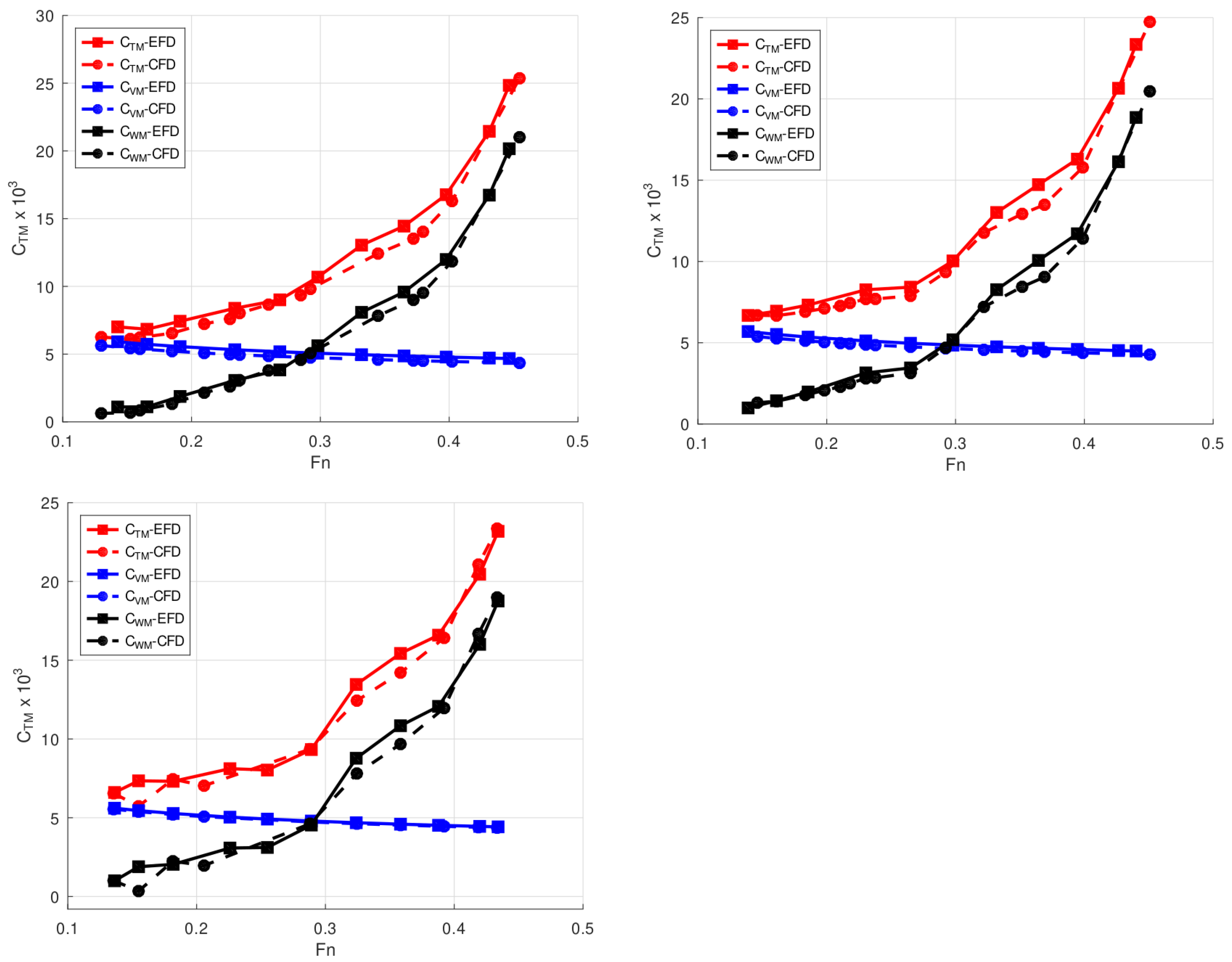
To provide a better understanding of how the viscous and wave components contribute to total drag, the total drag coefficient was split into viscous and wave coefficients by using the obtained form factor.

Figure 11 illustrates the numerically and experimentally obtained curves of $C_{TM}$, $C_{VM}=(1+k)C_{FM}$ and $C_W$ (calculated as $C_{TM}-C_{VM}$) versus Fn for different draughts. The form factor (k) used in the EFD curves is the one derived from the experimental data (see Section 4.3), while the k used in the CFD curves is the one obtained numerically with Fn = 0.1 (see Section 4.4). In both cases, $C_{FM}$ corresponds to the ITTC-57 friction line.

Figure 11 demonstrates the ability of the CFD model to decompose the total resistance of the model into wave and viscous resistance components by using the double-body approach to obtain the form factor. A general good agreement between the EFD and CFD results is observed for the three draughts studied and the different Froude numbers. From Figure 11, it can be seen that for Fn < 0.2, the viscous resistance is significantly larger compared with the wave resistance component. However, for Fn > 0.3, the wave component, which initially has a similar value to the viscous resistance, increases proportionally to Fn⁴ and quickly becomes the most significant resistance component. For example, at Fn = 0.30, Fn = 0.37 and Fn = 0.40, the wave resistance represents approximately 47%, 63% and 70% of the total resistance, respectively. Finally, for Fn > 0.4, the $C_W$ curves tend to converge towards the $C_{TM}$ curves, indicating that the wave resistance is more than 80% of the total resistance.

4.6. Comments on the Combined EFD-CFD Approach

The results of the towing tank tests could be extrapolated to estimate the resistance values of the full-scale ship by using the ITTC performance prediction method [25]. This method assumes that the wave resistance coefficient ($C_W$) of the ship is independent of scale effects and that the ratio of the viscous pressure resistance coefficient to the frictional resistance coefficient is constant, so that the form factor is constant. The extrapolation formula for the method is as follows:

$$C_{TS}=C_{TM}+(1+k)(C_{FS}-C_{FM})+\Delta C_F+C_A$$

(10)

where $C_{TS}$ and $C_{TM}$ are the total ship and model drag coefficients, respectively, and $C_{FS}$ and $C_{FM}$ are the frictional ship and model drag coefficients, respectively. The coefficient of friction ($C_F$) is calculated by using the ITTC 1957 correlation line.

A roughness allowance ($\Delta C_F$) is applied to account for the relative increase in frictional resistance from model-scale to full-scale vessels, and a correlation allowance ($C_A$) is applied to account for remaining differences between model-scale and full-scale vessels. Both $\Delta C_F$ and $C_A$ were calculated according to [25]. The $\Delta C_F$ allowance depends on the full scale equivalent sand roughness (we adopted the standard value of 150 $\mathsf{\mu }$m), waterline length ($L_{WL}$) and Reynolds number ($Re$). The $C_A$ allowance depends only on the full-scale Reynolds number ($Re$).

Equation (10) clearly shows the importance of the correct determination of the form factor in predicting the total resistance for the full-scale ship. If the form factor is set too high, the resistance of the full-scale ship will be under predicted because the wave resistance estimate will be too low, and vice versa. The uncertainty in the value of k does not directly translate into the uncertainty in the value of $C_{TS}$, as it does not affect all terms of the equation equally.

Table 8. $\Delta C_{TS}$. Error in estimating $C_{TS}$ taking into account the uncertainty in the value of k.

Method	${\mathit{V}}_{\mathit{S}}$ (kn)	Fn	$\Delta$${\mathit{C}}_{\mathit{TS}}$ %
			T1	T2	T3
EFD CTM from EFD (k and Uk from Table 5)	5.5	0.16	−8.77	−8.23	−8.11
	8.0	0.23	−5.68	−5.60	−6.09
	10.5	0.30	−3.85	−4.01	−4.68
CFD-EFD CTM from EFD (k and Uk from Table 6)	5.5	0.16	−1.15	0.01	−0.34
	8.0	0.23	−0.75	0.01	−0.25
	10.5	0.30	−0.52	0.01	−0.19
CFD-CFD CTM from CFD (k and Uk from Table 6)	5.5	0.16	−1.01	0.01	−0.44
	8.0	0.23	−0.88	0.01	−0.31
	10.5	0.30	−0.50	0.01	−0.20

displays the error in estimating $C_{TS}$ for three different approaches or methods, taking into account the uncertainty in the value of k. The first approach is the classical EFD approach, which considers the EFD k and $U_k$ values in Table 5, as well as the EFD $C_{TM}$ values. The second approach is the combined CFD-EFD method, which considers the CFD k and $U_k$ values in Table 6 for Fn = 0.1, along with the EFD $C_{TM}$ values. The third and final approach is a pure CFD approach, which takes into account the CFD k and $U_k$ values in Table 6 for Fn = 0.1, as well as the CFD $C_{TM}$ values.

Table 8 shows that Prohaska’s method’s experimental determination of k for this type of ship results in high uncertainty values, leading to a significant uncertainty in $C_{TS}$. However, when k is numerically determined, the CFD-EFD and CFD methods result in significantly lower uncertainty values for $C_{TS}$.

5. Conclusions

In this study, both numerical and experimental methods were used to determine the total ship resistance for a fishing vessel model. The results from both approaches showed good agreement over a range of speeds and loading conditions, with discrepancies of less than 8% between them.

The numerical analysis showed that the wave distribution around the model hull closely matched the observations from the experimental towing tank tests. This successful validation of the CFD model indicates its suitability for hydrodynamic studies of the fishing vessel model.

In addition, the pressure distribution on the hull obtained by the CFD model provided crucial insights into the phenomenon of wave resistance, which is essential to evaluating the vessel’s performance. Understanding the relationship between the wave pattern and the pressure distribution on the hull is crucial to designing and operating efficient vessels.

Form factors were determined both numerically and experimentally, allowing for a comparison of the different resistance components based on Hughes’ hypothesis. Strong agreement was found between the EFD and CFD viscous and wave resistance coefficients for different draughts and Froude numbers.

In particular, the CFD double-body model allowed a form factor to be obtained with significantly less uncertainty compared with experimental methods. This suggests that CFD-based form factors could serve as a viable alternative to Prohaska’s method, potentially improving ship performance prediction through combined CFD-EFD methods.

Future research directions could include further investigation of wave resistance and ship hydrodynamic optimisation for this type of fishing vessel.

In addition, the investigation of the dependence of the form factor on factors such as model speed, scale effects and the presence of bulbous bows and transoms would be valuable in refining power prediction methods using combined CFD-EFD approaches.

References

- Holtrop, J. A statistical re-analysis of resistance and propulsion data. Int. Shipbuild. Prog. 1984, 31, 272–276. [Google Scholar]
- Bilec, M.; Obreja, C.D. Ship resistance and powering prediction of a fishing vessel. IOP Conf. Ser. Mater. Sci. Eng. 2020, 916, 012011. [Google Scholar] [CrossRef]
- Larsson, L.; Stern, F.; Visonneau, M. (Eds.) Numerical Ship Hydrodynamics: An Assessment of the Gothenburg 2010 Workshop; Springer: Dordrecht, The Netherlands, 2013. [Google Scholar]
- Hino, T.; Stern, F.; Larsson, L.; Visonneau, M.; Hirata, N.; Kim, J. (Eds.) Numerical Ship Hydrodynamics: An Assessment of the Tokyo 2015 Workshop; Springer: Cham, Switzerland, 2021. [Google Scholar] [CrossRef]
- Terziev, M.; Tezdogan, T.; Incecik, A. Scale effects and full-scale ship hydrodynamics: A review. Ocean. Eng. 2022, 245, 110496. [Google Scholar] [CrossRef]
- 29th ITTC Resistance Committee. ITTC—The Specialist Committee on CFD and EFD Combined Methods Final Report and Recommendations; ITTC. 2021. Available online: https://ittc.info/media/10940/volume-ii.pdf (accessed on 4 March 2024).
- Prohaska, C. A simple method for evaluation of the form facter and low speed wave resistance. In Proceedings of the 11th ITTC, Tokyo, Japan, 11–20 October 1966; pp. 65–66. [Google Scholar]
- Garcia-Gómez, A. On the form factor scale effect. Ocean. Eng. 2000, 27, 97–109. [Google Scholar] [CrossRef]
- Terziev, M.; Tezdogan, T.; Incecik, A. A geosim analysis of ship resistance decomposition and scale effects with the aid of CFD. Appl. Ocean. Res. 2019, 92, 101930. [Google Scholar] [CrossRef]
- Dogrul, A.; Song, S.; Demirel, Y.K. Scale effect on ship resistance components and form factor. Ocean. Eng. 2020, 209, 107428. [Google Scholar] [CrossRef]
- Korkmaz, K.B.; Werner, S.; Bensow, R.E. Numerical Friction Lines for CFD Based Form Factor Determination Method. In Proceedings of the VIII International Conference on Computational Methods in Marine Engineering, Gothenburg, Sweden, 13–15 May 2019. [Google Scholar]
- Korkmaz, K.B.; Werner, S.; Sakamoto, N.; Queutey, P.; Deng, G.; Yuling, G.; Guoxiang, D.; Maki, K.; Ye, H.; Akinturk, A.; et al. CFD based form factor determination method. Ocean. Eng. 2021, 220, 108451. [Google Scholar] [CrossRef]
- Bertolotti, M.; Verazay, G.; Pagani, A.; Errazti, E.; Buono, J. Flota pesquera Argentina. Evolucion 1960–1998 con una actualizacion al 2000. In El Mar Argentino y sus Recursos Pesqueros; Ministerio de Agroindustria: Mar del Plata, Argentina, 2001. [Google Scholar]
- Specialist Committee: Procedures for Ship Models; of 28th ITTC 2017 ITTC—Recommended Procedures and Guidelines: Model Manufacture, Ship Models; ITTC, 2017. Available online: https://www.ittc.info/media/7975/75-01-01-01.pdf (accessed on 4 March 2024).
- 26th ITTC Resistance Committee. ITTC—Recommended Procedures and Guidelines—Resistance Test; ITTC, 2011. Available online: https://ittc.info/media/1217/75-02-02-01.pdf (accessed on 4 March 2024).
- 28th ITTC Quality Systems Group. ITTC—General Guidelines for Uncertainty Analisys in Resistance Tests; ITTC, 2021. Available online: https://www.ittc.info/media/9601/75-02-02-02.pdf (accessed on 4 March 2024).
- Díaz-Ojeda, H.; Pérez-Arribas, F.; Turnock, S.R. The influence of dihedral bulbous bows on the resistance of small fishing vessels: A numerical study. Ocean. Eng. 2023, 281, 114661. [Google Scholar] [CrossRef]
- Blount, D. Performance by Design: Hydrodynamics for High-Speed Vessels; Donald L. Blount: Chesapeake, VA, USA, 2014. [Google Scholar]
- Hughes, G. Friction and Form Resistance in Turbulent Flow, and a Proposed Formulation for Use in Model and Ship Correlation. National Physical Laboratory, NPL, Ship Division, Presented at the Institution of Naval Architects, Paper No. 7, London, April, RINA Transactions 1954-16. 1954. Available online: http://resolver.tudelft.nl/uuid:9a642c53-27f0-45fe-a5e4-5e1296b62af1 (accessed on 4 March 2024).
- York, D.; Evensen, N.; Ló, M.; Nez, M.; De, J.; Delgado, B. Unified equations for the slope, intercept, and standard errors of the best straight line. Am. J. Phys. 2004, 72, 367–375. [Google Scholar] [CrossRef]
- 14th ITTC Performance Committee. Form factor. In Proceedings of the 14th ITTC, Ottawa, ON, Canada, 2–11 September 1975. [Google Scholar]
- Korkmaz, K.B.; Werner, S.; Bensow, R. Scaling of wetted-transom resistance for improved full-scale ship performance predictions. Ocean. Eng. 2022, 266, 112590. [Google Scholar] [CrossRef]
- 28th ITTC Resistance Comittee. Uncertainty Analysis in cfd Verification and Validation, Methodology and Procedures. ITTC—Quality System Manual Recommended Procedures and Guidelines 7, 5-03-01-01; ITTC: 2017. Available online: https://www.ittc.info/media/8153/75-03-01-01.pdf (accessed on 4 March 2024).
- Terziev, M.; Tezdogan, T.; Demirel, Y.K.; Villa, D.; Mizzi, S.; Incecik, A. Exploring the effects of speed and scale on a ship’s form factor using CFD. Int. J. Nav. Archit. Ocean. Eng. 2021, 13, 147–162. [Google Scholar] [CrossRef]
- 28th ITTC Propulsion Committee. ITTC—Recommended Procedures and Guidelines—1978 ITTC Performance Prediction Method; ITTC, 2017. Available online: https://www.ittc.info/media/8017/75-02-03-014.pdf (accessed on 4 March 2024).
Figure 1.
Body lines of the case study ship.
Figure 2.
Problem setup and main parameters.
Figure 3.
General mesh view. Mesh 4.
Figure 4.
Mesh zoom for different orientations. Mesh 4.
Figure 5.
vs. Fn for different draughts. Top left: T1 (0.165 m). Top right: T2 (0.180 m). Bottom: T3 (0.195 m).
Figure 6.
vs. Fn. Left: all draughts on EFD; right: all draughts on CFD.
Figure 7.
Wave pattern for different Fn and draught = T3. Left column: 3D CFD model. Right column: EFD model. First row: Fn = 0.26; second row: Fn = 0.37; third row: Fn = 0.45.
Figure 8.
distribution for different Fn at T3. First row: Fn = 0.26; second row: Fn = 0.37; third row: Fn = 0.45.
Figure 9.
Experimental form factor determination by Prohaska’s method with a regression line obtained by York’s method (T1: 0.165 m).
Figure 10.
Experimental form factor determination by using Prohaska’s method applied to the three different designs.
Figure 11.
, and vs. Fn. for different draughts. Top left: T1 (0.165 m). Top right: T2 (0.180 m). Bottom: T3 (0.195 m).