An Improved Identification Method of Pipeline Leak Using Acoustic Emission Signal

Abstract

Pipelines constitute a vital component in offshore oil and gas operations, subjected to prolonged exposure to a range of alternating loads. Safeguarding their integrity, particularly through meticulous leak detection, is essential for ensuring safe and reliable operation. Acoustic emission detection emerges as an effective approach for monitoring pipeline leaks, demanding subsequent rigorous data analysis. Traditional analysis techniques like wavelet analysis, empirical mode decomposition (EMD), variational mode decomposition (VMD), and complete ensemble empirical mode decomposition with adaptive noise (CEEMDAN) often yield results with considerable randomness, adversely affecting leak detection accuracy. This study introduces an enhanced damage recognition methodology, integrating improved complete ensemble empirical mode decomposition with adaptive noise (ICEEMDAN) and probabilistic neural networks (PNN) for more accurate pipeline leak identification. This novel approach combines laboratory-acquired acoustic emission signals from leaks with ambient noise signals. Application of ICEEMDAN to these composite signals isolates eight intrinsic mode functions (IMFs), with subsequent time–frequency analysis providing insight into their frequency structures and feature vectors. These vectors are then employed to train a PNN, culminating in a robust neural network model tailored for leak detection. Conduct experimental research on pipeline leakage identification, focusing on the local structure of offshore platforms, experimental research validates the superiority of the ICEEMDAN–PNN model over existing methods like EMD, VMD, and CEEMDAN paired with PNN, particularly in terms of stability, anti-interference capabilities, and detection precision. Notably, even amidst integrated noise, the ICEEMDAN–PNN model maintains a remarkable 98% accuracy rate in identifying pipeline leaks.

1. Introduction

Natural gas plays a crucial role in people’s production and daily lives, accounting for 24% of the global total energy consumption [1]. As a critical infrastructure for the extraction and transportation of oil and gas, pipeline systems offer significant advantages such as high capacity and low cost, playing an essential role in various processes of offshore oil and gas exploration, production, and transportation. However, due to the harsh working conditions in offshore environments, pipeline systems are subjected to long-term effects of various cyclic loads. Under the combined action of corrosion, wear, sudden natural disasters, and internal pressure differentials, they are more prone to fatigue damage, leading to leaks in the pipeline. This can have destructive impacts on the human environment, production, life, and property safety [2,3]. Therefore, leakage detection for pipeline systems holds significant practical significance in promoting national economic development.

Various scholars in the relevant field have proposed multiple methods for leakage detection in pipeline systems, including visual inspection, negative pressure wave method, eddy current detection, fiber optic grating method, and acoustic methods, among others [4,5,6,7,8,9,10]. Among these, acoustic emission technology, as a novel non-destructive testing technique, has the unparalleled advantages of dynamically, sensitively, and comprehensively recording the irreversible changes in composite materials through elastic waves. It reflects the damage situation of materials and structures with high sensitivity, real-time prediction, and long-distance detection, which are incomparable to other detection methods [11,12]. Numerous acoustic emission characteristic parameters, including energy, duration, impact count, amplitude, signal strength, peak frequency, rise time, etc., can be extracted from acoustic emission signals [13,14,15,16,17]. To investigate the damage situation of structures, these characteristic parameters can be used individually or in combination [18]. When certain acoustic emission characteristic parameters are combined, damage pattern recognition can be achieved, thereby identifying the acoustic emission features of specific damage patterns [19,20,21,22]. Therefore, the application of acoustic emission technology in the field of structural health monitoring (SHM) is gaining increasing attention [23].

The precise characterization of structural damage states through the application of acoustic emission non-destructive monitoring technology has become a focal point for researchers, and a substantial amount of experimental research has been conducted by relevant scholars. In the 1950s, the German researcher Kaiser [24] first discovered the phenomenon of acoustic emission in metal deformation and proposed the concepts of burst-type and continuous-type acoustic emission signals. Over more than half a century of development, both the technology and theory of acoustic emission have significantly improved and found extensive applications in various industries, such as civil engineering, petrochemicals, aerospace, and marine engineering [25,26,27,28,29,30,31], indicating a promising future. Meniconi, S et al. [32,33] innovatively proposed a transient analysis method for fault diagnosis of underwater pipelines, which holds significant implications for the advancement of SHM techniques. Grabec I [34] simulated burst-type and continuous-type acoustic emission signals through experiments on aluminum strips and suggested that time delay estimation using the correlation method is feasible, laying the groundwork for subsequent applications of acoustic emission in pipeline leak detection. Pollock A A et al. [35], through pipeline leak experiments, collected abundant waveform information about continuous leak acoustic emission signals. Clark M A et al. [36,37] investigated the issue of acoustic signal attenuation in fully liquid-filled pipelines and found that the type of backfill material used for pipelines filled with fluid significantly affects signal attenuation. In the same year, the team proposed utilizing the frequency dispersion characteristics of waves in pipelines for leak source localization, establishing a dispersion model for liquid-filled pipelines. Miller R K et al. [38] established equipment-related settings and evaluation reference standards for acoustic emission devices used in pipeline leak detection. They pointed out that minor leakage phenomena in actual pipelines are often related to flange gaskets and threads. Jiao J et al. [39], through experiments, verified the multimodal propagation and dispersion characteristics of sound waves in pipelines, proposing a single-sensor modal acoustic emission (MAE) pipeline leak localization technology. Ozevin D et al. [40], by arranging an array of acoustic emission sensors on the surface of a PVC pipeline network, used a one-dimensional acoustic emission source localization algorithm to determine the two-dimensional location of pipeline leaks. By combining the relationship between attenuation and wave velocity with the localization algorithm, they significantly enhanced the reliability of leak localization.

In recent years, there has been significant progress in acoustic emission-based pipeline leakage detection technology. To promote the extension and application of acoustic emission technology in the field of structural health monitoring, scholars have conducted acoustic emission experiments to collect acoustic emission signals. Subsequently, they further analyzed and processed the collected acoustic emission signals. In the analysis process, wavelet theory [41,42] is often used as a time–frequency processing method to handle acoustic emission signals. The signals obtained after decomposition using this method contain relevant information about the working condition and faults of specific mechanical components. Therefore, based on this decomposed information, it becomes more convenient and efficient to monitor and diagnose the damage state of structures. In structural health monitoring, when the collected raw signals consist of short-term high-frequency components combined with long-term low-frequency components, the wavelet transform (WT) method exhibits excellent performance. However, the Mallat algorithm in wavelet transform cannot decompose high-frequency sequences, leading to the development of wavelet packet decomposition (WPT) [43], addressing the shortcomings of wavelet transform. Nevertheless, both WT and WPT require the pre-determination of wavelet basis functions and decomposition levels, lacking reliable performance metrics to evaluate the effectiveness of decomposition. In contrast, time–frequency processing methods based on empirical mode decomposition (EMD) and Hilbert–Huang transform (HHT) can adaptively decompose signals into independent components, overcoming the limitations of wavelet transform. Huang [44] first proposed the EMD method, which automatically decomposes signals into a set of intrinsic mode functions (IMF). This method has been widely applied in mechanical fault diagnosis. However, in practical applications, the EMD algorithm exhibits mode mixing and endpoint effects, restricting its use. To address this issue, Wu [45] introduced ensemble empirical mode decomposition (EEMD), which adds Gaussian white noise to EMD and then averages it several times to offset the noise. Although this method somewhat reduces the problem of mode mixing, it has lower decomposition efficiency and still exhibits mode mixing and energy leakage issues in the low-frequency region. Building on this, Torres [46] proposed complete EEMD with adaptive noise (CEEMDAN), which effectively handles nonlinear and non-stationary signals. Due to its adaptive addition of Gaussian white noise at each stage of the decomposition process, CEEMDAN achieves very low reconstruction errors and produces better modal frequency spectrum separation results. Its decomposition performance surpasses EMD and EEMD. However, the CEEMDAN algorithm lacks effective theoretical guidance for choosing the intensity of added white noise and the number of ensembles. Derived from the EMD algorithm, Smith [47] introduced local mean decomposition (LMD), which replaces cubic spline interpolation in EMD with a moving average. Similar to the EMD algorithm, the LMD algorithm adaptively decomposes complex multi-component amplitude and frequency-modulated signals into multiple product functions and a residue using extremum information. LMD outperforms EMD in suppressing endpoint effects and preserving signal information but still suffers from mode mixing problems. Dragomiretskiy [48,49,50] and others proposed variational mode decomposition (VMD). In the VMD algorithm, it is assumed that the Fourier spectrum of the signal has compact support. It constructs a set of Wiener filters to simultaneously extract all modes, and each mode is also mostly compact near its center frequency. VMD has found wide application in mechanical fault diagnosis. However, compared to EMD, which is independent of prior knowledge, the performance of the VMD algorithm is influenced by pre-defined mode numbers and penalty parameters. As each time–frequency processing algorithm has its own strengths and limitations, the appropriate time–frequency processing method should be chosen for different signals and applications.

In recent years, significant progress has been made in acoustic emission-based pipeline leakage detection technology. For offshore platform oil and gas pipeline systems, the extreme and harsh working environment poses challenges to the effectiveness of pipeline leakage detection using acoustic emission sensors, due to their high sensitivity. External interferences can easily affect the accuracy of leak detection. Traditional methods perform poorly when dealing with signals containing substantial noise interference, making it challenging to effectively identify acoustic emission signals associated with pipeline leaks. This results in time-consuming, costly, and less accurate processes. Therefore, effectively addressing these challenges has become a crucial technical issue for the practical application of acoustic emission technology in production.

This study proposes a damage identification method that combines acoustic emission technology with an improved modal decomposition algorithm. Using algorithms such as EMD, VMD, CEEMDAN, and ICEEMDAN, along with the PNN probability neural network, the features of leakage signals and noise signals are thoroughly analyzed and studied. Through this approach, the research achieves the goal of accurately identifying pipeline leak information, even in high-noise interference environments.

2. Pipeline Leak Experiments and Signal Feature Analysis

To simulate the realistic operating conditions of offshore oil and gas pipeline systems, this study conducted comprehensive pipeline leak experiments. The experiments were divided into two main parts: first, laboratory-based simulated pipeline leak experiments aimed to replicate pipeline leaks under different conditions, collecting corresponding acoustic emission signals; second, on-site noise experiments conducted on pressure pipelines on offshore platforms focused on collecting real-time noise data. Subsequently, we performed integrated processing on these collected signals to more accurately simulate acoustic emission signals from pipeline leaks in actual operational environments. Through a comparative analysis of integrated acoustic emission signals in both the time and frequency domains, the target is to reveal the unique characteristics of the acoustic emission signals associated with pipeline leaks.

2.1. Laboratory Pipeline Leak Experiment

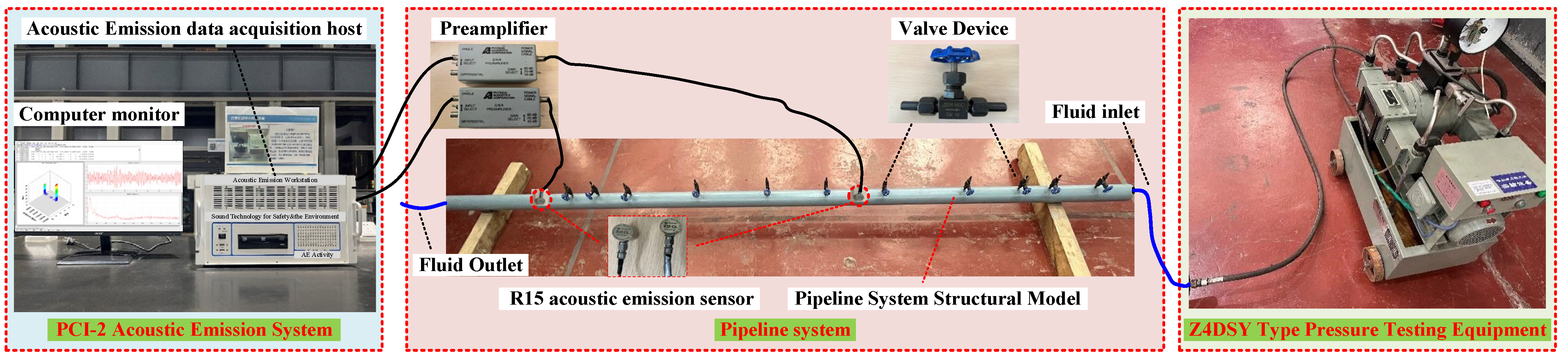
This experiment utilized a PCI-2 type acoustic emission device with a sampling frequency ranging from 1 kHz to 3 MHz. The equipment includes an R15 type acoustic emission sensor with a central frequency of 150 kHz and a pre-amplifier with amplification factors of 20/40/60 dB.

The pipeline leak experiment system consists of a pressure pipeline, pump, pressure gauge, control valves, and other components, enabling experimental analysis under different pressures, leak apertures, and leak positions. The schematic diagram of the experimental setup is shown in Figure 1.

The pipeline model used conforms to the specifications outlined in GB/T 8163-2018 for seamless steel pipes used in conveying high-pressure fluids. This material is commonly employed for constructing pipelines on offshore platforms [51]. The pipeline has a diameter of 105 mm, a wall thickness of 5 mm, and a total length of 6.2 m. The structure of the pipeline system primarily consists of two parts: a 5 m experimental section with 11 high-pressure welded needle valves distributed within it, simulating various leakage scenarios. The other part is a 1.2 m buffer zone, connected to the pressurization device via rubber pipelines. Different pipeline internal pressure conditions are achieved through the Z4DSY-type pressure application device.

Utilizing the aforementioned experimental system, pipeline leak experiments were conducted to investigate the propagation characteristics of leakage acoustic emission signals. Simulated pipeline leak experiments were carried out under different pressures and sensor spacings, studying the varying characteristics of pipeline leak acoustic emission signals under different conditions.

Two R15-type acoustic emission sensors were positioned at a distance of 10 cm from the ends of the pipeline, adjacent to the boundaries of the experimental section. Industrial-grade petroleum jelly was employed as a coupling agent between the pipeline surface and the acoustic emission sensors. The sensors were secured using tape. The downstream sensor was designated as Sensor 1, and the distances of each valve relative to Sensor 1 are presented in

Table 1. Positions of Each Valve (mm).

Identification Code	1	2	3	4	5	6	7	8	9	10	11
Location	207	567	807	1253	1923	2406	2895	3500	4105	4397	4640

.

The coupling condition between the acoustic emission sensors and the pipeline surface was assessed through a lead break test. Subsequently, laboratory noise was collected by closing the valves to maintain a balanced flow in the inlet and outlet pipelines, capturing noise information in the absence of any leaks. Pipeline leak experiments were then conducted at pressures of 1.0 MPa, 2.0 MPa, and 3.0 MPa. Multiple sets of leakage acoustic emission signal data were collected under different positions and pressure distributions.

2.2. Offshore Platform Field Noise Experiment

Acoustic emission technology can detect the initiation and evolution of early-stage cracks in pipelines. Due to the relatively complex nature of on-site working environments and considering that the collected acoustic emission data is often subject to various environmental noises, it significantly impacts the extraction of acoustic emission characteristic signals. Therefore, it is necessary to collect on-site environmental noise signals for the analysis and processing of experimental results.

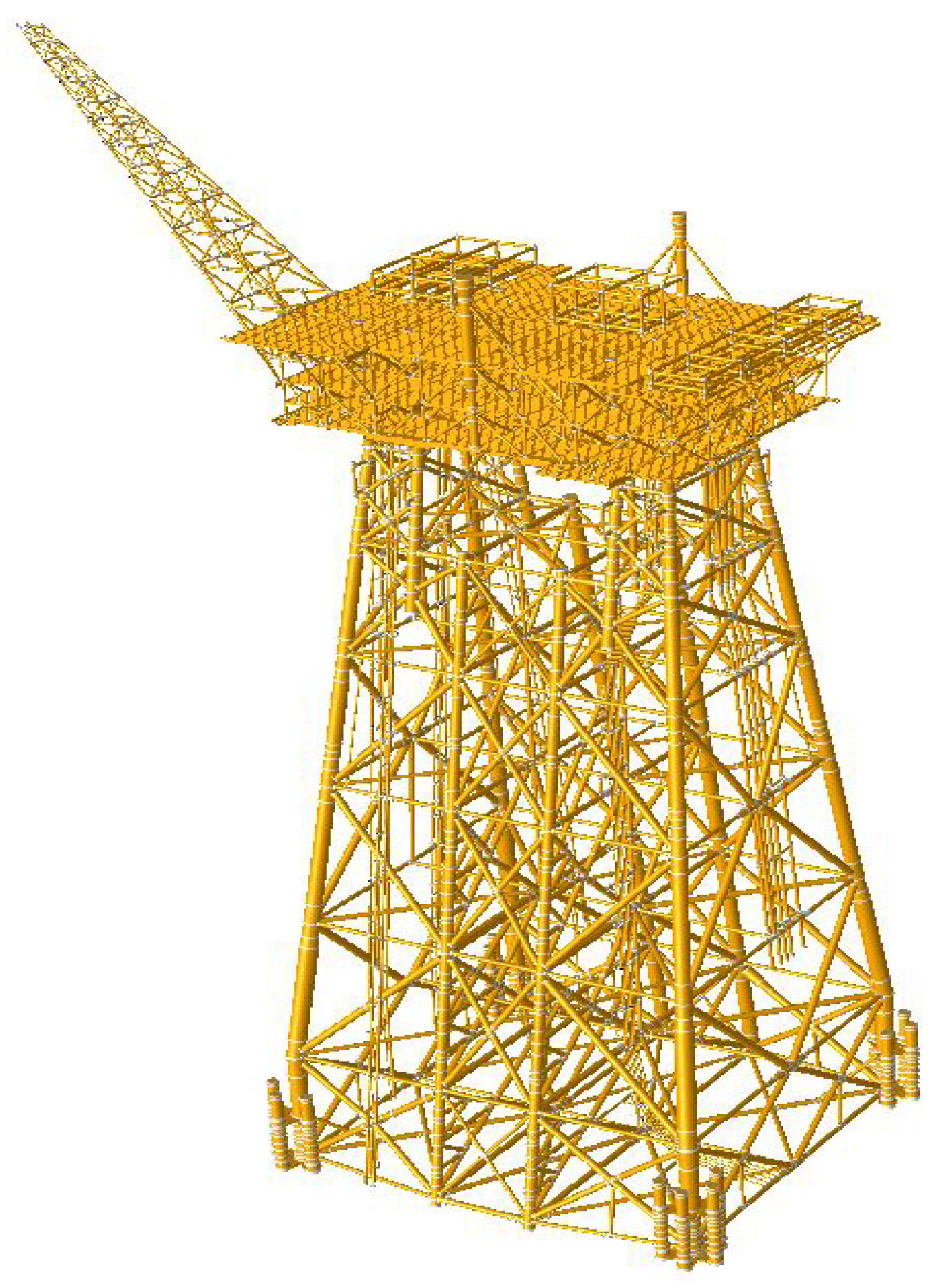
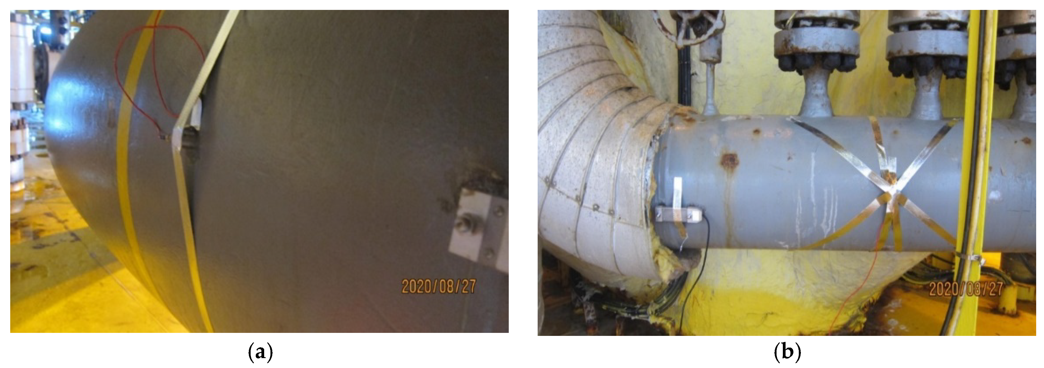
The on-site noise experiment was conducted at an offshore testing platform located in the Pearl River Mouth Basin, China (19°54′42.93″ N, 115°24′07.17″ E, with a block area of approximately 3965 km²). The platform, adopting an 8-legged template structure connected to the seabed by 16 skirt piles, is situated at a water depth of 191 m, as depicted in Figure 2. On this platform, field noise signals were experimentally collected from the pipeline to investigate the impact of on-site noise on the detection of acoustic emission signals related to pipeline leaks.

Based on on-site research analysis and considering the actual operating conditions of the platform, it was identified that the 19-m platform location experiences significant pipeline vibrations, exhibiting typical mechanical vibration noise and a proneness to fatigue damage. At the 29-m platform location, there is a typical elbow pipeline that undergoes cooling treatment after compression by a compressor, experiencing high pressure and stress concentration at the elbow, leading to structural fatigue damage. Therefore, the 19-m and 29-m platform positions were selected as typical test points for measurement, as shown in Figure 3. At the aforementioned typical locations, acoustic emission sensors were strategically placed, and the collection equipment, along with basic parameter settings, remained consistent with laboratory conditions. Subsequently, long-term scheduled sampling was conducted to collect on-site environmental noise signals.

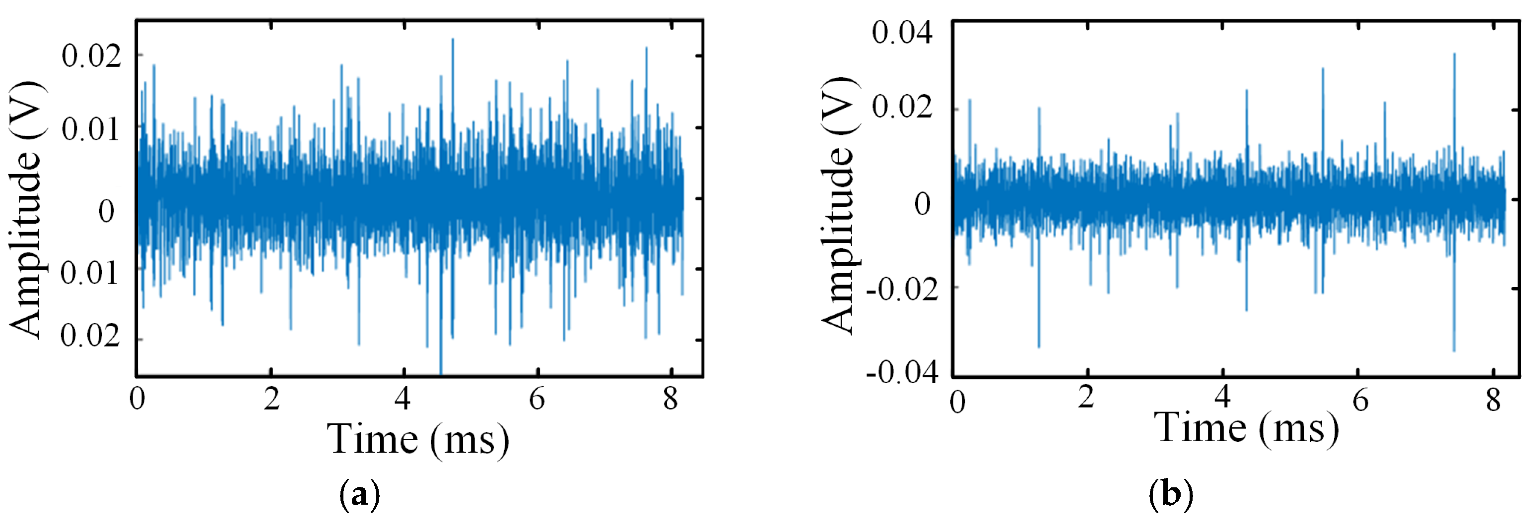
Through the collection and analysis of on-site noise signals, the temporal waveform was obtained, as illustrated in Figure 4.

It can be observed that the platform noise signals in the time domain also exhibit continuous acoustic emission characteristics. Although there are some abnormal peak signals in the waveform, the overall amplitude is in the same order of magnitude as the leakage signal amplitude.

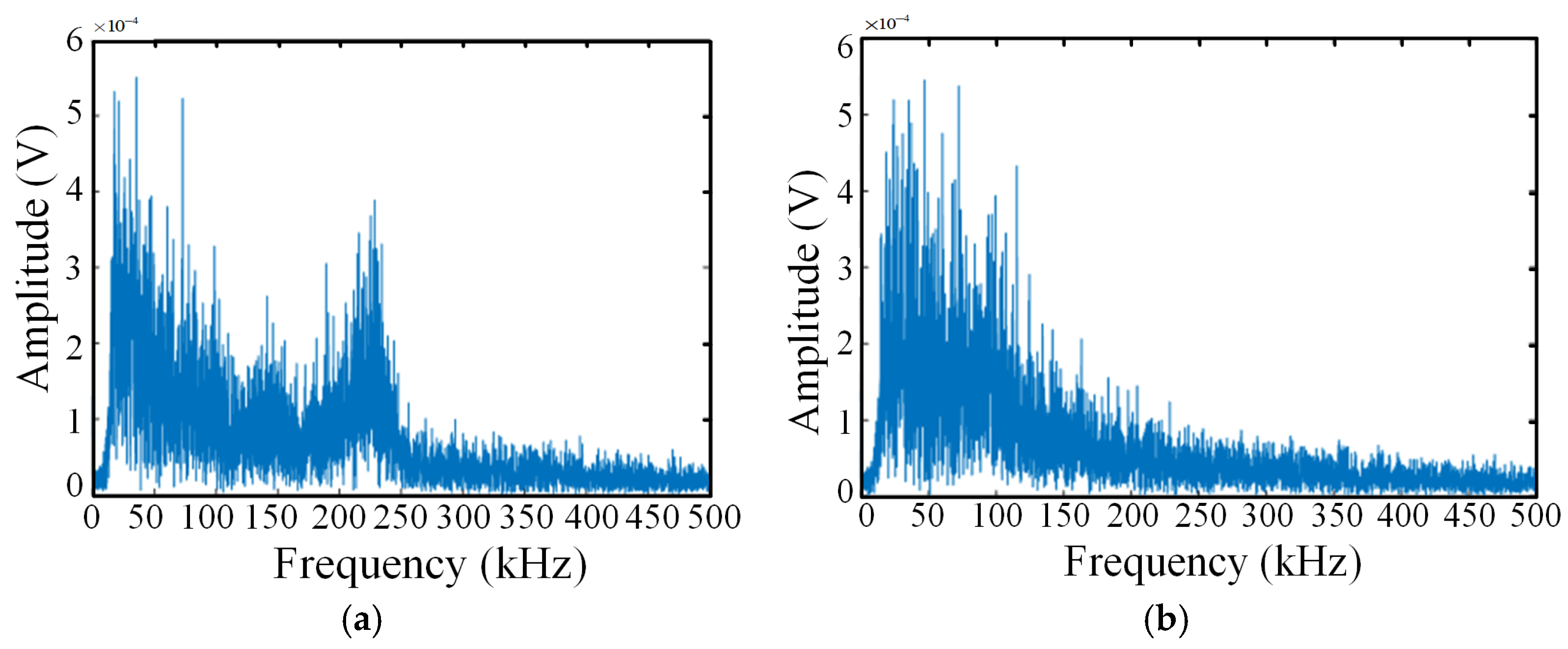
Similarly, frequency domain analysis was conducted on the noise signals from the testing platform, and the results are presented in Figure 5.

Comparative analysis of the results reveals that, in contrast to laboratory noise signals, the frequency distribution range of the platform noise signals is broader, the amplitudes are higher, and the signals are more complex. At the 19-m platform location, the noise is mainly distributed in the range of 0 to 260 kHz, with distinct peaks at 20 kHz and 227 kHz. In contrast, at the 29-m platform location, the noise is also predominantly distributed in the range of 0 to 260 kHz, but with only one peak. Combining the spectral graphs of leakage acoustic emission signals from the pipeline system under different pressures, it can be observed that the characteristic frequency range of the leakage acoustic emission signals overlaps with the actual noise signal frequencies. This overlap poses challenges to pipeline leak detection efforts.

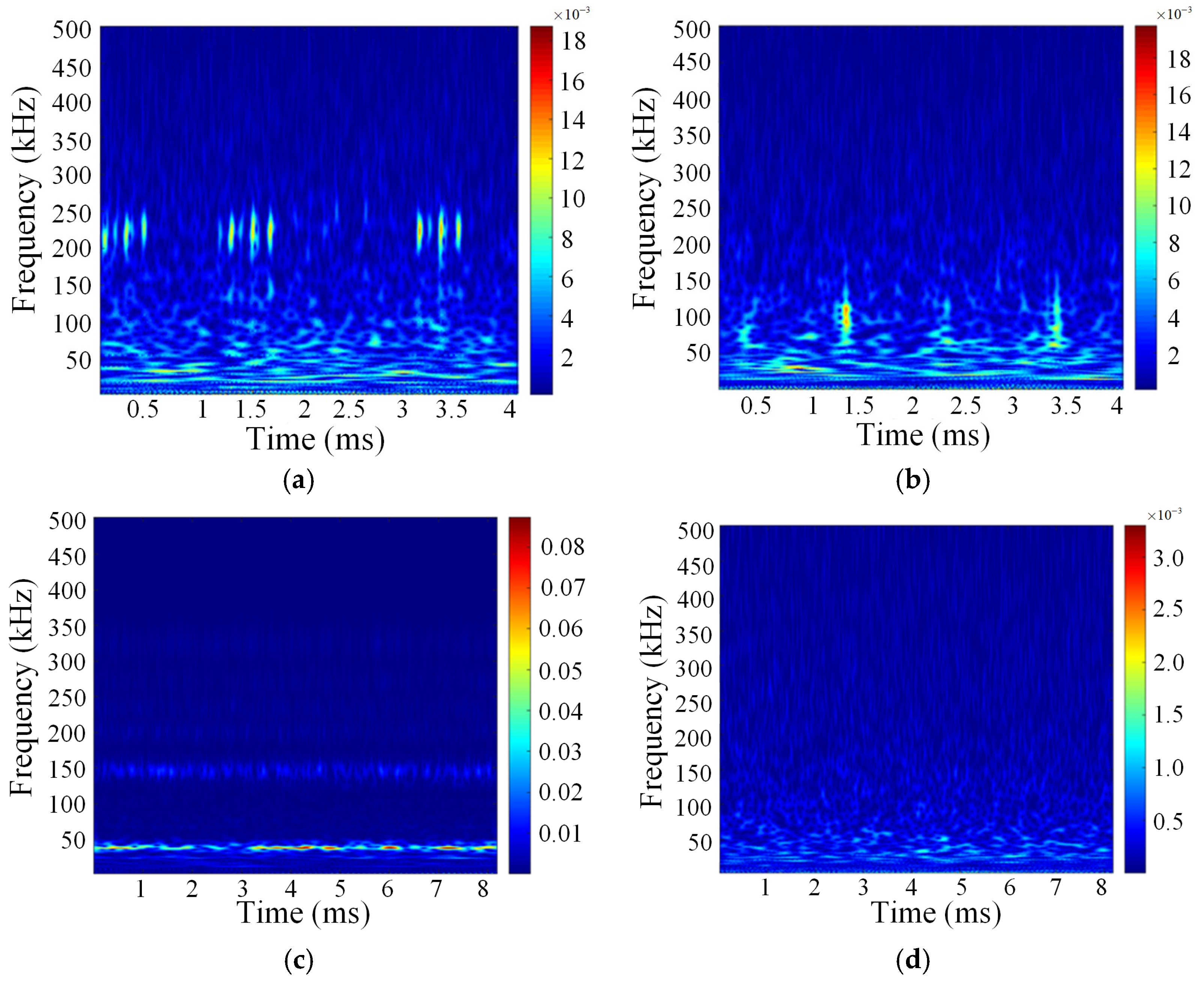
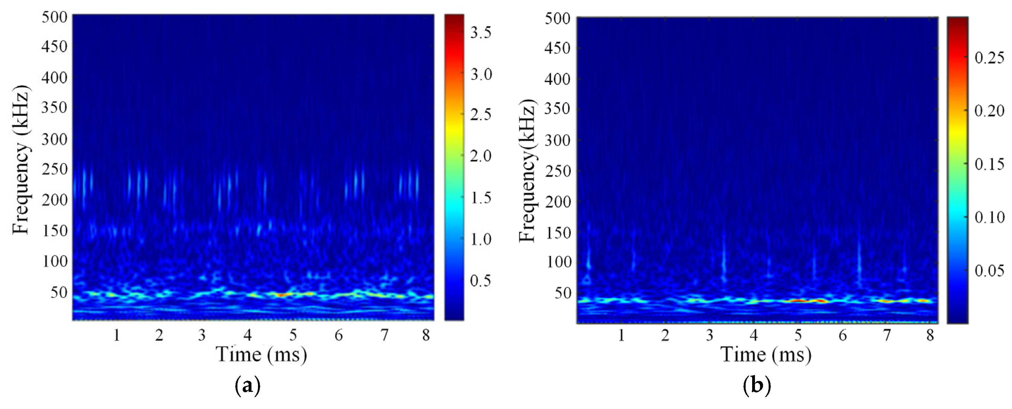
To further analyze the frequency distribution characteristics between leakage signals and environmental noise signals, a time–frequency analysis was conducted to more intuitively illustrate the relationship between the frequency amplitude of the signals and time. The analysis results are presented in Figure 6.

From the above analysis results, it is clear that the on-site noise has a broader frequency distribution range compared to laboratory noise, and the situation is more complex. The noise signals from the 19-meter and 29-meter platform pipelines consist mainly of two parts: one part is random noise concentrated in the range of 0 to 80 kHz, and the other part is periodic burst noise signals within the ranges of 180 to 250 kHz and 70 to 130 kHz, respectively. The frequency distribution of the noise signals obtained in the laboratory is in the range of 0 to 60 kHz, without burst signals and with lower amplitudes. The leakage acoustic emission signals obtained in the laboratory are mainly distributed in two frequency bands: 30 to 50 kHz and 135 to 165 kHz. There is frequency overlap with the measured noise signals, and if both occur simultaneously in a real leakage scenario, distinguishing between leakage and noise signals solely based on frequency domain information will become challenging.

Comparison reveals that the frequency range of leakage acoustic emission signals is more concentrated and significantly higher than that of noise signals in the same frequency band. Therefore, when a leakage occurs, the energy distribution of the acoustic emission signals will inevitably change. This provides a new research perspective and approach for extracting characteristic parameters of leakage signals.

2.3. Fusion of Leakage Signals and Measured Noise Signals

Due to the low noise level in the laboratory, it is unable to accurately reflect the actual noise conditions on offshore platforms. To simulate realistic environmental conditions, the measured noise signals from the platform were fused with the leakage acoustic emission signals collected in the laboratory. This fusion aimed to validate the pipeline leakage detection method based on acoustic emission technology. As both signals are continuous, the noise percentage was determined using signal power [41], i.e.,

$$\epsilon =\sqrt{\frac{P_N}{P_S}}=\sqrt{\frac{RM{S}_N^2}{RM{S}_S^2}}=\frac{RM{S}_N}{RM{S}_S}$$

(1)

In the above formula, P_N represents the noise power, P_S represents the signal power, and RMS_N and RMS_S are the root mean square values of the noise signal and leakage signal, respectively. Therefore, the combined leakage signal Y can be obtained by the following equation:

$$Y=X+\frac{RM{S}_S}{\epsilon \cdot RM{S}_N}Noise$$

(2)

In this equation, X represents the collected leakage signal, and Noise represents the measured noise signal.

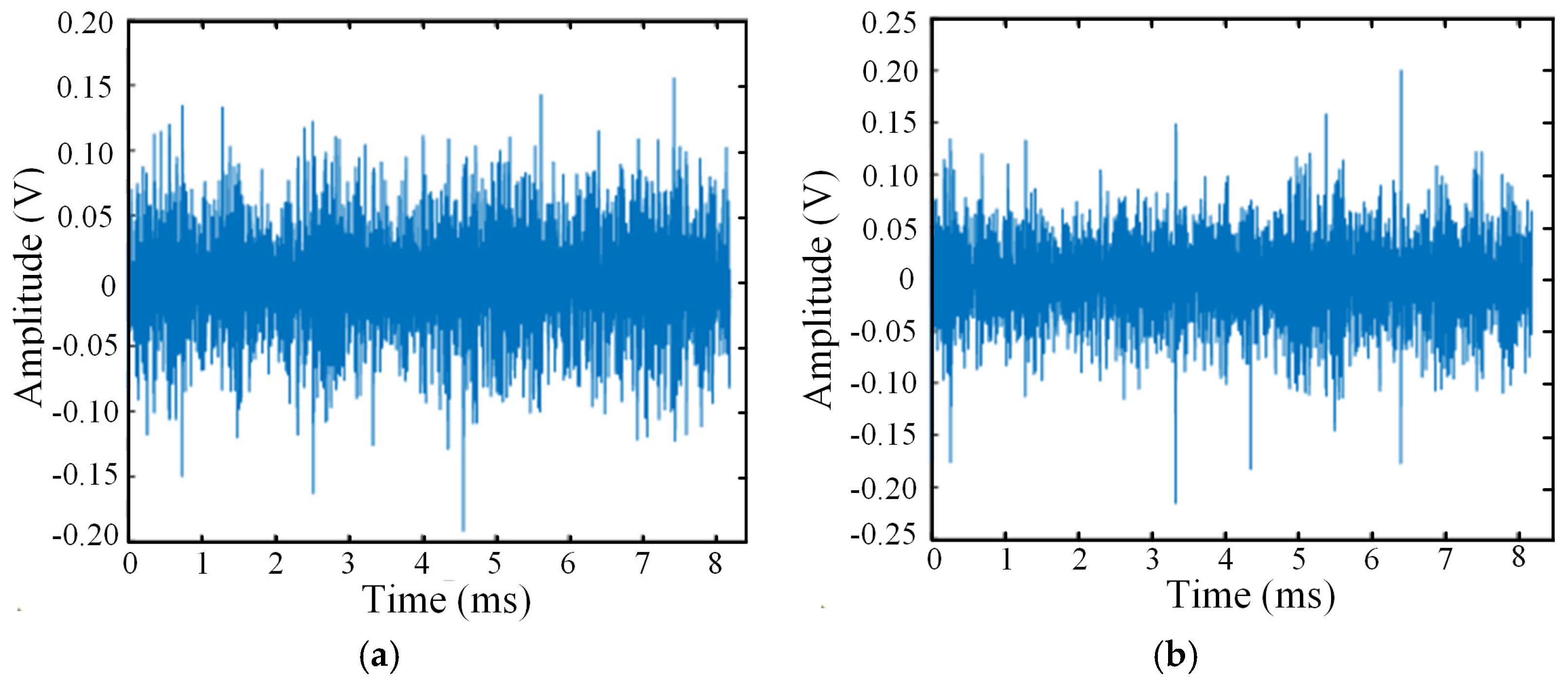
Due to the inconsistent noise characteristics at the 19-m and 29-m pipeline locations on the testing platform, they were separately injected into the leakage acoustic emission signals, resulting in 99 sets of leakage signals containing measured noise. The waveforms are shown in Figure 7.

The above analysis results indicate that, after incorporating measured noise, the leakage acoustic emission signals with noise differ significantly from those without noise, in terms of waveform. The results are more similar to the measured noise signal. Therefore, identifying measured leakage acoustic emission signals solely from a time–domain perspective is not advisable. 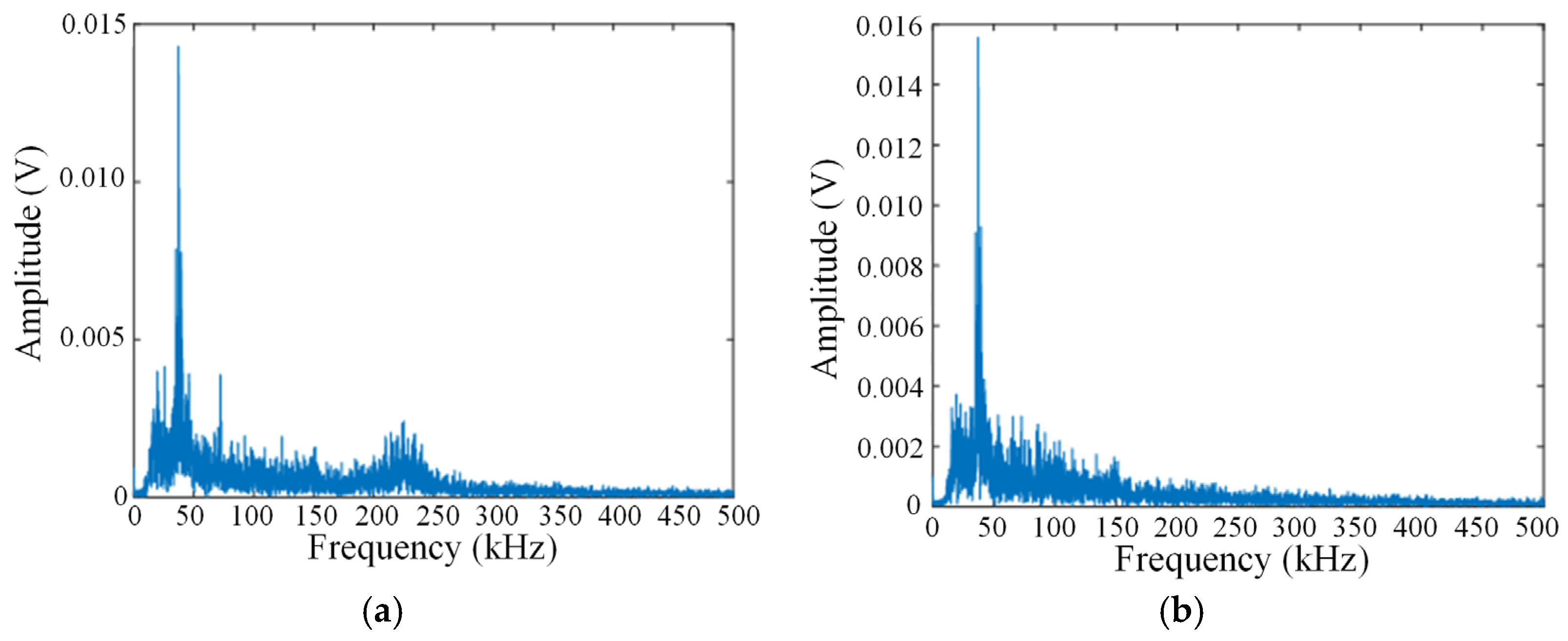Further frequency domain analysis was conducted on the noisy acoustic emission signals, and the results are shown in Figure 8.

To obtain more clear results, time–frequency analysis was performed on the noisy acoustic emission signals, and the outcomes are presented in Figure 9.

The spectrogram and time–frequency diagram of the signal with noise, the original leak acoustic emission signal, and the measured noise signal have undergone changes compared to each other. They now exhibit characteristics of both the laboratory leak acoustic emission signal and the measured noise signal. The peaks of the original leak acoustic emission signal at 15 kHz and 146 kHz are no longer prominent due to their smaller amplitudes. However, the peak at 36 kHz remains clearly observable and exhibits a continuous pattern in the time–frequency diagram. These changes lay the foundation for subsequent feature extraction and pattern recognition of leak acoustic emission signals.

3. Modal Decomposition Method for Leak Identification Analysis

3.1. Empirical Mode Decomposition Algorithm and Its Analysis Results

Empirical mode decomposition (EMD) is a method used for analyzing nonlinear and non-stationary signals. It decomposes signals based on the inherent timescale characteristics of the data without the need for predefined basis functions. The key to this method is empirical mode decomposition, which breaks down complex signals into a finite number of intrinsic mode functions (IMFs). Each IMF component extracted contains local characteristic signals of different time scales from the original signal. This approach allows for the stabilization of non-stationary data and subsequent Hilbert transform to obtain time–frequency spectrograms, revealing physically meaningful frequencies. Compared to methods like short-time Fourier transform and wavelet decomposition, EMD is adaptive as it decomposes signals based on the local properties of the signal sequence in the time domain.

Consider a signal $s\left(t\right)$, for which upper and lower envelope lines, denoted as $U_1\left(t\right)$ and $D_1\left(t\right)$ respectively, are derived by fitting its local maxima and minima. Subsequently, the mean value $M_1\left(t\right)$ of the signal is calculated:

$$M_1\left(t\right)=\frac{U_1\left(t\right)+D_1\left(t\right)}{2}$$

(3)

A new sequence $H_1\left(t\right)$ is obtained by subtracting the upper envelope line $M_1\left(t\right)$ from signal $s\left(t\right)$:

$$H_1\left(t\right)=s\left(t\right)-M_1\left(t\right)$$

(4)

Subsequently, it is necessary to assess if $H_1\left(t\right)$ satisfies the following two conditions:

(1)

The number of zero crossings should be equal to the number of extrema or differ by no more than one.

(2)

The upper and lower envelope lines should be locally symmetrical about the time axis, meaning the average values of the upper and lower envelope lines are zero.

If $H_1\left(t\right)$ meets the above conditions, it is considered a first order component. If not, the process is repeated until both criteria are met. If the standards are met after repeating the process k times, the first order component $C_1\left(t\right)$ can be expressed as:

$$H_{1k}\left(t\right)=H_{1\left(k-1\right)}\left(t\right)-M_{1k}\left(t\right)$$

(5)

$$C_1\left(t\right)=H_{1k}\left(t\right)$$

(6)

The separation of signal $C_1\left(t\right)$ from $s\left(t\right)$ results in the residual signal $R_1\left(t\right)$, as follows:

$$R_1\left(t\right)=s\left(t\right)-C_1\left(t\right)$$

(7)

In the equation, $R_1\left(t\right)$ represents the new signal to be decomposed. By repeating the aforementioned steps with signal $R_1\left(t\right)$, new IMF components can be obtained.

$$\left\{\begin{array}{c}{R}_1\left(t\right)-C_2\left(t\right)=R_2\left(t\right)\\ \begin{array}{c}\cdots \\ R_{n-1}\left(t\right)-C_n\left(t\right)=R_n\left(t\right)\end{array}\end{array}\right.$$

(8)

The above process is repeated for n iterations, and the decomposition stops when $R_n\left(t\right)$ becomes a monotonic function or its amplitude falls below a certain threshold. At this point, the original signal can be represented as the sum of n IMF components, denoted as $C_i(t)$, and a residual component $R_n\left(t\right)$:

$$s\left(t\right)={\displaystyle \sum _{i=1}^n{C}_i+R_n\left(t\right)}$$

(9)

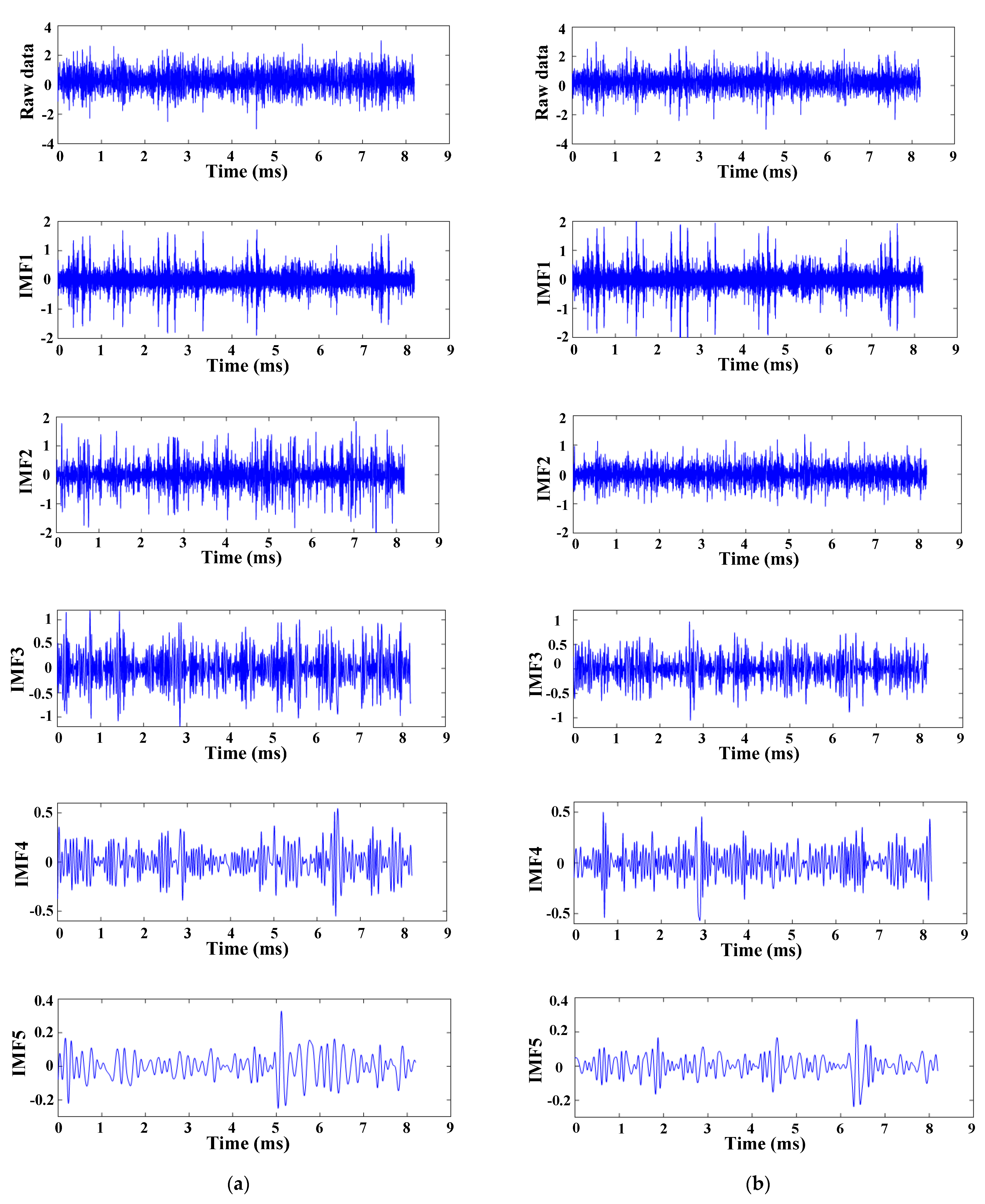
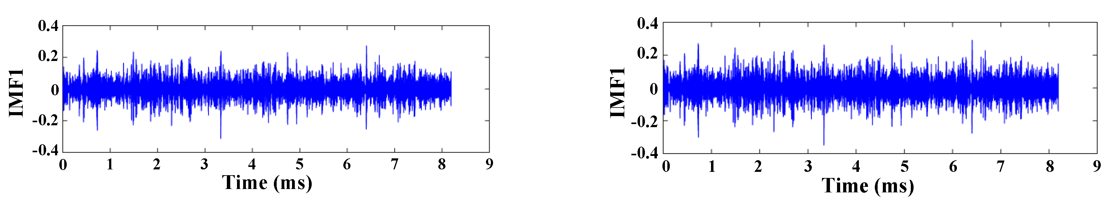
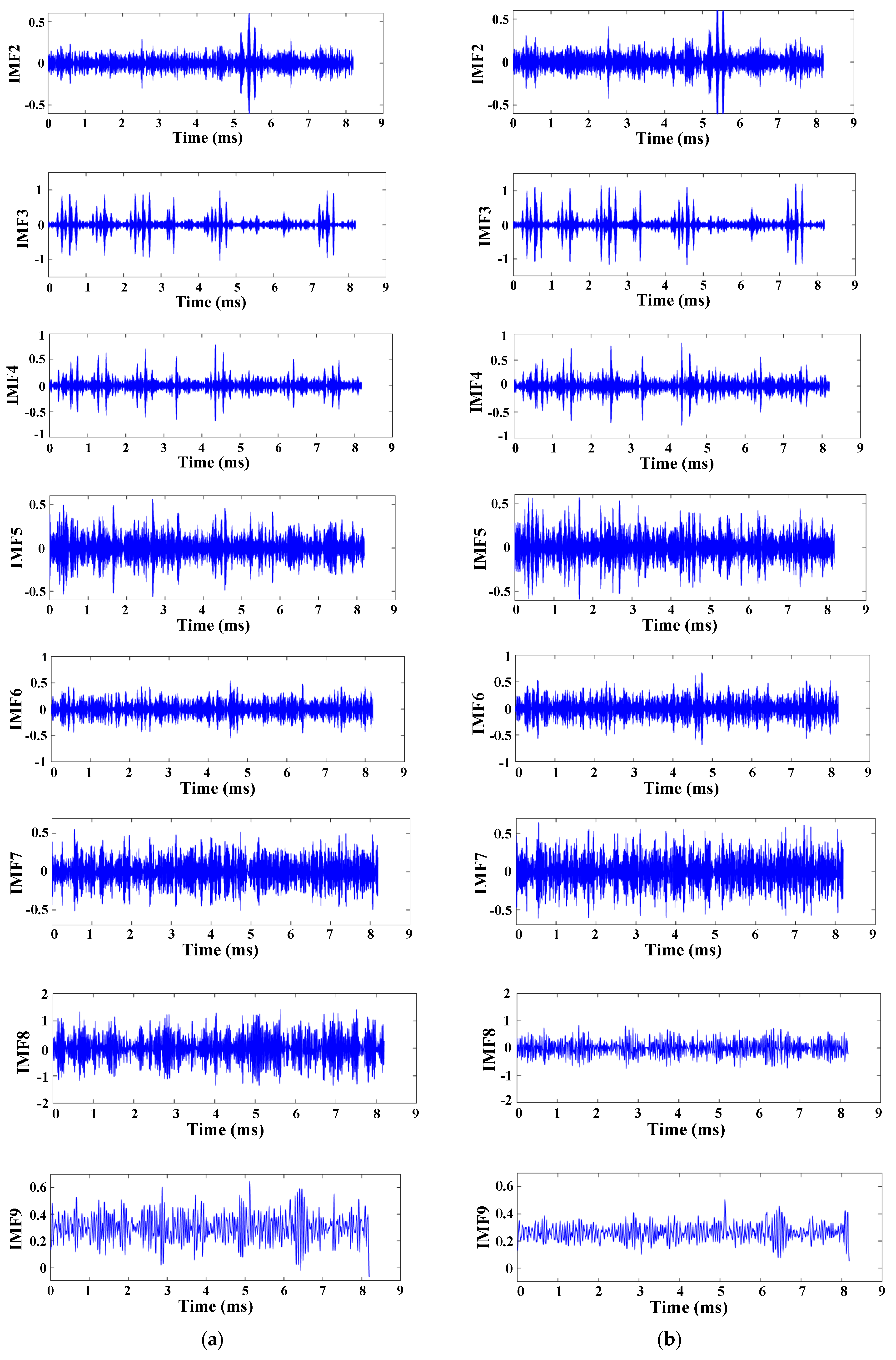
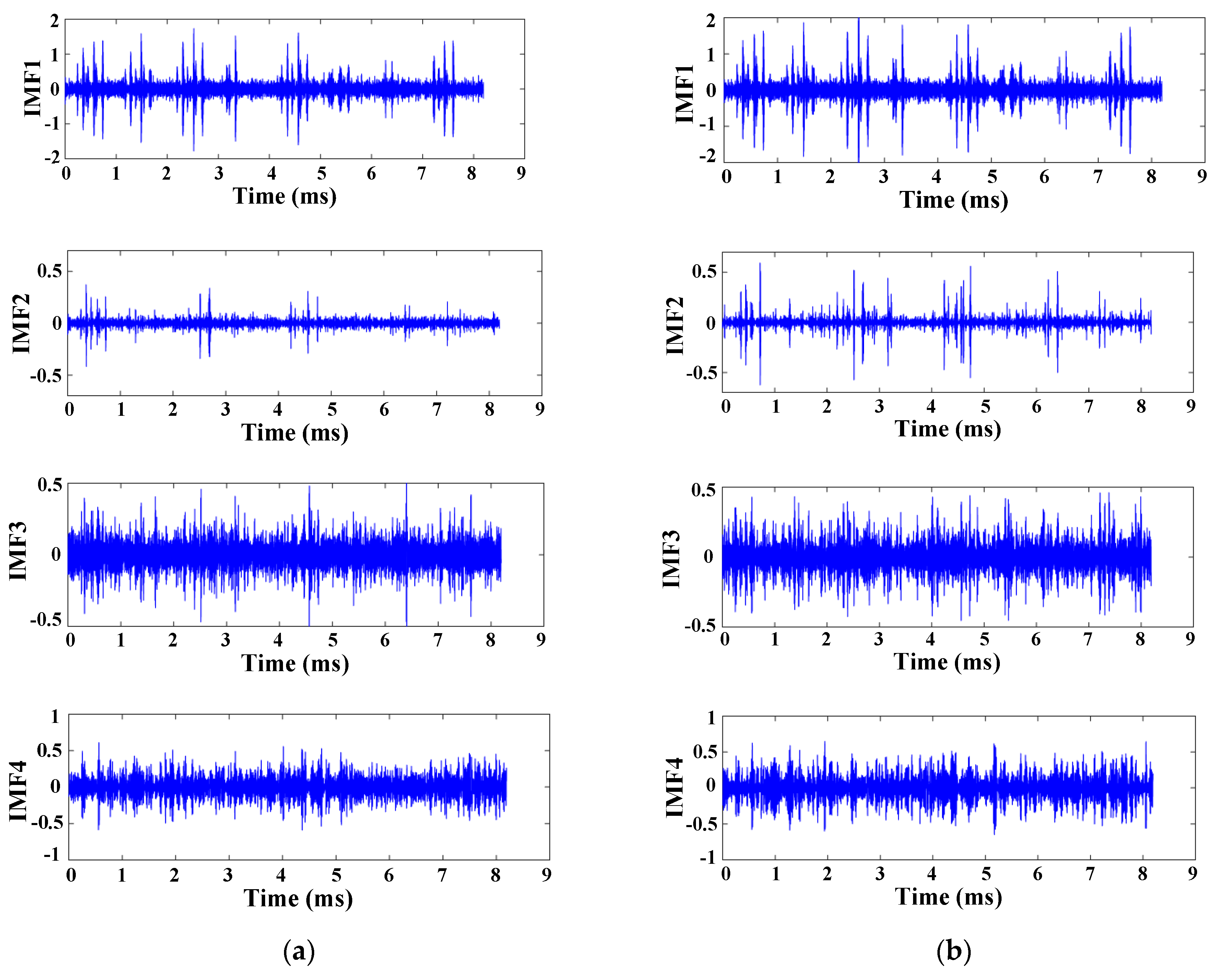
Collected acoustic emission signals were subjected to normalization, followed by the fusion of noise and leakage emission signals. The fused signal, along with the platform-measured noise signal, underwent EMD. Both signals were decomposed into 10th order components and 11th order components, with the final component representing the residual term. As the characteristic features of the decomposed signals primarily reside in the initial orders, a comparative analysis was performed on the decomposed signals up to the fifth order. The results are depicted In Figure 10.

The decomposition results reveal that, under the influence of noise interference, the leakage signal with noise and the measured noise signal exhibit minimal differences in the first order component, both showing sudden peaks at corresponding time points. In the second order component, the amplitude decay of the noise-added leakage signal is not significant, while the measured noise signal experiences considerable attenuation, compared to the first order component, with noticeable waveform differences. The third to fifth order components have similar amplitudes, but their amplitude arrival times vary. Subsequent components provide little useful information and are therefore not individually discussed.

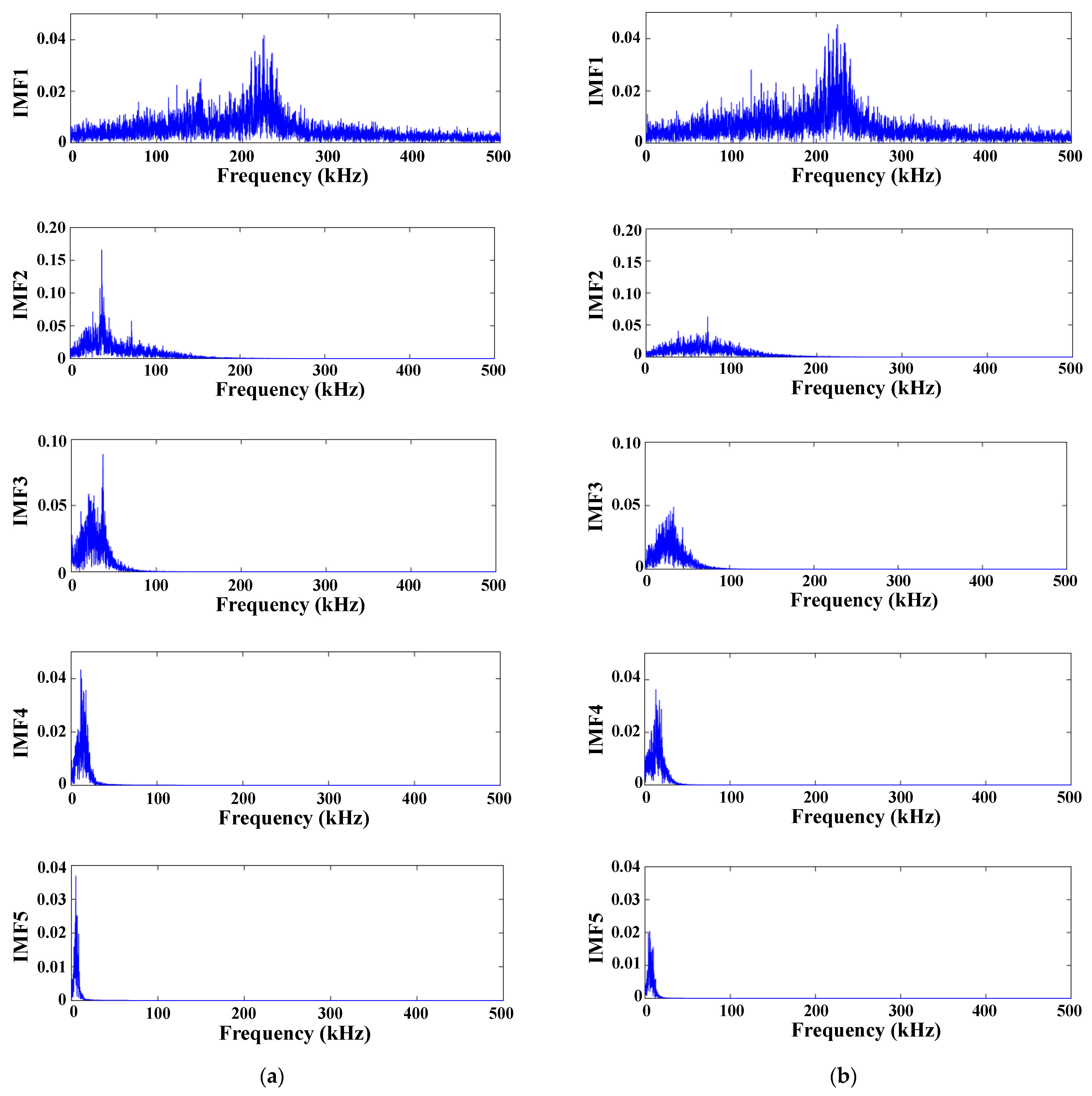
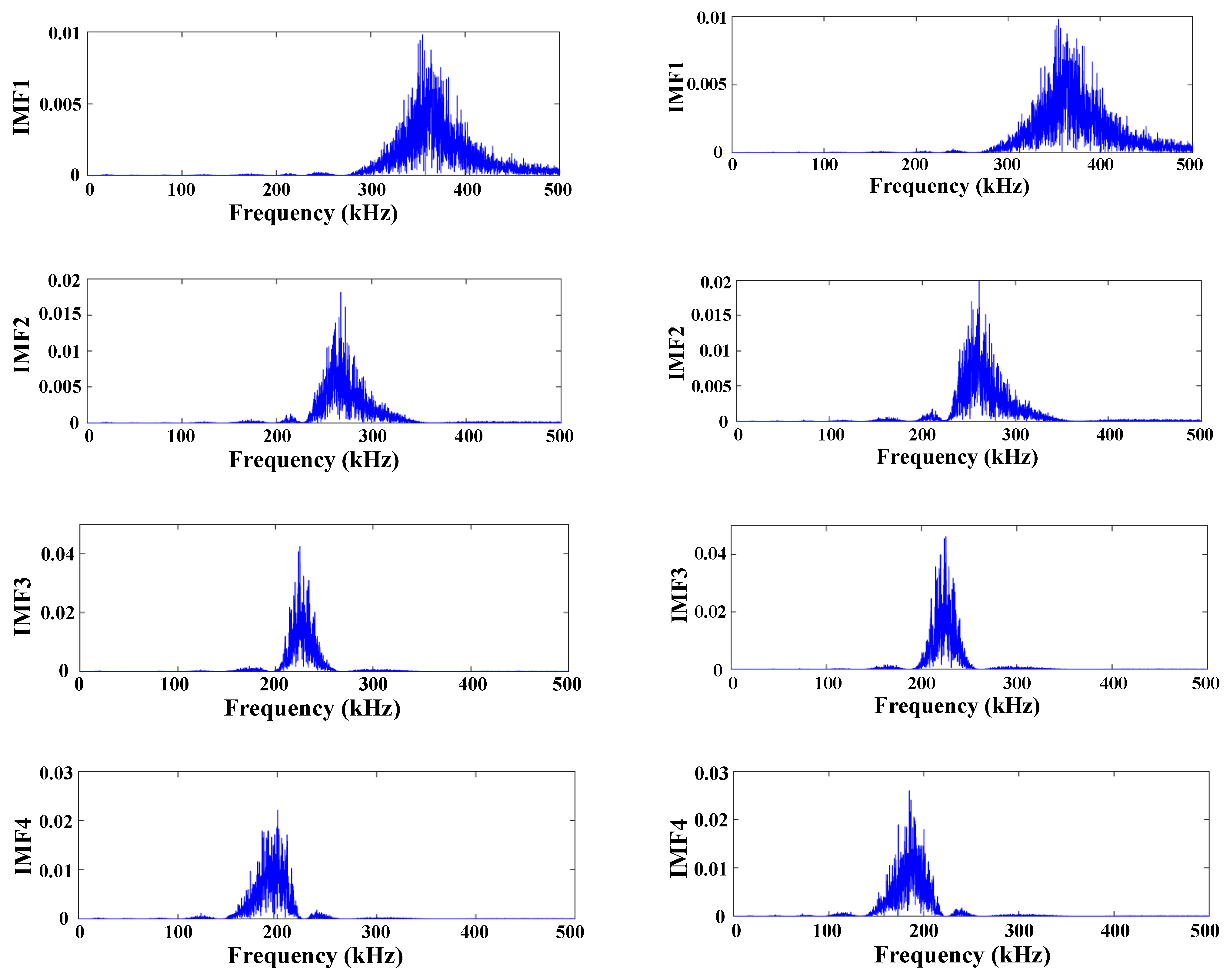
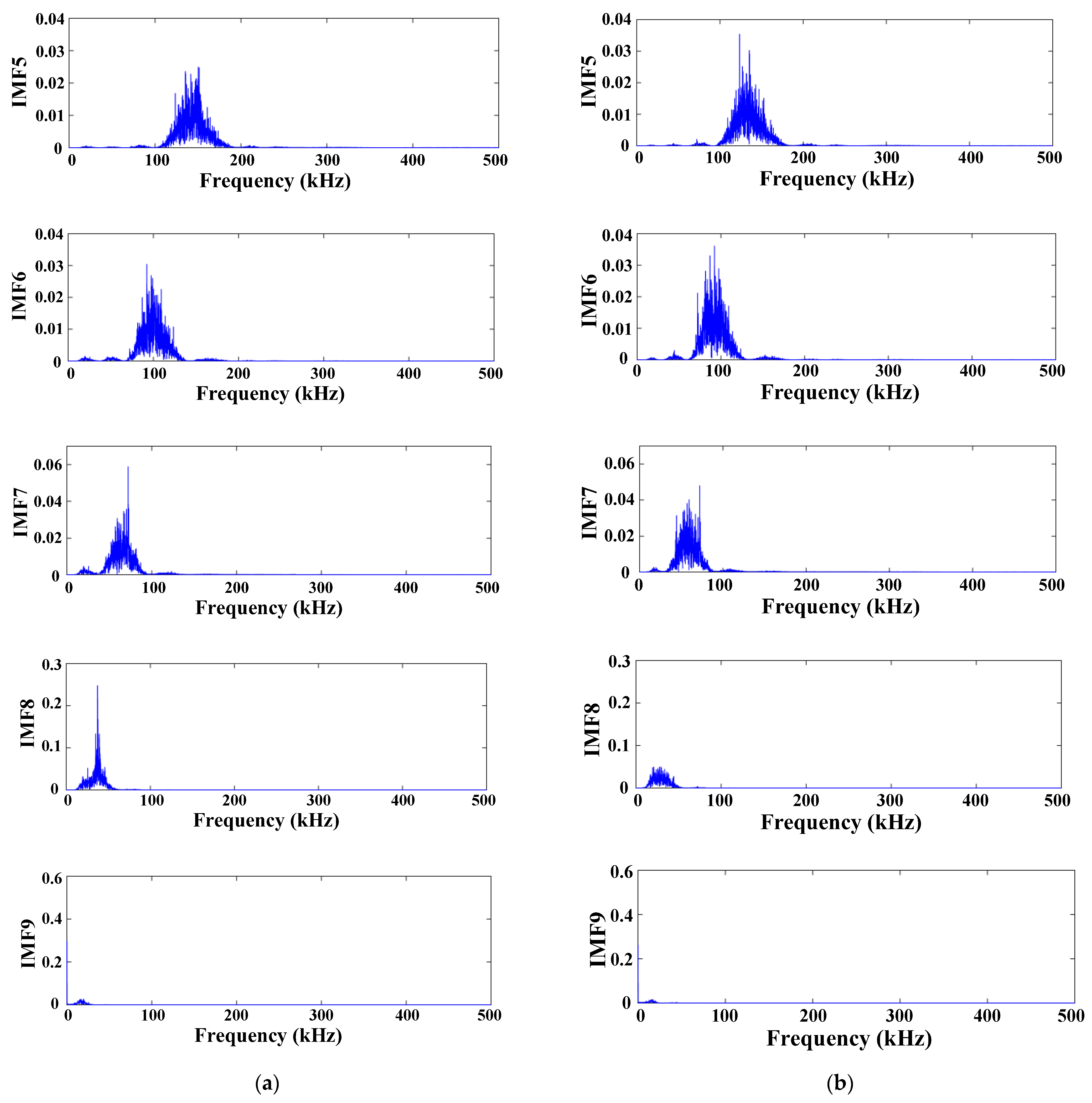
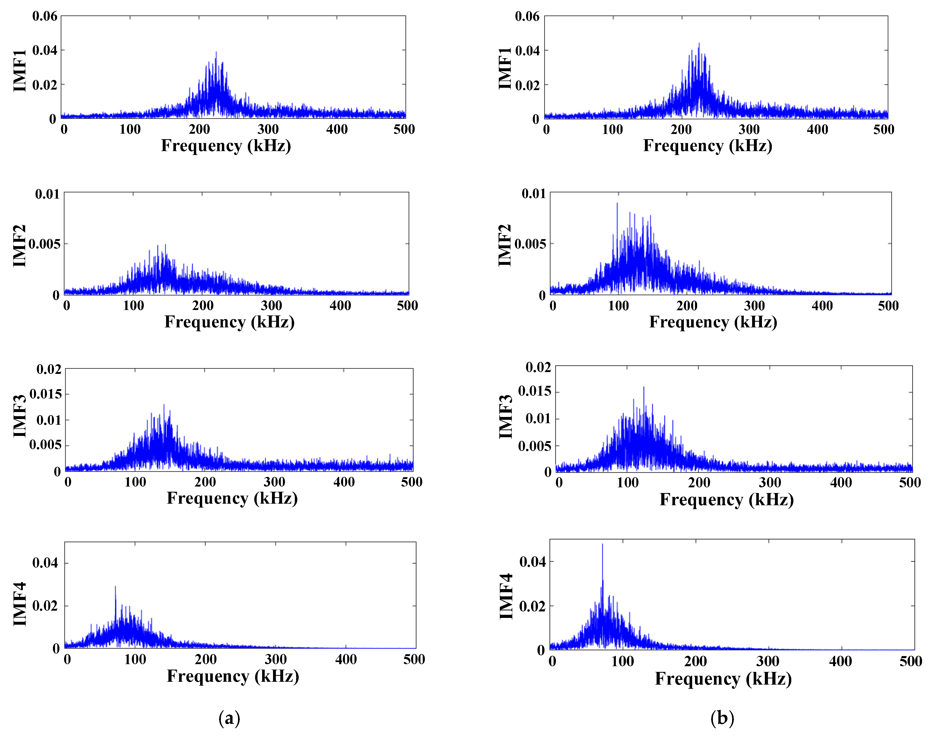
Subsequently, Fourier transforms were applied to the first five IMF components, and the frequency spectra are presented in Figure 11. It is observed that the frequencies of the components obtained from EMD decomposition overlap, and they are arranged in descending order. The spectra of the first components are remarkably similar, with peak frequencies appearing in the high frequency region, characteristic of noise signals. While the frequency distribution range of the second to fifth order components is consistent, the noise-added leakage signal exhibits higher peaks in these components, generally surpassing the amplitude of the measured noise signal.

In summary, the utilization of EMD provides some characteristic information. However, due to the high degree of overlap between the two signals, the distinction between leakage signals and noise signals is not sufficiently pronounced. This poses a certain challenge for subsequent feature extraction and pattern recognition.

3.2. Variational Mode Decomposition Algorithm and Its Analysis Results

Variational mode decomposition (VMD) is an adaptive and entirely non-recursive method for modal variation and signal processing. This technique offers the advantage of determining the number of modal decompositions. Its adaptability is manifested in determining the modal decomposition count of the given sequence based on actual conditions. During subsequent search and solving processes, it adaptively matches the optimal center frequency and limited bandwidth for each mode, and effectively separates the intrinsic mode functions (IMFs), divides the signal in the frequency domain, and ultimately obtains the effective decomposition components of the given signal. It achieves the optimal solution to the variational problem. VMD addresses issues present in EMD, such as endpoint effects and mode component overlap. Additionally, it boasts a more robust mathematical foundation, which aids in reducing the high complexity and strong nonlinearity of time series non-stationarity. The decomposition results in obtaining multiple sub-sequences with different frequency scales that are relatively stationary, making it suitable for non-stationary sequences. The core idea of the VMD algorithm is to construct and solve variational problems. The decomposition layer count k can be manually set, and the bandwidth of component $u_k$ is limited, with each center frequency being unique.

For each component $u_k$, a Hilbert transform is applied, yielding its one-sided spectrum and analytical signal A:

$$A=\left[\delta \left(t\right)+\frac{j}{\pi t}\right]u_k\left(t\right)$$

(10)

In the equation: $\delta \left(t\right)$ represents the impulse function.

Multiplying the above equation by the exponential function $e^{-j{\omega }_{k}t}$ yields the baseband signal, as follows:

$$B=\left[\left(\delta \left(t\right)+\frac{j}{\pi t}\right)u_k\left(t\right)\right]e^{-j{\omega }_{k}t}$$

(11)

Compute the L² norm of its gradient, square the result, and sum them up to obtain the bandwidths of each component. Simultaneously, it is essential to meet two criteria for VMD decomposition:

(1)

Minimize the bandwidth of the center frequency for each IMF component.

(2)

Ensure that the sum of all components equals the original signal.

$$s\left(t\right)={\displaystyle \sum _k{u}_k}\left(t\right)$$

(12)

In the equation: $s\left(t\right)$ denotes the initial signal, and $u_k\left(t\right)$ represents the k intrinsic mode functions obtained after decomposition.

$$\left\{\begin{array}{c}\underset{\left\{u_k\right\},\left\{{\omega }_k\right\}}{\min }\left\{{\displaystyle \sum _{\mathrm{k}}{‖{\partial }_t\left[\left.\left(\delta \left(t\right)+\frac{j}{\pi t}\right)u_k\left(t\right)\right]e^{-j{\omega }_{k}t}\right.‖}_2^2}\right\}\\ s.t.{\displaystyle \sum _k{u}_k=s\left(t\right)}\end{array}\right.$$

(13)

In the equation: $\left\{{\omega }_k\right\}=\left\{{\omega }_1,\cdots ,{\omega }_k\right\}$ represents the central frequency of each component after decomposition.

To obtain the optimal solution for Equations (3)–(11), it is necessary to introduce the extended Lagrange function:

$$\begin{array}{c}L\left(\left\{u_k\right\},\left\{{\omega }_k\right\},\lambda \right)=\alpha {\displaystyle \sum _k{‖{\partial }_t\left[\left(\delta \left(t\right)+\frac{j}{\pi t}\right)u_k\left(t\right)e^{-j{\omega }_{k}t}\right]‖}_2^2}\\ +{‖s\left(t\right)-{\displaystyle \sum _k{u}_k\left(t\right)}‖}_2^2+〈\lambda \left(t\right),s\left(t\right)-{\displaystyle \sum _k{u}_k\left(t\right)}〉\end{array}$$

(14)

In the equation: $\lambda$ is the Lagrange multiplier operator, and $\alpha$ is the quadratic penalty factor.

At this point, the constrained variational problem has been transformed into an unconstrained variational problem. The components and their central frequencies are updated using the alternating direction multiplier method:

$$\left\{\left.{\widehat{u}}_k^{n+1}\right\}\right.=\frac{\widehat{s}\left(t\right)-{\displaystyle \sum _{i<k}^K{\widehat{u}}_i^{n+1}\left(\omega \right)}-{\displaystyle \sum _{i>k}^K{\widehat{u}}_i^n\left(\omega \right)+\frac{{\widehat{\lambda }}^n\left(\omega \right)}{2}}}{1+2\alpha {\left(\omega -{\omega }_k^n\right)}^2}$$

(15)

In the equation: ${\widehat{u}}_k^{n+1}$, $\widehat{s}\left(t\right)$, and ${\widehat{\lambda }}^n$ denote the Fourier transforms of $u_k^{n+1}$, $s\left(t\right)$, and ${\lambda }^n$ respectively.

The operational process of the VMD algorithm is as follows:

(1)

Initialize $\left\{{\widehat{u}}_k^1\right\}$, $\left\{{\widehat{\omega }}_k^1\right\}$, ${\widehat{\lambda }}^1$;

(2)

Set the iteration count, n = n + 1, the loop begins;

(3)

Satisfy $\omega \ge 0$, update each ${\widehat{u}}_k$ according to Equations (3)–(13);

(4)

Update the center frequency ${\omega }_k$;

$${\omega }_k^{n+1}=\frac{{\displaystyle {\int }_0^{\infty }\omega {\left|{\widehat{u}}_k^{n+1}\left(\omega \right)\right|}^{2}d\omega }}{{\displaystyle {\int }_0^{\infty }{\left|{\widehat{u}}_k^{n+1}\left(\omega \right)\right|}^{2}d\omega }}$$

(16)

(5)

Update the Lagrange multipliers $\lambda$;

$${\widehat{\lambda }}^{n+1}\left(\omega \right)={\widehat{\lambda }}^n+\beta \left[\widehat{s}\left(\omega \right)-{\displaystyle \sum _{k=1}^K{\widehat{u}}_k^{n+1}\left(\omega \right)}\right]$$

(17)

Equation where: $\beta$ is the noise tolerance parameter.

(6)

Repeat steps (2) to (5) until the termination condition is met:

$${\displaystyle \sum _{k=1}^K\left(\frac{{‖{\widehat{u}}_k^{n+1}-{\widehat{u}}_k^n‖}_2^2}{{‖{\widehat{u}}_k^n‖}_2^2}\right)}<\epsilon$$

(18)

In the equation, where: $\epsilon$ is the discrimination accuracy, and $\epsilon >0$.

Before performing VMD decomposition, modal parameters K and penalty factor $\alpha$ need to be pre-set. The modal parameter K is primarily used to control the number of decomposition layers; if it is too small, it may result in insufficient decomposition and modal aliasing, leading to under-decomposition. If it is too large, it may cause excessive decomposition, generating some useless components. The penalty factor $\alpha$ is used to control the bandwidth of the IMF components; if it is too large, it may cause some components to include others, while if it is too small, it may result in the loss of certain signals.

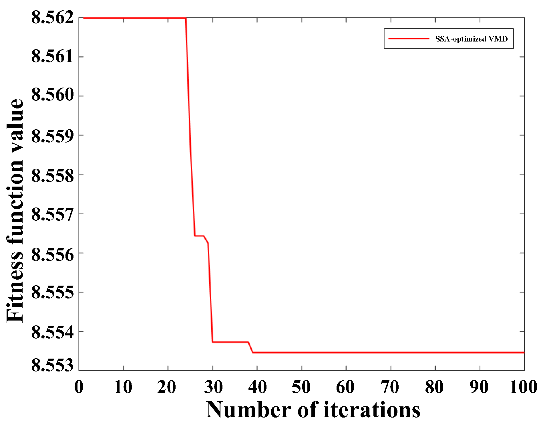
In this study, the Sparrow algorithm was employed to find the optimal modal parameters K and penalty coefficient a before VMD decomposition. The population size was set to 10, and the maximum number of iterations was set to 100. Modal parameter K was taken as $\left[3,20\right]$, and penalty coefficient a was taken as $\left[500,2500\right]$, with envelope entropy as the fitness function for the Sparrow optimization algorithm. The trend of envelope entropy changes during iterations is illustrated in Figure 12. After 39 iterations, the minimum envelope entropy value of 8.5535 was achieved and remained stable thereafter, resulting in the optimized values of $\left[k,\alpha \right]=\left[9,853\right]$.

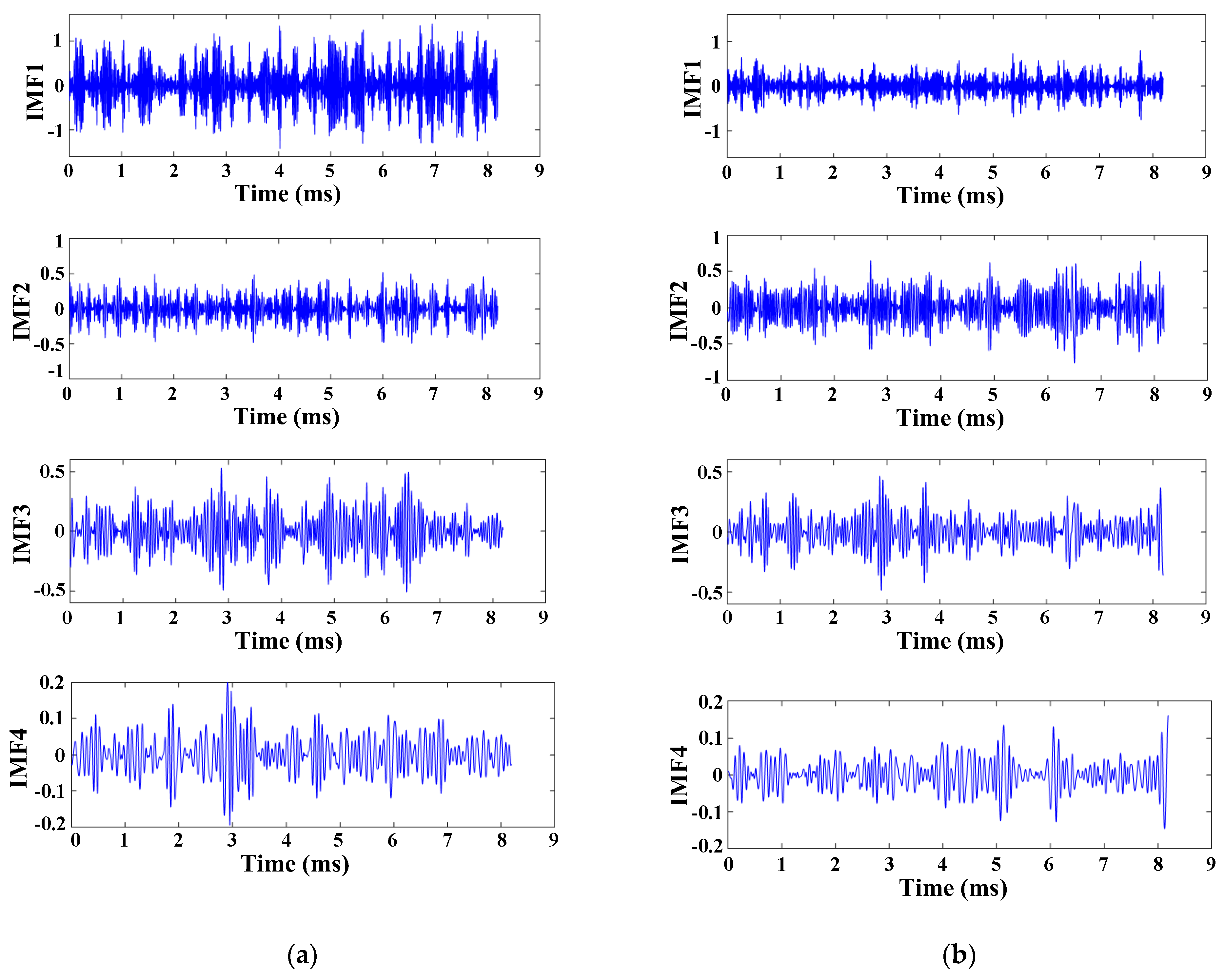
Based on the aforementioned preprocessing results, VMD decomposition was applied to the noisy leakage signal and platform noise signal, resulting in nine-order IMF components, as shown in Figure 13. It can be observed that, in the first four components, there is no significant difference between the noisy leakage signal and the measured noise signal. The waveforms and peak occurrence times are highly similar. The fifth component reveals differences between the two signals, with variations in the density of sudden peaks. The sixth and seventh components exhibit similarity once again. Moving to the eighth component, the amplitude of the noisy leakage signal is significantly higher than that of the noise signal, and their waveforms differ, indicating that the leakage signal contains more information. The ninth component represents the residual of the signal decomposition, and while the waveforms of the two signals are similar, the amplitude of the leakage signal is slightly higher.

After the VMD decomposition, each order signal possesses a unique central frequency. Extracting the central frequencies from the noisy leakage signals and the measured noisy signals, the results are presented in

Table 2. Center frequencies of IMF components (kHz).

IMF Components	Leakage Signals	Noise Signals	IMF Components	Leakage Signals	Noise Signals
IMF1	365.36	367.88	IMF6	98.94	91.60
IMF2	268.47	261.69	IMF7	65.24	58.86
IMF3	226.82	223.59	IMF8	37.10	28.57
IMF4	195.75	186.93	IMF9	0.79	0.32
IMF5	147.10	133.35

. It can be observed that the central frequencies corresponding to the significantly different fifth and eighth order components precisely fall within the characteristic frequency bands of the leakage signals. Moreover, there is no occurrence of closely spaced central frequencies in the leakage signals, indicating a thorough decomposition without excessive splitting.

Subsequently, each component underwent Fourier transformation to obtain the corresponding spectrum, and the analysis results are depicted in Figure 14.

It is evident that after VMD decomposition, the first order component shows minimal variation. Among the second to sixth orders, the peak values of the measured noise signal exceed those of the noisy leakage signal; however, in the seventh order, the peak of the leakage signal surpasses that of the measured noise signal yet, overall, the shapes of the main bodies in the first seven orders are relatively similar. In the eighth order, the peak of the leakage signal is much higher than that of the measured noise signal, and the two exhibit significant differences in shape. The ninth order component fails to provide meaningful information.

Overall, the VMD decomposition demonstrates superior performance, compared to EMD decomposition, revealing more distinct differences among the components. However, it should be noted that VMD decomposition requires preprocessing of the signal, making the analysis process more intricate than that of EMD decomposition.

3.3. Complete Ensemble Empirical Mode Decomposition with Adaptive Noise Algorithm and Its Analysis Results

The complete ensemble empirical mode decomposition with adaptive noise (CEEMDAN) algorithm is an improvement upon the ensemble empirical mode decomposition (EEMD), which is based on the EMD algorithm. This algorithm introduces complementary noise, significantly eliminating redundant noise during signal reconstruction without the need for hundreds of EMD decompositions, thereby greatly enhancing computational efficiency.

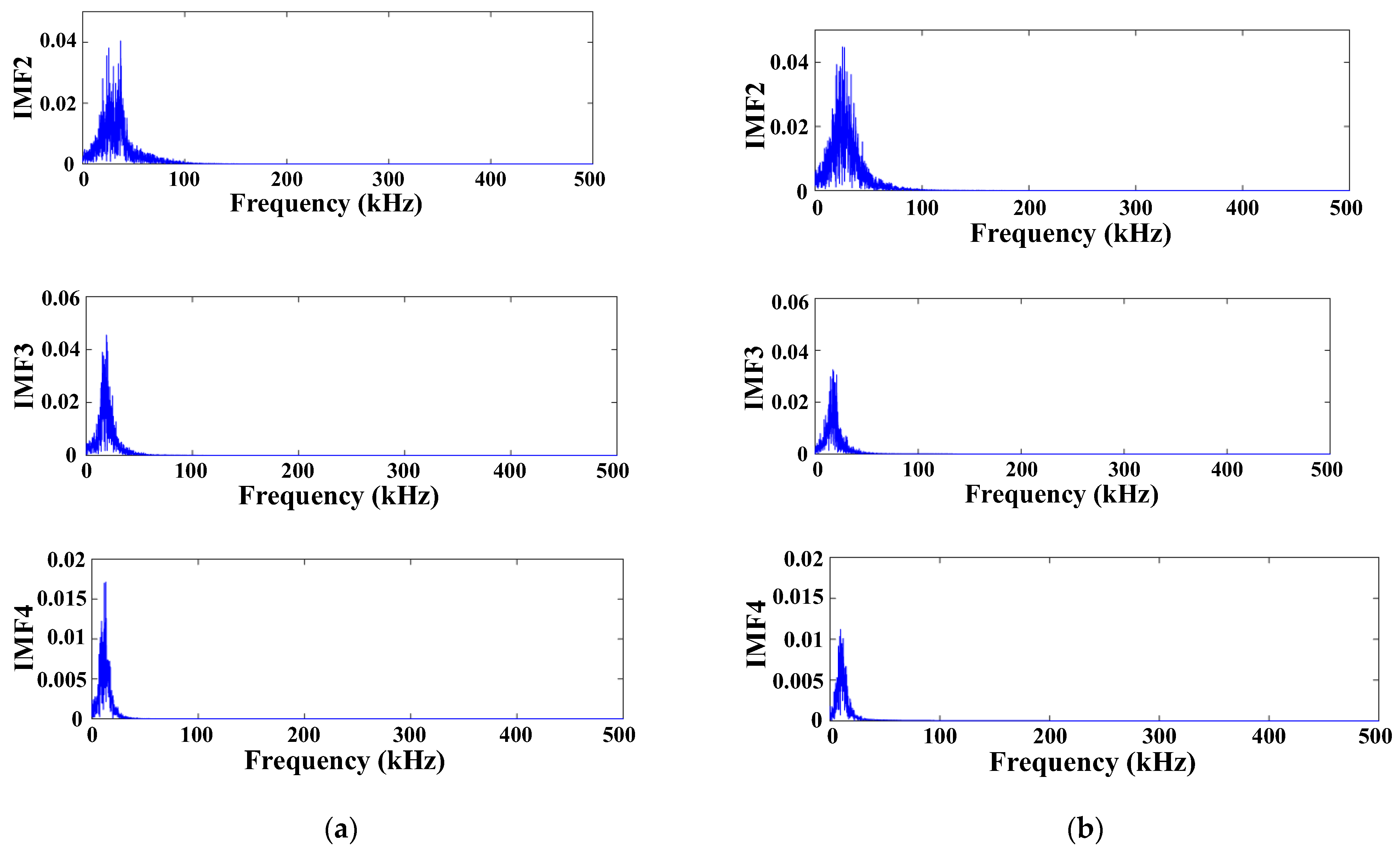
Since CEEMDAN is an enhancement of the EMD decomposition, it inherits the adaptive nature of the EMD algorithm, eliminating the need to set decomposition levels. With a white noise intensity set at 0.2, 50 iterations, and a maximum envelope iteration of 1000 for CEEMDAN decomposition, both the noisy leakage component and the noise component were obtained at the 14th order. 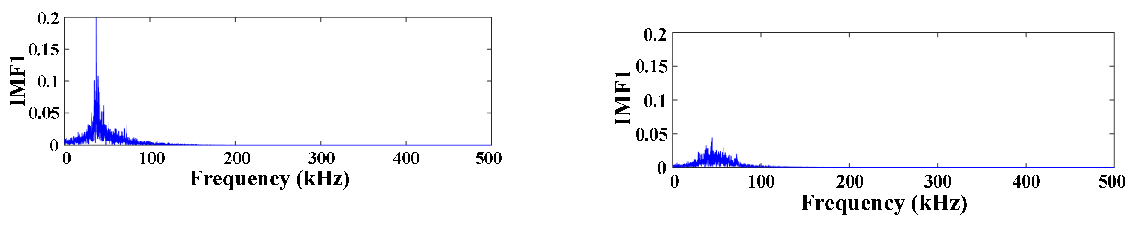As the signal characteristics primarily lie within the first four orders, these components were extracted, as shown in Figure 15. The decomposition results reveal a strong resemblance between the two signals in the first order component, with consistent peak values and occurrence moments of sudden peaks. In the second order component, the noise signal contains more sudden peaks with higher amplitudes. The third and fourth order components exhibit similar behavior, but the amplitude of the leakage signal is slightly higher than that of the noise signal.

After performing Fourier transformation on its components, the overall spectrum of each component appears to be arranged from high to low frequencies. The results are illustrated in Figure 16. The frequency distribution shapes of the first four order components are similar, with the amplitude of the noise signal component slightly higher than that of the leakage signal component overall.

Therefore, compared to EMD decomposition, CEEMDAN decomposition extracts more useful information. In comparison with VMD decomposition, CEEMDAN decomposition is more convenient, as it does not require pre-processing of the data.

4. Leakage Identification Analysis of the Improved Modal Decomposition Method

4.1. ICEEMDAN Algorithm and Its Analysis Results

Improved complete ensemble empirical mode decomposition with adaptive noise (ICEEMDAN) is an advanced signal processing algorithm that provides a more accurate and robust way to analyze complex signals. Developed as an enhancement of the EMD technique, ICEEMDAN builds upon the foundation of the CEEMDAN.

Distinguished from the CEEMDAN algorithm, ICEEMDAN exhibits essential differences in its computation. ICEEMDAN utilizes an advanced adaptive noise processing mechanism, effectively suppressing noise interference in signal decomposition. This mechanism dynamically adjusts filter parameters based on the real-time characteristics of the signal, adapting to both the signal’s spectrum and the temporal variability of noise. Consequently, ICEEMDAN not only accurately extracts the essential components of the signal but is also immune to external noise interference. ICEEMDAN avoids the direct addition of Gaussian white noise during the decomposition process. Instead, it selects the kth IMF component obtained after decomposing white noise, using EMD for analysis. This approach does not only alleviate the mode-mixing phenomenon present in traditional EMD methods but also addresses issues such as residual noise and pseudo-modes in the CEEMDAN method. Additionally, the method enables the ensemble averaging of multiple noise perturbations, resulting in more accurate decomposition outcomes and improved noise suppression capabilities. The ICEEMDAN decomposition results and spectrogram of ICEEMDAN decomposition components are shown in Figure 17 and Figure 18, respectively.

In the first order component, the amplitude of the leakage signal is significantly higher than that of the noise signal, with distinct differences in waveform shape and peak occurrence time. In the second to fourth order components, the magnitudes of the two signals are comparable, but there are noticeable differences in the arrival times of the waveforms.

In the first order component, the amplitude of the leakage signal is significantly higher than that of the noise signal. In the second order component, the two are generally similar, but the leakage signal has an additional peak frequency, compared to the noise signal. In the third and fourth order components, the frequency distribution and shape are similar for both, but in the third order component, the peak frequency of the leakage signal is slightly higher than that of the noise signal.

4.2. Comparative Analysis of Identification Results

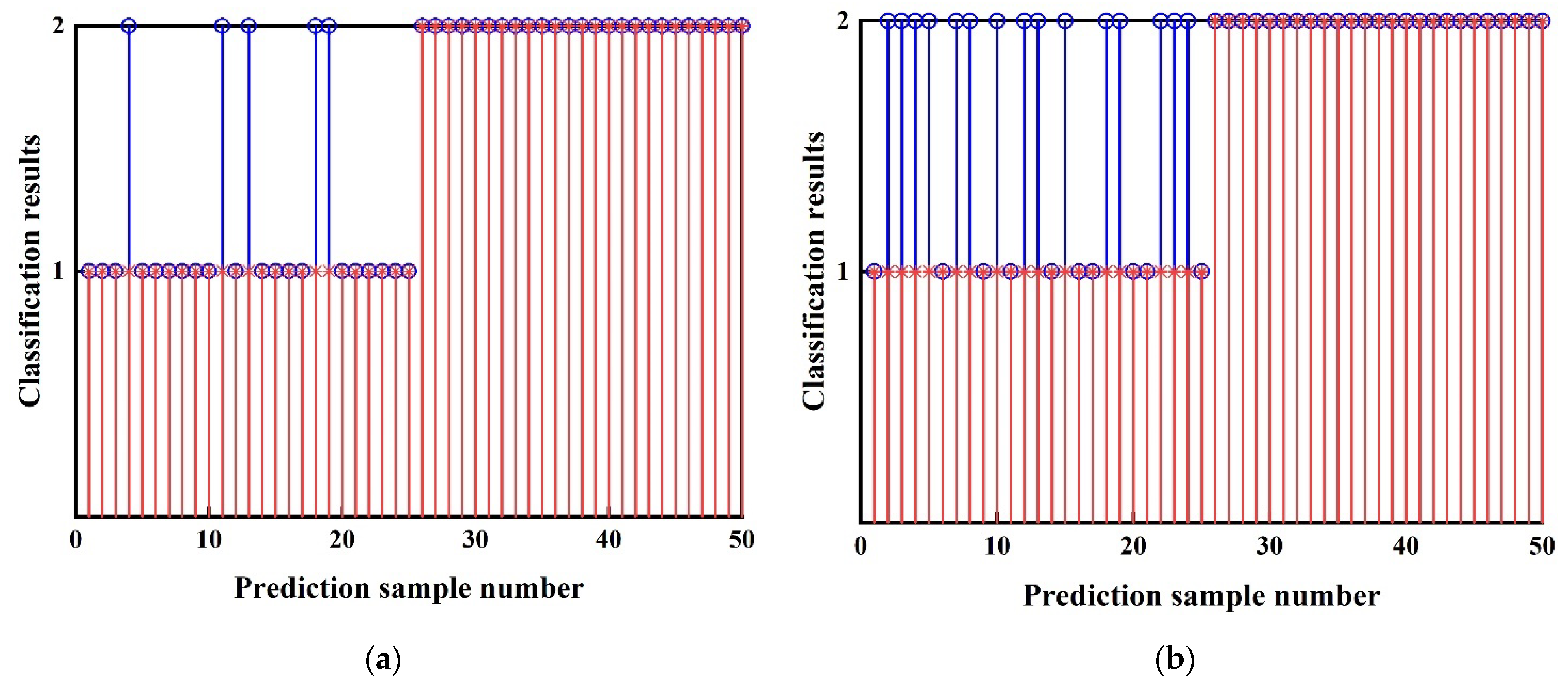
The recognition results of the feature vectors extracted by EMD are shown in Figure 19. Figure 19a displays the identification results for the non-fused noisy signal, while Figure 19b presents the identification results for the fused noisy signal.

The above analysis indicates that without incorporating noise, the EMD decomposition algorithm misidentifies five leakage signals as noise signals, achieving an accuracy of 90%. However, when the leakage signals are blended with noise signals, the EMD decomposition algorithm misidentifies 15 leakage signals as noise signals, resulting in an accuracy of only 70%. Therefore, it can be observed that the method based on EMD decomposition can to some extent distinguish between leakage and noise signals. However, it is highly sensitive to noise signals and is ineffective in extracting characteristic signals under low signal-to-noise ratio conditions.

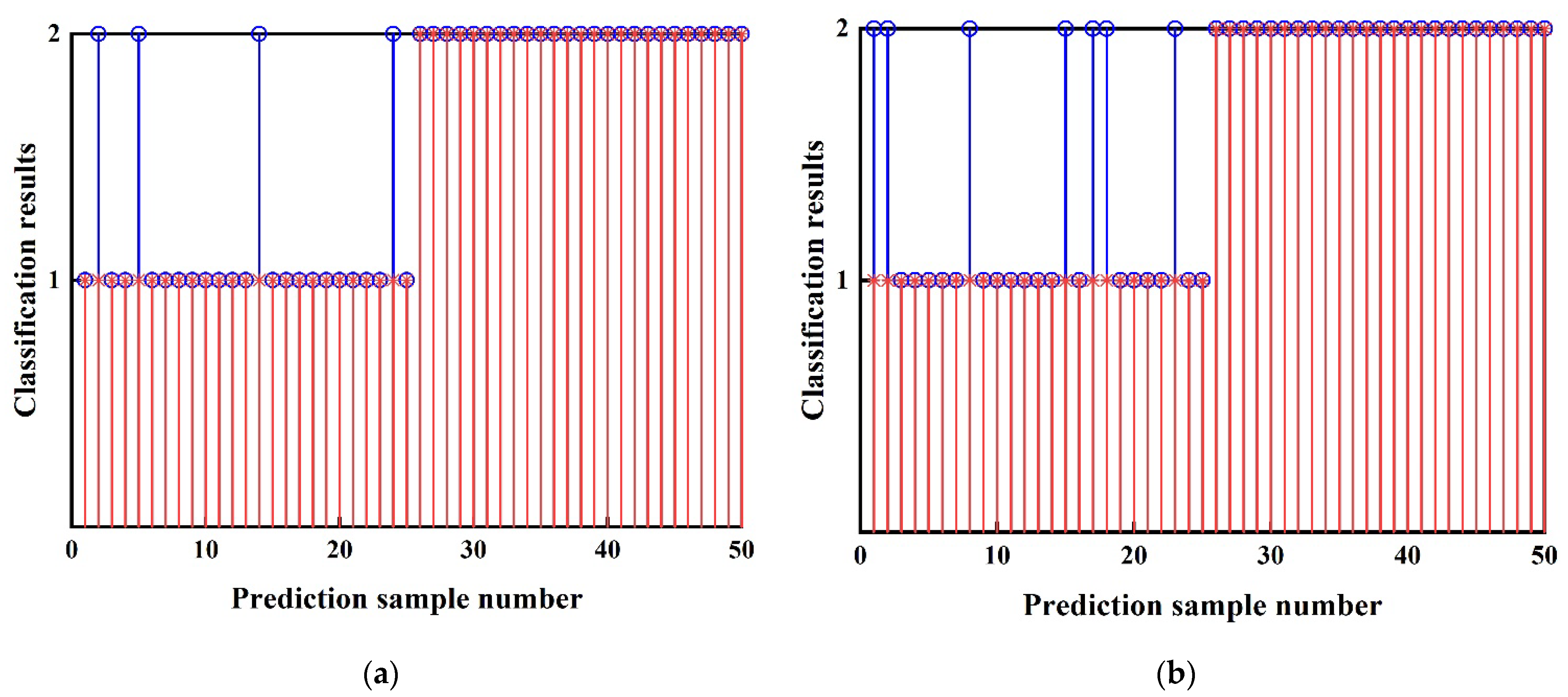
The recognition results of the feature vectors extracted using VMD are illustrated in Figure 20. Figure 20a represents the recognition results without integrated noise signals, while Figure 20b depicts the recognition results with integrated noise signals.

The analysis results above reveal that, without the inclusion of noise signals, the VMD decomposition algorithm correctly identified four leakage signals as noise signals, with an accuracy of 92%. When the leakage signals were integrated with noise signals, the VMD decomposition algorithm identified seven leakage signals as noise signals, achieving an accuracy of 86%. Thus, it can be observed that the method combining VMD decomposition with PNN performs slightly better in distinguishing leakage from noise signals, compared to the EMD combined with PNN method. Additionally, it exhibits superior resistance to noise interference than the EMD combined with PNN method.

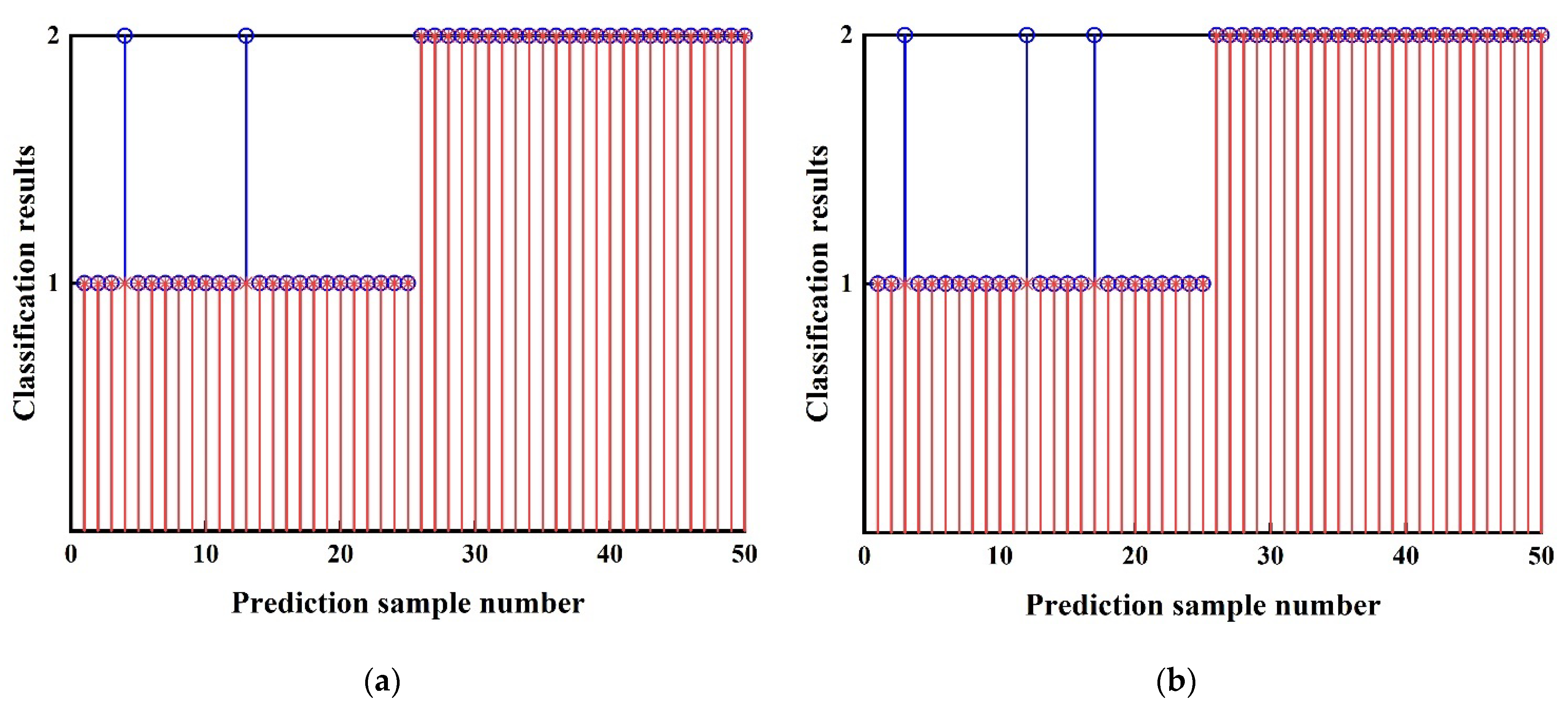
The recognition results of the feature vectors extracted based on CEEMDAN are depicted in Figure 21. Figure 21a represents the recognition results without integrated noise signals, while Figure 21b illustrates the recognition results with integrated noise signals.

The analysis results above indicate that, without the inclusion of noise, the CEEMDAN decomposition algorithm correctly identified two leakage signals as noise signals, achieving an accuracy of 96%. When the leakage signals were integrated with noise, the CEEMDAN decomposition algorithm identified three leakage signals as noise signals, with an accuracy of 94%. Hence, it can be observed that the method combining CEEMDAN decomposition with PNN performs slightly better in distinguishing leakage from noise signals, compared to the methods combining EMD and VMD with PNN. Additionally, it exhibits superior resistance to noise interference than the methods combining EMD and VMD with PNN.

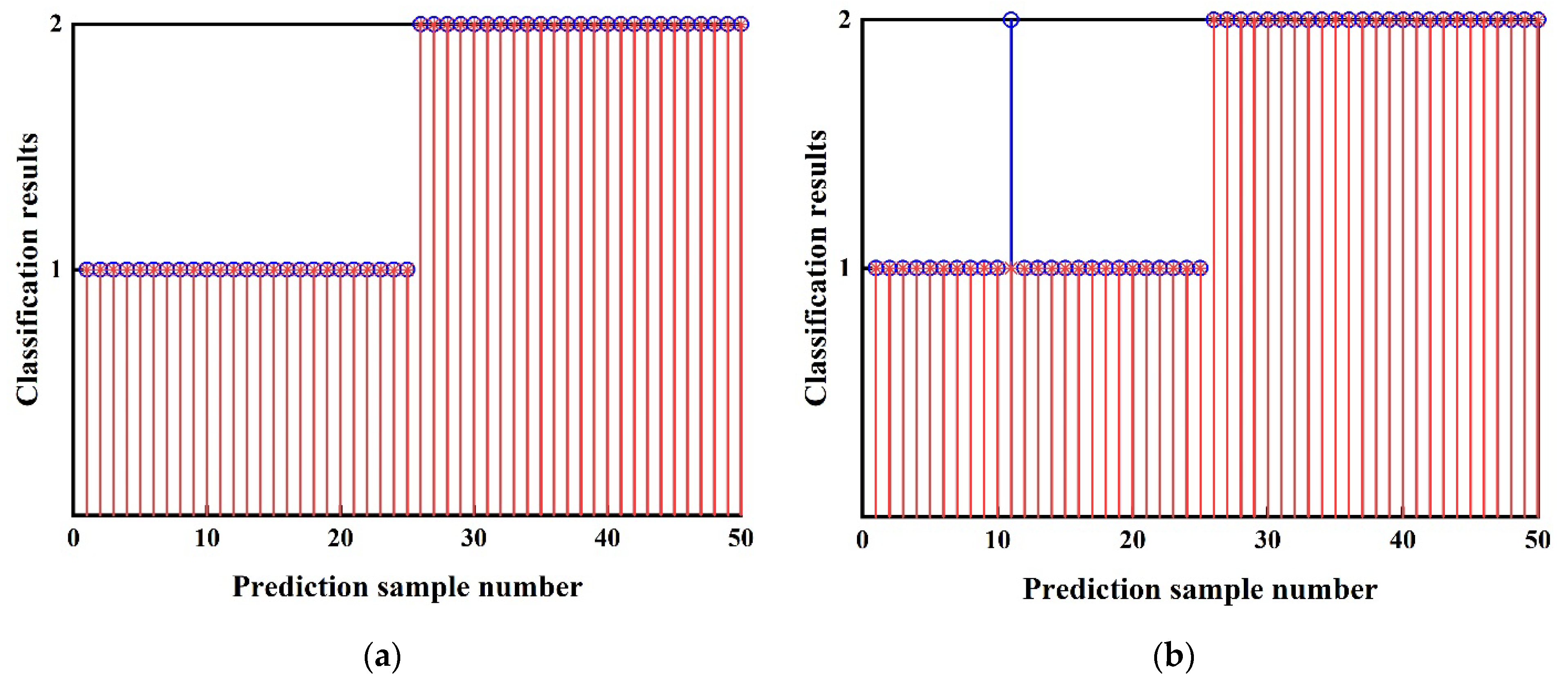
The recognition results of the feature vectors extracted based on ICEEMDAN are depicted in Figure 22. Figure 22a represents the recognition results without integrated noise signals, while Figure 22b illustrates the recognition results with integrated noise signals.

The analysis results above reveal that, without the inclusion of noise signals, the recognition results of the ICEEMDAN decomposition algorithm were all correct, achieving an accuracy of 100%. When the leakage signals were integrated with noise signals, the ICEEMDAN decomposition algorithm identified one leakage signal as a noise signal, with an accuracy of 98%. Therefore, it can be observed that the method combining ICEEMDAN decomposition with PNN not only exhibits strong resistance to interference but also demonstrates significantly better performance in distinguishing leakage from noise signals, compared to the previous three methods.

5. Conclusions

By employing a combination of laboratory pipeline model experiments and on-site tests on offshore platforms, this study explores a method for characterizing and identifying pipeline leakage signals based on acoustic emission. The research ingeniously blends collected leakage acoustic emission signals with on-site noise signals. Signal feature analysis and research are conducted on identified leakage and noise signals, with optimization of the results achieved using four algorithms: EMD, VMD, CEEMDAN, and ICEEMDAN. The findings indicate that the damage identification algorithm based on ICEEMDAN exhibits high precision and excellent identification performance in the extraction and recognition of pipeline leakage signal features. Comparative analysis of the results obtained from the mentioned algorithms leads to the following conclusions:

(1)

EMD fails to effectively identify leakage signals under low signal-to-noise ratios. Without the inclusion of noise, VMD algorithm misidentifies five leakage signals as noise signals, achieving an accuracy of 90%. When leakage signals are integrated with noise, VMD algorithm incorrectly identifies 15 leakage signals as noise signals, resulting in an accuracy of only 70%.

(2)

While VMD can effectively recognize both leakage and noise signals, its resistance to noise interference is relatively poor. Without the inclusion of noise signals, the VMD algorithm misidentifies four leakage signals as noise signals, with an accuracy of 92%. When leakage signals are integrated with noise, VMD algorithm incorrectly identifies seven leakage signals as noise signals, resulting in an accuracy of 86%.

(3)

Although CEEMDAN demonstrates higher recognition accuracy than EMD and VMD methods, it suffers from residual noise and pseudo modes. Without the inclusion of noise signals, the algorithm misidentifies two leakage signals as noise signals, with an accuracy of 96%. When leakage signals are integrated with noise, the algorithm incorrectly identifies three leakage signals as noise signals, achieving an accuracy of 94%.

(4)

In the case of ICEEMDAN, without the inclusion of noise signals, all recognition results are correct, with an accuracy of 100%. When leakage signals are integrated with noise, the algorithm incorrectly identifies one leakage signal as a noise signal, achieving an accuracy of 98%. This algorithm not only demonstrates high recognition accuracy but also addresses the issues of residual noise and pseudo modes. It is evident that the improved adaptive noise complete ensemble empirical mode decomposition method is effective in identifying both leakage and noise signals, exhibiting strong resistance to noise interference.