Changing Humboldt Squid Abundance and Distribution at Different Stages of Oceanic Mesoscale Eddies

Abstract

Humboldt squid, Dosidicus gigas, is one of the main economic cephalopod species off Peruvian waters, and their abundance and distribution are regulated by localized oceanic mesoscale dynamical processes. To this end, the present study employs normalization and frequency distribution methods, combining mesoscale eddy, oceanic environment, and D. gigas fishery data. This is the first exploration into the different stages of mesoscale eddies during their evolution off Peruvian waters and their influence on the regional marine environment, as well as the abundance and distribution of D. gigas resources. The results indicate that across the four stages of eddies, namely formation, intensification, mature, and aged, their kinetic energy and structure follow a pattern of “growth–equilibration–decay”. The abundance of D. gigas within the eddy’s covered zone undergoes an initial increase, followed by a decrease during the evolution of the four stages, peaking during the eddy’s mature stage. The abundance of D. gigas was higher in the anticyclonic eddies than that in the cyclonic eddies under different stages. The environmental factors conducive to D. gigas in eddies exhibited similar changes to D. gigas abundance throughout the eddy’s different stages. Our research emphasizes that anticyclonic eddies, during their evolution, exerted a more significant impact on the abundance and distribution of D. gigas in the Peruvian waters compared with cyclonic eddies. The eddy-induced changes in water temperature and productivity caused by the eddies may be the primary drivers of this impact.

1. Introduction

Mesoscale eddies are termed the “weather” of the ocean, characterized by the rotational flow of water. Their temporal scale spans from several weeks to months, while their spatial extent ranges from tens to hundreds of kilometers [1]. They are widely distributed across the oceans, accounting for approximately one-fourth of the Earth’s ocean surface [2]. In the Northern Hemisphere, mesoscale eddies, rotating both clockwise and counterclockwise, are referred to as anticyclonic eddies (AEs) and cyclonic eddies (CEs), respectively (the nomenclature is reversed in the Southern Hemisphere). Each eddy undergoes processes of generation, evolution, and dissipation, with its internal structure continuously changing throughout its cycle. Beyond their intrinsic rotational motion, eddies also propagate horizontally, covering several thousand kilometers from their formation to dissipation [3]. Eddies influence oceanic heat advection, ocean mixing, and water mass distribution in both horizontal and vertical dimensions [4], carrying substantial energy and playing a pivotal role in the transport of oceanic kinetic energy, heat, salinity, and carbon–silicate cycling [5].

In the 1980s, targeted research was carried out on the impacts of mesoscale eddies on a range of factors, from planktonic organisms to large marine life [6]. In marine ecosystems, phytoplankton are the predominant energy source for most marine organisms, playing a pivotal role as the primary producers and forming the foundation of the food web [7]. Mesoscale eddies influence phytoplankton through at least six mechanisms, including processes induced by the eddy’s rotation and horizontal movement, such as trapping, stirring, pumping, and mixing [6,8,9]. Early studies indicated that CEs corresponded to high-productivity regions [10], whereas AEs were associated with low-productivity zones [6]. Eddies primarily affect the distribution and abundance of marine pelagic predators in three ways [11]: (1) by serving as gathering points for prey and nutrients, thereby forming biological oases; (2) by providing pathways for survival or foraging through processes such as current transport, the entrainment of water masses, and the regulation of the vertical water column thermal structure; and (3) the protection and survival of eggs, larvae, and juveniles of marine pelagic predators. Marine organisms exhibit distinct responses to eddies, and even the same species may respond differently in different regions. For example, swordfish production in the northwest Atlantic is highest in eddy-free areas, while in the Kuroshio extensions in the northwest Pacific, swordfish production is positively correlated with warm eddies [7,12]. These variations may stem from differences in the ocean’s background environment, as well as habitat and behavioral disparities among different geographic populations [7].

The oceanic circulation structure in the Humboldt Current System (HCS) is notably intricate, comprising the Peruvian Coastal Current (PCC), the Peruvian Oceanic Current (POC), the Peru–Chile Counter Current (PCCC), and the Peru–Chile Undercurrent (PCUC), manifesting flow directions toward the south or north [13,14]. Influenced by alongshore equatorward winds and wind stress curl, deep cold water upwelling in Peruvian coastal waters brings nutrients from the deep sea to the surface [15]. Through phytoplankton photosynthesis, this process provides exceptional material conditions for the growth and development of fish in the region, creating renowned fishing grounds. The jumbo flying squid, Dosidicus gigas, represents a quintessential cephalopod catch in Peruvian fisheries, renowned for its abundance, ease of capture, and high economic value [16]. Consequently, it has become a primary target for fishing activities in countries including China, Japan, South Korea, Peru, and Chile [17,18]. The dietary composition of D. gigas does not differ with age, but the proportions vary. D. gigas preys on low trophic level organisms such as small- to medium-sized pelagic fish, crustaceans, and other cephalopods, while also serving as a significant food source for higher trophic level organisms, including large fish, marine mammals, and seabirds, making it a vital component of the marine food web [19,20,21,22]. As with other cephalopods, D. gigas generally do not live for more than 1 year [23].

Mesoscale eddies are widespread in the Peruvian Sea and are mostly generated in the southern coastal areas of Peru [24]. Under the influence of mesoscale eddies, local environmental conditions, including temperature, salinity, and current structures, undergo abrupt changes in this area [15,25]. As a species with a short lifecycle, D. gigas is highly sensitive to environmental fluctuations, rapidly adjusting its biological characteristics and distribution to adapt to new conditions [26,27]. Previous studies have shown that large-scale climate events such as El Niño, La Niña, and the Pacific Decadal Oscillation can alter the distribution and abundance of D. gigas [28,29]. However, research on how mesoscale eddies affect the distribution and abundance of D. gigas is scarce. Analyses of equatorial regions using the maximum entropy model have shown that D. gigas prefers to inhabit areas with relatively low eddy kinetic energy [30]. The eddy pumping induced by eddies provides abundant nutrients for D. gigas, creating high-quality habitats within the eddies [31].

Although these studies have explained, to some extent, the association between eddies and D. gigas resources, the question of how CEs and AEs differentially affect D. gigas during the evolution of the eddies remains unclear. Based on the above information, this study hypothesizes that variations in the abundance and spatial distribution of D. gigas are associated with eddy-driven environmental changes. Therefore, using mesoscale eddy, marine environment, and fishery catch data of D. gigas, this paper analyzes the spatial and temporal patterns and basic characteristics of eddies in Peruvian waters. It further determines the environmental changes induced by the two-eddy polarity in different stages, as well as their impacts on the abundance and spatial distribution of D. gigas using normalization and frequency distribution methods, focusing on exploring the differences in the impacts of these two types of eddies on D. gigas. These results will provide a basis for the sustainable management of fishery catches of this species.

2. Materials and Methods

2.1. Fisheries Data

This study utilized D. gigas fishing data provided by the China Distant-Water Fisheries Data Center at Shanghai Ocean University for the period from January to December 2019. The dataset comprises 45,435 records, and the research area spans from 75° to 95° W and 8° to 20° S. The data include operational details such as fishing locations (longitude and latitude), operational dates (year, month, day), detailed catch (unit: tons), fishing effort (operational days, unit: days), and catch per unit effort (CPUE, unit: tons/day). The calculation formula for CPUE is as follows:

$$\mathrm{CPUE}=\frac{\sum \mathrm{C}}{\sum \mathrm{E}}$$

where C denotes the catch in the fishing position, and E denotes the fishing effort in the fishing position.

2.2. Environmental Data

Merged data from multiple satellite altimeters were extensively utilized to identify and track mesoscale eddies. In this study, we used merged data from multiple satellite altimeters provided by the Copernicus Marine Environment Monitoring Service (CMEMS) (https://data.marine.copernicus.eu/product/SEALEVEL_GLO_PHY_L4_MY_008_047/download?dataset=cmems_obs-sl_glo_phy-ssh_my_allsat-l4-duacs-0.25deg_P1D_202112, accessed on 13 July 2023). This dataset includes absolute dynamic topography and sea surface velocity data, with a spatial resolution of 0.25° × 0.25° and a temporal resolution of 1 day.

Previous studies have indicated that variations in chlorophyll-a concentration (Chl-a), sea surface temperature (SST), and the temperature at the 50 m water layer (T_50m) were related to the spatial distribution and abundance of D. gigas [31,32,33]. Therefore, in this study, SST and T_50m were sourced from CMEMS’s Global Ocean Ensemble Reanalysis product (https://data.marine.copernicus.eu/product/GLOBAL_REANALYSIS_PHY_001_031/description, accessed on 13 July 2023) with a spatial resolution of 0.25° × 0.25° and a temporal resolution of 1 day. Chl-a data were obtained from CMEMS’s Global Ocean Satellite Observations product (https://data.marine.copernicus.eu/product/OCEANCOLOUR_GLO_BGC_L4_MY_009_104/download?dataset=cmems_obs-oc_glo_bgc-plankton_my_l4-gapfree-multi-4km_P1D_202207, accessed on 13 July 2023), with a spatial resolution of 4 km × 4 km and a temporal resolution of 1 day. All environmental data cover the required time and space range for the study and were matched with the fishing data using linear interpolation.

2.3. Mesoscale Eddy Analysis

This study employed the Angular Momentum Eddy Detection and Tracking Algorithm (AEDMA) for the identification and tracking of eddies [34]. This algorithm demonstrates robustness to grid resolution, accurately identifies merging and splitting events between eddies, and does not require the fine tuning of specific parameters, making it applicable to various velocity fields with different spatial resolutions. The AEDMA algorithm was used to generate a dataset containing various parameters of mesoscale eddies, such as their lifetime, radius, eddy center position, and velocity. The spatial distribution of the number of eddies and the catch of D. gigas in 2019 are shown in Figure 1. To characterize the propagation features of these eddies, the difference in eddy center positions between each day during an eddy’s lifetime and its first day were computed, based on the latitude and longitude information of the eddy center in the dataset. This approach aimed to obtain the relative trajectory of each eddy. Additionally, the eddy kinetic energy (EKE) was calculated using the following formula [35]:

$$\mathrm{EKE}=\frac{{U^{\prime }}_g^2+{V^{\prime }}_g^2}{2}$$

where ${U^{\prime }}_g$ and ${V^{\prime }}_g$ is the were the anomalies of zonal and meridional geostrophic currents.

2.4. Normalized Eddy Lifetime

Mesoscale eddies undergo continuous evolution throughout their cycle, resulting in dynamic impacts on marine life. To depict the evolving patterns of mesoscale eddy parameters and their influence on D. gigas throughout their cycle, a normalization process was applied to the eddy lifetime. Each individual eddy lifetime was segmented into four stages, defined as proportions of the total lifetime ranging from 0 to 1 [36]: the formation stage (0~0.1), intensification stage (0.1~0.3), mature stage (0.3~0.8), and aged stage (0.8~1). The normalized treatment was then applied to the radius, velocity, and EKE of all eddies within the study area. The averaged results yield the evolutionary curves of fundamental parameters characterizing mesoscale eddies.

2.5. The Relationship between Eddies and the Fishing Effort, Catch, and CPUE of D. gigas

To mitigate the influences of temporal and spatial factors (such as month, longitude, and latitude) as well as environmental factors (SST, T_50m, and Chl-a) on D. gigas CPUE, this study employed a random forest model for standardizing CPUE. Random forest (RF) emerges as a machine learning paradigm pioneered by Breiman [37], specifically tailored for regression scenarios. Renowned for its expeditiousness and adaptability, RF proves particularly adept at handling voluminous datasets laden with multidimensional features. The algorithm for RF in regression proceeds was as follows [38]: (1) Draw n_tree bootstrap samples from the original dataset. For each bootstrap sample, cultivate an unpruned regression tree. (2) At each node, randomly select m_try predictors and opt for the best split from among those variables. (3) Forecast new data by consolidating the predictions of the n_tree trees, typically through averaging for regression. In this study, the input factors of the RF were environmental and spatiotemporal factors (SST, T_50m, Chl-a, month, longitude, and latitude), and the output factor was CPUE. The parameter n_tree was set to 500, and the parameter m_try was set to 2.

To explore the impact of eddies on the abundance and distribution of D. gigas, an analysis of the spatial relationship between the eddies and the distribution of squid was conducted. Eddies can influence marine ecosystems within a range of twice their radius [39]. Consequently, the coverage area of eddies was expanded to twice their radius, including the eddy interior (EI) (0–R) and the eddy periphery (EP) (R–2R) [40]. First, an in-polygon algorithm was used to calculate whether the D. gigas fishing position was within the eddy influence range daily. When the D. gigas fishing position was within the influence range of more than one eddy, it was judged to be influenced by the eddy closest to the eddy center location. Second, because of the differences in eddy radius, the method of Zhang et al. [41] was used to calculate the normalized relative distances between the daily eddies’ centers and the D. gigas fishing position within their ranges. Finally, a grid of normalized radial distances from the eddy centers based on the radius of the eddy was created to represent the range of twice the radius of the eddy (±2R), defined by the radius of a circle covering the same area. For each eddy, each day on which it was detected could be represented by the grid and, based on the normalized relative distances from the daily eddies’ centers and D. gigas fishing locations in their ranges, the distribution pattern of catch, fishing effort, and CPUE of D. gigas within the range of influence of the eddies were determined. In addition, the normalized relative distances were then divided into 20 intervals of 0.1× radius intervals from the inside to the outside, and the total fishing effort, total catch, and CPUE of D. gigas within each interval were calculated. Furthermore, to compare the disparities in fishing effort, catch, and CPUE between the EI and EP, a t-test analysis was conducted. The eddy containing the fishing position was divided into stages according to the time of operation and its lifetime, and then the change in D. gigas within the eddy in each life stage was analyzed according to the above method. To better represent the changes in D. gigas within the eddies, only the status of the eddies on the day when there were fishing position within the eddies were counted.

The generalized additive model (GAM) is adept at capturing nonlinear relationships between the response variable and multiple predictor variables [42]. In this study, the GAM model was employed to analyze the statistical relationship between the abundance of squid CPUE and eddy parameters. Specifically, the squid CPUE was regarded as the response variable, while the variables of AE (CE) radius, AE (CE) velocity, and distance from the center of AE (CE) were considered as predictors. To address multicollinearity among variables, the variance inflation factor (VIF) was utilized for examination [43]. The GAM model utilized the natural logarithm as the link function and added a constant of 0.1 to the CPUE values to prevent zero values. Hence, the GAM model expression was as follows:

$$\ln \left(\mathrm{C}\mathrm{P}\mathrm{U}\mathrm{E}+0.1\right)=s\left(\mathrm{r}\mathrm{a}\mathrm{d}\mathrm{i}\mathrm{u}\mathrm{s}\right)+s\left(\mathrm{v}\mathrm{e}\mathrm{l}\mathrm{o}\mathrm{c}\mathrm{i}\mathrm{t}\mathrm{y}\right)+s\left(\mathrm{d}\mathrm{i}\mathrm{s}\mathrm{t}\mathrm{a}\mathrm{n}\mathrm{c}\mathrm{e}\right)+\epsilon$$

Here, s denoted the smooth spline, where radius and velocity denoted radius and rotating speed of the fishing position from the nearest AE or CE, respectively, and distance indicated the relative distance of the fishing position from the nearest AE or CE center. ε denoted the random error.

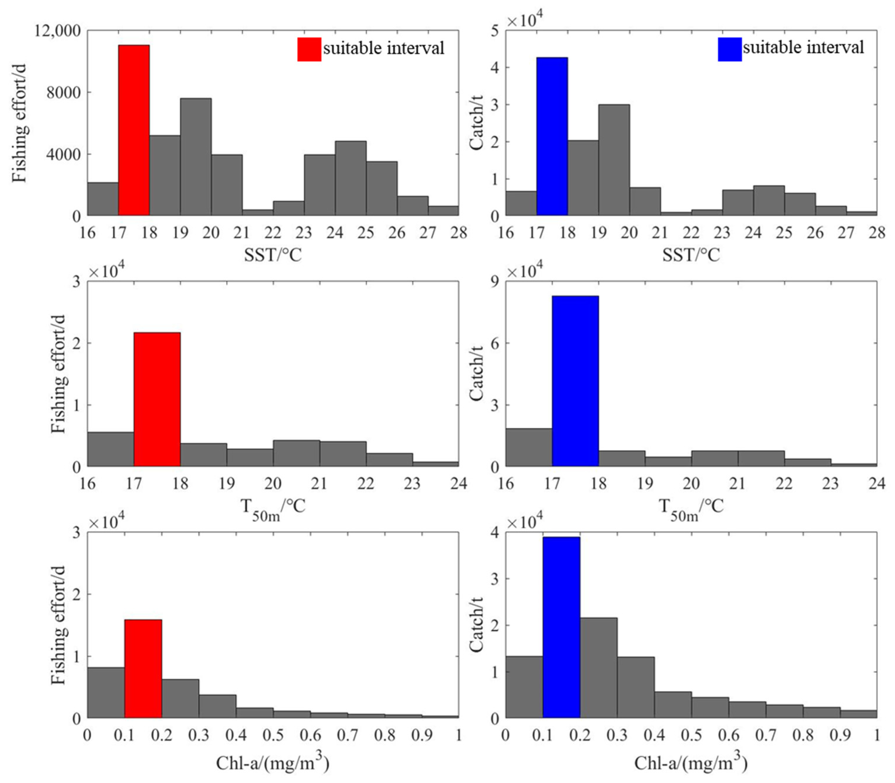
2.6. Changes in Suitable Environments for D. gigas in Eddies

Based on the frequency distribution method, each environmental factor was divided into different intervals, and the sizes of fishing effort and catch within different intervals were counted. From this, the suitable environmental distribution range of D. gigas was calculated, and the range in which the highest fishing effort and catch were distributed was defined as the optimal environmental range of D. gigas.

To analyze the changes in the distribution of suitable environmental factors within eddies at different life stages, a normalized grid of radial distances from the eddy centers based on the radius of eddies was established, as described in Section 2.5. Then, the marine factor variables were interpolated into the grid of each eddy, and the sum of the number of occurrences of the environmental data inside and outside each eddy was calculated based on the different intervals. To better represent the changes in the suitable environment for D. gigas within the eddies, only eddy status on the day when there were fishing position within the eddy were counted.

3. Results

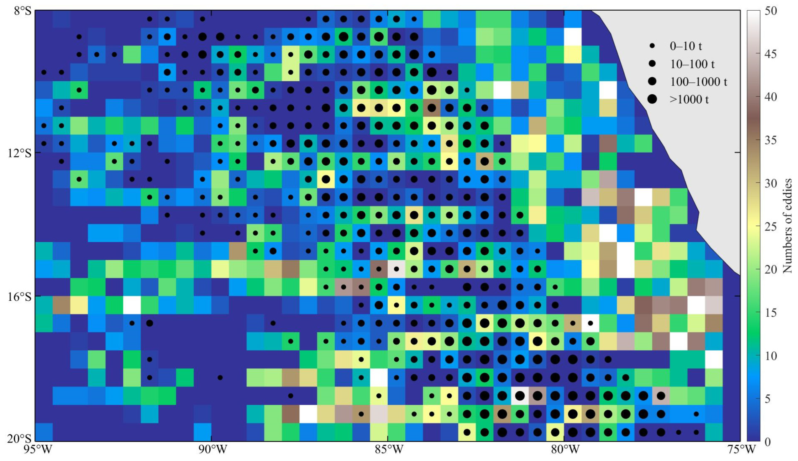
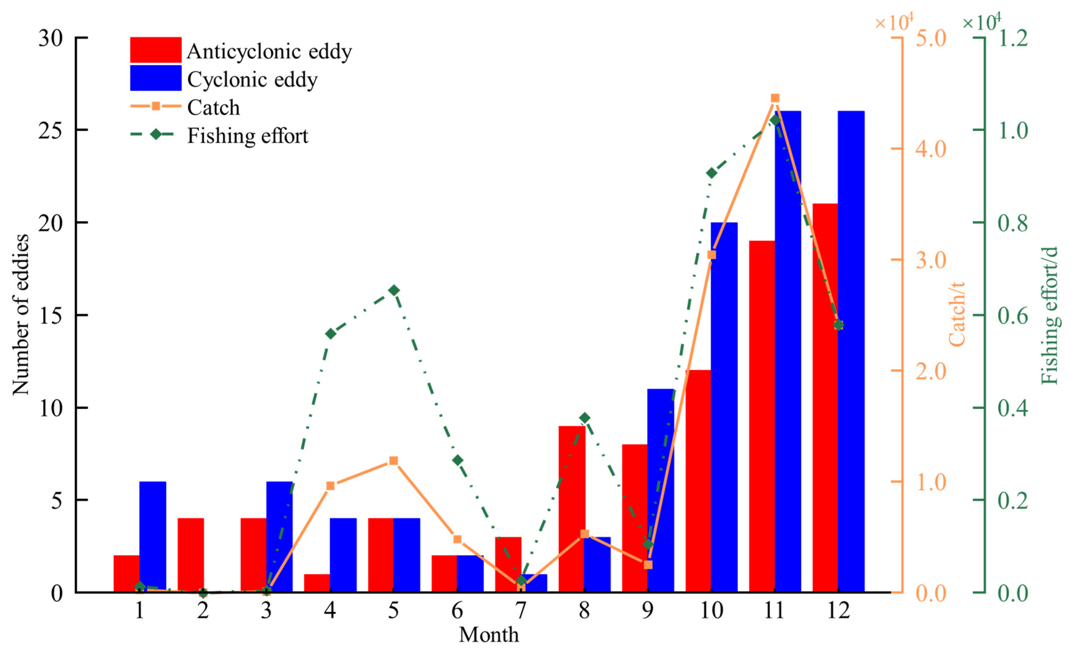
3.1. Monthly Variation in the Number of Eddies, D. gigas Catch, and Fishing Effort

Mesoscale eddies were identified and tracked from January to December 2019 within the D. gigas fishery (8° to 20° S, 75° to 95° W) in Peruvian waters based on the AEDMA method. Using the Lagrangian method (which considers the entire lifetime of an eddy as one eddy), 198 eddies were counted, with less AEs than CEs (89 and 109, respectively), both with similar trends. As a whole, the number of eddies was low in January–August and showed a significant increasing trend in September–December, with the highest number of eddies in December (45) (Figure 2). The total fishing effort and total catch of D. gigas in January–December were 4.54 × 10⁴ d and 13.42 × 10⁴ t, respectively, and fishing effort was higher in April–May and October–December, with a maximum value of 1.02 × 10⁴ days. The catch was smaller in January–September, not exceeding 1.2 × 10⁴ t, and higher in October–December, with a maximum value of 4.46 × 10⁴ t. There was a tendency for the catch and fishing effort to increase in parallel with the number of eddies in September–November. The t-test showed that the difference in fishing effort and catch of D. gigas between January–September and October–December was highly significant (p < 0.001).

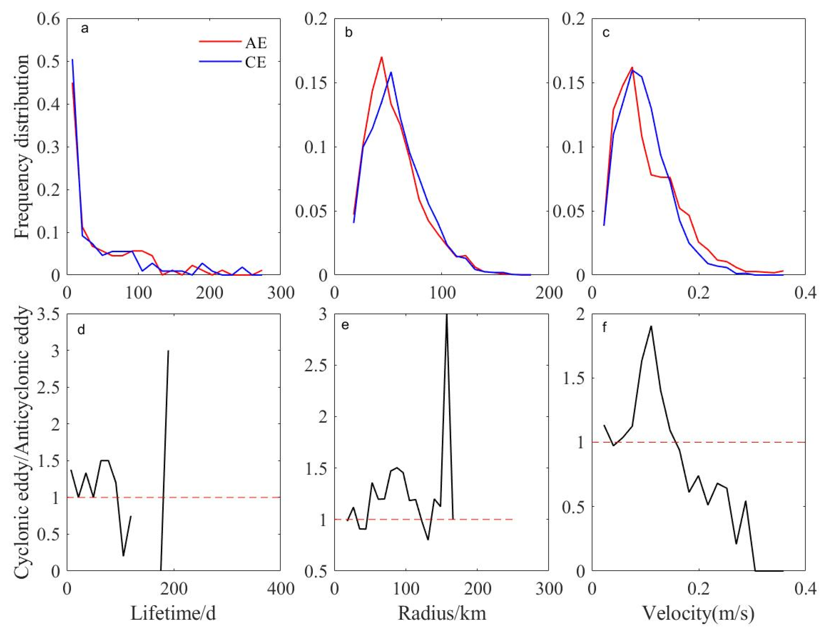
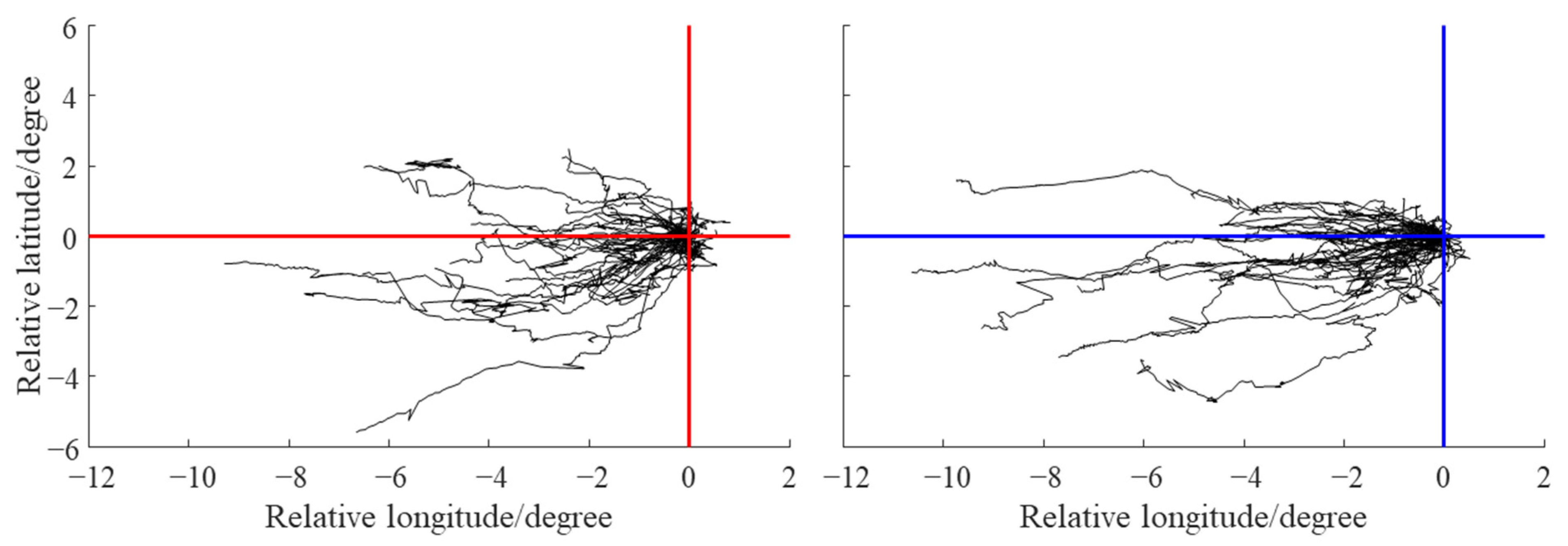
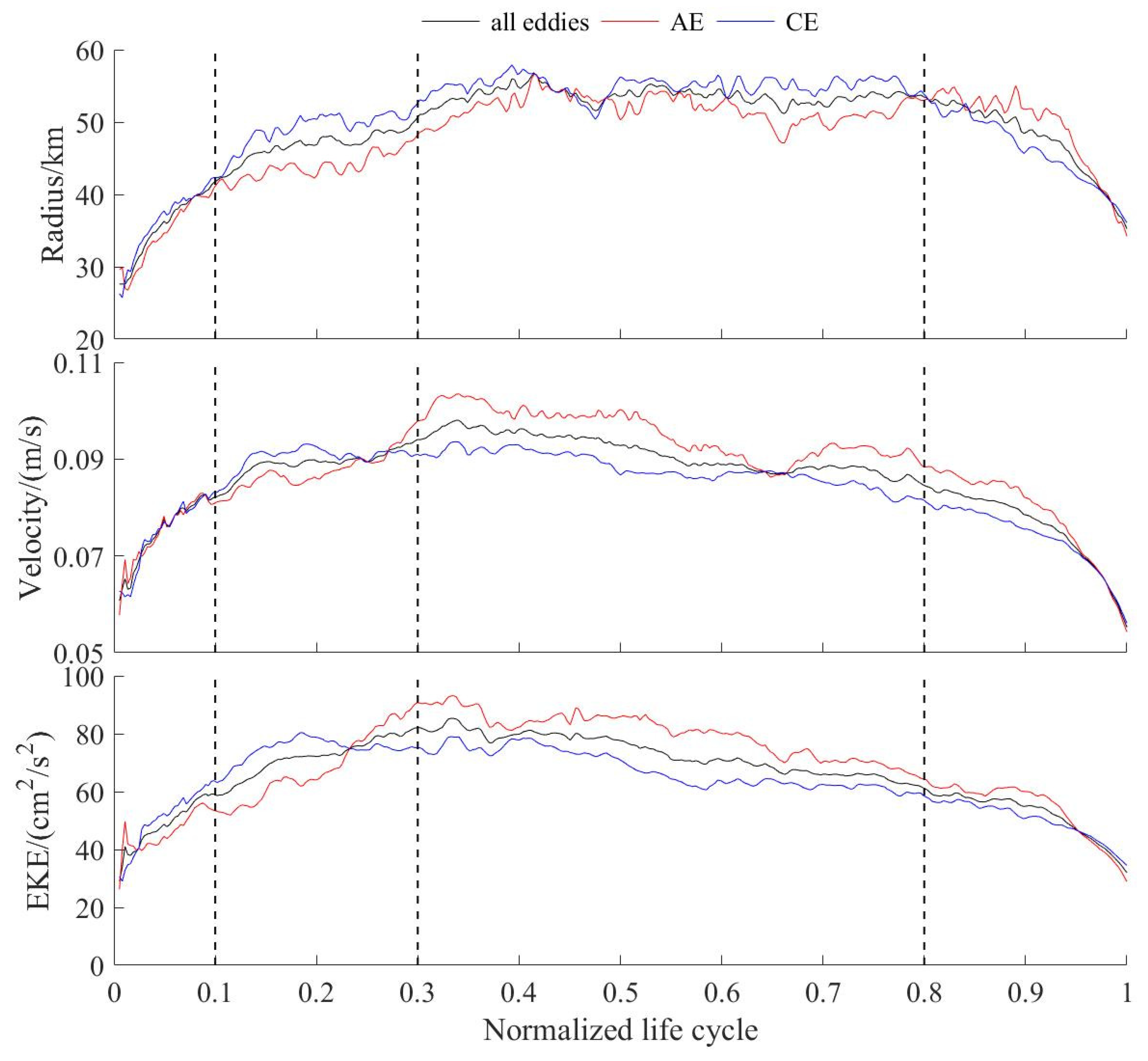
3.2. Characteristic Parameters and Trajectories of Eddies

Figure 3a shows a sharp decrease in the number of eddies with the increase in their lifetime, with the majority having a lifetime of less than 100 days. CEs have an average lifetime of 42.38 days, while AEs have an average lifetime of 45.40 days. Among eddies with a lifetime less than 94 days, CEs have a slightly higher prevalence, whereas for eddies with a lifetime exceeding 94 days, AEs dominate (Figure 3d). The frequency distribution of the eddy radius is generally consistent (Figure 3b), with the peak located around 50 km. The average radius for CEs and AEs are 58.31 km and 55.76 km, respectively. In most radius ranges, CEs are more abundant (Figure 3e). The frequency of velocity for CEs and AEs follows a skewed distribution, with AEs exhibiting a slightly higher average velocity (0.10 m/s) compared with CEs (0.09 m/s) (Figure 3c). For eddies with a velocity exceeding 0.16 m/s, AEs predominate (Figure 3f).

The study analyzed the propagation characteristics of eddies off Peruvian waters. The origin point (0°, 0°) was designated as the generation location for eddies, and their relative propagation features concerning longitude and latitude are depicted in Figure 4. In the east–west direction, both CEs and AEs exhibit distinct westward propagation tendencies (78% of CEs and 80% of AEs). In the north–south direction, the majority of eddies move southward (47% of CEs and 39% of AEs). The maximum westward propagation distance for AEs is approximately 9.1°, and the southward propagation is about 5.5°. For CEs, the maximum westward propagation distance is around 10.6°, with a southward propagation of approximately 3.4°.

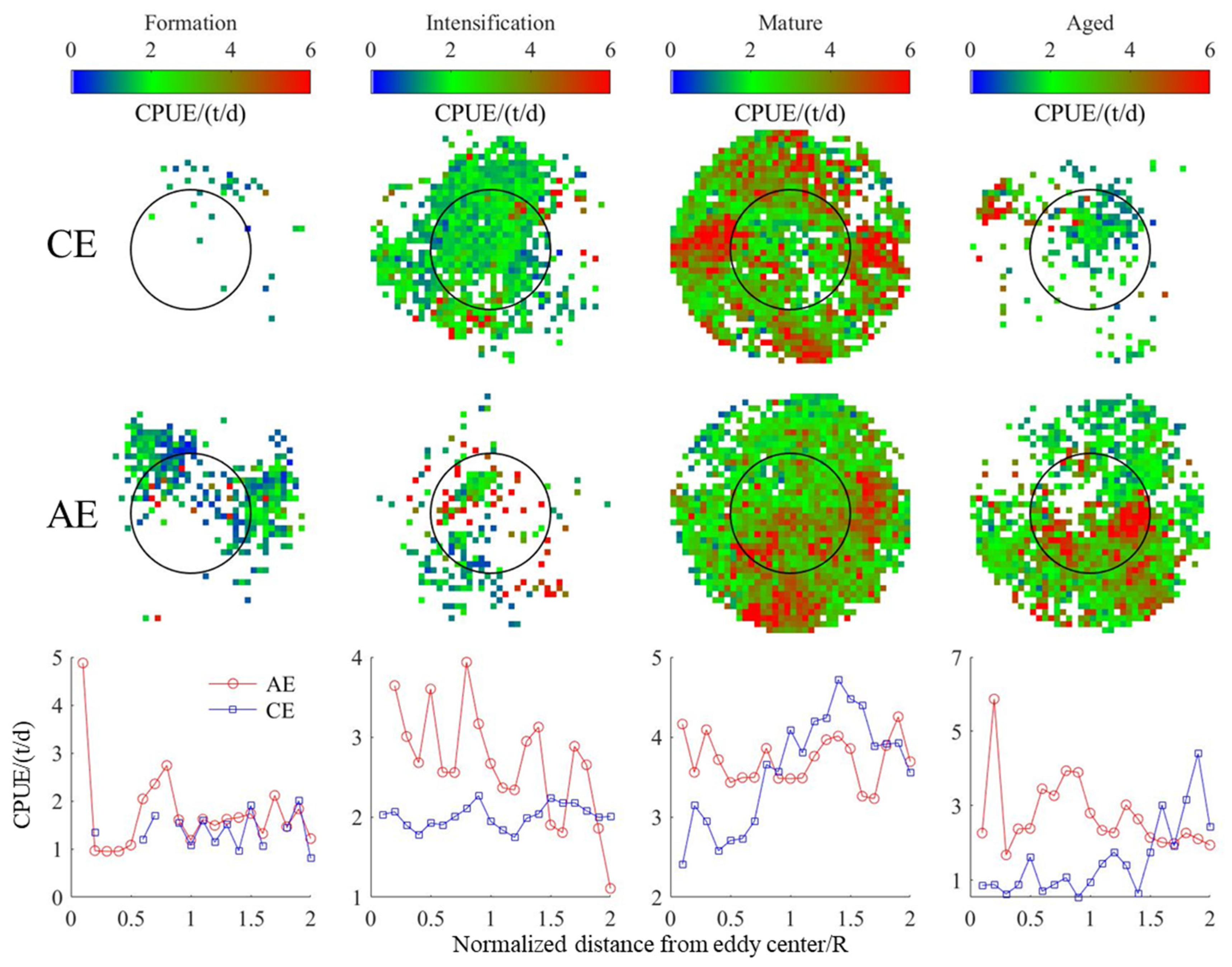
3.3. Changes in Eddies Characteristics over Different Stages

Figure 5 illustrates the variation curves of velocity, radius, and EKE of eddies over different life stages off Peruvian waters. The evolution trends of CEs, AEs, and all eddies off Peruvian waters are basically the same, with an overall increasing and then decreasing trend. The radius, velocity, and EKE of CEs (AEs) reached their maximum at 0.39 (0.41), 0.34 (0.34), and 0.18 (0.33), respectively. Throughout most of the time, CEs exhibited larger radius compared to AEs, while the velocity and EKE of CEs tended to be smaller than those of AEs.

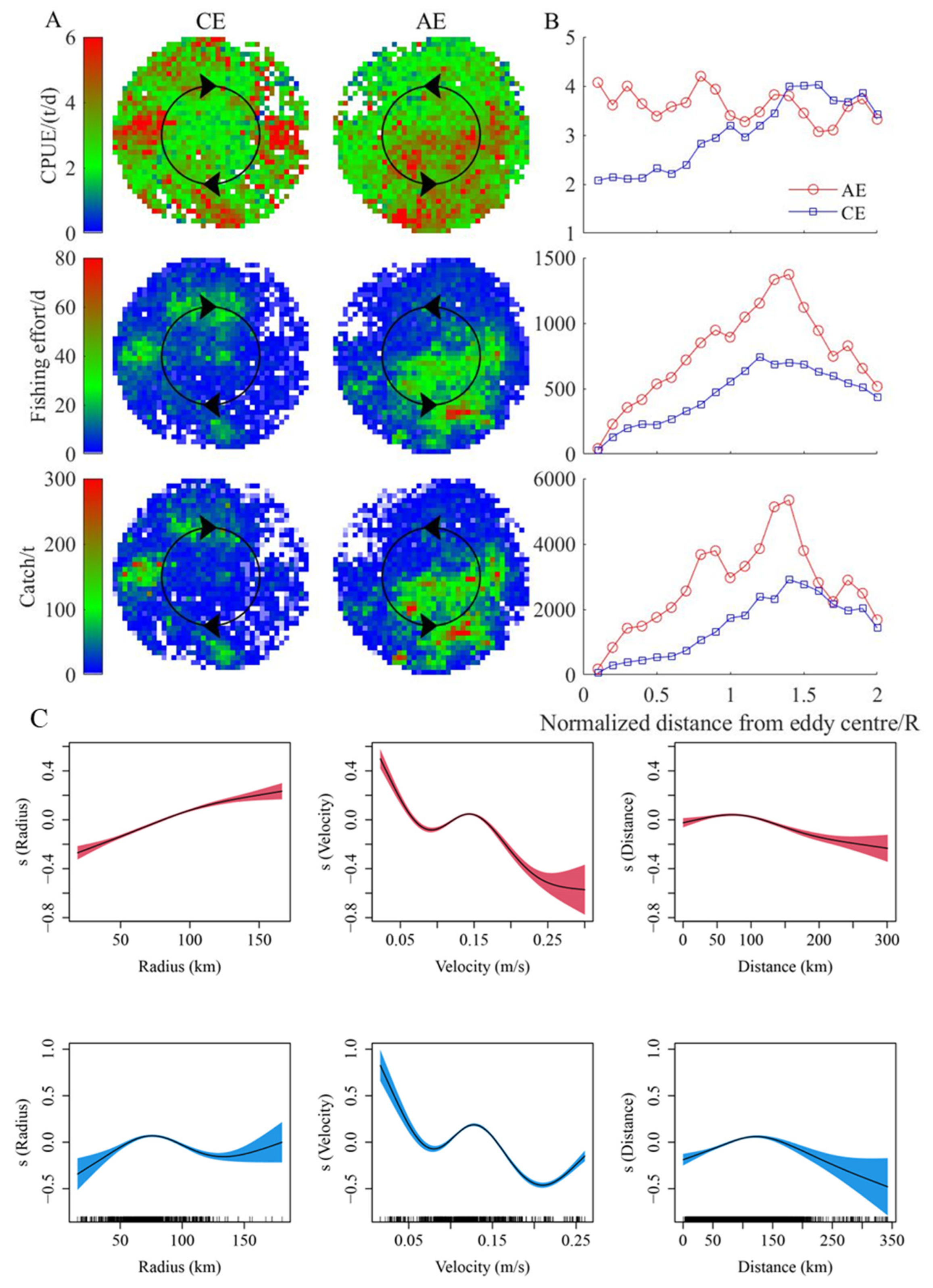
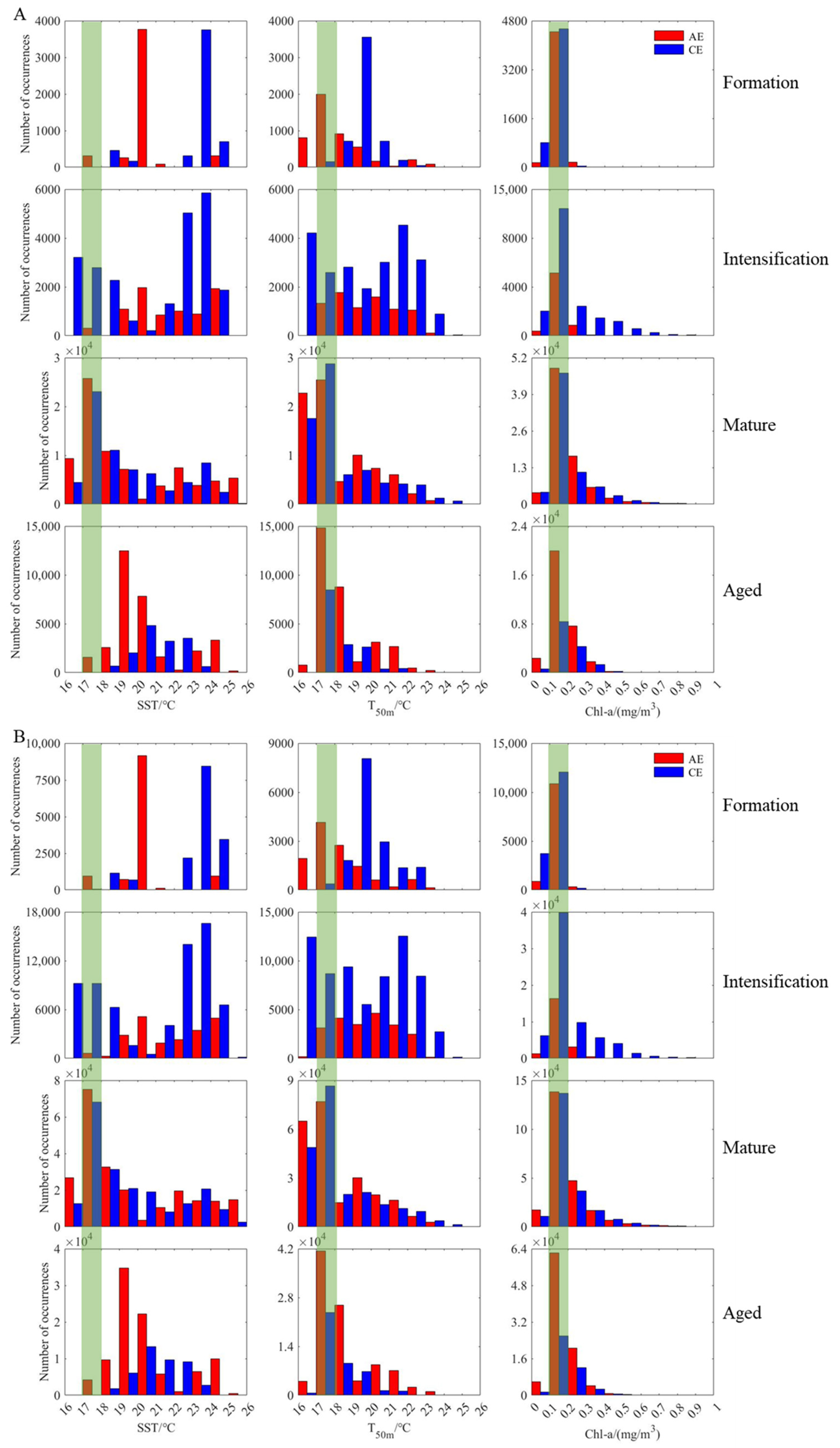
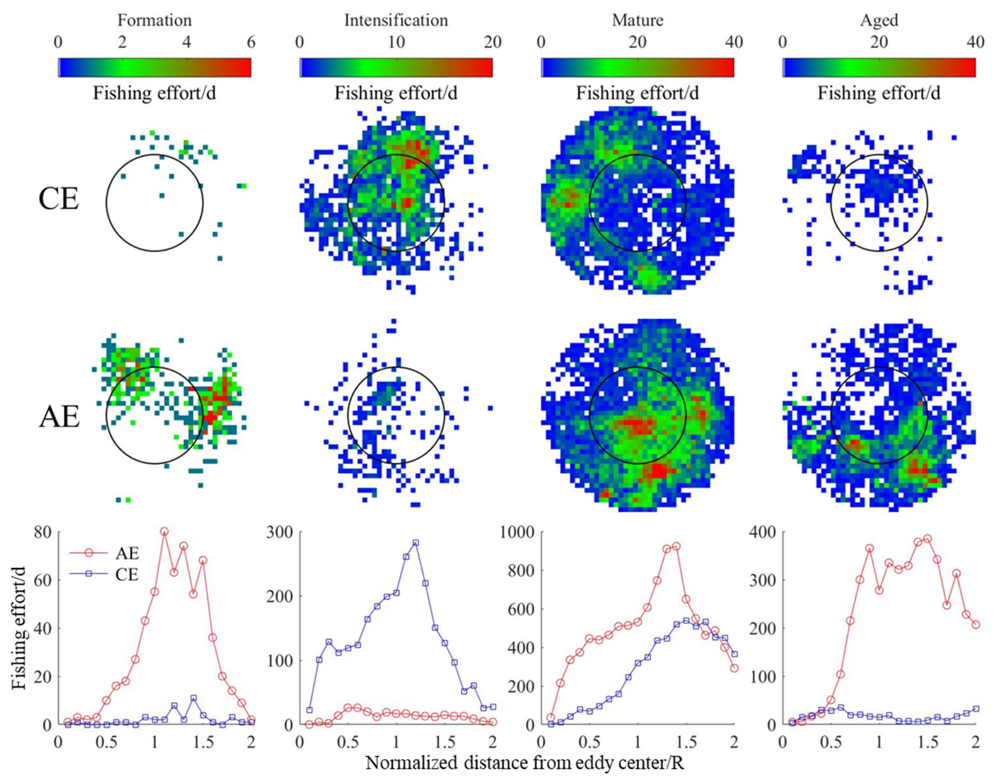
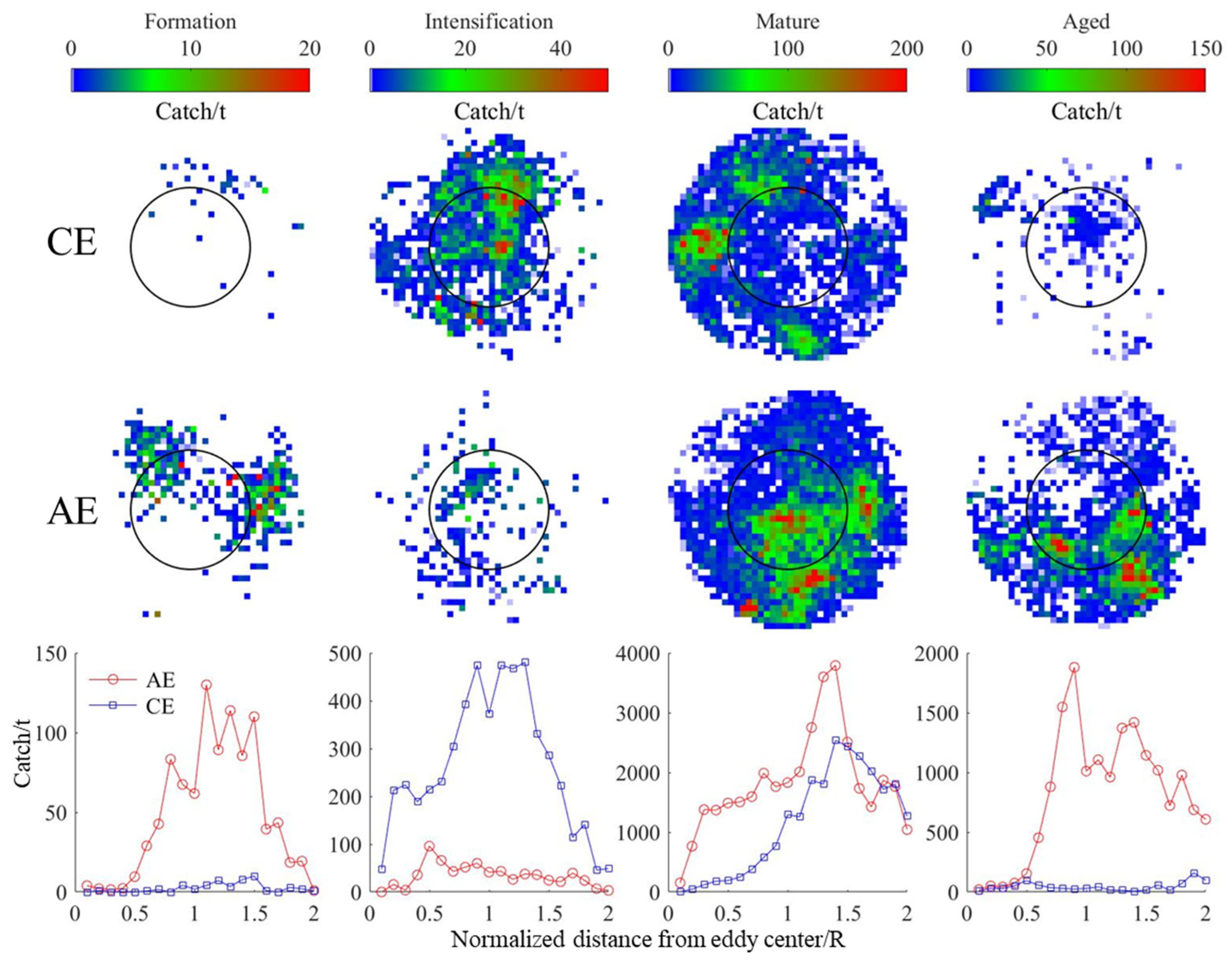
3.4. Changes in D. gigas and Suitable Environments during Different Eddy Stages

Figure 6A illustrates the spatial distribution of D. gigas within the 2× radius range of CEs and AEs. Elevated CPUE values for D. gigas were predominantly observed in the peripheral regions of CEs, while both the interior and periphery of AEs exhibit high values. In terms of fishing effort, the fishing effort within CEs is relatively low and dispersed, whereas the fishing effort within AEs is comparatively higher and concentrated on the southeast side of the eddy center. Regarding the catch, regions with high squid catch volumes are concentrated in the periphery of eddies, reaching a maximum of 272.9 t. Notably, higher D. gigas catch volumes are also observed both interior and peripheral to the southeastern side of the AEs center, with a maximum of 550.55 t.

The variations in CPUE, fishing effort, and catch for D. gigas within the 2× radius of AEs and CEs are depicted in Figure 6B. It is evident that with increasing distance from the AEs center, D. gigas CPUE decreases. Conversely, with increasing distance from the CEs center, the D. gigas CPUE showed an initial increase followed by a decrease. The CPUE in the interior region of the AEs was noticeably higher than in the interior region of the CEs. Specifically, the average D. gigas CPUE in the interior region of the AEs was 3.74 t/d, while in the interior region of the CEs, it was 2.43 t/d. As the distance from the eddy center increases, the D. gigas catch and fishing effort within both types of eddies show the same trend, characterized by an initial increase followed by a decrease. Notably, values within the AEs are significantly higher than those within the CEs. Specifically, the D. gigas fishing effort and catch reach their maximum at a distance of 1.4 R from the AEs center, with values of 1373 d and 5.34 × 10³ t, respectively. The D. gigas fishing effort reaches its maximum at a distance of 1.2 R from the CEs center, with a value of 743 d, while the catch reaches its maximum at a distance of 1.4 R from the CEs center, with a value of 2.91 × 10³ t. The t-tests showed that the differences in CPUE, fishing effort, and catch between the interior and peripheral regions of the CEs and AEs were all significant (p < 0.05).

Based on the GAM model, the relationship between the abundance of D. gigas and the characteristic parameters of mesoscale eddies was analyzed (Figure 6C). Results from the model’s significance tests revealed that all variables exhibit highly significant correlations (p < 0.001). The radius of mesoscale eddies significantly impacted the CPUE of D. gigas. For AEs, CPUE demonstrated a positive correlation with radius, indicating an increase in D. gigas CPUE with larger radius. Conversely, within CEs, D. gigas CPUE initially increased and then decreased with increasing radius. The relationship between velocity and CPUE was consistent for both AEs and CEs, showing a pattern of decrease, followed by a slight increase, and then a decrease again as velocity increased. Additionally, a negative correlation existed between the distance from fishing position around the AEs and CEs center, indicating that D. gigas CPUE decreased as the distance from the eddy center increased.

Figure 7 shows the distribution of D. gigas CPUE within the 2× radius of eddies at different stages. The CPUE within the interior regions of AEs is consistently higher than that within CEs during all stages. In the formation, intensification, and dissipation stages, the CPUE in the peripheral regions of AEs is slightly higher than that in the peripheral regions of CEs. However, during the maturation stage, the CPUE in the peripheral regions of AEs is lower than that in the peripheral regions of CEs. As the eddies evolve, both types show an increasing and then decreasing trend in CPUE within both the interior and peripheral regions. The t-tests showed that the differences in CPUE between the interior and peripheral regions of the CE and AE over different stages were significant (p < 0.05).

The distribution of D. gigas fishing effort and catch within the 2× radius of eddies at different stages are shown in Figure 8 and Figure 9. Their trends are mainly characterized by an initial increase followed by a decrease, reaching their peak during the mature stage of eddy evolution. Except for the intensification stage, the D. gigas catch and fishing effort are higher in the interior and peripheral regions of the AE than in the same regions of the CE throughout the lifetime. Overall, both the catch and fishing effort of CE and AE show an increasing and then decreasing trend with an increasing distance from the eddy center. The t-tests showed that the differences in fishing effort and catch between the interior and peripheral regions of the CE and AE over different stages were significant (p < 0.05).

Figure 10 shows the fishing effort and catch within different intervals of environmental factors. Fishing effort and catch are predominantly concentrated within the SST range of 17–21 °C, with the optimal range being 17–18 °C. The T_50m range where fishing effort and catch are most concentrated is also 17–18 °C, accounting for approximately 50% of their respective totals. The range of Chl-a in which fishing effort and catch are mainly concentrated is 0.1–0.3 mg/m³, with an optimal range of 0.1–0.2 mg/m³.

Figure 11 illustrates the variation in the occurrence frequency of different environmental factors within the 2× radius range of the eddies throughout their lifetime. The changes in the occurrence frequency of the most suitable environmental factors are primarily characterized by an initial increase followed by a decrease over the eddy’s lifetime, reaching the highest frequency during the mature stage. The range of most suitable environmental conditions within 0–R for both CEs and AEs are notably lower than that in the outer R–2R range. Except for the intensification stage, the most suitable environmental factors in the interior of AEs have consistently higher values than those in the interior of CEs across different stages.

4. Discussion

4.1. Evolution and Spatial and Temporal Distribution Characteristics of Eddies off Peruvian Waters

The genesis of eddies off Peruvian waters is notably intricate. The interaction between the ocean current system and the coastline, the presence of strong upwelling fronts, and the high spatiotemporal variability of coastal currents could all contribute to the formation of coastal eddies in this area [24]. Utilizing Argo float data, the three-dimensional structure of mesoscale eddies in the southeastern Pacific Ocean has been constructed, identifying that CE within the intrathermocline are influenced by equatorial coastal currents, while subthermocline AEs may result from the detachment of the PCUC [25]. The results of this study indicate variations in the monthly distribution of eddy numbers in the Peruvian waters, with the majority forming between September and December. In 2019, CEs outnumbered AEs, and most eddies exhibited a pronounced westward propagation. These findings differ somewhat from those of other studies, possibly due to different counting methods and the lack of eddy data screening [44,45]. There are also notable differences in the parameter characteristics of CEs and AEs: the average lifetime of eddies is 43.74 days, with CEs and AEs having average lifetimes of 42.38 days and 45.40 days, respectively, showing little difference in their duration. This aligns more closely with previous studies [24]. The average radius of AEs is smaller than that of CEs, but their average velocity is slightly higher. Velocity generally reflects the intensity of eddies, indicating that AEs are stronger and have a longer duration. The evolution of eddies is a complex nonlinear event, generally following a simple grow–equilibrate–decay pattern. Additionally, for the convenient comparison of the characteristics of eddies with different lifetimes, some researchers have proposed various normalization methods based on the evolutionary pattern of eddies [36,46]. The results of this study suggest that the evolution curve of eddies in the Peruvian waters generally conforms to the aforementioned grow–equilibrate–decay pattern but is asymmetric. This deviation from global results on oceanic eddies may be influenced by the regional marine environment [47]. In the evolution process in the Peruvian waters, the EKE consistently remains below 100 cm²/s², lower than the EKE in other oceanic regions [24]. Overall, different types of eddies exhibit differences in variables such as radius, velocity, and EKE, which could potentially have varied impacts on the abundance and distribution of D. gigas.

4.2. Correlation Analysis of Eddies and D. gigas Distribution

CPUE refers to the average catch per unit of fishing effort in a specific fishing ground over a certain period. It is considered proportional to the abundance of fishery resources and is one of the most frequently used indicators of resource abundance [48,49]. However, it can sometimes be challenging to establish the proportional relationship between CPUE and resource abundance due to the influence of environmental effects, habitat area, and fisherman behavior, among others [50,51]. Some studies suggest that, under certain conditions, fishing effort may more accurately characterize fish abundance than CPUE [52,53]. Therefore, to reflect the relationship between D. gigas resources and eddies more precisely, this study employs three indicators: CPUE, fishing effort, and catch.

In April and May, there were fewer eddies in the offshore waters of Peru, and despite substantial fishing effort, the catch is relatively low. In contrast, from October to December, when the number of eddies increases, more fishing effort is exerted, resulting in a higher catch of D. gigas. It is evident that there is a certain relationship between the abundance of D. gigas and the number of eddies in the offshore waters of Peru. Furthermore, the results of this study indicate that D. gigas resource abundance is higher in AEs than in CEs in the offshore waters of Peru. Specifically, the resource abundance of D. gigas in the interior regions of AEs is higher than that in the interior regions of CEs, while there is no significant difference in the peripheral regions of the two types of eddies. CEs and AEs have different mechanisms of influence on the local marine environment, leading to distinct biological responses to these eddies. Previous studies have shown that high trophic level organisms such as northwest Atlantic bluefin tuna [12], southwest Atlantic loggerhead turtles [40], and north Atlantic blue sharks [54] are more likely to occur in AEs, while Northwest Atlantic yellowfin tuna [12], Northwest Pacific loggerhead turtles [55], and whale species in the Gulf of Mexico [56] are more likely to be found in CEs. Cephalopods may prefer the interior of AEs over CEs. For instance, during the unstable years of the northwest Pacific Kuroshio, the interior of AEs provides more suitable seawater temperatures and feeding conditions for D. gigas [41]. With increasing distance from the eddy center, the abundance of D. gigas shows different trends within the two types of eddies, similar to findings from a study of subtropical high trophic level fish species in the north Pacific [11].

Over the evolution of eddies, their kinetic energy and impacts on the marine environment should increase and then decrease. During the intensification stage of AEs, the fishing effort and catch of D. gigas are lower than that during their formation stage. However, the D. gigas CPUE during the intensification stage is higher than during the formation stage. Despite lower fishing effort and catch, the CPUE is higher. Therefore, we argue that the abundance of D. gigas in AEs is higher during the intensification stage compared with the formation stage. Comparing CPUE, fishing effort, and catch of D. gigas during different stages of the eddy’s lifetime reveals a consistent pattern of increasing and then decreasing D. gigas resource abundance within the influence range of the eddies. This pattern aligns with the changes in eddy characteristics.

4.3. Effects of Eddies on Seawater Temperature and Chlorophyll Concentration

Off Peruvian waters, in addition to affecting Chl-a vertically, eddies also transport nearshore waters rich in high Chl-a horizontally into the open ocean through their own westward propagation [57]. They also change the horizontal distribution and vertical structure of water temperature in the Peruvian waters by transporting water masses in their motion [15,25]. Therefore, the eddy contributes to drastic changes in temperature and Chl-a in its area of influence, which is also shown in this study. The optimal SST, Temp_50m, and Chl-a intervals for D. gigas in 2019 were 17–18 °C, 17–18 °C, and 0.1–0.2 mg/m³, respectively. The frequency of suitable environmental factors for D. gigas in the interior and peripheral regions during the evolution of the CEs and AEs first increased and then decreased, which is in line with the change in the abundance of D. gigas in their interior and peripheral regions. However, the frequency of suitable environmental factors for D. gigas in the interior and peripheral regions of the AEs was lower during the intensification stage. This is because only eddies with fishing position on the same day were selected in this study, and the number of AEs in this stage was relatively small. Comparing the frequency of suitable environmental factors in the interior and peripheral regions of the two types of eddies showed that there were more suitable SSTs and T_50m in the AEs in the formation stage of the eddies than in the CEs, that the number of suitable SST and Chl-a in the mature stage of the AEs was more than that of CEs, and that the ranges of the three kinds of suitable environmental factors in the AEs were more than that of CEs in the aged stage. The higher abundance of D. gigas inside the AEs in the formation, mature, and aged stages than that in the CEs may be caused by the distribution of eddy-influenced environmental factors.

5. Conclusions

Our research indicates that with the evolution of eddies (formation–intensification–mature–aged), the abundance of D. gigas within its influence zone initially increases and then decreases, reaching its peak during the mature stage of the eddy. Additionally, it underscores that AEs exert a more pronounced influence on the abundance and distribution of D. gigas off Peruvian waters during the evolutionary process compared with CEs. We infer that eddy-induced changes in water temperature and productivity are likely the primary factors for this impact. This study substantiates the significant influence of mesoscale dynamic processes on the distribution of cephalopod habitats and abundance fluctuations, elucidating the response of D. gigas stocks to eddy evolution. This provides a novel perspective for cephalopod resource management and sustainable fishing.

References

1. Chelton, D.B.; Schlax, M.G.; Samelson, R.M.; De Szoeke, R.A. Global Observations of Large Oceanic Eddies. Geophys. Res. Lett. 2007, 34, 2007GL030812. [Google Scholar] [CrossRef]
2. Xing, Q.; Yu, H.; Wang, H.; Ito, S.; Chai, F. Mesoscale Eddies Modulate the Dynamics of Human Fishing Activities in the Global Midlatitude Ocean. Fish Fish. 2023, 24, 527–543. [Google Scholar] [CrossRef]
3. Janout, M.A.; Weingartner, T.J.; Okkonen, S.R.; Whitledge, T.E.; Musgrave, D.L. Some Characteristics of Yakutat Eddies Propagating along the Continental Slope of the Northern Gulf of Alaska. Deep. Sea Res. Part II Top. Stud. Oceanogr. 2009, 56, 2444–2459. [Google Scholar] [CrossRef]
4. Lévy, M.; Klein, P.; Treguier, A.-M. Impact of Sub-Mesoscale Physics on Production and Subduction of Phytoplankton in an Oligotrophic Regime. J. Mar. Res. 2001, 59, 535–565. [Google Scholar] [CrossRef]
5. Zhou, K.; Dai, M.; Xiu, P.; Wang, L.; Hu, J.; Benitez-Nelson, C.R. Transient Enhancement and Decoupling of Carbon and Opal Export in Cyclonic Eddies. JGR Ocean. 2020, 125, e2020JC016372. [Google Scholar] [CrossRef]
6. McGillicuddy, D.J. Mechanisms of Physical-Biological-Biogeochemical Interaction at the Oceanic Mesoscale. Annu. Rev. Mar. Sci. 2016, 8, 125–159. [Google Scholar] [CrossRef]
7. Durán Gómez, G.S.; Nagai, T.; Yokawa, K. Mesoscale Warm-Core Eddies Drive Interannual Modulations of Swordfish Catch in the Kuroshio Extension System. Front. Mar. Sci. 2020, 7, 680. [Google Scholar] [CrossRef]
8. Godø, O.R.; Samuelsen, A.; Macaulay, G.J.; Patel, R.; Hjøllo, S.S.; Horne, J.; Kaartvedt, S.; Johannessen, J.A. Mesoscale Eddies Are Oases for Higher Trophic Marine Life. PLoS ONE 2012, 7, e30161. [Google Scholar] [CrossRef] [PubMed]
9. Chelton, D.B.; Gaube, P.; Schlax, M.G.; Early, J.J.; Samelson, R.M. The Influence of Nonlinear Mesoscale Eddies on Near-Surface Oceanic Chlorophyll. Science 2011, 334, 328–332. [Google Scholar] [CrossRef]
10. Falkowski, P.G.; Ziemann, D.; Kolber, Z.; Bienfang, P.K. Role of Eddy Pumping in Enhancing Primary Production in the Ocean. Nature 1991, 352, 55–58. [Google Scholar] [CrossRef]
11. Arostegui, M.C.; Gaube, P.; Woodworth-Jefcoats, P.A.; Kobayashi, D.R.; Braun, C.D. Anticyclonic Eddies Aggregate Pelagic Predators in a Subtropical Gyre. Nature 2022, 609, 535–540. [Google Scholar] [CrossRef] [PubMed]
12. Hsu, A.C.; Boustany, A.M.; Roberts, J.J.; Chang, J.; Halpin, P.N. Tuna and Swordfish Catch in the U.S. Northwest Atlantic Longline Fishery in Relation to Mesoscale Eddies. Fish. Oceanogr. 2015, 24, 508–520. [Google Scholar] [CrossRef] [PubMed]
13. Montes, I.; Colas, F.; Capet, X.; Schneider, W. On the Pathways of the Equatorial Subsurface Currents in the Eastern Equatorial Pacific and Their Contributions to the Peru-Chile Undercurrent. J. Geophys. Res. 2010, 115, C09003. [Google Scholar] [CrossRef]
14. Thiel, M.; Macaya, E.; Acuna, E.; Arntz, W.; Bastias, H.; Brokordt, K.; Camus, P.; Castilla, J.; Castro, L.; Cortes, M.; et al. The Humboldt Current System of Northern and Central Chile: Oceanographic Processes, Ecological Interactions And Socioeconomic Feedback. In Oceanography and Marine Biology—An Annual Review; Gibson, R., Atkinson, R., Gordon, J., Eds.; CRC Press: Boca Raton, FL, USA, 2007. [Google Scholar]
15. Chaigneau, A.; Dominguez, N.; Eldin, G.; Vasquez, L.; Flores, R.; Grados, C.; Echevin, V. Near-Coastal Circulation in the Northern Humboldt Current System from Shipboard ADCP Data: Circulation of the nhcs from SADCP data. J. Geophys. Res.-Oceans 2013, 118, 5251–5266. [Google Scholar] [CrossRef]
16. Liu, B.; Chen, X.; Qian, W.; Jin, Y.; Li, J. δ13C and δ15N in Humboldt Squid Beaks: Understanding Potential Geographic Population Connectivity and Movement. Acta Oceanol. Sin. 2019, 38, 53–59. [Google Scholar] [CrossRef]
17. Arkhipkin, A.I.; Rodhouse, P.G.K.; Pierce, G.J.; Sauer, W.; Sakai, M.; Allcock, L.; Arguelles, J.; Bower, J.R.; Castillo, G.; Ceriola, L.; et al. World Squid Fisheries. Rev. Fish. Sci. Aquac. 2015, 23, 92–252. [Google Scholar] [CrossRef]
18. Morales-Bojórquez, E.; Pacheco-Bedoya, J.L. Jumbo Squid Dosidicus gigas: A New Fishery in Ecuador. Rev. Fish. Sci. Aquac. 2016, 24, 98–110. [Google Scholar] [CrossRef]
19. Gilly, W.; Markaida, U.; Baxter, C.; Block, B.; Boustany, A.; Zeidberg, L.; Reisenbichler, K.; Robison, B.; Bazzino, G.; Salinas, C. Vertical and Horizontal Migrations by the Jumbo Squid Dosidicus gigas Revealed by Electronic Tagging. Mar. Ecol. Prog. Ser. 2006, 324, 1–17. [Google Scholar] [CrossRef]
20. Markaida, U.; Sosa-Nishizaki, O. Food and Feeding Habits of Jumbo Squid Dosidicus gigas (Cephalopoda: Ommastrephidae) from the Gulf of California, Mexico. J. Mar. Biol. Ass. 2003, 83, 507–522. [Google Scholar] [CrossRef]
21. Alegre, A.; Ménard, F.; Tafur, R.; Espinoza, P.; Argüelles, J.; Maehara, V.; Flores, O.; Simier, M.; Bertrand, A. Comprehensive Model of Jumbo Squid Dosidicus gigas Trophic Ecology in the Northern Humboldt Current System. PLoS ONE 2014, 9, e85919. [Google Scholar] [CrossRef]
22. Field, J.C.; Baltz, K.; Phillips, A.J. Range Expansion and Trophic Interactions of the Jumbo Squid, Dosidicus gigas, in the California Current. CalCOFI Rep. 2007, 48, 131–146. [Google Scholar]
23. Nigmatullin, C. A Review of the Biology of the Jumbo Squid Dosidicus gigas (Cephalopoda: Ommastrephidae). Fish. Res. 2001, 54, 9–19. [Google Scholar] [CrossRef]
24. Chaigneau, A.; Gizolme, A.; Grados, C. Mesoscale Eddies off Peru in Altimeter Records: Identification Algorithms and Eddy Spatio-Temporal Patterns. Prog. Oceanogr. 2008, 79, 106–119. [Google Scholar] [CrossRef]
25. Chaigneau, A.; Le Texier, M.; Eldin, G.; Grados, C.; Pizarro, O. Vertical Structure of Mesoscale Eddies in the Eastern South Pacific Ocean: A Composite Analysis from Altimetry and Argo Profiling Floats. J. Geophys. Res. 2011, 116, 2011JC007134. [Google Scholar] [CrossRef]
26. Csirke, J.; Argüelles-torres, J.; Alegre, A.R.P. Biología, estructura poblacional y pesquería de pota o calamar gigante (Dosidicus gigas) en el Peru. Boletín Inst. Mar. Peru 2018, 33, 302–364. [Google Scholar]
27. Ibáñez, C.M.; Sepúlveda, R.D.; Ulloa, P.; Keyl, F.; Pardo-Gandarillas, M.C. The Biology and Ecology of the Jumbo Squid Dosidicus gigas (Cephalopoda) in Chilean Waters: A Review. Lat. Am. J. Aquat. Res. 2016, 43, 402–414. [Google Scholar] [CrossRef]
28. Waluda, C.; Rodhouse, P. Remotely Sensed Mesoscale Oceanography of the Central Eastern Pacific and Recruitment Variability in Dosidicus gigas. Mar. Ecol. Prog. Ser. 2006, 310, 25–32. [Google Scholar] [CrossRef]
29. Chen, P.; Chen, X.; Yu, W.; Lin, D. Interannual Abundance Fluctuations of Two Oceanic Squids in the Pacific Ocean Can Be Evaluated Through Their Habitat Temperature Variabilities. Front. Mar. Sci. 2021, 8, 770224. [Google Scholar] [CrossRef]
30. Fang, X.; Zhang, Y.; Yu, W.; Chen, X. Geographical Distribution Variations of Humboldt Squid Habitat in the Eastern Pacific Ocean. Ecosyst. Health Sustain. 2023, 9, 0010. [Google Scholar] [CrossRef]
31. Fang, X.; Yu, W.; Chen, X.; Zhang, Y. Response of Abundance and Distribution of Humboldt Squid (Dosidicus gigas) to Short-Lived Eddies in the Eastern Equatorial Pacific Ocean from April to June 2017. Front. Mar. Sci. 2021, 8, 721291. [Google Scholar] [CrossRef]
32. Yu, W.; Chen, X. Ocean Warming-Induced Range-Shifting of Potential Habitat for Jumbo Flying Squid Dosidicus gigas in the Southeast Pacific Ocean off Peru. Fish. Res. 2018, 204, 137–146. [Google Scholar] [CrossRef]
33. Paulino, C.; Segura, M.; Chacón, G. Spatial Variability of Jumbo Flying Squid (Dosidicus gigas) Fishery Related to Remotely Sensed SST and Chlorophyll—A Concentration (2004–2012). Fish. Res. 2016, 173, 122–127. [Google Scholar] [CrossRef]
34. Le Vu, B.; Stegner, A.; Arsouze, T. Angular Momentum Eddy Detection and Tracking Algorithm (AMEDA) and Its Application to Coastal Eddy Formation. J. Atmos. Ocean. Technol. 2018, 35, 739–762. [Google Scholar] [CrossRef]
35. Juza, M.; Escudier, R.; Pascual, A.; Pujol, M.-I.; Taburet, G.; Troupin, C.; Mourre, B.; Tintoré, J. Impacts of Reprocessed Altimetry on the Surface Circulation and Variability of the Western Alboran Gyre. Adv. Space Res. 2016, 58, 277–288. [Google Scholar] [CrossRef]
36. Xu, G.; Dong, C.; Liu, Y.; Gaube, P.; Yang, J. Chlorophyll Rings around Ocean Eddies in the North Pacific. Sci Rep. 2019, 9, 2056. [Google Scholar] [CrossRef] [PubMed]
37. Breiman, L. Random forests. Mach. Learn. 2001, 45, 5–32. [Google Scholar] [CrossRef]
38. Li, Z.; Ye, Z.; Wan, R.; Zhang, C. Model Selection between Traditional and Popular Methods for Standardizing Catch Rates of Target Species: A Case Study of Japanese Spanish Mackerel in the Gillnet Fishery. Fish. Res. 2015, 161, 312–319. [Google Scholar] [CrossRef]
39. Zhou, K.; Benitez-Nelson, C.R.; Huang, J.; Xiu, P.; Sun, Z.; Dai, M. Cyclonic Eddies Modulate Temporal and Spatial Decoupling of Particulate Carbon, Nitrogen, and Biogenic Silica Export in the North Pacific Subtropical Gyre. Limnol. Oceanogr. 2021, 66, 3508–3522. [Google Scholar] [CrossRef]
40. Gaube, P.; Barceló, C.; McGillicuddy, D.J.; Domingo, A.; Miller, P.; Giffoni, B.; Marcovaldi, N.; Swimmer, Y. The Use of Mesoscale Eddies by Juvenile Loggerhead Sea Turtles (Caretta caretta) in the Southwestern Atlantic. PLoS ONE 2017, 12, e0172839. [Google Scholar] [CrossRef]
41. Zhang, Y.; Yu, W.; Chen, X.; Zhou, M.; Zhang, C. Evaluating the Impacts of Mesoscale Eddies on Abundance and Distribution of Neon Flying Squid in the Northwest Pacific Ocean. Front Mar. Sci. 2022, 9, 862273. [Google Scholar] [CrossRef]
42. Xiao, Y.; Punt, A.E.; Millar, R.B.; Quinn, T.J. Models in Fisheries Research: GLMs, GAMS and GLMMs. Fish. Res. 2004, 70, 137–139. [Google Scholar] [CrossRef]
43. Kabacoff, R.I. R in Action: Data Analysis and Graphics with R; Manning Publications: Shelter Island, NY, USA, 2011. [Google Scholar]
44. Chaigneau, A.; Pizarro, O. Mean Surface Circulation and Mesoscale Turbulent Flow Characteristics in the Eastern South Pacific from Satellite Tracked Drifters. J. Geophys. Res. 2005, 110, 2004JC002628. [Google Scholar] [CrossRef]
45. Chaigneau, A.; Pizarro, O. Eddy Characteristics in the Eastern South Pacific. J. Geophys. Res. 2005, 110, 2004JC002815. [Google Scholar] [CrossRef]
46. Liu, Y.; Dong, C.; Guan, Y.; Chen, D.; McWilliams, J.; Nencioli, F. Eddy Analysis in the Subtropical Zonal Band of the North Pacific Ocean. Deep. Sea Res. Part I Oceanogr. Res. Pap. 2012, 68, 54–67. [Google Scholar] [CrossRef]
47. Samelson, R.M.; Schlax, M.G.; Chelton, D.B. Randomness, Symmetry, and Scaling of Mesoscale Eddy Life Cycles. J. Phys. Oceanogr. 2014, 44, 1012–1029. [Google Scholar] [CrossRef]
48. Chen, X.; Chen, Y.; Tian, S.; Liu, B.; Qian, W. An Assessment of the West Winter–Spring Cohort of Neon Flying Squid (Ommastrephes bartramii) in the Northwest Pacific Ocean. Fish. Res. 2008, 92, 221–230. [Google Scholar] [CrossRef]
49. Salthaug, A.; Aanes, S. Catchability and the Spatial Distribution of Fishing Vessels. Can. J. Fish. Aquat. Sci. 2003, 60, 259–268. [Google Scholar] [CrossRef]
50. Tian, S.; Chen, X.; Chen, Y.; Xu, L.; Dai, X. Evaluating Habitat Suitability Indices Derived from CPUE and Fishing Effort Data for Ommatrephes bratramii in the Northwestern Pacific Ocean. Fish. Res. 2009, 95, 181–188. [Google Scholar] [CrossRef]
51. Ziegler, P.E.; Frusher, S.D.; Johnson, C.R. Space–Time Variation in Catchability of Southern Rock Lobster Jasus edwardsii in Tasmania Explained by Environmental, Physiological and Density-Dependent Processes. Fish. Res. 2003, 61, 107–123. [Google Scholar] [CrossRef]
52. Rijnsdorp, A. Effects of Fishing Power and Competitive Interactions among Vessels on the Effort Allocation on the Trip Level of the Dutch Beam Trawl Fleet. ICES J. Mar. Sci. 2000, 57, 927–937. [Google Scholar] [CrossRef]
53. Swain, D.P.; Wade, E.J. Spatial Distribution of Catch and Effort in a Fishery for Snow Crab (Chionoecetes opilio): Tests of Predictions of the Ideal Free Distribution. Can. J. Fish. Aquat. Sci. 2003, 60, 897–909. [Google Scholar] [CrossRef]
54. Braun, C.D.; Gaube, P.; Sinclair-Taylor, T.H.; Skomal, G.B.; Thorrold, S.R. Mesoscale Eddies Release Pelagic Sharks from Thermal Constraints to Foraging in the Ocean Twilight Zone. Proc. Natl. Acad. Sci. USA 2019, 116, 17187–17192. [Google Scholar] [CrossRef] [PubMed]
55. Kobayashi, D.R.; Cheng, I.-J.; Parker, D.M.; Polovina, J.J.; Kamezaki, N.; Balazs, G.H. Loggerhead Turtle (Caretta caretta) Movement off the Coast of Taiwan: Characterization of a Hotspot in the East China Sea and Investigation of Mesoscale Eddies. ICES J. Mar. Sci. 2011, 68, 707–718. [Google Scholar] [CrossRef]
56. Davis, R.W.; Ortega-Ortiz, J.G.; Ribic, C.A.; Evans, W.E.; Biggs, D.C.; Ressler, P.H.; Cady, R.B.; Leben, R.R.; Mullin, K.D.; Würsig, B. Cetacean Habitat in the Northern Oceanic Gulf of Mexico. Deep. Sea Res. Part I Oceanogr. Res. Pap. 2002, 49, 121–142. [Google Scholar] [CrossRef]
57. Correa-Ramirez, M.A.; Hormazábal, S.; Yuras, G. Mesoscale Eddies and High Chlorophyll Concentrations off Central Chile (29–39°S). Geophys. Res. Lett. 2007, 34, 2007GL029541. [Google Scholar] [CrossRef]
Figure 1. The spatial distribution of the number of eddies and the catch of D. gigas in 2019.
Jmse 12 00626 g001
Figure 2. Month-to-month variation in the number of eddies, D. gigas catch, and fishing effort.
Jmse 12 00626 g002
Figure 3. (ac) Probability density distribution of the lifetime, radius, and velocity of cyclonic and anticyclonic eddies. (df) Ratio between the quantities of cyclonic and anticyclonic eddies.
Jmse 12 00626 g003
Figure 4. Relative propagation trajectories of cyclonic and anticyclonic eddies (horizontal and vertical axes represent relative longitude and latitude, respectively; anticyclonic eddies on the left and cyclonic eddies on the right).
Jmse 12 00626 g004
Figure 5. Evolutionary curves of eddy characteristic parameters.
Jmse 12 00626 g005
Figure 6. (A) Spatial distribution of D. gigas CPUE, fishing effort, and catch within eddies. (B) D. gigas stock abundance versus distance from the center of the eddy. (C) The fitting curves of the relationship between D. gigas abundance and different variables. In (A), the black solid line indicates the outer edge of 1 radius of the eddy. In (C), the upper panel indicates the statistical results of the AEs, and the lower panel indicates the statistical results of the CEs.
Jmse 12 00626 g006
Figure 7. Spatial distribution of CPUE of D. gigas during different stages of eddies and its relationship with the distance from the center of the eddy (the black solid line indicates the outer edge of 1 radius of the eddy).
Jmse 12 00626 g007
Figure 8. Spatial distribution of fishing effort for D. gigas during different stages of eddies and its relationship with distance from the center of the eddy (the black solid line indicates the outer edge of 1 radius of the eddy).
Jmse 12 00626 g008
Figure 9. Spatial distribution of D. gigas catch during different stages of eddies and its relationship with distance from the center of the eddy (the black solid line indicates the outer edge of 1 radius of the eddy).
Jmse 12 00626 g009
Figure 10. Distribution of fishing effort and catch in relation to different environmental factors.
Jmse 12 00626 g010
Figure 11. (A) Distribution of environmental factors within the interior regions of eddies during different stages. (B) Distribution of environmental factors within the peripheral regions of eddies during different stages. (Green shaded area represents the frequency of occurrences in the most suitable environmental factor range).
Jmse 12 00626 g011
Disclaimer/Publisher’s Note: The statements, opinions and data contained in all publications are solely those of the individual author(s) and contributor(s) and not of MDPI and/or the editor(s). MDPI and/or the editor(s) disclaim responsibility for any injury to people or property resulting from any ideas, methods, instructions or products referred to in the content.