GBM-ILM: Grey-Box Modeling Based on Incremental Learning and Mechanism for Unmanned Surface Vehicles

Abstract

Unmanned surface vehicles (USVs) have garnered significant attention across various application fields. A sufficiently accurate kinetic model is essential for achieving high-performance navigation and control of USVs. However, time-varying unobservable internal states and external disturbances pose challenges in accurately modeling the USV’s kinetics, and existing methods face difficulties in accurately estimating unknown time-varying disturbances online while ensuring precise mechanism modeling. To address this issue, a novel grey-box modeling method based on incremental learning and mechanisms (GBM-ILM) is proposed. Its union structure combines the advantages of both incremental learning networks and physical mechanisms for estimating the USV’s full kinetics. Depending on the linear parameter-varying (LPV) mechanism, it not only adheres to physical laws but also calculates the unstructured model errors. An incremental learning network is implemented to continuously refine model errors, by accounting for the USV’s time-varying characteristics and iteratively updating the network parameters and structures to adapt to different USV states and environmental disturbances. To validate this method, we developed the ‘Salmon’ USV and conducted identification experiments in a lake. Compared to tests of other state-of-the-art methods, our method has better adaptability, with 46.34%, 14.86%, and 6.87% accuracy improvements when estimating the USV’s forward, turning, and sideslip dynamic model, respectively.

1. Introduction

Unmanned surface vehicles (USVs) have garnered considerable attention over the past few decades [1,2]. Thanks to their advantages of inherent security, autonomy, and programmability, they have been applied in different types of scenarios, such as transportation [3], environmental monitoring [4,5], marine resource exploration [6,7], disaster rescuing [8], and marine reconnaissance [9,10]. In engineering applications, the stable navigation control of USVs is vitally important, and the cornerstone of effective navigation control in USVs is a reliable kinetic model [11,12]. However, developing such a model is fraught with challenges stemming from three aspects: the complex underlying physical mechanisms, numerous convoluted hydrodynamic derivatives, and unpredictable external influences. The complicated hydrodynamic principles and numerous coefficients reflect the USV system’s strong nonlinearities and coupling between steering and speed. These factors are strongly coupled to the system dynamics, particularly during USV maneuvers, making it difficult to formulate an accurate, structured model. Additionally, the broad spectrum of USV applications introduces further complexities in modeling, particularly to the internal and external parts of the USV. For example, during water-sampling missions, shifts in the USV’s centre of gravity and balance directly make a marked impact on its motion dynamics. Similarly, variables such as wind, waves, and currents are not only unpredictable but also difficult to measure, particularly in marine reconnaissance missions that extend from day to night. Given these challenges, a sufficiently accurate yet straightforward control-oriented kinetic model, along with the identification of accurate parameters, remains a key problem in the field of USV control and planning theory [13].

1.1. Contributions

The primary contribution of this study lies in the presentation of the novel grey-box modeling method based on incremental learning and mechanism (GBM-ILM) for USVs. The study revolves around the following summarized ideas:

(1) In contrast to the existing modeling literature, the novel modeling framework of the proposed GBM-ILM can combine the advantages of both incremental learning networks and physical mechanisms. It leverages the LPV mechanism to capture the fundamental laws governing the USV’s kinetics. An incremental learning network is embedded to compensate for inaccuracies and unmodeled parts in the mechanism model caused by unknown, time-varying disturbances. Introducing the incremental learning network, the GBM-ILM can constantly adapt to new environments and situations by increasing network nodes and updating the parameters of the network based on whether the incoming data are new or already learned. As a result, a more precise USV kinetic model can be quickly estimated to adapt to the different states subsequently.

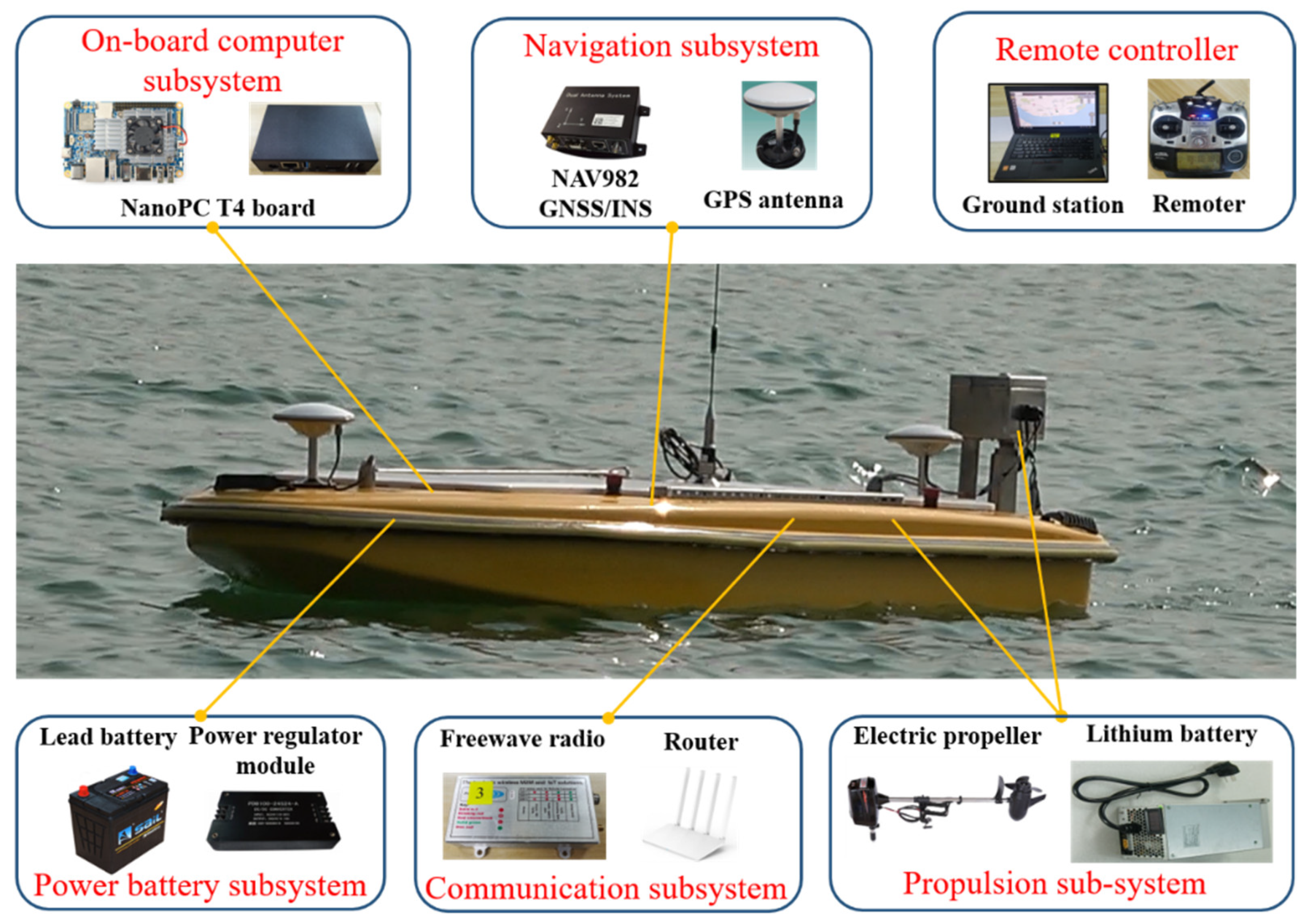
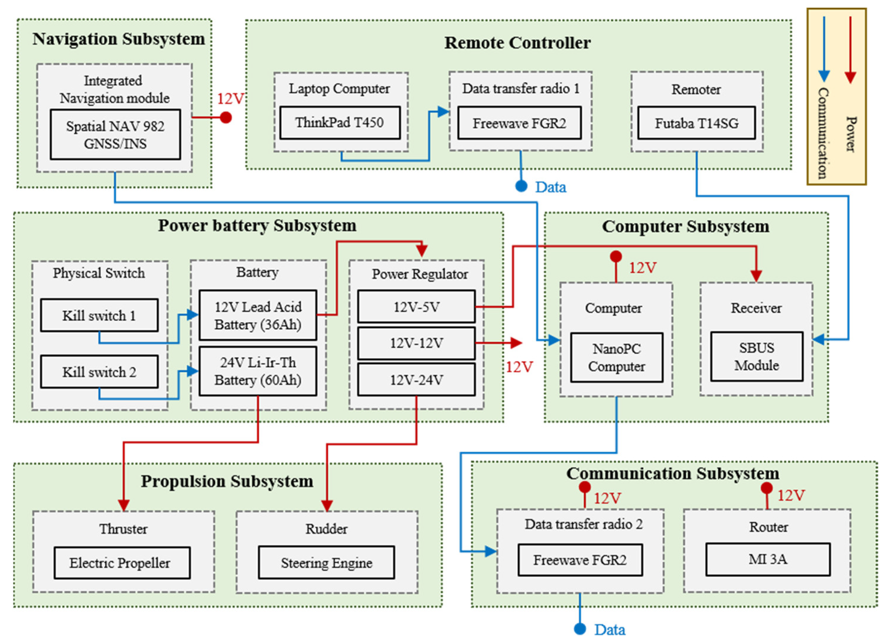
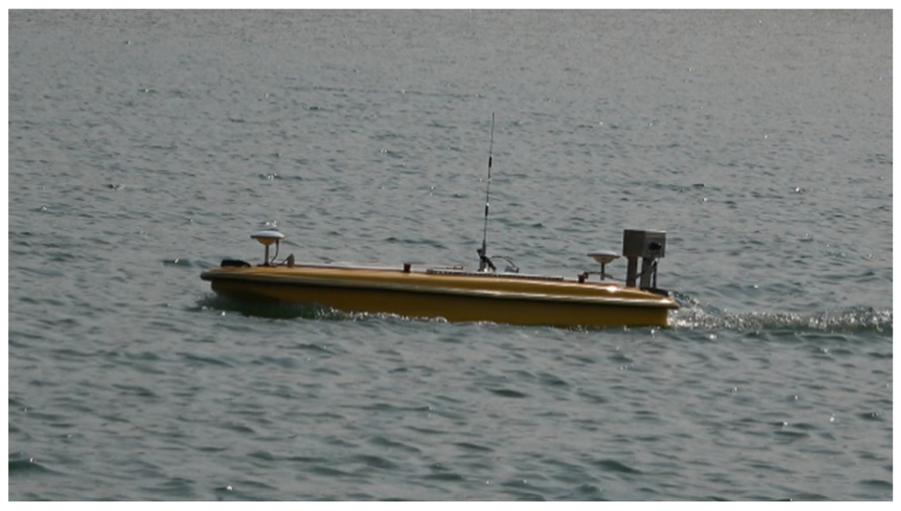
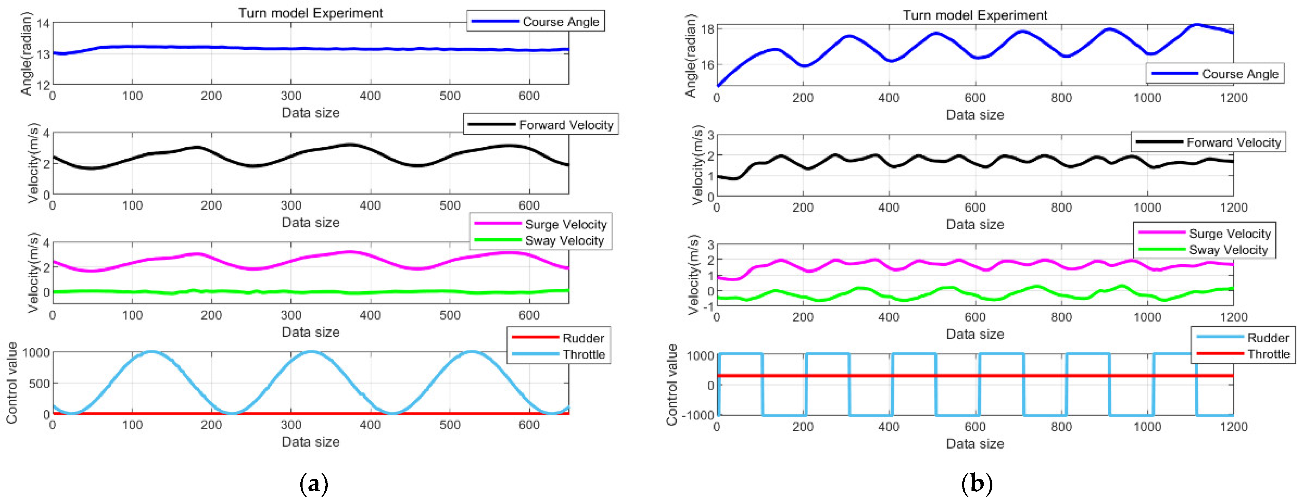
(2) To validate this novel modeling method, we have independently developed the ‘Salmon’ USV experimental platform and conducted groups of system identification experiments in a lake. The USV is equipped with a high-precision integrated navigation system and an automated control system, to guarantee the authenticity, precision, and number of experimental data samples. The efficacy of the method was verified by comparing its performance with other typical and state-of-the-art modeling methods.

1.2. Outline

This study provides a comprehensive overview of the GBM-ILM method, which combines an incremental learning network with a physical mechanism model for learning the USV’s kinetic model. The remainder of the article is structured as follows: Section 2 introduces the related works on USV kinetic modeling. Section 3 details the GBM-ILM method, based on the physical mechanism and incremental learning network, to capture the USV’s kinetics. In Section 4, we introduce the self-developed USV experimental platform and outline the system identification experiments. Section 5 presents a thorough analysis and discussion of the experimental results, comparing the accuracy and effectiveness with other typical modeling methods. Finally, Section 6 provides the conclusions and summarizes key findings.

2. Related Works

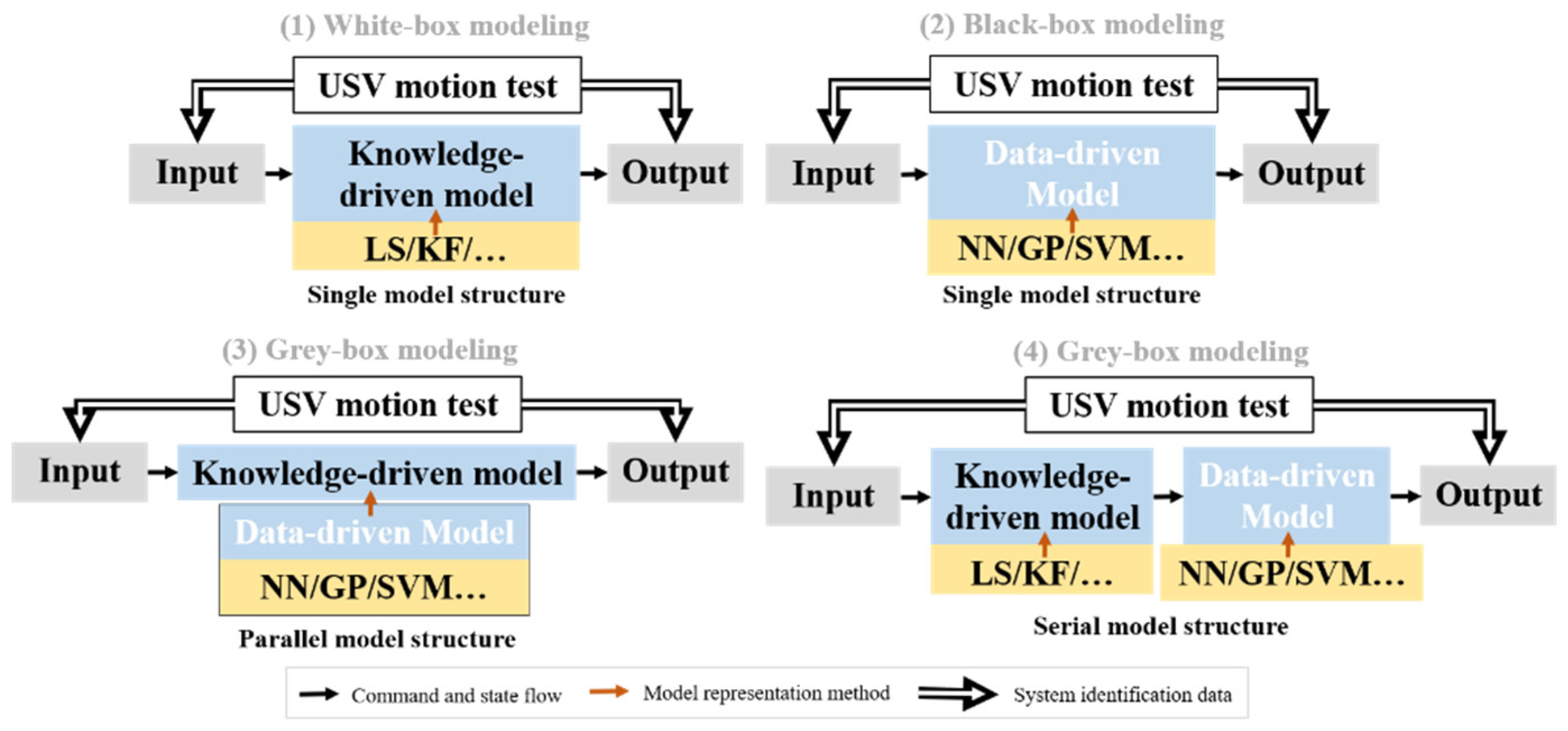
Generally, approaches to system dynamics modeling can be categorized into three types. The first is white-box modeling, also known as a knowledge-driven model, which is shown in Figure 1(1), where the model’s structure is perfectly delineated based on prior knowledge and physical principles. Here, the reference models rely on well-understood and explicitly defined ‘standard’ equations, and the model parameters are obtained by identification algorithms. The second is black-box modeling, also known as a data-driven model, which is shown in Figure 1(2), where the systems do not necessarily offer explicit ‘standard’ equations to describe system dynamics. These models are often stochastic and estimated by multiple learning algorithms. The third is grey-box modeling, combining white-box and black-box modeling, which is shown in Figure 1(3,4). In grey-box modeling, its hybrid structure explores the functional relationships between the input, output, and estimated values (derived from the white-box model) by employing the black-box model [14,15].

White-box modeling has been rapidly researched and widely used for a long time. In this approach, models are meticulously crafted based on known kinematic and kinetic theories. These models account for a range of factors affecting a USV, such as hydrodynamic forces, control forces, and environmental disturbances. Notable models in this category include the first-order Nomoto model [16], the Abkowitz model [17], a mathematical maneuvering model [18], the Manoeuvring Modeling Group (MMG) model [19], and a six degree-of-freedom (six-DOF) nonlinear kinetics model and its deformation models [20,21]. The structures of these models are well-defined, and unknown parameters can be obtained by various system identification methods. One of the most popular parameter identification methods is the Kalman filter (KF) [22,23] and its variants, such as the extended Kalman filter (EKF) [24,25] and the unscented Kalman filter (UKF) [26,27,28]. Another popular method for parameter identification is the least squares (LS) method [29,30,31,32]. White-box models are typically derived from expert knowledge; however, partial studies tend to oversimplify specific dynamic properties or assume that the USV system operates under time-invariant conditions (in calm waters) [14,33]. Furthermore, the model’s effectiveness is often constrained by the researchers’ limited prior physical knowledge of the USV’s dynamic characteristics, as well as their observational capacity during maneuvering. These limitations can compromise the model’s accuracy and adaptability to changes in both internal states and external environmental factors, such as payload variations, structural changes, wind, waves, and currents [34].

Black-box modeling is an approach for systems whose structures and mechanisms are completely unknown. This method establishes an optimal mapping relationship between input and output data, bypassing the need for any prior physical knowledge of the explicit mathematical model that reflects the system’s dynamic characteristics. Artificial neural networks (ANNs) are commonly employed in black-box modeling [35,36], such as two-layer fully connected neural networks [37], three-layer feedforward neural networks with Chebyshev orthogonal basis functions [38], generalized ellipsoidal basis function fuzzy neural networks [39], long short-term memory (LSTM) [40], recursive neural networks [41], and deep learning networks [42]. These architectures aim to map the dynamic relationship between input state variables and output variables such as hydrodynamic force and moment, identifying nonlinear functions in the process. Another prevalent technology in this domain is the kernel-based method, which relies on statistical approaches. This technique maps training data into a high-dimensional feature space using a kernel trick, circumventing the need for physical insight into the system [43]. By doing so, it more effectively captures the nonlinear relationship between input and output data. In the kernel-based methods, support vector machines (SVMs) and the Gaussian process (GP) have attracted widespread interest. SVMs have been used in various studies [44,45,46]; additionally, a variant of SVM, known as the least square support vector machine (LSSVM) [47], aimed to minimize both the empirical risk (i.e., estimation error in the training data) and structural risk (i.e., model complexity) [48,49,50,51,52]. In contrast, GP regression operates as a Bayesian learning method rooted in kernel functions. Unlike SVMs, which generally excel in limited sample scenarios, the GP provides an intuitive confidence interval for output results, thus offering insights into their reliability. The model produced through GP regression is probabilistic; thus, it has both universality and solvability. The GP has been used in various studies [53,54,55,56,57,58]. However, these kernel-based modeling approaches often lack a strong theoretical underpinning, due to the absence of rational physical laws [56,57]. In practical applications involving USVs, the model’s performance is subject to significant uncertainties. This is because both the state of the USV system and the external environmental factors are continually changing, leading to outdated data, exceeding of the model’s applicability, or a loss in efficacy [59].

Contrary to white-box and black-box modeling, grey-box modeling can synthesize the advantages of both approaches, by not only optimizing the identification coefficients of complex systems but also fully accounting for the mechanism of USV maneuvering. In parallel grey-box modeling, Wang et al. [15] introduced a grey-box model based on a SVM, utilizing a third-order Taylor expansion as an alternative to the MMG and Abkowitz model structures. However, this model overlooked hydrodynamic coefficients and suffered from extended computation times. Similarly, Mei et al. [60] proposed a grey-box framework for modeling ship maneuvering using an MMG model, random forest (RF), and a SVM. They employed fewer free-running model test data and utilized the SVM technique to identify the MMG model parameters through a tightly coupled approach. Chen et al. [61] advanced a four-DOF grey-box model for ship maneuvering based on the MMG model and LSSVM. However, their focus remained solely on the kinetics of the USV, identifying only the relationship between established white-box models and black-box methods. Reference model parameters can be dynamically adjusted using black-box techniques, although these are susceptible to large errors in changeable experimental environments. In serial grey-box modeling, our previous research combined a linear parameter-varying (LPV) model with the UKF to estimate the kinetic model of the USV. The limitation here is that the UKF parameters had to be predetermined and that the model error was assumed to be noise-driven [62]. Thus, the model had poor adaptability to datasets from different times or mutable environments. A critical research focus in grey-box modeling for USVs is the need for models to adapt to changing environmental conditions and system states in real-time. This is crucial to rationally divide the white and black parts and avoid the existing problems of both models.

The major publications in recent years within the USV modeling research field are listed in

Table 1. Major relevant research on USV kinetic modeling in recent years.

References	Model	Algorithm	Mode
Sonnenburg and Woolsey (2013) [12]	White-box	LS	Offline
Luo et al. (2014) [44]	Black-box	SVM	Offline
Zhang et al. (2015) [29]	White-box	LS	Offline
Xu and Guedes Soares (2016) [48]	Black-box	LSSVM	Offline
Han et al. (2017) [62]	Grey-box	LPV + UKF	Online
Ariza Ramirez et al. (2018) [53]	Black-box	GP	Offline
Woo et al. (2018) [42]	Black-box	LSTM-ANN	Offline
Mei et al. (2019) [60]	Grey-box	MMG + RF	Offline
Xu et al. (2020) [52]	Black-box	LSSVM	Online
Zhu et al. (2020) [49]	Black-box	LSSVM	Offline
Dimitrov et al. (2021) [40]	Black-box	LSTM-ANN	Offline
Alexandersson et al. (2022) [25]	White-box	EKF	Online
Chen et al. (2022) [61]	Grey-box	MMG + LSSVM	Offline
Shen et al. (2022) [27]	White-box	UKF	Online
Wang et al. (2022) [23]	White-box	GP	Online
Xue et al. (2022) [56]	Black-box	GP	Online
Yue et al. (2022) [22]	White-box	KF	Online
Liu et al. (2023) [58]	Black-box	GP	Offline

. Based on the analysis of the above-mentioned literature, simplified mechanism models decrease accuracy due to their omission of uncertainty, while data-driven network models result in errors out of their scope. Additionally, models derived from offline experimental data struggle to adapt to dynamic environments. This is because the offline data are time-invariant and fail to capture changes in the state of the USV, leading to limitations in the models’ generalizability and adaptability. Therefore, there is an urgent need for an intelligent method that can dynamically and accurately estimate the USV kinetic model online, while considering uncertainties and changes in both the internal USV systems and the external environment.

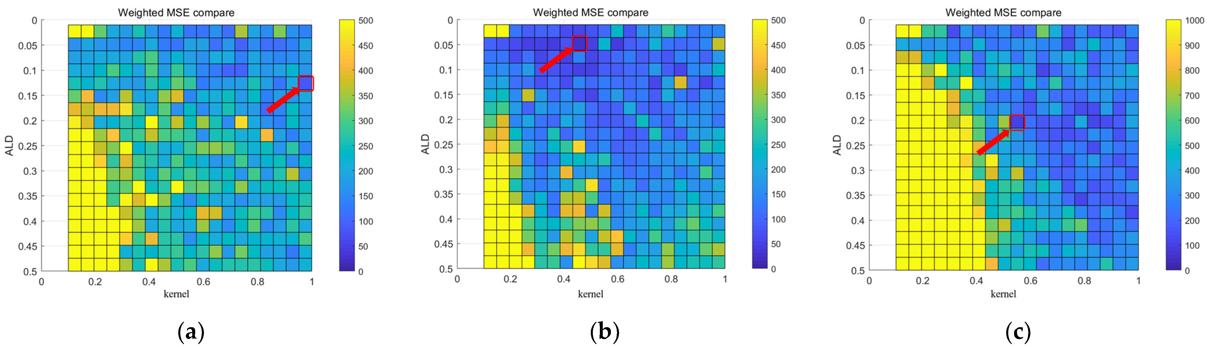
Inspired by previous studies, this study introduces a novel grey-box modeling method that combines incremental learning with a mechanism model. This approach actively calculates model errors in real-time, identifying them as unmodeled parts. Simultaneously, to ensure adaptability to time-varying environmental conditions and USV states, it fits these model errors using an incremental learning network, which can continuously update both its structure and parameters by iteratively incorporating new data. This compensates for the shortcomings of the mechanism model and improves the overall modeling accuracy. The heart of the incremental learning network is the kernel recursive least squares with approximate linear dependency (KRLS-ALD) algorithm [63]. This algorithm solves the nonlinear inseparability problem by projecting input data into the reproducing kernel Hilbert space. This enables the establishment of a quick and accurate online model adaptable to changing conditions. The approximate linear dependency (ALD) formula can determine whether the input data are new to the incremental learning network model [64]. In summary, this study not only makes the USV kinetic model interpretable but also determines the boundaries for model errors. Building on this foundation, it estimates and compensates for model error using incremental learning, thereby enhancing the precision of USV dynamic modeling. The main parameters in the article are explained in

Table 2. The nomenclature of main parameters in this article.

Parameters	Definition	Parameters	Definition
$(x_g,y_g)$	USV’s gravity center	$m$	Mass of the USV [kg]
$u,v,r$	Velocities of surge, sway, and yaw rate [m/s; rad/s]	$x_{\delta }$	Longitudinal moment from center to pivot point
$\psi$	Course angle [rad]	$\beta$	Sideslip angle [rad]
$\delta$	Rudder angle [rad]	$T$	Resultant thrust force [N]
$\dot{u},\dot{v},\dot{r}$	Acceleration of the surge, sway, and yaw motions [m/s2; rad/s2]	$X_{\sum },Y_{\sum },N_{\sum }$	Resultant forces and torque exerted on USV [N]
${\mathit{I}}_{zz}$	Yaw moment of inertia with Z-axis [kg·m2]	$\mathit{\theta }(\mathit{t})$	LPV parameter value
$\mathbf{w}$	Weight matrix	$\mathbf{\Phi }(\mathit{x})$	Mapping function
$x_i\dots x_t$	State input	$y_i\dots y_t$	Prediction output
${\delta }_t$	ALD condition	$\sigma$	Kernel width
$k(x·x)$	Kernel function	${\mathbf{K}}_t$	Kernel matrix

.

3. The Grey-Box Modelling-Incremental Learning and Mechanism (GBM-ILM) Method

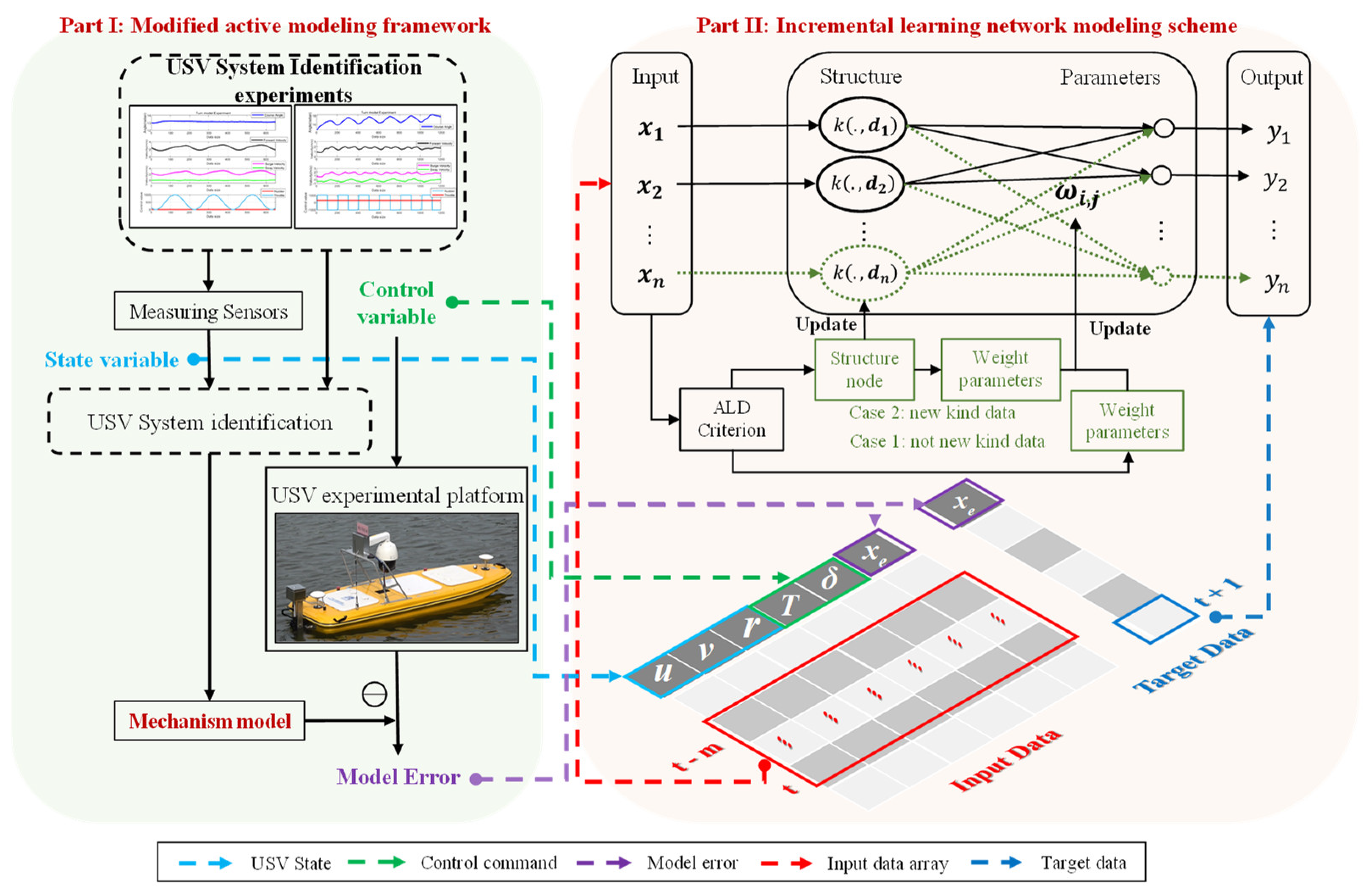
We propose the GBM-ILM method with a novel hybrid modeling framework, outlined in Figure 2, which aims to guarantee both the physical rationality and accuracy of the USV kinetic model. The flow graph of this modified active modeling and incremental learning network based on KRLS-ALD is divided into two parts. In Part I, we introduce a modified active modeling framework, where a structured model is fixed, building on previous research in Section 3.1. The onboard computer and operator can relay desired commands to drive the practical USV system. Simultaneously, multiple sensors attached to the USV continuously measure real-time position and attitude data, the mechanism model also estimates an idealized USV state obtained, and the unforeseeable model error is calculated in this framework, as described in Section 3.2.1. Part II delves into the KRLS-ALD network model, which fits and estimates the model error from Part I. The parameters and structure of this network model are designed to be incrementally updated, as described in Section 3.2.2. This network model can update its structure and parameters by learning new kinds of data from changeable environments and USV states. The dotted line of each color describes how training and testing datasets are transferred from the active modeling framework to the network model. This method provides the USV states, USV control commands, and model errors as input data, with the model error serving as the target data for network training. The input dataset comprises either a set of synchronous values or a series of consecutive historical moments, as described in Section 3.2.3. With the training of this network model, its ability to predict the model error is gradually enhanced; this incremental learning strategy thrives even with limited samples, unlike other traditional machine learning theories, which rely on large sample sizes. As both the USV system and its environment change, the amount of data increases, and the network model keeps constantly updating.

3.1. Unmanned Surface Vehicle (USV) Mechanism Model

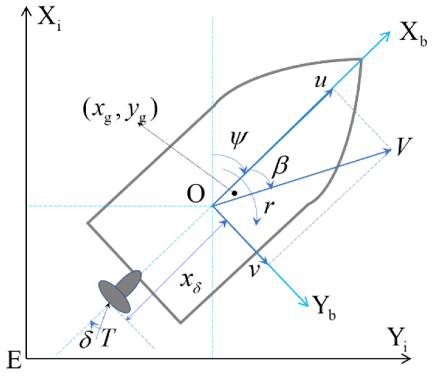
Generally, USV kinetics are commonly defined as surge, sway, heave, roll, yaw, and pitch, as enacted by the Society of Naval Architects and Marine Engineers (SNAME). In this study, to streamline our analysis, we focus solely on three-DOF—surge, sway, and yaw—to describe the USV’s horizontal planar motion, neglect heave, roll, and pitch motions; the USV coordinate frames are illustrated in Figure 3.

3.1.1. Basics of Unmanned Surface Vehicle Modeling

According to [21], the detailed three-DOF kinetic model for a USV is as follows:

$$\begin{array}{r}m(\dot{u}-y_{\mathrm{g}}\dot{r}-vr-x_{\mathrm{g}}{r}^2)=X_{\sum }\\ m(\dot{v}+x_{\mathrm{g}}\dot{r}+ur-y_{\mathrm{g}}{r}^2)=Y_{\sum }\\ I_{zz}\dot{r}+m\left[x_{\mathrm{g}}(\dot{v}+ur)-y_{\mathrm{g}}(\dot{u}-vr)\right]=N_{\sum }\end{array}$$

(1)

On the USV, external forces are divided into two sections: hydrodynamic forces and thrust forces. The resultant forces in the surge, sway, and yaw are dependent on the USV motion states, the forces, and torque produced by the thruster. These can be described using the following equations:

$$\begin{array}{l}{X}_{\sum }=X_{\mathrm{hydro}}+X_{\mathrm{ctrl}}+X_{\mathrm{dis}}\\ Y_{\sum }=Y_{\mathrm{hydro}}+Y_{\mathrm{ctrl}}+Y_{\mathrm{dis}}\\ N_{\sum }=N_{\mathrm{hydro}}+N_{\mathrm{ctrl}}+N_{\mathrm{dis}}\end{array}$$

(2)

where $X_{\mathrm{hydro}}$, $Y_{\mathrm{hydro}}$, and $N_{\mathrm{hydro}}$ are hydrodynamic forces, while $X_{\mathrm{ctrl}}$, $Y_{\mathrm{ctrl}}$, and $N_{\mathrm{ctrl}}$ are thrust forces. The resisting forces and torque can be represented using polynomial equations [65], which are given in Appendix A. Generally, USVs are designed with lateral symmetry, by letting $y_g=0$, $v={\left[u,v,r\right]}^{\mathrm{T}}$, and substituting Equation (2) into Equation (1) allows us to rewrite Equation (1) as follows:

$$\mathbf{M}\dot{\mathit{v}}=\mathbf{N}\left(\mathit{v}\right)\mathit{v}+{\mathbf{F}}_{\mathrm{ctrl}}$$

(3)

where $\mathbf{M}=\left[\begin{array}{ccc}m-X_{\dot{u}}& 0& 0\\ 0& m-Y_{\dot{v}}& m{x}_g-Y_{\dot{r}}\\ 0& m{x}_g-N_{\dot{v}}& I_{zz}-N_{\dot{r}}\end{array}\right]$, $\mathbf{N}(v)=\left[\begin{array}{ccc}{X}_{\left|u\right|u}\left|u_r\right|+X_u& (m+X_{vr})r& (m{x}_g+X_{rr})r\\ -mr& Y_{\left|v\right|v}\left|v\right|+Y_v& Y_{\left|v\right|r}\left|v_r\right|+Y_r\\ m{x}_{g}r& N_{\left|v\right|v}\left|v\right|+N_v& N_{\left|v\right|r}\left|v_r\right|+N_r\end{array}\right]$.

Obviously, the thrust force equations are derived as follows:

$${\mathbf{F}}_{\mathrm{ctrl}}={\left[X_{\mathrm{ctrl}}{Y}_{\mathrm{ctrl}}{N}_{\mathrm{ctrl}}\right]}^{\mathrm{T}}={\left[T\cos \delta -T\sin \delta T{x}_{\delta }\sin \delta \right]}^{\mathrm{T}}$$

(4)

Thrust $T$ is a function of the forward velocity $u$($u>0$) and propeller speed ${\delta }_{\mathrm{n}}$ [20], as follows:

$$T=b_1\left|{\delta }_{\mathrm{n}}\right|{\delta }_{\mathrm{n}}+b_2\left|{\delta }_{\mathrm{n}}\right|u=k_1{\epsilon }^{2/3}+k_2{\epsilon }^{1/3}u$$

(5)

where $\epsilon$ is the propeller throttle value, and $b_1$, $b_2$, $k_1$, and $k_2$ are constants.

3.1.2. Thrust and Steering Models

This section introduces two prominent linear models. In many existing studies, a linearized model serves as an approximation to describe the dynamics of the USV system. In the forward motion condition, we assumed that the yaw rate $r=0$, the sway velocity $v=0$, and the forward velocity $u=u_0$ [62]. Equation (3) can be linearized as follows:

$$\mathbf{M}\dot{\mathit{v}}={\mathbf{N}}_1\mathit{v}+{\mathbf{F}}_{\mathrm{ctrl}}$$

(6)

where ${\mathbf{N}}_1$ is a reduced matrix that replaces $\mathbf{N}\left(\mathit{v}\right)$, as follows:

$${\mathbf{N}}_1=\left[\begin{array}{ccc}{X}_{\left|u\right|u}\left|u_r\right|+X_u& 0& 0\\ 0& Y_v& Y_r-m{u}_0\\ 0& N_v& N_r-m{x}_g{u}_0\end{array}\right]$$

(7)

It is worth noting that the surge motion can generally be decoupled from the sway–yaw subsystem when the forward speed remains constant or changes within a limited range. Thus, Equation (6) can be readily linearized in its perturbed form as follows:

$$\mathsf{\Delta }\dot{u}=a\mathsf{\Delta }u+b\mathsf{\Delta }T$$

(8)

$$\left[\begin{array}{c}\dot{v}\\ \dot{r}\end{array}\right]=\left[\begin{array}{cc}{a}_{11}& a_{12}\\ a_{21}& a_{22}\end{array}\right]\left[\begin{array}{c}v\\ r\end{array}\right]+\left[\begin{array}{c}{b}_1\\ b_2\end{array}\right]T\delta$$

(9)

where $\mathsf{\Delta }u=u-u_0$, $\mathsf{\Delta }T=T-T_0$, and $T_0$ is the constant thrust force of the USV; other coefficients, namely $a_{ij}(i=1,2;j=1,2)$ and $b_k(k=1,2)$, are given in Appendix B.

The Nomoto model can be described as follows:

$$r(s){\delta }^{-1}(s)=K_r(T_{3}s+1){\left[(T_{1}s+1)T_{2}s+1\right]}^{-1}$$

(10)

where $T_1{T}_2=1/(a_{11}{a}_{22}-a_{12}{a}_{21})$, $T_1+T_2=-(a_{11}+a_{22})/(a_{11}{a}_{22}-a_{12}{a}_{21})$, $T_3=b_2/(a_{21}{b}_1-a_{11}{b}_2)$, and $K_r=\left[(a_{21}{b}_1-a_{11}{b}_2)T_0\right]/(a_{11}{a}_{22}-a_{12}{a}_{21})$.

The relationship between $\delta$ and $r$ can be described as a simple function [16], as follows:

$$r(s){\delta }^{-1}(s)=K_r{\left[(T_1+T_2-T_3)s+1\right]}^{-1}$$

(11)

When the USV’s heading suffers minor perturbations, the sideslip angle $\beta \ne 0$. Assuming that the forward velocity remains unchanged and the yaw perturbations are small, the resultant thrust $F_{\sum }$ acts in the direction opposite to the resultant velocity $V$. Under these assumptions, the dynamics of sway are formulated as $m\dot{v}+mur=-F_{\sum }\sin \beta$. Letting $u=V\cos \beta$ and $v=V\sin \beta$, we obtain the following:

$$T_{\beta }\dot{\beta }+\beta =-K_{\beta }r$$

(12)

where $T_{\beta }=mV/F_{\sum }$ and $K_{\beta }=mV/F_{\sum }$. By combining Equations (11) and (12), a fully linearized steering model is obtained, as follows:

$$\left[\begin{array}{c}\dot{\beta }\\ \dot{r}\end{array}\right]=\left[\begin{array}{cc}-1/T_{\beta }& -1\\ 0& -1/T_r\end{array}\right]\left[\begin{array}{c}\beta \\ r\end{array}\right]+\left[\begin{array}{c}0\\ K_r/T_r\end{array}\right]\delta$$

(13)

Equation (13) is known as the linear model (Nomoto), considering sideslip motion.

3.1.3. Linear Parameter-Varying Model

According to the existing literature [66], an LPV system is usually defined as a linear system with state-space representations that depend on some external variable $\mathit{\theta }(t)$. The system can be described by the following equation:

$$\dot{\mathit{v}}=A\left[\mathit{\theta }(t)\right]\mathit{v}+B\left[\mathit{\theta }(t)\right]\mathit{u}$$

(14)

where the scheduling variable $\mathit{\theta }(t)$ is a priori unknown but can be measured online. If the function $\mathit{\theta }(t)$ contains states from the state vector $\mathit{v}$, then Equation (14) is called an LPV model [67]. In other words, LPV systems consist of an indexed collection of linear systems, where the indexing parameter is endogenous, as it depends on the system’s state.

The nonlinear model of the USV system, as shown in Equation (6), includes many parameters that are strongly coupled and difficult to identify through real-world experiments. Extracting the nonlinear structure of the USV system for conversion into an LPV form proves difficult. In this section, we re-analyze Equation (6), to show that it can be transferred into the following LPV format:

$$\dot{\mathit{v}}=A(\mathit{v})\mathit{v}+B\mathit{u}$$

(15)

where $A(\mathit{v})=M^{-1}N(\mathit{v})$, $\mathit{u}=T{\left[\sin \delta \cos \delta \right]}^{\mathrm{T}}$, and $B=M^{-1}{\left[\begin{array}{ccc}\begin{array}{c}0\\ 1\end{array}& \begin{array}{c}-1\\ 0\end{array}& \begin{array}{c}{x}_{\delta }\\ 0\end{array}\end{array}\right]}^{\mathrm{T}}$.

The LPV model structure represents an alternative formulation of the physical system model for the considered hydrodynamics of the USV. Its key advantage lies in presenting the nonlinear system structure in a form akin to a special type of linear structure, offering the following two benefits: (1) its parameters can be identified using linear algorithms, thereby yielding a nonlinear mathematical model, and (2) well-established linear control synthesis techniques can be applied and adapted to achieve satisfactory performance.

3.2. Incremental Learning Model

3.2.1. Modified Active Modeling Framework

While three-DOF kinetic models offer a certain level of insight, achieving precise parameter values remains challenging, due to their time-varying characteristics and the inherent uncertainty involved. To address these issues, this study employs an active modeling technique to estimate the model error, treating the unstructured factors in the USV system. The active modeling framework regards these unstructured models as unknown disturbances, obtaining them through an online estimator. Numerous studies validate the effectiveness of active modeling in real-world system control. The main idea of the active modeling technique is the description of a system, using the following system equation:

$$\dot{\mathit{x}}=\mathit{f}(\mathit{x},\mathit{u})+\mathsf{\Delta }\mathit{f}$$

(16)

where $\mathit{x}$ is the state of the system; $\mathit{u}$ is the input of the system; $\mathit{f}$ is the nonlinear structured model function; and $\mathsf{\Delta }\mathit{f}$ is the model error vector, which includes all the factors of the unstructured model mismatch (i.e., model imprecision and external disturbances) and may relate to the system state $\mathit{x}$ or even the control input.

In this framework, Equation (16) is combined with a predefined structured model and unstructured model errors to describe the dynamic characteristics of the system under control. The structured model serves as the foundation for designing a nominal controller, while the estimated model error can be combined with adaptive schemes to improve the closed-loop performance of that controller. To obtain the model error, we rewrite the system Equation (15) to conform to the state-space format of Equation (16), as follows:

$$\dot{\mathit{v}}=\mathit{Av}+\mathit{Bu}+\mathsf{\Delta }\mathit{v}$$

(17)

where $\mathit{v}$ is the system state vector, $\mathit{Av}+\mathit{Bu}$ represents the structured system dynamics as shown in Equations (15), and $\mathsf{\Delta }\mathit{v}$ is the model error.

3.2.2. Kernel Recursive Least Squares–Approximate Linear Dependency (KRLS–ALD) Algorithms

In the context of the incremental learning method, we employed a simplified form of the RLS algorithm to minimize the sum of the squared errors at each time step [63], as follows:

$$L(\mathbf{w})={\displaystyle \sum _{i=1}^t{(\mathit{f}({\mathit{x}}_i)-y_i)}^2}={\Vert {\mathbf{\Phi }}_t^{\mathrm{T}}\mathbf{w}-{\mathit{y}}_t\Vert }^2$$

(18)

where ${\mathit{x}}_i={(x_1,\dots ,x_t)}^{\mathrm{T}}$ is the USV state input, and ${\mathit{y}}_t={(y_1,\dots ,y_t)}^{\mathrm{T}}$ is the prediction vector. The kernel function is utilized as $k(\mathit{x},\mathit{d})=\langle \mathit{\varphi }(\mathit{x}),\mathit{\varphi }(\mathit{d})\rangle =k(\Vert \mathit{x}-\mathit{d}\Vert )$, wherein $\mathit{d}$ is the central vector of the network, $\mathit{\varphi }(\cdot )$ maps $x$ into a higher-dimensional Hilbert space, and ${\mathbf{\Phi }}_t=\left[\mathit{\varphi }(x_1),\dots ,\mathit{\varphi }(x_t)\right]$, within considering the residual component vector.

Typically, we would minimize Equation (18) with respect to $\mathbf{w}$ and to obtain ${\mathbf{w}}_t=\arg {\min }_{\mathbf{w}}{\Vert {\mathbf{\Phi }}_t^{\mathrm{T}}\mathrm{w}-{\mathit{y}}_t\Vert }^2={({\mathbf{\Phi }}_t^{\mathrm{T}})}^{†}{\mathit{y}}_t$, where ${(\cdot )}^{†}$ denotes the pseudo-inverse. The classical RLS algorithm, as described by [68], leverages the matrix inversion lemma to minimize the loss $L(\mathbf{w})$ online, eliminating the need to recompute the matrix ${({\Phi }_t^{\mathrm{T}})}^{†}$ at each step.

It is worth noting that the feature space could have very high dimensionality, which makes matrix manipulations computationally intensive, especially for matrices such as ${\Phi }_t$. However, as can be easily verified, the optimal weight vector can be expressed in a more tractable form, as follows:

$${\mathbf{w}}_t={\displaystyle \sum _{i=1}^t{\alpha }_i\mathit{\varphi }({\mathit{x}}_i)={\mathbf{\Phi }}_t\mathit{\alpha }}$$

(19)

where $\mathit{\alpha }={({\alpha }_1,\dots ,{\alpha }_t)}^{\mathrm{T}}$. Substituting this into Equation (18) and altering the notation, we obtain the following equation:

$$L(\mathit{\alpha })={\Vert {\mathbf{K}}_t\mathit{\alpha }-{\mathit{y}}_t\Vert }^2$$

(20)

where ${\mathbf{K}}_t=k(x_t,x_t)$. The optimal solution to Equation (20) is given in Appendix C.

In order to adapt to dynamic changes in network structure, we integrate ALD criterion into the kernel recursive least squares (KRLS) algorithm [64]. For the approximate linear dependency (ALD) formula [69], assuming that the USV obtains ${\mathit{x}}_t$, and dictionary is ${\mathit{D}}_{t-1}$, the number of nodes is $m_{t-1}$.

$${\delta }_t=k_{tt}-{\mathit{k}}_{t-1}^{\mathrm{T}}({\mathit{x}}_t){\mathit{k}}_{t-1}^{-1}{\mathit{k}}_{t-1}({\mathit{x}}_t)\le \mu$$

(21)

We consider one of two scenarios in an online scenario at each time step, as follows:

(1) $\varphi ({\mathit{x}}_t)$ is the ALD on ${\mathit{D}}_{t-1}$, i.e., ${\delta }_t\le \mu$ and ${\mathit{a}}_t={\tilde{\mathbf{K}}}_{t-1}^{-1}{\tilde{\mathbf{k}}}_{t-1}(x_t)$. In this case, ${\mathit{D}}_t={\mathit{D}}_{t-1}$, $m_t=m_{t-1}+1$, and ${\tilde{\mathbf{K}}}_t={\tilde{\mathbf{K}}}_{t-1}$.

(2) ${\delta }_t>\mu$, and, therefore, $\varphi ({\mathit{x}}_t)$ is not ALD on ${\mathit{D}}_{t-1}$. ${\mathit{x}}_t$ is added to the dictionary, i.e., ${\mathit{D}}_t={\mathit{D}}_{t-1}\cup \left\{{\mathit{x}}_t\right\}$, $m_t=m_{t-1}+1$, and ${\tilde{\mathbf{K}}}_t$ grows accordingly.

The KRLS update equations derived are given in Appendix D.

For the final equality, we use ${\mathit{a}}_t^{\mathrm{T}}{\tilde{\mathbf{K}}}_{t-1}={\tilde{\mathit{k}}}_{t-1}{({\mathit{x}}_t)}^{\mathrm{T}}$. The network prediction output about state ${\mathit{x}}_t$ can be normalized as follows:

$${\mathit{y}}_{t+1}={\mathbf{w}}_t{\mathbf{K}}_t({\mathit{x}}_t)$$

(22)

3.2.3. Model Error Prediction

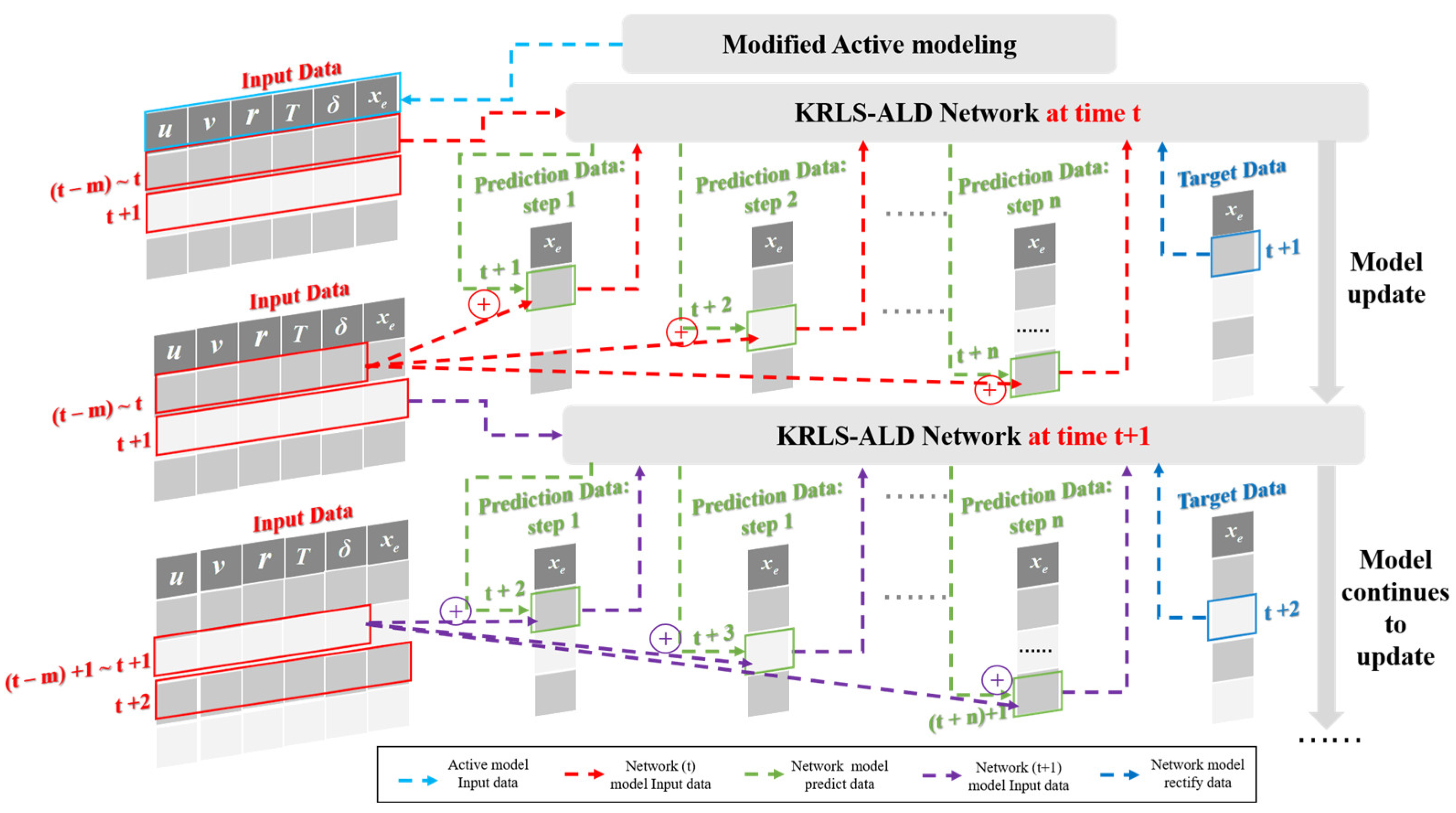
In this GBM-ILM method, the network can estimate model errors by means of iterative prediction. As shown in Figure 4, firstly, at time $t$, the input data are obtained from the active modeling framework; it predicts $x_{\mathrm{e}}$ at time $t+1$ using the network model in the inner loop. Secondly, in the same step, the network iteratively predicts $x_{\mathrm{e}}$ for the next time step until it reaches time $t+n$. Finally, the actual value at time $t+1$ serves to adjust the network. Using this flow, the network model can predict model errors in future time, thereby estimating the entire USV’s kinetic model, which can be put into navigation and control.

Through Equation (22), the model error prediction function is undertaken as follows:

$${\mathrm{y}}_{t+1}=w_t{K}_t({\mathit{x}}_t,{\mathit{x}}_{t-1},{\mathit{x}}_{t-2}\dots ,{\mathit{x}}_{t-m})$$

(23)

where ${\mathit{x}}_i={\left[u_i{v}_i{r}_i{T}_i{\delta }_i{\mathit{x}}_{\mathrm{e}i}\right]}^{\mathrm{T}},i=t,t-1,\dots ,t-m$, and the input data include USV’s state $(u,v,r)$, control input $(T,\delta )$, and model error ${\mathit{x}}_{\mathrm{e}}$, which all come from the system identification experiments on the USV platform, as described in Section 4.

4. Unmanned Surface Vehicle System Model Identification

To verify the effectiveness and accuracy of our proposed GBM-ILM method in USV kinetic modeling, a real-world USV equipped with accurate state measurement capabilities is essential. Additionally, it is imperative to collect a large amount of field experiment data under suitable water conditions. These data will be utilized for real-time model estimation and prediction through the incremental learning network.

4.1. Unmanned Surface Vehicle Platform Setup

Our research group—the Autonomous Robot Group, State Key Laboratory of Robotics, Shenyang Institute of Automation, Chinese Academy of Sciences (SIA, CAS)—has developed the ‘Salmon’ USV experimental platform. The main parameters of this USV are shown in

Table 3. Main characteristic parameters of ‘Salmon’ USV.

Mass	Length	Breadth	Height	Minimum Turning Radius
70 kg	2.6 m	0.8 m	0.7 m	1.5 m

.

Built with a modular design, each subsystem is responsible for different working tasks; the developed USV experimental platform is shown in Figure 5. The hardware system mainly comprises six main subsystems: (1) onboard computer, (2) navigation, (3) remote controller, (4) power battery, (5) communication, and (6) propulsion.

The USV’s hardware architecture is described in Figure 6.

For the accuracy of the location and navigation data within the system identification dataset, we installed a specialized navigation subsystem on the USV. This subsystem is designed to continuously measure the USV’s spatial position, including both location and orientation. To achieve this, we equipped the USV platform with a NAV982 Global Navigation Satellite System Inertial Navigation System (GNSS/INS) integrated navigation module along with two Global Position System (GPS) antennas. This module offers horizontal position accuracy within 0.5 m and vertical position accuracy within 0.8 m. It rapidly delivers raw navigation and location information at a 20 Hz frequency to the onboard computer, enabling precise navigation during system identification missions in open water areas. The key performance parameters for the NAV982 GNSS/INS integrated navigation module are listed in

Table 4. Main parameters of navigation system.

Horizontal Position Accuracy	Vertical Position Accuracy	Velocity Accuracy	Course Accuracy	Pitch/Roll Accuracy	Sampling Frequency
0.5 m	0.8 m	0.007 m/s	0.1°	0.2°	20 Hz

.

To ensure precise navigation capabilities for the USV in open water areas, we designed multiple control strategies for the hardware system, all running within the Ubuntu operating system on the USV’s computer subsystem. Following the modular, multithreaded design ideology, the software system is organized into the following four main parts: (1) the tasks module, which defines detailed action plans for each identification task; (2) the control module, which serves as the highest level of the software structure; (3) the communication module, which is responsible for linking sensors, controllers, and equipment; and (4) the devices module, which includes both navigation and control hardware. The software structure of the developed USV is graphically described in Figure 7.

4.2. Unmanned Surface Vehicle System Identification Experiments

4.2.1. Identification Experiments Process

To minimize external influence, we conducted identification experiments at the Shui Fu Temple Lake. The experimental conditions were carefully selected, as follows: (1) the water depth is 5–25 m, more than eight times the depth of the USV’s mean draught; (2) the wind conditions are rated as two on the Beaufort scale, and the wave height is classified as a sea state degree of one; and (3) the current is uniform throughout the testing area. Notably, while we aimed for the calmest water conditions for our experiments, the USV was designed to operate in conditions up to a sea state degree of two, currents up to 2 m/s, and winds classified as less than three on the Beaufort scale. We carried out two sets of experiments to identify the model parameters. Figure 8 shows the conditions of the identification experiment of the USV platform.

(1) Linear experiment: for thrust model identification, the USV responded to a reference throttle while maintaining a fixed rudder angle; $\epsilon$ changes and $\delta =0$. Under these ideal conditions, the rudder was set to zero, allowing the USV to navigate along a straight path without external disturbance. The throttle input was a step signal, with its maximum value limited to 60% of the full throttle range.

(2) Zigzag experiment: for full-state USV model identification, we varied the rudder angle while keeping the throttle fixed at $\epsilon =$ 30%, 60%, and 100% of its full range and $\delta$ changing. Various USV parameters, including rudder angle $\delta$, throttle $\epsilon$, forward velocity $u$, sideslip velocity $v$, and turn rate $r$, were captured using onboard sensors. The rudder was operated repetitively more than five times during these tests, and data were measured every 5 milliseconds for comprehensive analysis. Figure 9 shows part of the identification experimental data of the USV platform’s state.

4.2.2. Model Identification

The linear systems defined by Equations (8), (9) and (13) can be discretized directly in the following form [70]:

$$\begin{array}{l}x\left[k\right]=A_{d}x\left[k-1\right]+B_{d}u\left[k-1\right]\\ z\left[k\right]=x\left[k\right]+\eta \left[k\right]\end{array}$$

(24)

where $A_d=e^{TsA}$; $B_d={\displaystyle {\int }_0^{T_s}{e}^{At}}dtB$; $A$ and $B$ are the system dynamics and input matrices for the original continuous system, respectively; $\eta$ is the noise uncorrelated with the input $\mathit{u}$; $T_{\mathrm{s}}$ is the sampling period; and $T_{\mathrm{s}}=0.05$ second (s) in the experiment. Model parameters can be derived directly using the LS algorithm, as follows:

$$\widehat{\theta }=Z{H}^{\mathrm{T}}{(H{H}^{\mathrm{T}})}^{-1}$$

(25)

where $\theta =\left[A_{\mathrm{d}}{B}_d\right]$; $Z=\left[z\left[2\right]z\left[3\right]\dots z\left[N\right]\right]$; and $H={\left[\begin{array}{cc}z\left[1\right]z\left[2\right]\dots z\left[N-1\right]& u\left[1\right]u\left[2\right]\dots u\left[N-1\right]\end{array}\right]}^{\mathrm{T}}$.

The explicit expression of the model can be deduced from Equation (15). The thrust model is obtained as follows: $u\left[k+1\right]=a_{11}^{d}u\left[k\right]+a_{12}^d\left|u\left[k\right]\right|u\left[k\right]+b_{11}^{d}T$. For the LPV model, we obtain the following:

$$\begin{array}{l}u\left[k+1\right]=a_{11}^{d}u\left[k\right]+a_{12}^d\left|u\left[k\right]\right|u\left[k\right]+a_{13}^{d}v\left[k\right]r\left[k\right]+a_{14}^d{r}^2\left[k\right]+\tilde{T}\left[k\right]\cos \delta \left[k\right]\\ v\left[k+1\right]=a_{21}^{d}u\left[k\right]r\left[k\right]+a_{22}^{d}v\left[k\right]+a_{23}^d\left|v\left[k\right]\right|v\left[k\right]+a_{24}^{d}r\left[k\right]+a_{25}^d\left|r\left[k\right]\right|r\left[k\right]+(b_{21}/b_{11})\tilde{T}\left[k\right]\sin \delta \left[k\right]\\ r\left[k+1\right]=a_{31}^{d}u\left[k\right]r\left[k\right]+a_{32}^{d}v\left[k\right]+a_{33}^d\left|v\left[k\right]\right|v\left[k\right]+a_{34}^{d}r\left[k\right]+a_{35}^d\left|r\left[k\right]\right|r\left[k\right]+(b_{31}/b_{11})\tilde{T}\left[k\right]\sin \delta \left[k\right]\end{array}$$

(26)

where the remaining coefficients can be identified by the LS method in Section 5.1.

5. Unmanned Surface Vehicle Experiment Results and Discussion

After the development of the USV experimental platform and a series of system parameters identification experiments in the lake, we obtained enough experimental data to validate the proposed GBM-ILM method applied in the USV kinetic modeling, mainly by plotting line graphs for the modeling process, and bar graphs and violin graphs for the model errors. Section 5.1 describes the mechanism model parameters identification, Section 5.2 describes the network model parameters selection, Section 5.3 mainly describes the modeling process and compares the results of multiple methods, and Section 5.4 focus on the analysis and discussion of the experimental results.

5.1. Mechanism Model Parameters Identification

In linear experiments, the USV’s rudder angle was set to zero, and the throttle alternated between 60% and 0% of the full throttle using a rectangular waveform. In zigzag experiments, the throttle was set to 30%, and the rudder angle followed a sawtooth wave with an amplitude of $\mathsf{\pi }/3$. According to the linear model and LPV model (Section 3.1.2 and Section 3.1.3), the identified parameters are given in

Table 5. Parameters of linearization model.

Parameters in forward dynamic
a	b
−0.3165	1
Parameters in turning and sideslip dynamics
A	B
$\left[\begin{array}{cc}0.9856& 0.0271\\ -0.0028& 0.9818\end{array}\right]$	$\left[\begin{array}{c}-0.2613\\ 0.8044\end{array}\right]$

and

Table 6. Parameters of LPV model.

Parameters of forward dynamics
$a_{11}$	$a_{12}$		$a_{13}$		$a_{14}$
1.005	−0.0052		−0.0695		−0.0259
Parameters in sideslip dynamics
$a_{21}$	$a_{22}$	$a_{23}$	$a_{24}$	$a_{25}$	$a_{26}$
0.0383	0.9631	0.0731	−0.0384	0.0259	−0.4395
Parameters in turning dynamics
$a_{31}$	$a_{32}$	$a_{33}$	$a_{34}$	$a_{35}$	$a_{36}$
−0.0118	0.0043	−0.0283	1.0134	−0.0379	0.9089

, respectively.

5.2. Network Model Hyperparameter Selection

The kernel width and ALD coefficient are essential to the network model performance. We identified the optimal values for these hyperparameters through a series of crosscheck experiments, by comparing the weighted mean square error (MSE) values across different dynamics, as shown in Figure 10. The detailed values of kernel width and ALD are shown in

Table 7. Parameters of network model.

Network Coefficient	Dynamic Models
	Forward	Turning	Sideslip
Kernel	0.4316	0.9562	0.5263
ALD	0.0358	0.1132	0.1905

.

5.3. Modeling Process

Recent research has introduced various modeling methods. In our study, we compared five other typical or state-of-the-art methods with our proposed GBM-ILM method, including white-box modeling (the linear model [16] and the LPV model [62]); black-box modeling (the pure KRLS method (our research process) and the pure LSSVM method [49]); and grey-box modeling (the LPV model combined with the LSSVM method [61]). Through theoretical analysis, we found that white-box modeling, which includes both the linear and LPV models, relies strictly on the physical laws governing USVs, but ignores time-varying disturbances. Black-box modeling, including the KRLS and LSSVM methods, are solely data-driven and may exceed the error bounds set by physical laws. Grey-box modeling, specifically the LPV model combined with the LSSVM method, strikes a balance between physical mechanisms and convenience; however, it is insensitive to new datasets that fall outside of its training distribution. The training and testing processes for the modeling are described in Section 5.3.1 and Section 5.3.2.

5.3.1. Training Process

During the training process, we first selected 1000 groups of data to train the network model offline. This raw training data were sourced from practical USV model identification experiments. With data sampling and a control period of 0.05 s for the USV, the frequency for kinetic model estimation was set at 0.5 s (10 steps). Two kinds of steps (1 and 10) can express the accuracy and predictive capacity of these modeling methods. Subsequent figures showcase the estimation results for Steps 1 and 10 in different dynamics. In each figure, the left subfigure represents the dynamic model estimation, and the right subfigure represents the model error of dynamic model estimation. In these figures, the magnification of part details can help to perform comparisons of each method.

The results of the kinetic modeling (forward velocity, turning rate, and sideslip velocity dynamics) during the training process are shown in Figure 11, Figure 12 and Figure 13. The various modeling methods are color-coded for clarity: the proposed GBM-ILM is represented as a red dotted line, the grey-box method (LPV with LSSVM) is represented as a green solid line, the black-box method (pure KRLS) is represented as a yellow dotted line, another black-box method (pure LSSVM) is represented as a purple dotted line, and the white-box methods (LPV and linear mechanism) are represented as solid blue and dark blue dotted lines, respectively.

These figures clearly show that the red dotted and green solid lines, representing the grey-box methods, have a smaller modeling error than other methods. They are closer to the real-world model, indicating a superior performance in USV kinetic modeling, compared to white-box and black-box methods. Through the calculation of the root mean square error (RMSE) and standard deviation (SD), more intuitive comparison results are shown in Figure 14, and the detailed values are listed in

Table 8. RMSE and SD of modeling errors in training.

	Dynamic Models	Step Number	Modeling Methods
			Linear	LPV	LSSVM	KRLS	LPV+LSSVM	GBM-ILM
RMSE	Forward velocity	1 step	0.0087	0.0032	0.0258	0.0257	5.9636 × 10−4	7.0466 × 10−4
		10 steps	0.0796	0.0302	0.0691	0.0696	0.0040	0.0021
	Turning rate	1 step	0.0065	0.0063	0.0313	0.0311	0.0017	0.0030
		10 steps	0.0353	0.0337	0.0574	0.0584	0.0068	0.0037
	Sideslip velocity	1 step	0.0048	0.0050	0.0272	0.0271	0.0013	0.0025
		10 steps	0.0308	0.0245	0.0665	0.0669	0.0048	0.0040
SD	Forward velocity	1 step	0.0064	0.0032	0.0258	0.0258	5.9666 × 10−4	7.0501 × 10−4
		10 steps	0.0579	0.0300	0.0692	0.0696	0.0040	0.0021
	Turning rate	1 step	0.0064	0.0062	0.0312	0.0311	0.0017	0.0030
		10 steps	0.0337	0.0319	0.0571	0.0581	0.0068	0.0037
	Sideslip velocity	1 step	0.0048	0.0050	0.0272	0.0271	0.0013	0.0025
		10 steps	0.0306	0.0241	0.0665	0.0669	0.0048	0.0040

. The GBM-ILM is marginally weaker than the ‘LPV+LSSVM’ method, but better than the other four methods based on predicting the forward velocity, turn rate, and sideslip velocity at the 1-step interval. At the 10-step prediction level, GBM-ILM notably outperformed all other methods. To further verify the online predictive capacity of the proposed GBM-ILM, additional discussion and analysis on the testing process are presented.

5.3.2. Testing Process

During the testing process, we used online experiments to test the network model using incremental data as the input; 1500 groups of data were selected to verify the effectiveness, accuracy, and adaptability of the proposed method. The testing data were in a different distribution than the training data, because of the changeable environment and USV experimental states. With data sampling and control periods of 0.05 s for the USV, the frequency for kinetic model estimation was set at 0.5 s (10 steps). Subsequent figures showcase the estimation results for Steps 1 and 10 in different dynamics. Two kinds of steps (1 and 10) can express the accuracy and predictive capacity of these modeling methods. In each figure, the left subfigure represents the dynamic model estimation, and the right subfigure represents the model error of dynamic model estimation. In these figures, the magnification of part details can help us to perform comparisons of each method.

The results from the kinetic modeling process, comprising the forward velocity, turn rate, and sideslip velocity dynamics, are shown in Figure 15, Figure 16 and Figure 17. As in the training process figures, various methods are represented by distinct line styles; the GBM-ILM method, the LPV with LSSVM method, the KRLS method, the LSSVM method, the LPV model, and the linear model are represented by a red dotted line, a solid green line, a yellow dotted line, a purple dotted line, a blue solid line, and a dark blue dotted line, respectively. A close examination of these figures reveals the superior performance of our GBM-ILM method compared to the other five methods.

The more intuitive comparison results of RMSE and SD are shown in Figure 18, and the detailed values are listed in

Table 9. RMSE and SD of modeling errors in testing.

	Dynamic Models	Step Number	Modeling Methods
			Linear	LPV	LSSVM	KRLS	LPV+LSSVM	GBM-ILM
RMSE	Forward velocity	1 step	0.0075	0.0041	0.0327	0.0310	0.0064	0.0022
		10 steps	0.0691	0.0358	0.0920	0.1120	0.0340	0.0046
	Turning rate	1 step	0.0074	0.0075	0.0362	0.0364	0.0089	0.0063
		10 steps	0.0396	0.0413	0.0680	0.0810	0.0403	0.0083
	Sideslip velocity	1 step	0.0131	0.0131	0.0269	0.0282	0.0202	0.0122
		10 steps	0.0411	0.0376	0.1097	0.1511	0.0428	0.0101
SD	Forward velocity	1 step	0.0073	0.0038	0.0327	0.0310	0.0038	0.0022
		10 steps	0.0670	0.0329	0.0915	0.1093	0.0328	0.0046
	Turning rate	1 step	0.0072	0.0074	0.0362	0.0364	0.0074	0.0054
		10 steps	0.0373	0.0392	0.0679	0.0804	0.0385	0.0082
	Sideslip velocity	1 step	0.0130	0.0130	0.0269	0.0282	0.0130	0.0119
		10 steps	0.0408	0.0368	0.1090	0.1468	0.0367	0.0093

. The proposed GBM-ILM demonstrates several significant advantages over other white-box, black-box, and grey-box methods in predicting forward velocity, turn rate, and sideslip velocity dynamics, at both 1-step and 10-step intervals. Compared to the LPV with LSSVM method (which performs best among the typical and state-of-the-art methods) from tests at 1-step, the GBM-ILM method improves by 46.34%, 14.86%, and 6.87% in accuracy when estimating the USV’s forward, turning, and sideslip dynamic models, respectively. Unlike other methods, which are limited by model error bias due to irregularities in the USV state, the GBM-ILM provides a model compensation process and an incremental learning process for new data that enhances convergence with the real system model. This becomes particularly evident when environmental changes exceed the scope of training data, causing a decline in model adaptability. As the environment changes, the GBM-ILM can effectively reconcile new incoming data with previously learned data. It can regulate the network model structure and parameters, continually updating the predictive model to reduce environmental impact and adapt to the changing environment.

The comparison results between training and testing are listed in

Table 10. RMSE and SD comparison between testing and training by GBM-ILM method.

		RMSE
Dynamic models		Forward velocity		Turning rate		Sideslip velocity
Step number		1 step	10 steps	1 step	10 steps	1 step	10 steps
GBM-ILM	Training	7.0466 × 10−4	0.0021	0.0030	0.0037	0.0025	0.0040
	Testing	0.0022	0.0046	0.0063	0.0083	0.0122	0.0101
		SD
Dynamic models		Forward velocity		Turning rate		Sideslip velocity
Step number		1 step	10 steps	1 step	10 steps	1 step	10 steps
GBM-ILM	Training	7.0501 × 10−4	0.0021	0.0030	0.0037	0.0025	0.0040
	Testing	0.0022	0.0046	0.0054	0.0082	0.0119	0.0093

. The RMSE and SD of the test data exhibit two to four times more errors than the training data. The error ratios of the test data are 0.11%, 1.26%, and 3.05% of USV model states for the forward, turning, and sideslip dynamics, respectively. They are all within theoretical control.

5.4. Analysis and Discussion

Figure 19 provides a violin plot analysis of the model errors for different methods under two kinds of periods; it mainly expresses the median and distribution range of all modeling errors. During training, the GBM-ILM is better than white-box and black-box models, but it is marginally weaker than the LPV with LSSVM method when comparing the distribution of model errors, at both 1-step and 10-step intervals. During testing, the GBM-ILM outshone the other five methods in terms of both modeling accuracy and stability for predictions at 1-step and 10-step intervals.

In our experiments for online model identification and prediction, we evaluated the ability of the proposed GBM-ILM to estimate the USV kinetic model, including both its physical mechanisms and changeable states. Figure 20 illustrates this process, taking the 1-step model prediction as an example. For the forward velocity, turning rate, and sideslip velocity dynamics, the number of model nodes ranged from 239 to 410, 299 to 505, and 427 to 738, respectively. Each figure is divided into two main parts: the top part represents the dynamic state of the kinetic model, while the lower part shows the growth of the network model nodes. The red solid line represents the model error, while the blue circles represent incoming data for the predictive model. Initially, all the incoming data were new to the trained predictive network. As the network adapted to these data patterns, its structure and parameters evolved. Specifically, when the network encountered unfamiliar data patterns (marked by the blue circles), it responded by expanding its structure, and increasing the number of nodes. This dynamic adjustment enabled the incremental learning network to constantly estimate new data patterns and adapt to fluctuating environmental conditions and USV states, enhancing its adaptability.

Upon analyzing the experimental results, we observe that the proposed GBM-ILM’s performance in 1-step prediction is superior to the other four methods, namely, the linear model, the LPV model, the LSSVM method, and the KRLS method, but marginally less effective than the LPV with LSSVM method. This discrepancy arises because GBM-ILM intentionally sacrifices partial fitting accuracy to increase its adaptability through incremental learning. However, for predictions at a 10-step interval, GBM-ILM outperforms all five alternative methods. Given that the USV samples data at a frequency of 20 Hz, these 10-step predictions (spanning 0.5 s) provide better model accuracy, which is crucial for the effective planning and control of the USV.

6. Conclusions

In this article, we introduced GBM-ILM, a grey-box modeling method that combines incremental learning with a mechanism model to accurately identify a USV kinetic model. This combination obtains physically plausible kinetic models while also offering a more feasible and accurate estimation of the unknown components of the kinetic model. As a simplified three-DOF LPV planar model developed to describe the planar dynamics of the USV, it features a simple structure that adeptly approximates the nonlinear hydrodynamic behaviors. To address discrepancies between the LPV model and the real system, we devised an active modeling framework that provides online estimation for the unstructured components of the model. Furthermore, the GBM-ILM utilizes the KRLS-ALD algorithm to incrementally estimate and predict residual errors in the kinetic model.

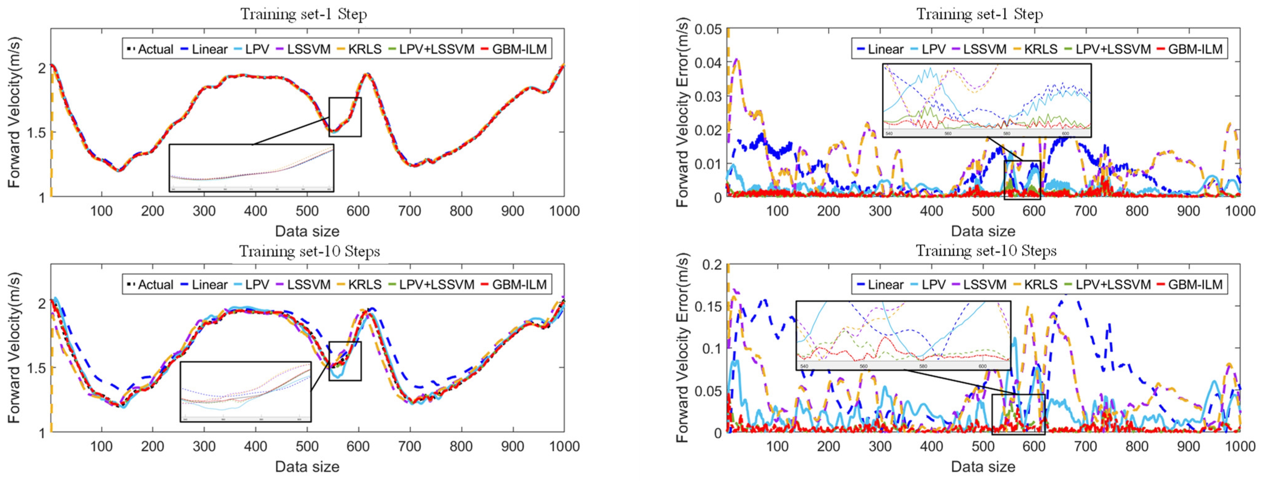
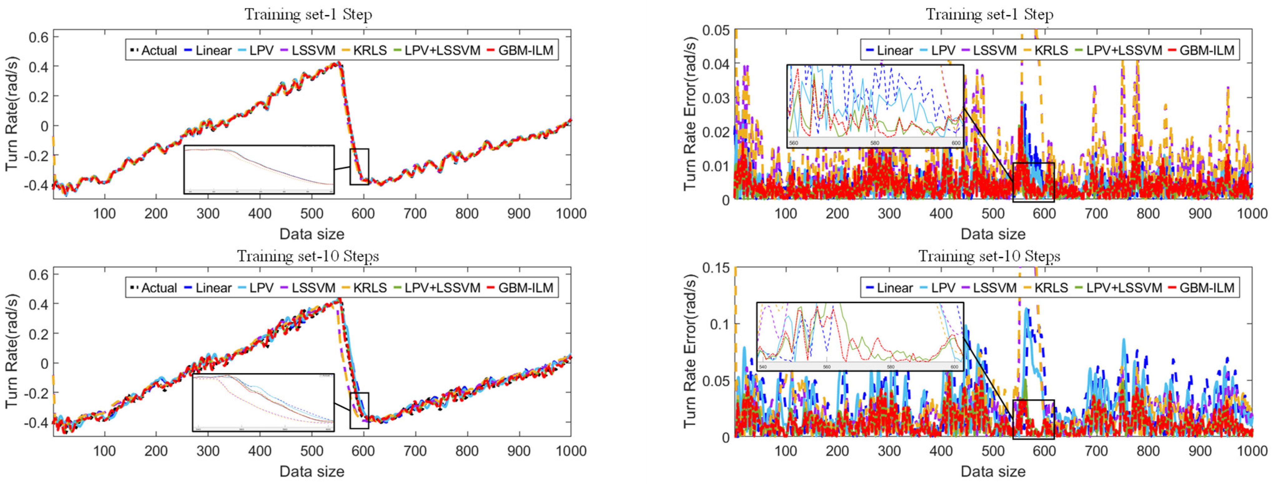
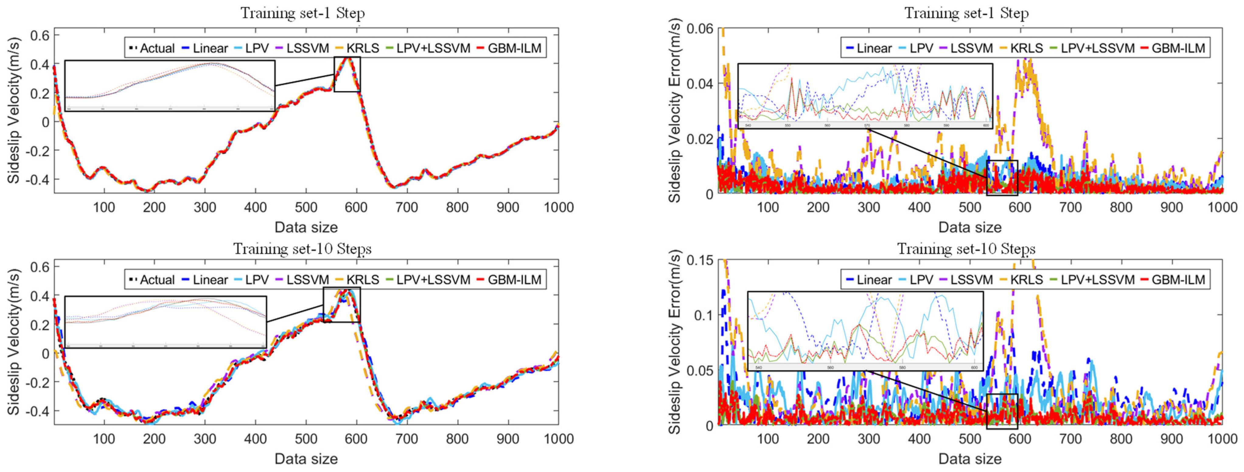
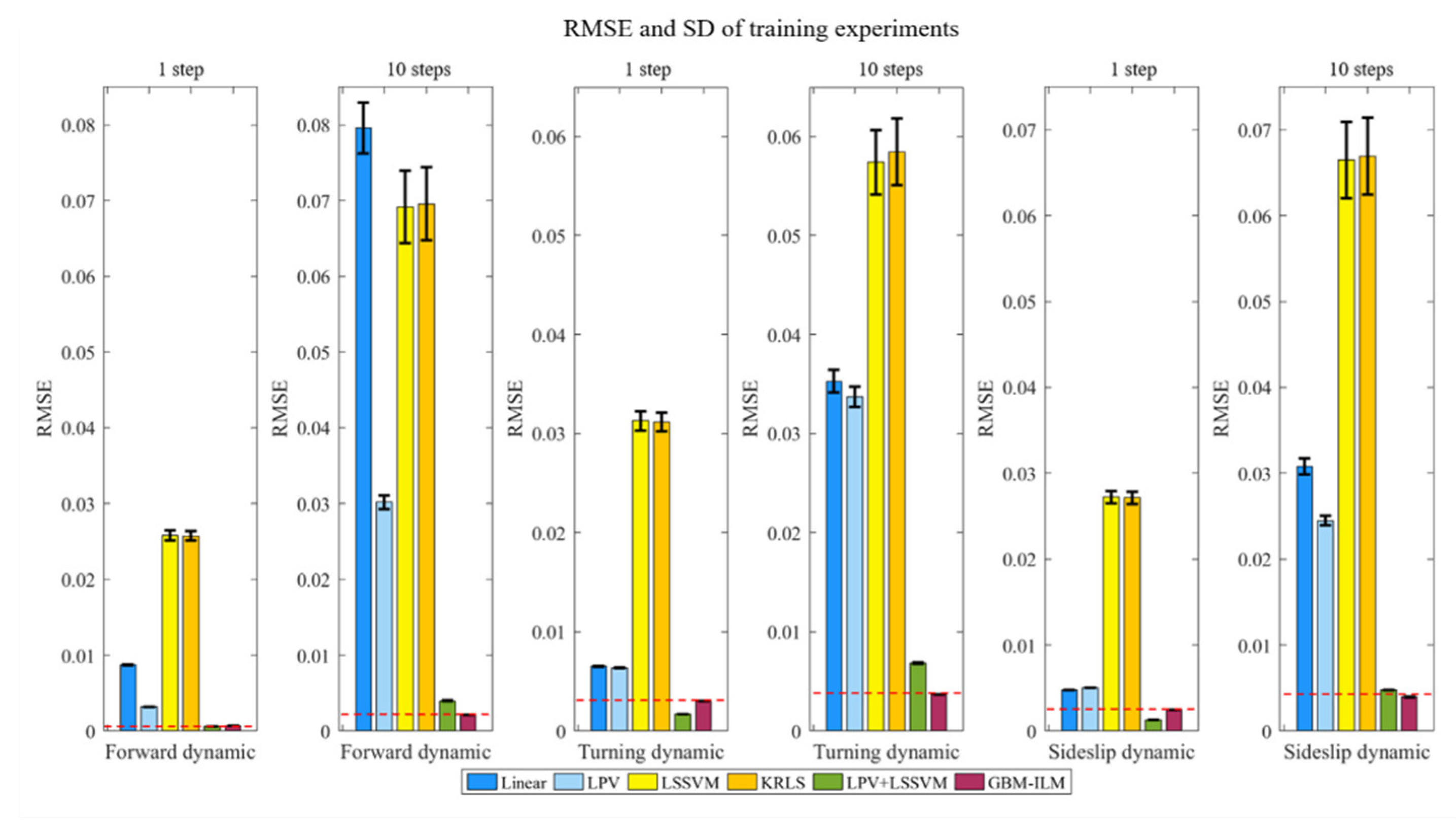
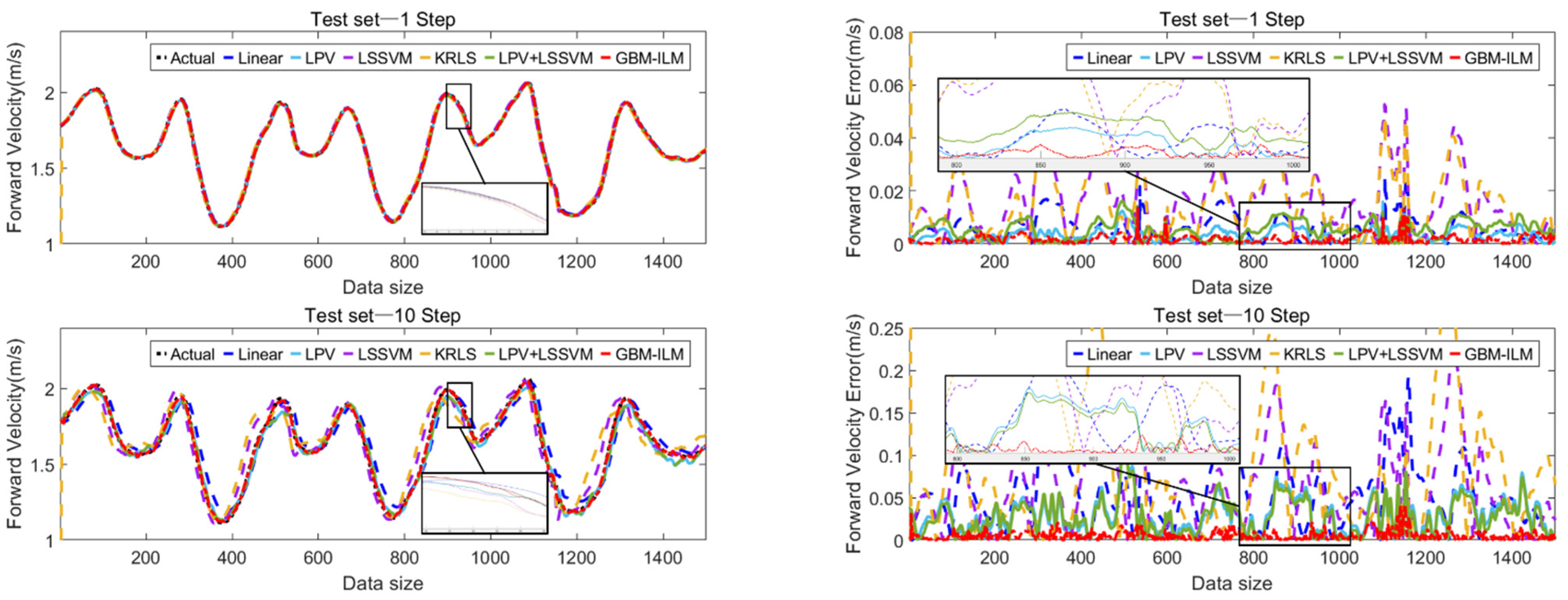
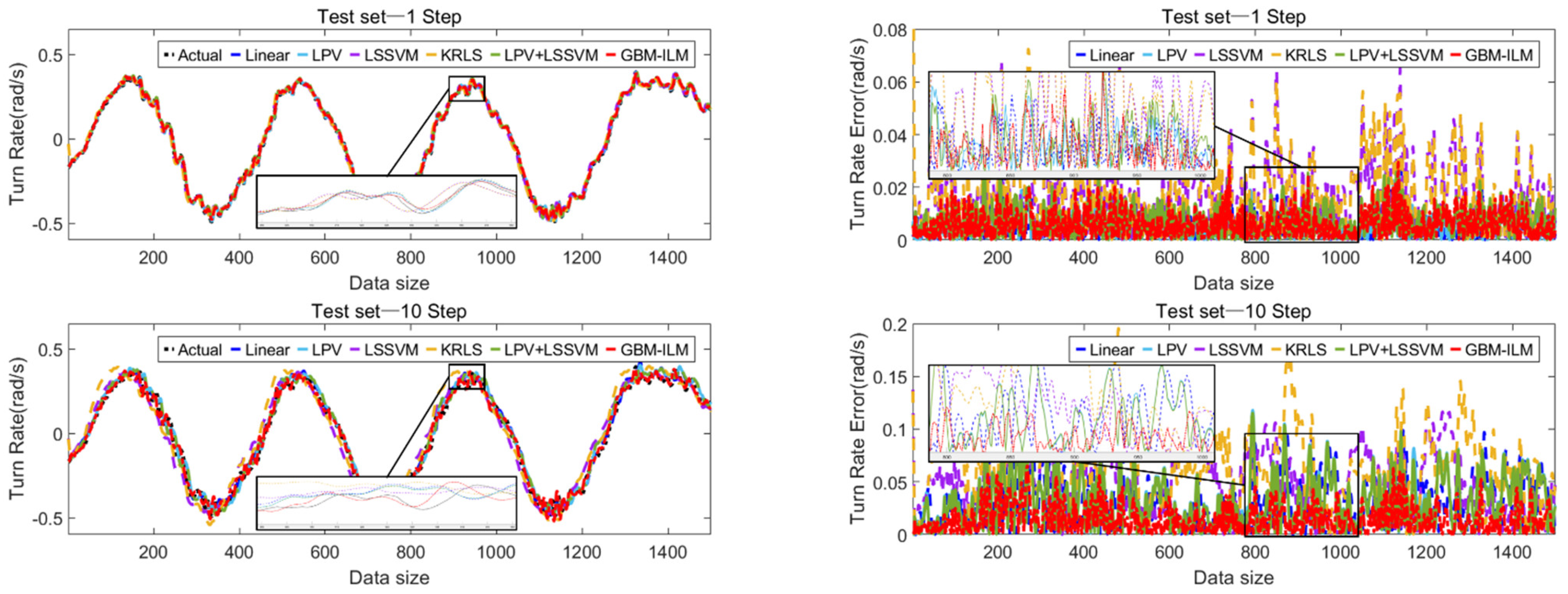
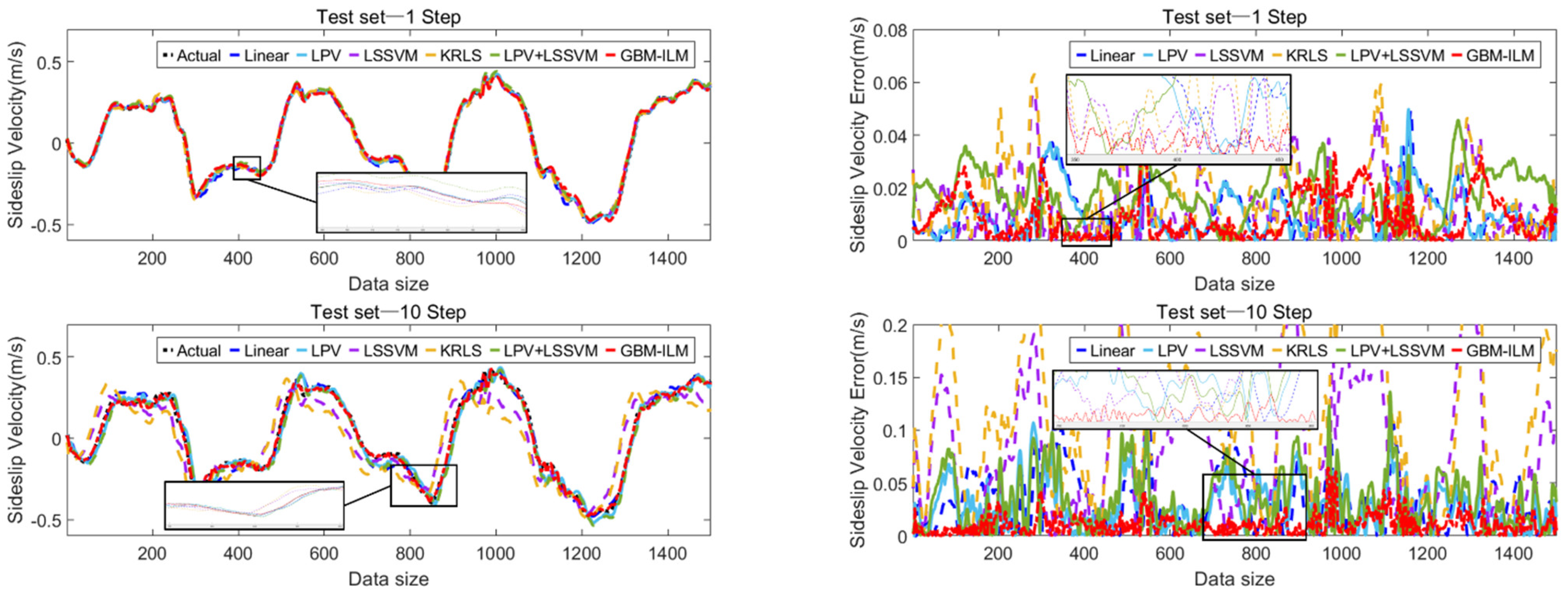
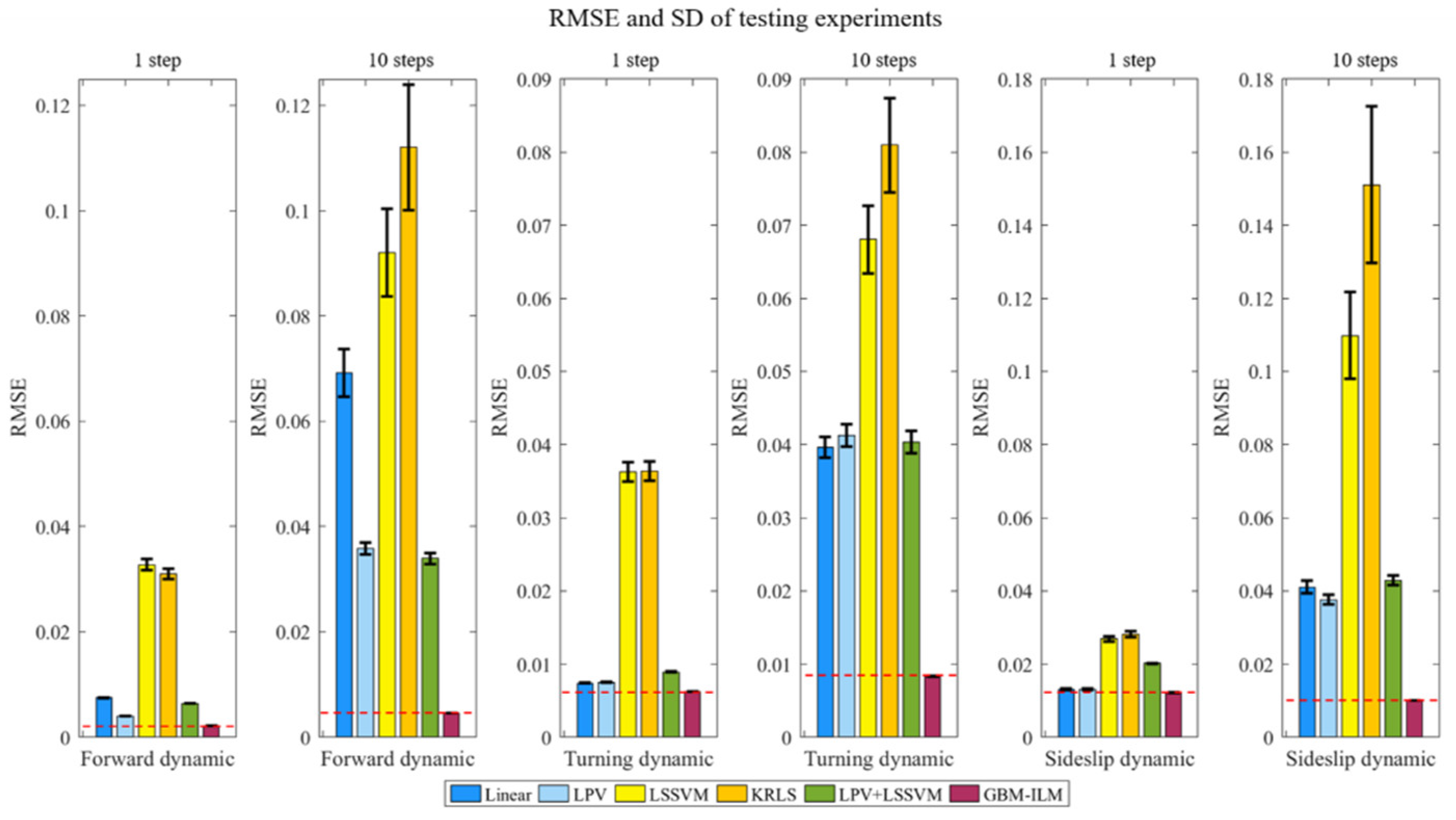
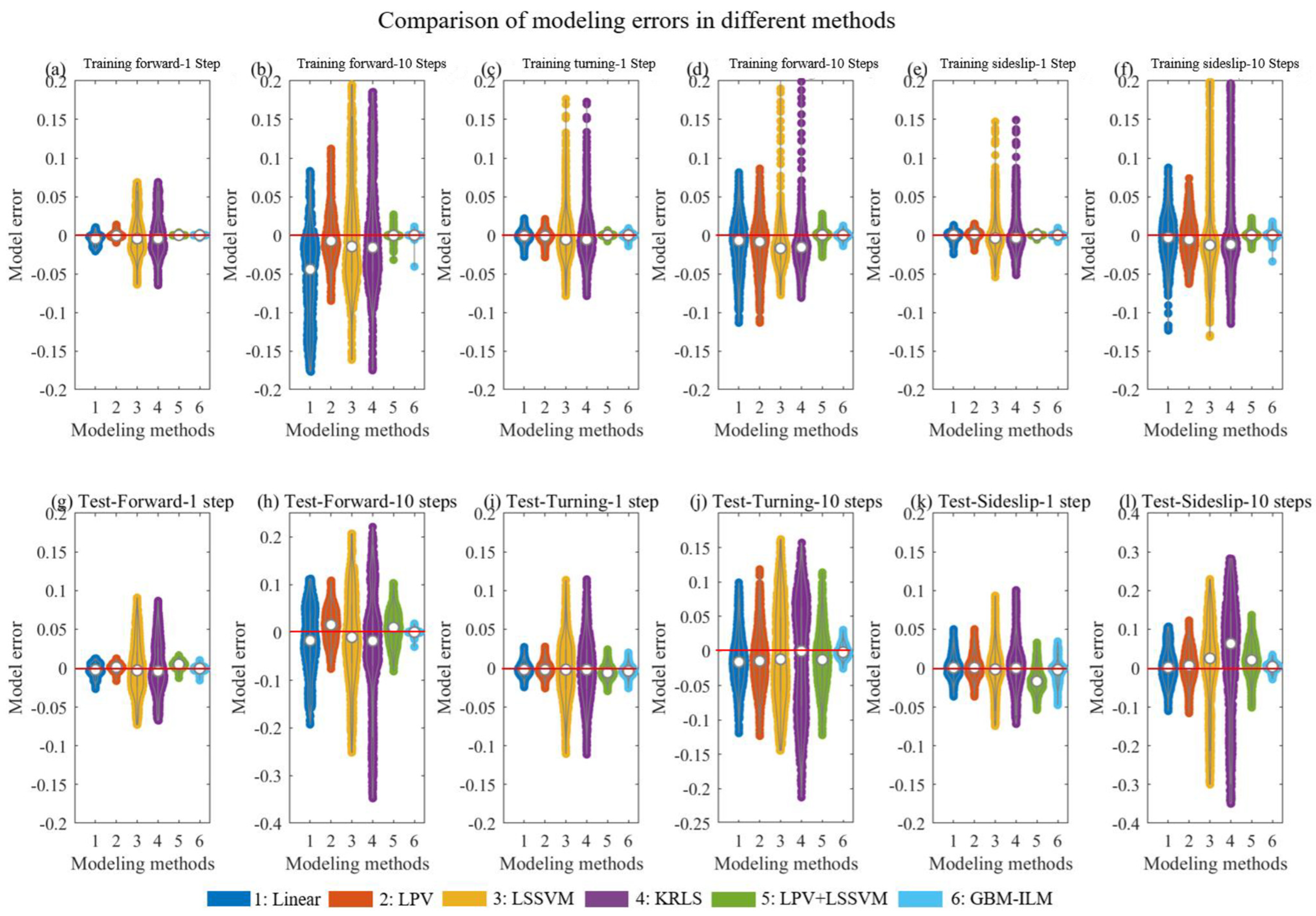
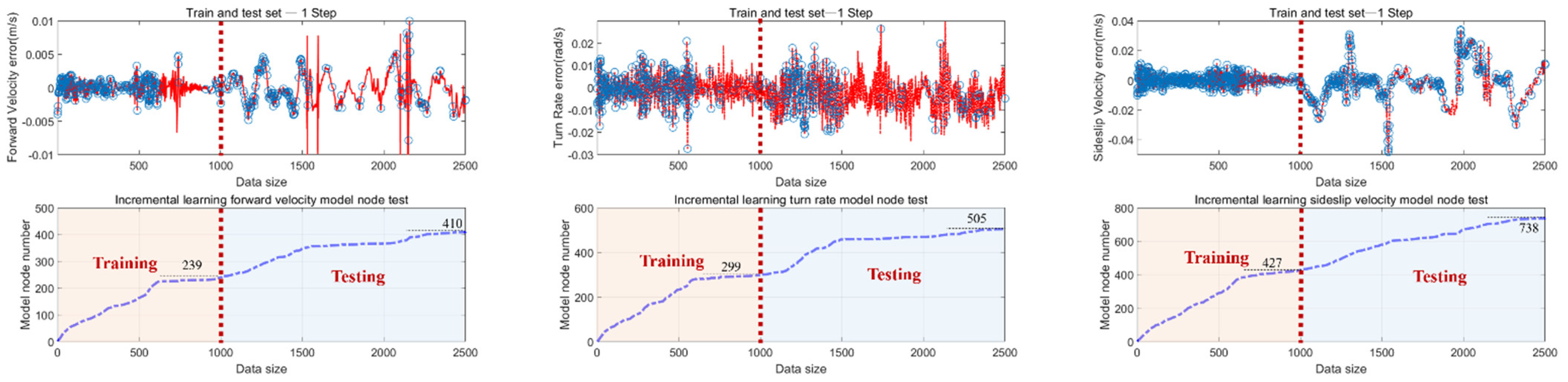
The efficacy of our resulting model was thoroughly evaluated through tests on a real USV system. For this, our research group developed a specialized ‘Salmon’ USV experimental platform and conducted identification tests in a reservoir under conditions classified as a sea state degree of two. Experimental data were meticulously selected for both the input and output data, enabling us to show the superior performance of our approach in predicting the kinetic model online, in comparison to other typical modeling methods. Compared to the LPV with LSSVM method (which performs best among the typical and state-of-the-art methods) from tests at 1-step, the GBM-ILM method improves by 46.34%, 14.86%, and 6.87% in accuracy when estimating the USV’s forward, turning, and sideslip dynamic models, respectively. The error ratios of the test data are 0.11%, 1.26%, and 3.05% of USV model states for the forward, turning, and sideslip dynamics, respectively.

Looking ahead, based on the GBM-ILM proposed in this study, the USV state after 0.5 s would be predicted under the premise of ensuring the model accuracy. Our future research will focus on the development of USV control systems.

References

1. Matsiko, A. Autonomous Boat Navigation in the Real World. Sci. Robot. 2023, 8, eadm9464. [Google Scholar] [CrossRef]
2. Bolbot, V.; Sandru, A.; Saarniniemi, T.; Puolakka, O.; Kujala, P.; Valdez Banda, O.A. Small Unmanned Surface Vessels—A Review and Critical Analysis of Relations to Safety and Safety Assurance of Larger Autonomous Ships. J. Mar. Sci. Eng. 2023, 11, 2387. [Google Scholar] [CrossRef]
3. Wang, W.; Fernández-Gutiérrez, D.; Doornbusch, R.; Jordan, J.; Shan, T.; Leoni, P.; Hagemann, N.; Schiphorst, J.K.; Duarte, F.; Ratti, C.; et al. Roboat III: An Autonomous Surface Vessel for Urban Transportation. J. Field Robot. 2023, 40, 1996–2009. [Google Scholar] [CrossRef]
4. Madeo, D.; Pozzebon, A.; Mocenni, C.; Bertoni, D. A Low-Cost Unmanned Surface Vehicle for Pervasive Water Quality Monitoring. IEEE Trans. Instrum. Meas. 2020, 69, 1433–1444. [Google Scholar] [CrossRef]
5. Zhang, M.; Li, D.; Xiong, J.; He, Y. Multi-Dimensional Water Sampling Unmanned Surface Vehicle Development and Application. Int. J. Dyn. Control 2023, 11, 3188–3208. [Google Scholar] [CrossRef]
6. Peng, Y.; Yang, Y.; Cui, J.; Li, X.; Pu, H.; Gu, J.; Xie, S.; Luo, J. Development of the USV ‘JingHai-I’ and Sea Trials in the Southern Yellow Sea. Ocean Eng. 2017, 131, 186–196. [Google Scholar] [CrossRef]
7. Huixi, X.; Chenglin, J. Heterogeneous Oceanographic Exploration System Based on USV and AUV:A Survey of Developments and Challenges. J. Univ. Chin. Acad. Sci. 2021, 38, 145–159. [Google Scholar]
8. Wang, Y.; Liu, W.; Liu, J.; Sun, C. Cooperative USV–UAV Marine Search and Rescue with Visual Navigation and Reinforcement Learning-Based Control. ISA Trans. 2023, 137, 222–235. [Google Scholar] [CrossRef] [PubMed]
9. Ouelmokhtar, H.; Benmoussa, Y.; Benazzouz, D.; Ait-Chikh, A.; Lemarchand, L. Energy-Based USV Maritime Monitoring Using Multi-Objective Evolutionary Algorithms. Ocean Eng. 2022, 253, 111182. [Google Scholar] [CrossRef]
10. Xie, J.; Zhou, R.; Luo, J.; Peng, Y.; Liu, Y.; Xie, S.; Pu, H. Hybrid Partition-Based Patrolling Scheme for Maritime Area Patrol with Multiple Cooperative Unmanned Surface Vehicles. J. Mar. Sci. Eng. 2020, 8, 936. [Google Scholar] [CrossRef]
11. Liu, Z.; Zhang, Y.; Yu, X.; Yuan, C. Unmanned Surface Vehicles: An Overview of Developments and Challenges. Annu. Rev. Control 2016, 41, 71–93. [Google Scholar] [CrossRef]
12. Sonnenburg, C.R.; Woolsey, C.A. Modeling, Identification, and Control of an Unmanned Surface Vehicle. J. Field Robot. 2013, 30, 371–398. [Google Scholar] [CrossRef]
13. Kahveci, N.E.; Ioannou, P.A. Adaptive Steering Control for Uncertain Ship Dynamics and Stability Analysis. Automatica 2013, 49, 685–697. [Google Scholar] [CrossRef]
14. Haranen, M.; Pakkanen, P.; Kariranta, R.; Salo, J. White, Grey and Black-Box Modelling in Ship Performance Evaluation; NAPA Ltd.: Helsinki, Finland, 2016. [Google Scholar]
15. Wang, X.; Zou, Z.; Yu, L.; Cai, W. System Identification Modeling of Ship Manoeuvring Motion in 4 Degrees of Freedom Based on Support Vector Machines. China Ocean Eng. 2015, 29, 519–534. [Google Scholar] [CrossRef]
16. Nomoto, K.; Taguchi, K.; Honda, K.; Hirano, S. On the Steering Qualities of Ships. J. Zosen Kiokai 1956, 1956, 75–82. [Google Scholar] [CrossRef] [PubMed]
17. Abkowitz, M.A. Lectures on Ship Hydrodynamics–Steering and Manoeuvrability; Report No. Hy-5, Lectures; Hydro- and Aerodynamics Laboratory, Hydrodynamics Section: Lyngby, Denmark, 1964. [Google Scholar]
18. Norrbin, N.H. Theory and Observations on the Use of a Mathematical Model for Ship Manoeuvring in Deep and Confined Waters. In Publication 68 of the Swedish State Shipbuilding Experimental Tank, Göteborg, Sweden, Proceedings of the 8th Symposium on Naval Hydrodynamics, ONR, Pasadena, CA, USA; 1971; pp. 807–905. Available online: https://repository.tudelft.nl/islandora/object/uuid:75736a6f-66e1-4c00-b3bc-897a19a232ea?collection=research (accessed on 14 March 2024).
19. Ogawa, A.; Kasai, H. On the mathematical model of manoeuvring motion of ships. Int. Shipbuild. Prog. 1978, 25, 306–319. [Google Scholar] [CrossRef]
20. Fossen, T.I. Nonlinear Modeling and Control of Underwater. Vehicles. Thesis, Universitetet i Trondheim, Trondheim, Norway, 1991. [Google Scholar]
21. Fossen, T. Handbook of Marine Craft Hydrodynamics and Motion Control; Wiley: Hoboken, NJ, USA, 2021. [Google Scholar] [CrossRef]
22. Yue, J.; Liu, L.; Gu, N.; Peng, Z.; Wang, D.; Dong, Y. Online Adaptive Parameter Identification of an Unmanned Surface Vehicle without Persistency of Excitation. Ocean Eng. 2022, 250, 110232. [Google Scholar] [CrossRef]
23. Wang, S.; Wang, L.; Im, N.; Zhang, W.; Li, X. Real-Time Parameter Identification of Ship Maneuvering Response Model Based on Nonlinear Gaussian Filter. Ocean Eng. 2022, 247, 110471. [Google Scholar] [CrossRef]
24. Perera, L.P.; Oliveira, P.; Guedes Soares, C. System Identification of Vessel Steering with Unstructured Uncertainties by Persistent Excitation Maneuvers. IEEE J. Ocean Eng. 2016, 41, 515–528. [Google Scholar] [CrossRef]
25. Alexandersson, M.; Mao, W.; Ringsberg, J.W. System Identification of Vessel Manoeuvring Models. Ocean Eng. 2022, 266, 112940. [Google Scholar] [CrossRef]
26. Revestido Herrero, E.; Velasco González, F.J. Two-Step Identification of Non-Linear Manoeuvring Models of Marine Vessels. Ocean Eng. 2012, 53, 72–82. [Google Scholar] [CrossRef]
27. Shen, H.; Wen, G.; Lv, Y.; Zhou, J.; Wang, L. USV Parameter Estimation: Adaptive Unscented Kalman Filter-Based Approach. IEEE Trans. Ind. Inf. 2022, 19, 7751–7761. [Google Scholar] [CrossRef]
28. Menges, D.; Rasheed, A. An Environmental Disturbance Observer Framework for Autonomous Surface Vessels. Ocean Eng. 2023, 285, 115412. [Google Scholar] [CrossRef]
29. Zhang, G.; Zhang, X.; Pang, H. Multi-Innovation Auto-Constructed Least Squares Identification for 4 DOF Ship Manoeuvring Modelling with Full-Scale Trial Data. ISA Trans. 2015, 58, 186–195. [Google Scholar] [CrossRef] [PubMed]
30. Xu, H.; Hassani, V.; Guedes Soares, C. Uncertainty Analysis of the Hydrodynamic Coefficients Estimation of a Nonlinear Manoeuvring Model Based on Planar Motion Mechanism Tests. Ocean Eng. 2019, 173, 450–459. [Google Scholar] [CrossRef]
31. Xiong, Y.; Wang, X.; Pan, L.; Zhou, S. Research on Online Interactive Identification Method for Motion Model of Double Propeller Propulsion Unmanned Surface Vehicle Based on ESO Disturbance Estimation. Ocean Eng. 2023, 285, 115328. [Google Scholar] [CrossRef]
32. Zhang, D.; Chu, X.; Wu, W.; He, Z.; Wang, Z.; Liu, C. Model Identification of Ship Turning Maneuver and Extreme Short-Term Trajectory Prediction under the Influence of Sea Currents. Ocean Eng. 2023, 278, 114367. [Google Scholar] [CrossRef]
33. Wang, Z.; Zou, Z.; Guedes Soares, C. Identification of Ship Manoeuvring Motion Based on Nu-Support Vector Machine. Ocean Eng. 2019, 183, 270–281. [Google Scholar] [CrossRef]
34. Zhang, Y.-Y.; Wang, Z.-H.; Zou, Z.-J. Black-Box Modeling of Ship Maneuvering Motion Based on Multi-Output Nu-Support Vector Regression with Random Excitation Signal. Ocean Eng. 2022, 257, 111279. [Google Scholar] [CrossRef]
35. Pan, C.-Z.; Lai, X.-Z.; Yang, S.X.; Wu, M. An Efficient Neural Network Approach to Tracking Control of an Autonomous Surface Vehicle with Unknown Dynamics. Expert Syst. Appl. 2013, 40, 1629–1635. [Google Scholar] [CrossRef]
36. Xu, W.; Maki, K.J.; Silva, K.M. A Data-Driven Model for Nonlinear Marine Dynamics. Ocean Eng. 2021, 236, 109469. [Google Scholar] [CrossRef]
37. Skulstad, R.; Li, G.; Fossen, T.I.; Vik, B.; Zhang, H. A Hybrid Approach to Motion Prediction for Ship Docking—Integration of a Neural Network Model Into the Ship Dynamic Model. IEEE Trans. Instrum. Meas. 2021, 70, 2501311. [Google Scholar] [CrossRef]
38. Zhang, X.-G.; Zou, Z.-J. Black-Box Modeling of Ship Manoeuvring Motion Based on Feed-Forward Neural Network with Chebyshev Orthogonal Basis Function. J. Mar. Sci. Technol. 2013, 18, 42–49. [Google Scholar] [CrossRef]
39. Wang, N.; Er, M.J.; Han, M. Large Tanker Motion Model Identification Using Generalized Ellipsoidal Basis Function-Based Fuzzy Neural Networks. IEEE Trans. Cybern. 2015, 45, 2732–2743. [Google Scholar] [CrossRef]
40. Dimitrov, M.; Groves, K.; Howard, D.; Lennox, B. Model Identification of a Small Fully-Actuated Aquatic Surface Vehicle Using a Long Short-Term Memory Neural Network. In Proceedings of the 2021 IEEE International Conference on Robotics and Automation (ICRA), Xi’an, China, 30 May–5 June 2021; pp. 5966–5972. [Google Scholar]
41. He, H.-W.; Wang, Z.-H.; Zou, Z.-J.; Liu, Y. Nonparametric Modeling of Ship Maneuvering Motion Based on Self-Designed Fully Connected Neural Network. Ocean Eng. 2022, 251, 111113. [Google Scholar] [CrossRef]
42. Woo, J.; Park, J.; Yu, C.; Kim, N. Dynamic Model Identification of Unmanned Surface Vehicles Using Deep Learning Network. Appl. Ocean Res. 2018, 78, 123–133. [Google Scholar] [CrossRef]
43. Sjöberg, J.; Zhang, Q.; Ljung, L.; Benveniste, A.; Delyon, B.; Glorennec, P.-Y.; Hjalmarsson, H.; Juditsky, A. Nonlinear Black-Box Modeling in System Identification: A Unified Overview. Automatica 1995, 31, 1691–1724. [Google Scholar] [CrossRef]
44. Luo, W.; Moreira, L.; Guedes Soares, C. Manoeuvring Simulation of Catamaran by Using Implicit Models Based on Support Vector Machines. Ocean Eng. 2014, 82, 150–159. [Google Scholar] [CrossRef]
45. Wang, Z.; Xu, H.; Xia, L.; Zou, Z.; Soares, C.G. Kernel-Based Support Vector Regression for Nonparametric Modeling of Ship Maneuvering Motion. Ocean Eng. 2020, 216, 107994. [Google Scholar] [CrossRef]
46. Xue, Y.; Liu, Y.; Ji, C.; Xue, G. Hydrodynamic Parameter Identification for Ship Manoeuvring Mathematical Models Using a Bayesian Approach. Ocean Eng. 2020, 195, 106612. [Google Scholar] [CrossRef]
47. Suykens, J.A.K.; Vandewalle, J. Least Squares Support Vector Machine Classifiers. Neural Process. Lett. 1999, 9, 293–300. [Google Scholar] [CrossRef]
48. Xu, H.; Guedes Soares, C. Vector Field Path Following for Surface Marine Vessel and Parameter Identification Based on LS-SVM. Ocean Eng. 2016, 113, 151–161. [Google Scholar] [CrossRef]
49. Zhu, M.; Sun, W.; Hahn, A.; Wen, Y.; Xiao, C.; Tao, W. Adaptive Modeling of Maritime Autonomous Surface Ships with Uncertainty Using a Weighted LS-SVR Robust to Outliers. Ocean Eng. 2020, 200, 107053. [Google Scholar] [CrossRef]
50. Xu, H.; Guedes Soares, C. Manoeuvring Modelling of a Containership in Shallow Water Based on Optimal Truncated Nonlinear Kernel-Based Least Square Support Vector Machine and Quantum-Inspired Evolutionary Algorithm. Ocean Eng. 2020, 195, 106676. [Google Scholar] [CrossRef]
51. Xu, H.; Hinostroza, M.A.; Hassani, V.; Guedes Soares, C. Real-Time Parameter Estimation of a Nonlinear Vessel Steering Model Using a Support Vector Machine. J. Offshore Mech. Arct. Eng. 2019, 141, 061606. [Google Scholar] [CrossRef]
52. Xu, P.-F.; Cheng, C.; Cheng, H.-X.; Shen, Y.-L.; Ding, Y.-X. Identification-Based 3 DOF Model of Unmanned Surface Vehicle Using Support Vector Machines Enhanced by Cuckoo Search Algorithm. Ocean Eng. 2020, 197, 106898. [Google Scholar] [CrossRef]
53. Ariza Ramirez, W.; Leong, Z.Q.; Nguyen, H.; Jayasinghe, S.G. Non-Parametric Dynamic System Identification of Ships Using Multi-Output Gaussian Processes. Ocean Eng. 2018, 166, 26–36. [Google Scholar] [CrossRef]
54. Astfalck, L.C.; Cripps, E.J.; Hodkiewicz, M.R.; Milne, I.A. A Bayesian Approach to the Quantification of Extremal Responses in Simulated Dynamic Structures. Ocean Eng. 2019, 182, 594–607. [Google Scholar] [CrossRef]
55. Xue, Y.; Liu, Y.; Ji, C.; Xue, G.; Huang, S. System Identification of Ship Dynamic Model Based on Gaussian Process Regression with Input Noise. Ocean Eng. 2020, 216, 107862. [Google Scholar] [CrossRef]
56. Xue, Y.; Chen, G.; Li, Z.; Xue, G.; Wang, W.; Liu, Y. Online Identification of a Ship Maneuvering Model Using a Fast Noisy Input Gaussian Process. Ocean Eng. 2022, 250, 110704. [Google Scholar] [CrossRef]
57. Ouyang, Z.-L.; Zou, Z.-J. Nonparametric Modeling of Ship Maneuvering Motion Based on Gaussian Process Regression Optimized by Genetic Algorithm. Ocean Eng. 2021, 238, 109699. [Google Scholar] [CrossRef]
58. Liu, S.-Y.; Ouyang, Z.-L.; Chen, G.; Zhou, X.; Zou, Z.-J. Black-Box Modeling of Ship Maneuvering Motion Based on Gaussian Process Regression with Wavelet Threshold Denoising. Ocean Eng. 2023, 271, 113765. [Google Scholar] [CrossRef]
59. Hewing, L.; Wabersich, K.P.; Menner, M.; Zeilinger, M.N. Learning-Based Model Predictive Control: Toward Safe Learning in Control. Annu. Rev. Control Robot. Auton. Syst. 2020, 3, 269–296. [Google Scholar] [CrossRef]
60. Mei, B.; Sun, L.; Shi, G. White-Black-Box Hybrid Model Identification Based on RM-RF for Ship Maneuvering. IEEE Access 2019, 7, 57691–57705. [Google Scholar] [CrossRef]
61. Chen, L.; Yang, P.; Li, S.; Tian, Y.; Liu, G.; Hao, G. Grey-Box Identification Modeling of Ship Maneuvering Motion Based on LS-SVM. Ocean Eng. 2022, 266, 112957. [Google Scholar] [CrossRef]
62. Han, J.; Xiong, J.; He, Y.Q.; Gu, F.; Li, D. Nonlinear Modeling for a Water-Jet Propulsion USV: An Experimental Study. IEEE Trans. Ind. Electron. 2016, 64, 3348–3358. [Google Scholar] [CrossRef]
63. Engel, Y.; Mannor, S.; Meir, R. The Kernel Recursive Least-Squares Algorithm. IEEE Trans. Signal Process. 2004, 52, 2275–2285. [Google Scholar] [CrossRef]
64. Hu, Y.; Li, D.; He, Y.; Han, J. Q-Learning Algorithm Based on Incremental RBF Network. Robot 2019, 41, 562–573. [Google Scholar] [CrossRef]
65. Sonnenburg, C.; Gadre, A.; Horner, D.; Kragelund, S.; Marcus, A.; Stilwell, D.J.; Woolsey, C.A. Control-Oriented Planar Motion Modeling of Unmanned Surface Vehicles. In Proceedings of the OCEANS 2010 MTS/IEEE SEATTLE, Seattle, WA, USA, 20–23 September 2010; pp. 1–10. [Google Scholar]
66. Xiong, J.; He, Y.; Han, J. Active LPV Yaw Keeping Control of an Unmanned Surface Vehicle. Inf. Control 2018, 47, 267–275+282. [Google Scholar] [CrossRef]
67. Raïssi, T.; Videau, G.; Zolghadri, A. Interval Observer Design for Consistency Checks of Nonlinear Continuous-Time Systems. Automatica 2010, 46, 518–527. [Google Scholar] [CrossRef]
68. Balakrishnan, V. System Identification: Theory for the User (Second Edition): Lennart Ljung; Prentice-Hall, Englewood Cliffs, NJ, 1999, ISBN 0-13-656695-2. Automatica 2002, 38, 375–378. [Google Scholar] [CrossRef]
69. Shi, X.; Xiong, W. Approximate Linear Dependence Criteria with Active Learning for Smart Soft Sensor Design. Chemom. Intell. Lab. Syst. 2018, 180, 88–95. [Google Scholar] [CrossRef]
70. Datta, K. Linear System Theory and Design, by Chi-Tsong Chen. Int. J. Robust Nonlinear Control 2000, 10, 1360–1362. [Google Scholar]
Figure 1. System dynamics modeling classification.
Jmse 12 00627 g001
Figure 2. Flow graph of the GBM-ILM method.
Jmse 12 00627 g002
Figure 3. Coordinate frames for the USV, where ( X i , Y i , E ) is the inertial coordinate frame, ( X b , Y b , O ) is the USV body coordinate frame, V is the USV’s resultant velocity. The nomenclature of main parameters is listed in Table 2, as is the nomenclature used below.
Jmse 12 00627 g003
Figure 4. Model error prediction flow based on KRLS-ALD network.
Jmse 12 00627 g004
Figure 5. USV experimental platform and hardware system.
Jmse 12 00627 g005
Figure 6. Electric and communication flow of ‘Salmon’ USV.
Jmse 12 00627 g006
Figure 7. Software structure of the USV.
Jmse 12 00627 g007
Figure 8. USV identification experiments.
Jmse 12 00627 g008
Figure 9. USV identification experiments data results. (a) Linear experiment; (b) zigzag experiment ( ε = 30 % ).
Jmse 12 00627 g009
Figure 10. Crosscheck experiments for GBM-ILM. (a) Forward dynamic; (b) turning dynamic; (c) sideslip dynamic.
Jmse 12 00627 g010
Figure 11. Comparisons of forward velocity model and forward velocity error.
Jmse 12 00627 g011
Figure 12. Comparisons of turning rate model and turning rate error.
Jmse 12 00627 g012
Figure 13. Comparisons of sideslip velocity model and sideslip velocity error.
Jmse 12 00627 g013
Figure 14. RMSE and SD of training experiments.
Jmse 12 00627 g014
Figure 15. Comparisons of forward velocity model and forward velocity error.
Jmse 12 00627 g015
Figure 16. Comparisons of turning rate model and turning rate error.
Jmse 12 00627 g016
Figure 17. Comparisons of sideslip velocity model and sideslip velocity error.
Jmse 12 00627 g017
Figure 18. RMSE and SD of testing experiments.
Jmse 12 00627 g018
Figure 19. Comparison of modeling error in different methods.
Jmse 12 00627 g019
Figure 20. Incremental learning model node update process.
Jmse 12 00627 g020