Sub-Bottom Sediment Classification Employing a Multi-Attribute Temporal Convolutional Network

Abstract

Sub-bottom profile data have the potential to characterize sediment properties but are seldom used for offshore site investigations because of uncertainties in rock-physics models. Deep-learning techniques appear to be poised to play very important roles in our processing flows for the interpretation of geophysical data. In this paper, a novel deep learning-based method for this task is proposed in which a nonlinear mapping between the observed data and sediment types is learned using a multi-attribute temporal convolution network (MATCN). Firstly, empirical mode decomposition (EMD) is employed for the original data, and intrinsic mode functions (IMFs) with multiple time scales are generated. Based on different IMFs, instantaneous frequency (IF) data under different IMFs can be obtained, while instantaneous phase (IP) and instantaneous amplitude (IA) data are obtained based on the original data. IF, IA and IP data are called attribute data, and are highly related to the attenuation, reflection, and interior structure of the sediment. Thus, IA, IF, and IP are used as the inputs, and a 1D convolutional neural network (CNN) and a time convolution network (TCN) are used to extract sequential features. Different feature representations are then fused. Combining cross-entropy loss function and class-edge loss function, the network is encouraged to produce classified results with more continuous sediment distributions compared with the traditional loss function. The real-data experiments demonstrate that the proposed MATCN has achieved good performance with an F measure greater than 70% in all cases, and greater than 80% in most cases.

1. Introduction

A sub-bottom profiler (SBP) is designed to image underwater sub-bottom sediment for waterway dredging, marine scientific research, etc. [1,2,3,4,5,6,7]. Nowadays, SBP imaging is widely used as a tool with which to map and interpret changes in sub-bottom reservoirs. However, the existing use of sub-bottom profilers has remained limited mostly to the delineation of sub-bottom layers, though remote acoustic classification of the physical properties of sub-bottom sediments is of paramount interest to the geotechnical and geological communities [1,2,3,4,5]. Sediment types are still difficult to discern because of uncertainties in rock-physics models [7]. To manage this problem and improve the classification ability of SBP data, many researchers are conducting studies in this field through different methods.

Some researchers have attempted to classify the sub-bottom sediment based on the attribute of the reflection coefficient (RC), as the RC is highly related to acoustic impedance [8,9]. In fact, sediment classification methods based on the RC are also very simple and efficient. The first approach, building on Mohamed’s work [8], focuses on calculating the RC by utilizing the energy of signals reflected from diverse interfaces. This involves formulating an equation that describes the acoustic energy across multiple layers in order to determine the RC for each sediment layer interface. Similarly, Plets [9] adopted the RC as a straightforward and effective means by which to examine the characteristics of sub-bottom properties. The RC was determined by taking the ratio of the reflected wave’s amplitude to that of the incident wave. Despite these developments, sub-bottom applications face challenges when acquiring reflection coefficients due to the limitations in existing methods; for example, Mohamed’s method is contingent upon an optimal window size parameter, which is difficult to ascertain, and Plets’ approach may not be applicable if multiplicity is absent.

As the reflection coefficient-based method always needs the help of multiple reflections, it can be invalid when no multiple reflection exists. Because the higher frequencies are used, as in the case of shallow sub-bottom profiling, attenuation significantly alters the reflection response. Thus, the attenuation parameter is rather important for SBP classification. Initially, the spectral ratio technique, as documented in [10,11], was modified for use with seismic-reflection data, enabling the direct quantification of compression wave attenuation in terms of two-way travel time, rather than relying on distance and velocity metrics. Furthermore, Panda [12] constructed an attenuation-based classification model that correlates the relaxation time of sediments with changes in the instantaneous frequency of acoustic signals. Stevenson et al. [13] refined LeBlanc’s approach by determining instantaneous frequency alterations exclusively from the analysis of maximum envelope values.

The above methods all used the Hilbert transform to extract instantaneous frequency information from Chirp sonar, which has a high time resolution. However, IF is usually highly polluted by noise, and it is hard to obtain the trend of the shift in instantaneous frequency [14,15,16]. Pinson et al. [17] proposed a method by which to obtain quality factor Q by fitting a curve through iterative regression using the weighted robust least-squares method. However, the method is more suitable for estimating the physical properties of sediments between two parallel adjacent interfaces. In conclusion, methods based on IF and IA data are highly related to physical properties but are not suitable for the classification of all survey lines because of the limitations associated with noise sensitive and model conditions. Recently, Li et al. [18] have proposed a reflection signal decomposition method to obtain better acoustic attenuation parameters for sub-bottom sediment classification, which decomposes the overlapping reflection into separate reflection sub-signals to avoid spectrum vibration.

The above methods are based on acoustic attributes; however, they are limited to these acoustic attributes and a single attribute can hardly reflect well the features of the sediment. To this end, machine learning and feature engineering methods have been applied in the field of geophysics to widen the use of features used to classify the sediment. These methods can find potential relative relationships between the observed data and the material properties. Yegireddi et al. [19] have proposed a sediment classification method based on SBP image texture features. Texture can reflect the attributes of sediment characteristics to some degree; however, the relationship between texture features and sediment properties is not significant. Additionally, the classified results are based on patches, thus the resolution of the result is relatively low. A similarity index feature has been proposed by Gwang et.al [20]. The authors introduced the similarity index (SI) for the classification of the sea floor from acoustic profiling data. They found that various sediments can result in distinct waveform characteristics in neighboring received signals, with the SI serving as a measure for the similarity among these signals. The SI is employed in order to classify seafloor types but is considered unsuitable for categorizing sub-bottom sediments. Recently, Zong et al. [21] proposed a novel method based on variational mode decomposition (VMD) and texture features clustering to classify the sediment, but this method is time consuming.

On account of its powerful feature extraction and expression abilities, deep learning has been applied to many fields [22,23,24,25,26,27,28], as it shows better feature extraction ability than traditional machine learning methods. For sediment classification tasks, several solutions have been provided that utilize data-driven learning frameworks. Das et al. [29] used a 1D convolutional neural network (CNN) to obtain the impedance of seismic data. Wang et al. [30] used a fully convolutional residual network for seismic impedance inversion, as this can effectively predict impedance with high accuracy and it has good robustness. Li et al. [31] exploited a CNN to generate a model for full wave inversion optimization. Wang et al. [32,33] proposed a seismic inversion method based on a convolutional neural network with a physical constraint. To obtain better lateral continuity of the results, a two-dimensional bilateral filtering method was also adopted in their work. Di and Abubakar [34] adopted a semi-supervised learning framework, into which they introduced their logging data, in order to estimate acoustic impedance based on 3D seismic data. The above works show that the deep learning method is data-driven and shows great potential to get good results.

Deep learning-based methods are robust and can explore underlying relationships between observed data and physical sediment properties from abundant data. They also have great potential to obtain the potential relationship between observed data and the sediment. The traditional method using IF and IA data can also reveal the physical properties of sub-bottom sediments.

To this end, we proposed a sediment classes prediction method combining a deep learning network and which took instantaneous attributes into consideration in order to address the problems that traditional methods have encountered in terms of noise-sensitive data condition limits. An MATCN was proposed for sediment classification considering the IA, IF, and IP data classification potentials, which fuse multiple attributes to explore the latent sediment characteristics. MATCN is constructed by combining 1D CNN with TCN to better achieve feature extraction. Then the multiple attributes are put into the deep learning model to predict the sediment types. The paper is organized as follows. In Section 2 the proposed method is described. The experimental results and discussions are presented in Section 3 and Section 4. Finally, our conclusions are given in Section 5. 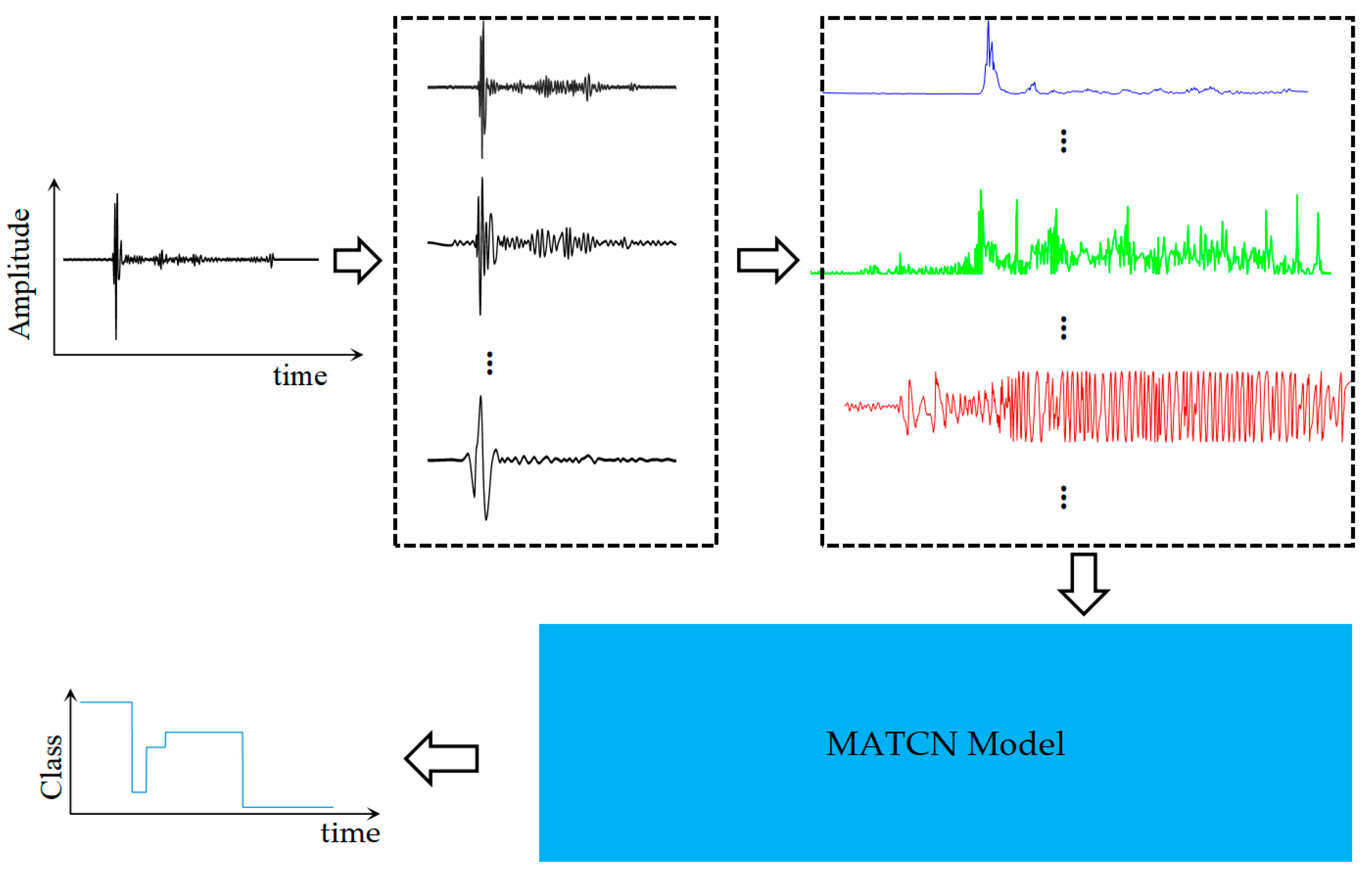The flowchart is shown in Figure 1.

2. Methods

2.1. Multi-Attribute Inputs

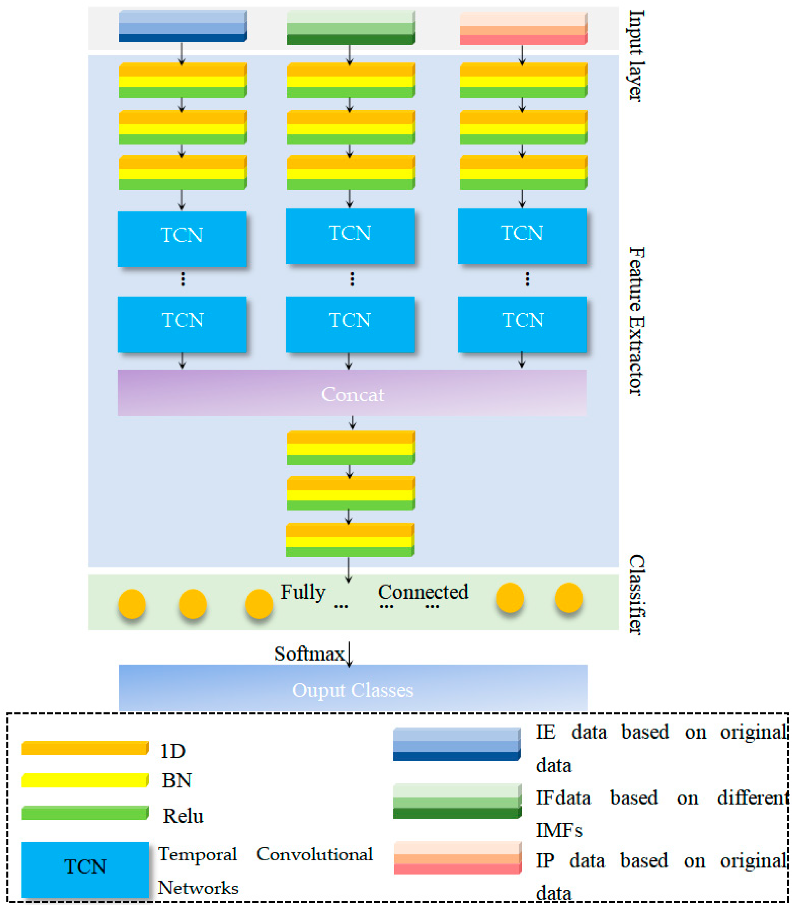
Through the learning of a time convolutional network, using instantaneous attributes as inputs, we present an MATCN model for sub-bottom sediment classification. The MATCN model simultaneously uses IA, IF, and IP data [35,36,37,38,39] as inputs and outputs the classified result. The flowchart of the classification with the MATCN model is depicted in Figure 2.

As shown in Figure 1. At first, the original received echo data is processed using EMD [40]. Then, a set of IMFs can be obtained. Based on the IMFs, the IA, IP, and IF series are generated. Concatenating IAs of different IMFs, the input IA block is built. The input IF and IP blocks can be generated in the same manner. The input blocks are subsequently fed into the feature extraction model. Convolution layers, as well as TCN blocks, constitute the feature extraction model and extract useful features under different time scales, which expand the ability to obtain different information [41,42].

Figure 2 illustrates the architecture of the proposed MATCN model. The top-left corner represents the input IA data of size L × N, while the top-median and top-right corner represent the input IF and IP data of size L × N, respectively. The 1D convolution layers follow behind the inputs. After 1D convolution, the TCN networks are used to extract the temporal characteristics. Then, by concatenating the extracted feature maps of three different inputs, the result is put into another 1D convolution network. A fully connected layer is used as the classifier. All of the convolution layers employ 1 × 3 convolution kernels with a stride equaling 1.

One distinct advantage of this joint instantaneous multi-attribute learning strategy is that the proposed method explores the potential nonlinear relationship between the attributes and the sediment types. The proposed MATCN employs edge loss and cross-entropy loss functions to optimize the model’s trainable parameters to obtain better results.

2.2. Multi-Attribute Inputs

Multi-Attribute Calculation

Instantaneous attributes have been widely used in seismic data analysis. Since sub-bottom data is a form of high-resolution seismic data, instantaneous attributes have also been introduced into sub-bottom data analysis. The instantaneous frequency has a high relationship with the sediment types. Thus, many sediment property estimation methods have been developed based on IF information. IF data is highly related to the attenuation features of the sediment layers.

Except for the IF, which is highly related to the types of the sub-bottom sediment types, the IA and IP are also important. The energy data, which is derived from the IA data, can be used to estimate the reflection coefficients. The received and transmitted energy ratio accounts for energy propagation and its corresponding geometrical and sediment attenuation losses. The sub-bottom acoustic energy propagation model is also built based on the IA data, which is highly related to the reflection attributes of the sediment properties.

IP data can describe the interior structure of sediment layers. In low- and moderate-loss dielectric media, the propagated acoustic signal shows significant changes in its amplitude spectrum, whereas the phase spectrum changes are regardless. Thus, the IP data can highlight all of the reflections regardless of the changes of amplitude. Consequently, the details of interior reflections with low amplitude can be well obtained. In conclusion, IP data can describe the morphological characters of sediment layers.

Usually, Hilbert transformation is used to obtain analytic signals and instantaneous attributes. However, to obtain IF data, one must obtain the derivation of IF, which is not robust to the noise. In fact, over several decades, researchers have been attempting to exploit the concept of IF derived from analytic signals to construct a robust time–frequency representation. However, the past applications of the Hilbert transform have been limited to the narrow band-passed signal. This was so until 1998, when Huang proposed a new method based on the Hilbert transformation, the key idea of which is the EMD [40]. The basic approach of the EMD method is to decompose a signal into a collection of intrinsic IMF that allows well-behaved Hilbert transforms for the computation of instantaneous frequencies that have physical means. Each IMF contains the local characteristic signal of the original signal in different time scales. Thus, employing the EMD calculation, a set of IMFs that can reflect the multi-time scale characteristics of the original signal can be obtained. IA, IF, and IP data can be obtained which can reflect the multiple time-scale characteristics of the original signal.

At first the EMD is applied [40].

x(t) is the original signal.

Step 1. Initialization, r₁(t) = x(t), i = 1, k = 0;

Step 2. Obtain the nth IMF

(a) Initialization, h₁(t) = r₁(t)

(b) Find the maximum and minimum of h_k(t)

(c) Use cubic spline interpolation to fit the maximum and minimum in order to obtain the upper and lower envelope e₊(t) and e₋(t);

(d) Obtain the mean of envelope m_k(t);

(e) h_k+1(t) = h_k(t) − m_k(t);

(f) Judge $SD=\frac{{\displaystyle \sum {\left[h_k(t)-h_{k-1}(t)\right]}^2}}{{\displaystyle \sum {\left[h_{k-1}(t)\right]}^2}}$;

Step 3. r_k+1(t) = r_k(t) − c_k+1(t), judge if the residual is constant or monotonic. If yes, EMD is ended and c_k(t) is the IMF. Every IMF is treated as a real part of the complex signal, and the imaginary part can be obtained after the Hilbert transformation. If an IMF is h(t), then [35,36,37,38,39]

$$\begin{array}{l}\widehat{h}(t)=h(t)\ast \frac{1}{\mathsf{\pi }t}=\frac{1}{\mathsf{\pi }}{\displaystyle {\int }_{-\infty }^{+\infty }\frac{h(\tau )}{t-\tau }}\mathrm{d}\tau ,\\ g(t)=h(t)+j\widehat{h}(t),\\ A(t)=\sqrt{h^2(t)+{\widehat{h}}^2(t)},\end{array}$$

(1)

where $\widehat{h}\left(t\right)$ is the transformation result, g(t) is the complex trace, and A(t) is the envelope, that is, the reflection strength. The instantaneous phase θ(t) can be obtained by

$$\theta (t)=\arctan (\widehat{h}(t)/h(t))$$

(2)

The recorded signal and its transformation result can also be represented as

$$h(t)=A(t)\cos [\theta (t)], \widehat{h}(t)=A(t)\sin [\theta (t)].$$

(3)

Then, the cosine phase, that is, the cosine of the instantaneous phase can be calculated as follows:

$$\cos [\theta (t)]=h(t)/A(t).$$

(4)

$$f(t)=\frac{1}{2\pi }\frac{d}{dt}(\theta (t)).$$

(5)

$$f(t)=(\frac{1}{2\pi })\frac{y(t)\frac{d{y}^{\ast }(t)}{dt}-y^{\ast }(t)\frac{dy(t)}{dt}}{y^2(t)+y^{\ast 2}(t)}.$$

(6)

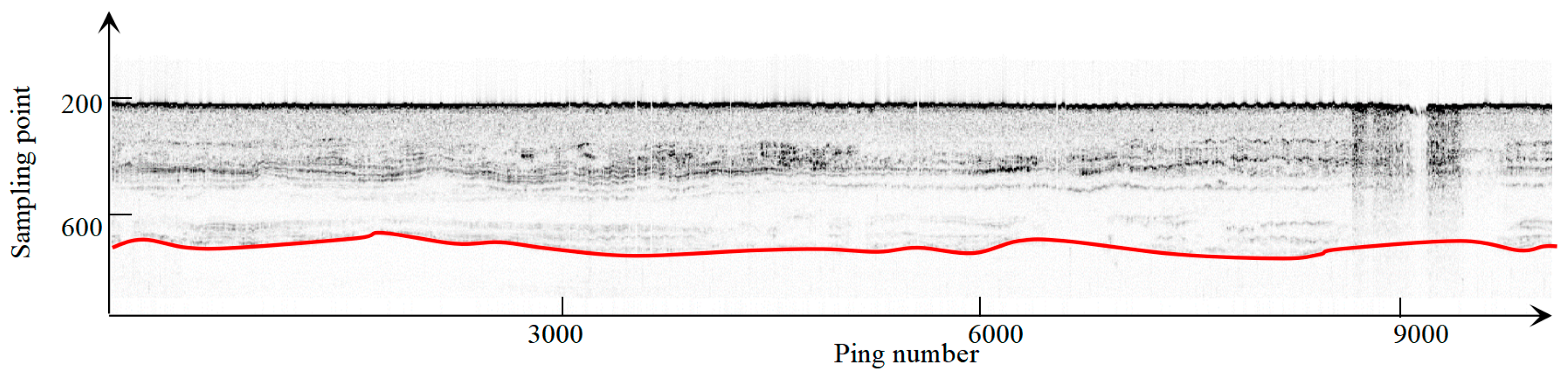
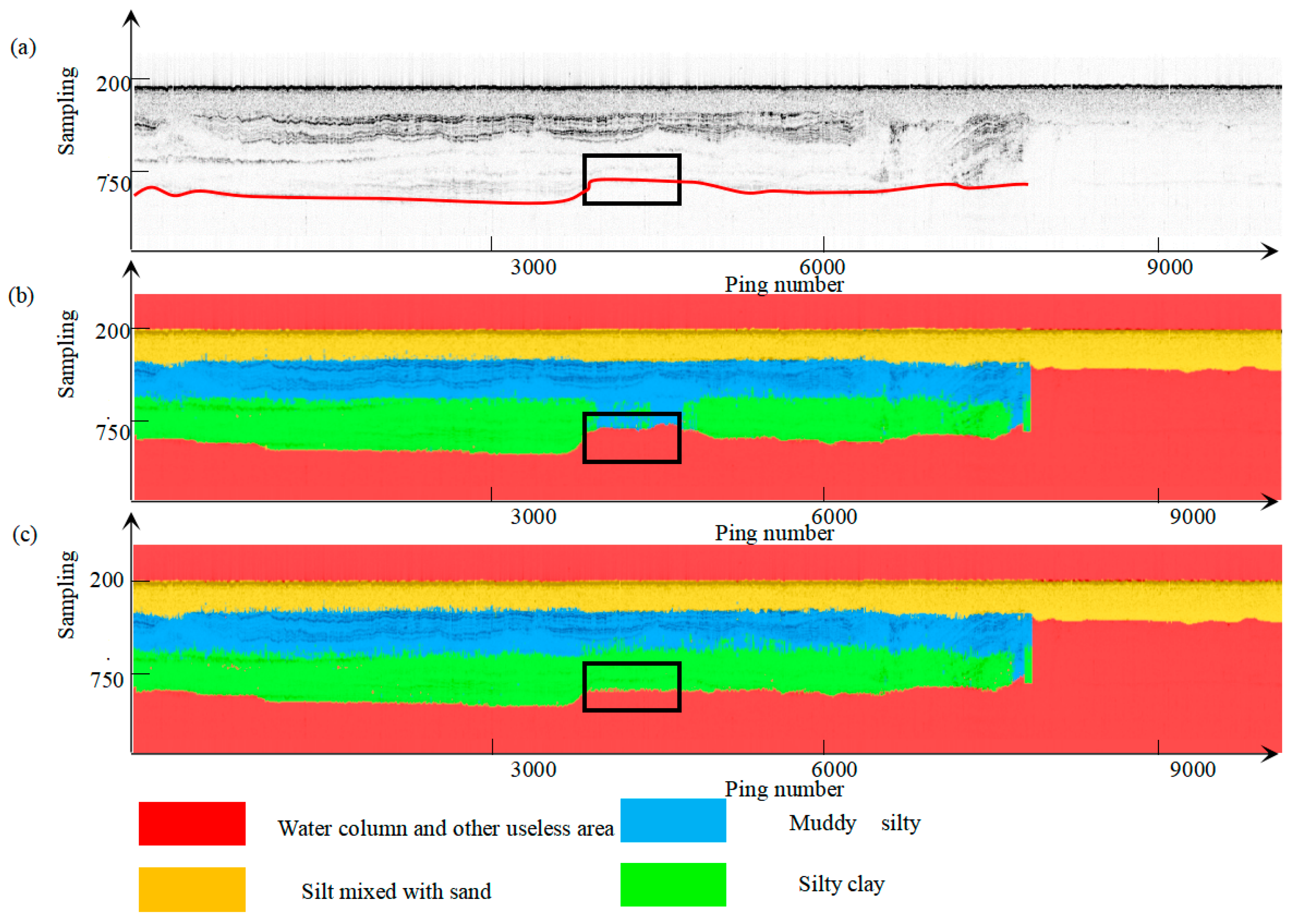
The multi-attributes can be obtained from the above. Then, post-processing is needed before putting attributes into the deep learning model. Post-processing is used to wipe out the useless information where the energy of the emitted acoustic wave is too low to convey any useful information. An SBP image is shown in Figure 3, in which, below the red line, nearly no significant reflection can be found. The acoustic wave is weak below the red line and the received signal has a low signal-to-noise ratio (SNR). Thus, the sampling points below the red line in Figure 3 should be wiped out to improve the performance of the classification method. The instantaneous attribute values of these sampling points will be set as zero.

2.3. One-Dimensional Convolution Layers and TCN Blocks

SBP emits acoustic waves through the water and underwater sediment. Then, the wave is reflected from the sediment interface, and the transducer continuously receives the reflections. The received reflections consist of a set of sampling points arranged by time. Thus, the SBP signal data form a time sequence signal. Like the seismic signal, the SBP signal can also be formulated through the convolution model, as follows: s(t) = r(t) × c(t) + n (‘∗’ means convolution). The convolution process indicates that the wave field at the current time is not affected by its values at future times but at past times. To classify a series of echo signals is to assign a label to each sampling point in the received time sequential data, thus echo signal classification is a sequence-to-sequence task.

Considering that the sequential length of a received SBP signal is large, the 1D CNN is used firstly as a high-feature extractor. Employing a 1D CNN can not only reduce the dimension of the received signals but also highlight the ability to follow models in terms of modeling contextual information.

After 1D CNN, a network that is capable of sequentially representing dynamic temporal behavior, in our case TCN, can be used to process sequential data like an SBP signal. Lots of methods have been developed for this task. TCN [41,42] is a relatively newly developed tool for the sequence-to-sequence task. Furthermore, many experiments have shown that, despite the theoretical ability of recurrent architectures to capture an infinitely long history, TCNs exhibit substantially longer memory, and are thus more suitable for domains in which a long history is required.

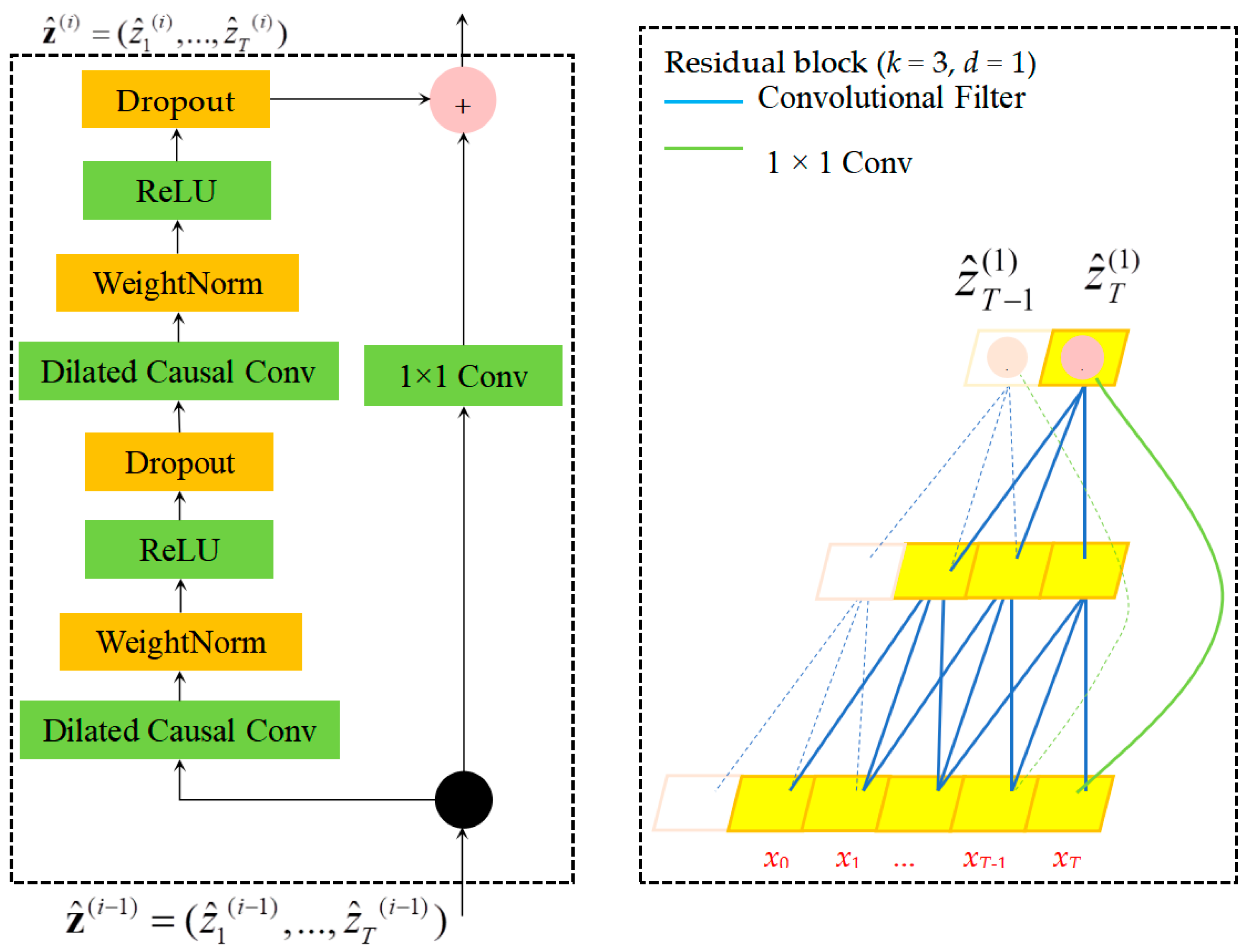
The TCN structure is shown in Figure 4. At first, a dilated causal convolution layer is put after the input. Then a normalization layer and ReLU activation, as well as a dropout layer is followed. After that, the above structure is repeated. “Causal” refers to convolutions in which an output at time t is convoluted only with elements from time t and earlier in the previous layer. The dilation layer is used to achieve a large receptive field and is thus suitable for long-length series data feature extraction. To apply the aforementioned causal convolution on sequence tasks, the idea of a residual network is introduced to better train the model, hence the concept of residual blocks. In this TCN framework, when the number of channels of the input and the output is different, a 1 × 1 convolution is used.

2.4. Cross Entropy Error Function and Class-Edge Loss Function

Loss functions form an indispensable module in the supervised learning procedure. To optimize the model parameters, a combination of cross-entropy error function and class-edge Loss function is utilized in the training process with a back-propagation algorithm.

Cross entropy error function has been widely used in classification tasks and has been proven to be effective. Since our task is a sequence-to-sequence classification task, the cross-entropy error function is also used in this paper.

We use a standard multi-class cross-entropy loss, which is denoted as:

$$L_{seg}=-{\displaystyle \sum _k{\displaystyle \sum _p{s}_k(p)\log (s_k(p)),}}$$

(7)

$\widehat{s}\in {\mathbb{R}}^{P\times K}$ denotes GT class labels in a one-hot form. p is the number of class categories. K is the number of sampling points of one ping.

3. Experiment and Results

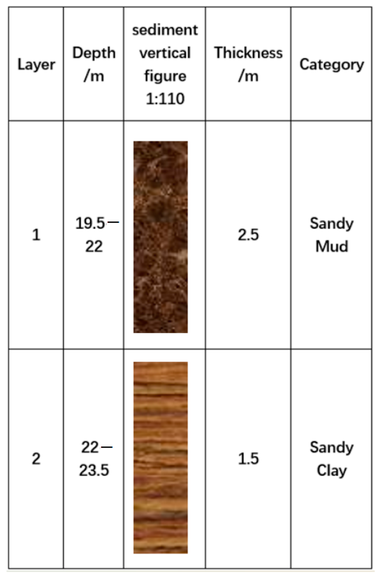
To verify the effectiveness of the proposed method, real-data experiments were performed, as described below. The study area is located in Bohai. During the SBP survey, 60 survey lines, having a total length of 240 km, were carried out using an Innomar SES 2000 Standard SBP. For this survey, a predetermined set of drill holes was planned, set to be 8 meters below the seabed’s surface. Analysis of the gathered drilling samples in the lab has led to a broad classification of the sediment in the area into two rough layers. The upper layer is primarily composed of sandy mud, while the lower is predominantly sandy clay, with minor interjections of sandy silt. Sandy mud is marked by its uneven soil quality and the abundance of coarse sand particles, along with approximately 27.3% clay content. Sandy clay consists of fine grains generally under 0.005 mm, with a few silty soil layers. The sandy silt has intermediate grain sizes, ranging from 0.005 to 0.05 mm, and the soil displays inconsistent quality, with some silt presence. Representative data from the sedimentary drilling is illustrated in Figure 5.

3.1. Criterion

To evaluate the classification performance, classic accuracy metrics, such as precision, recall, and F measure, were used to assess the chosen results. Referring to the confusion matrix, TP, TN, FP, and FN denote the numbers of true positives, true negatives, false positives, and false negatives, respectively.

Precision is defined as [43]:

$$Precise=\frac{TP}{TP+FP}$$

(8)

For class A, precision is defined as the ratio of the number of sampling points that are correctly predicted as A to the number of sampling points that are predicted as A.

The recall is defined as the ratio of the number of sampling points predicted as A to the total number of sampling points that belong to A.

$$Recall=\frac{TP}{TP+FN}$$

(9)

F-measure is the comprehension of precision and recall and is defined as follows:

$$F-measure=\frac{2Precise\cdot Recall}{Precise+Recall}$$

(10)

Intersection over union (IoU) is also used. The calculation of IoU is shown as follows [43]:

$$IoU=\frac{TP}{TP+FN+FP}$$

(11)

3.2. Experiment Setup

We evaluate our method on the data surveyed in Tianjin. The train data set contains 14,900 training time series, while the test data set contains 1000 test time series. There are 24,000 training pings from 6 sediment categories. The sediment categories selected from the surveyed area are silt mixed with sand, muddy silty clay, and silty clay. Each category has a 5000 training time series. Our work is based on the sequence data rather than the profile image, as the image can only reflect the structures of the sediment distribution, while the physical properties cannot be inferred from the profile. Thus, every single ping is used as a test or train data. A set consisting of ping data of different survey lines was collected, with other survey line data being divided among the training, validation and test sets, with all of the data then used for the model building. Many thousand aspects of train or test data can be obtained. Our model is trained using the training set and is tested on the validation set. The length of each time series is 1250.

The training samplings were selected from the pings of the surveying line closest to the holes, or some surveying lines which are noise-free and in which the sediment types can be easily determined. According to the holes, the sediment types and the sediment compositions can be obtained [44,45]. The training set is built as far as possible to include different sediment types and distributions.

(1) Parameter Settings and Network Training: The Adam solver was adopted as the gradient descent optimization method. The learning rate γ was initialized to 0.0005. The proposed network was trained for 20 epochs with a batch size of 15, and, after 5 epochs, the learning rate was reduced by being multiplied by a descending factor equaling 0.01. Our proposed method was implemented on the deep learning framework Matlab. All experiments were performed on a computer with an Intel Core i7-10750H CPU, 16 GB RAM, and NVIDIA RTX 2060 GPU.

3.3. Method Validation

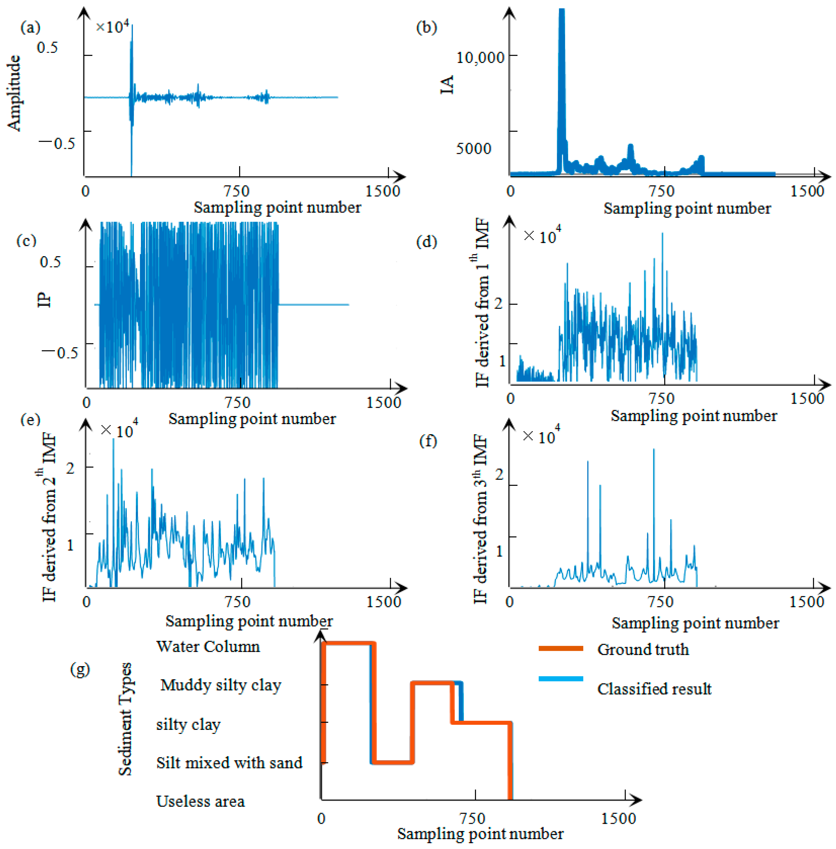
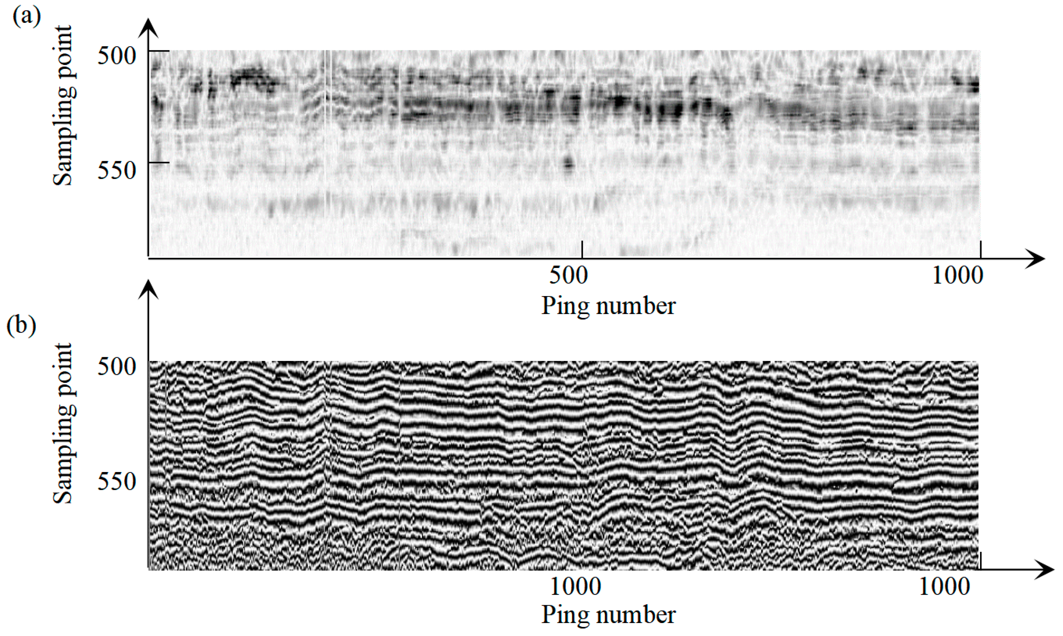
First, we obtained the instantaneous attributes. The IF, IA and IP data of the 1000th ping are shown below in Figure 6. The sampling points with high IA value means that the impedance contrast here is very strong and the sediment density and velocity have large changes. Figure 6b,c show the IP and IA data of the 1000th ping, respectively. The IP image and IA image (namely the SBP image, as the SBP image is always built based on IA data) are built by converting the IP and IA data values into 0~255. The comparison between the IA image and the IP image is shown in Figure 7. From the IP image, it can be confirmed that the details of reflections have been highlighted, and that continuous horizons and some tiny structures can be imaged. IF data is related to the lithology of the sediment, as has been proven by many researchers, though physical information cannot be discovered from the IF image directly. Intuitively speaking, IF derived from the first IMF has a high time scale and can be influenced easily, and IF derived from the third IMF has a low time scale and is robust against noise. IF series of different IMFs are shown in Figure 6d–f.

Figure 6g shows the 1000th ping data series of this survey line. The predicted result and the GT are also shown. It can be noted that the sediment types have been classified well, a continuous sediment boundary was also obtained, and the sediment distribution is consistent with the ground truth.

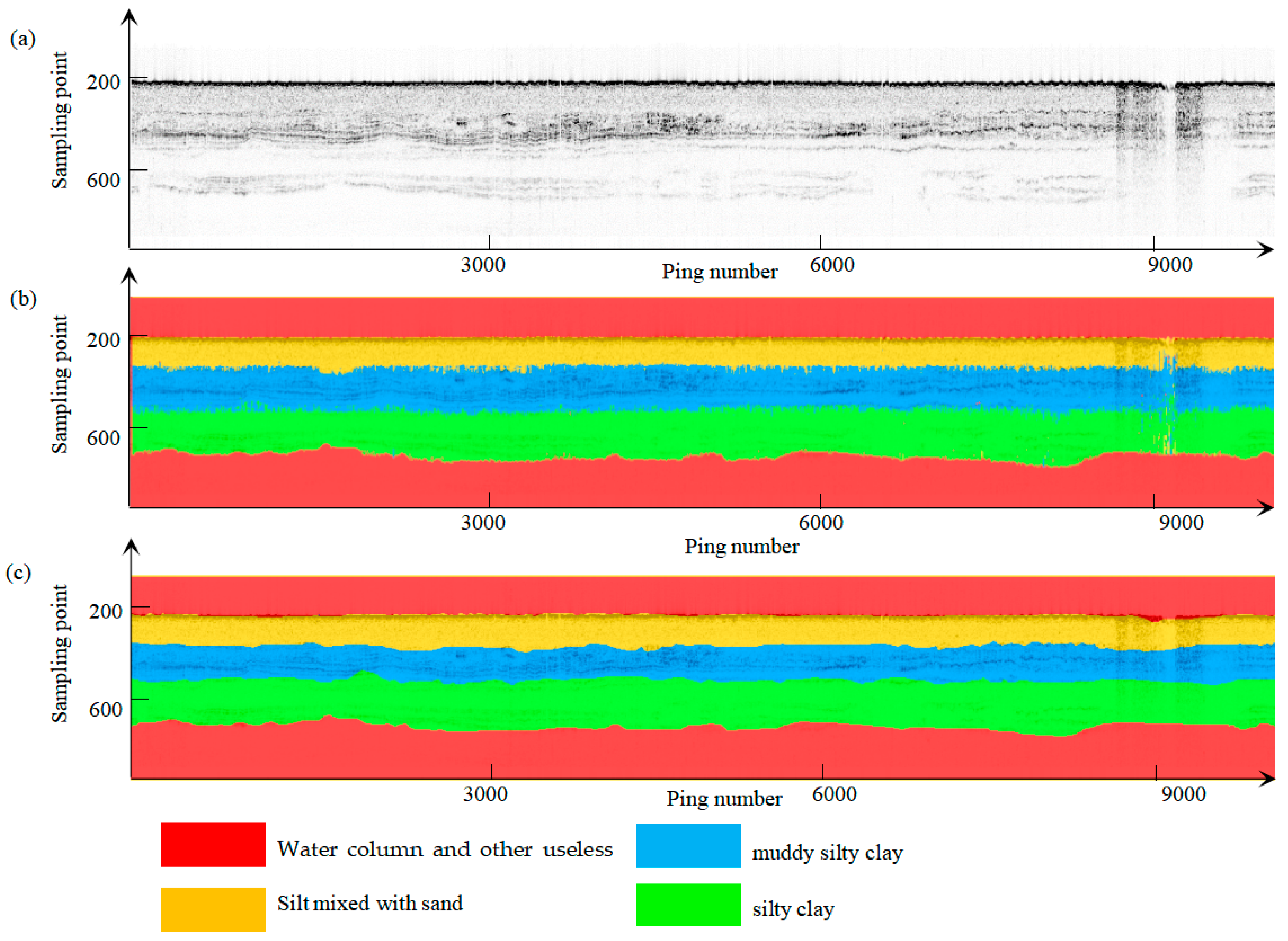
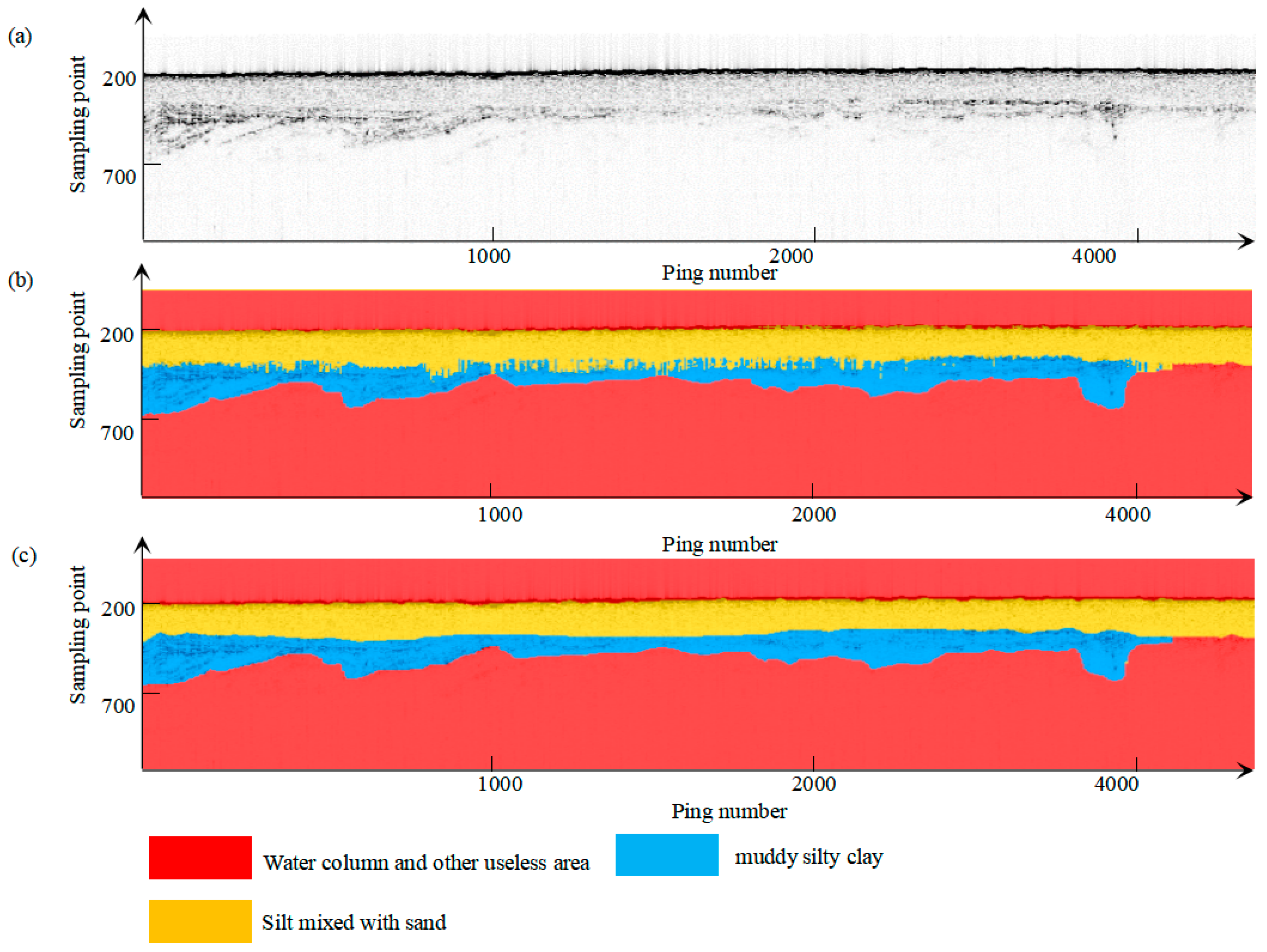
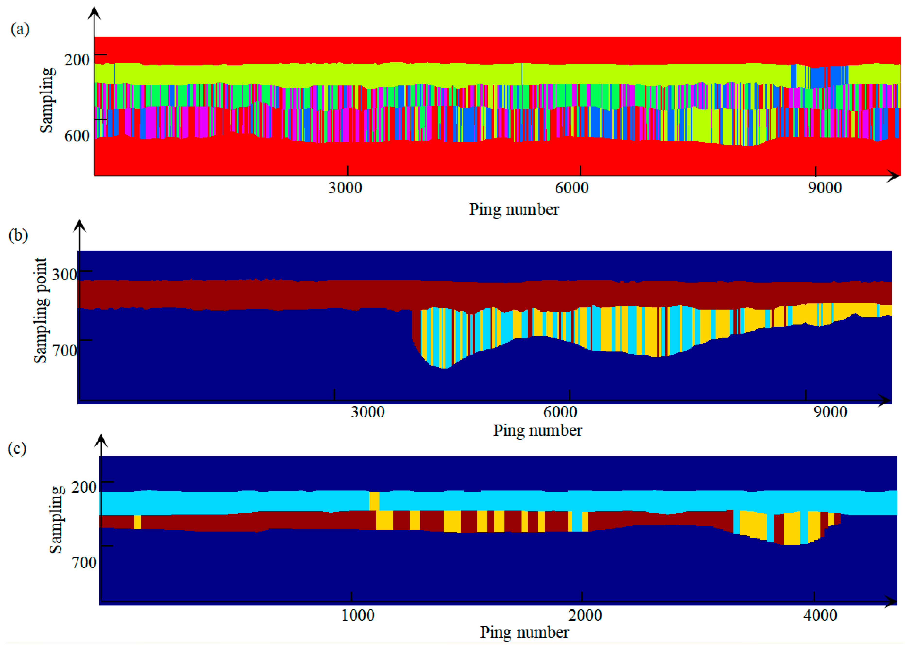
Using the proposed method to classify the whole surveying line, the classified results of all pings are shown in Figure 8, in which different sediment types are signed with different colors. The red area shows the water column area and other useless areas, the yellow area shows the silt mixed with sand, the blue area shows the muddy silty clay, and the green area shows the silty clay area. Different sediment types of this profile are superimposed on the SBP image. Additionally, the ground truth is superimposed with the SBP image in Figure 8. From the result, it can be concluded that the great lateral continuity of sediment interfaces has been kept and that the classified sediments are highly consistent with the ground truth.

A phenomenon that should be noted is that the same sediment layer contains more than one horizon. Different sediment types may have similar horizon distributions. For example, the horizon distribution of silt mixed with sand is similar to the horizon distribution of muddy silty clay. As shown in Figure 8a, there are many parallel horizons inside both these two sediments. These two sediments can hardly be separated from the characteristics of only horizon distribution. In this complex situation, we think that the combination of multiple attributes has played an important role in the accurate sediment classifications.

Moreover, the classified results have been evaluated by the criterion described. The evaluated results show that the proposed method achieved a value of 80%. The result is listed in

Table 1. Analysis of the classification performance in Figure 8.

Class Number	Precision	Recall	F-Measure
Water column and other useless areas	0.86	0.85	0.85
Silt mixed with sand	0.95	0.88	0.91
muddy silty clay	0.98	0.92	0.95
silty clay	0.82	0.97	0.99

.

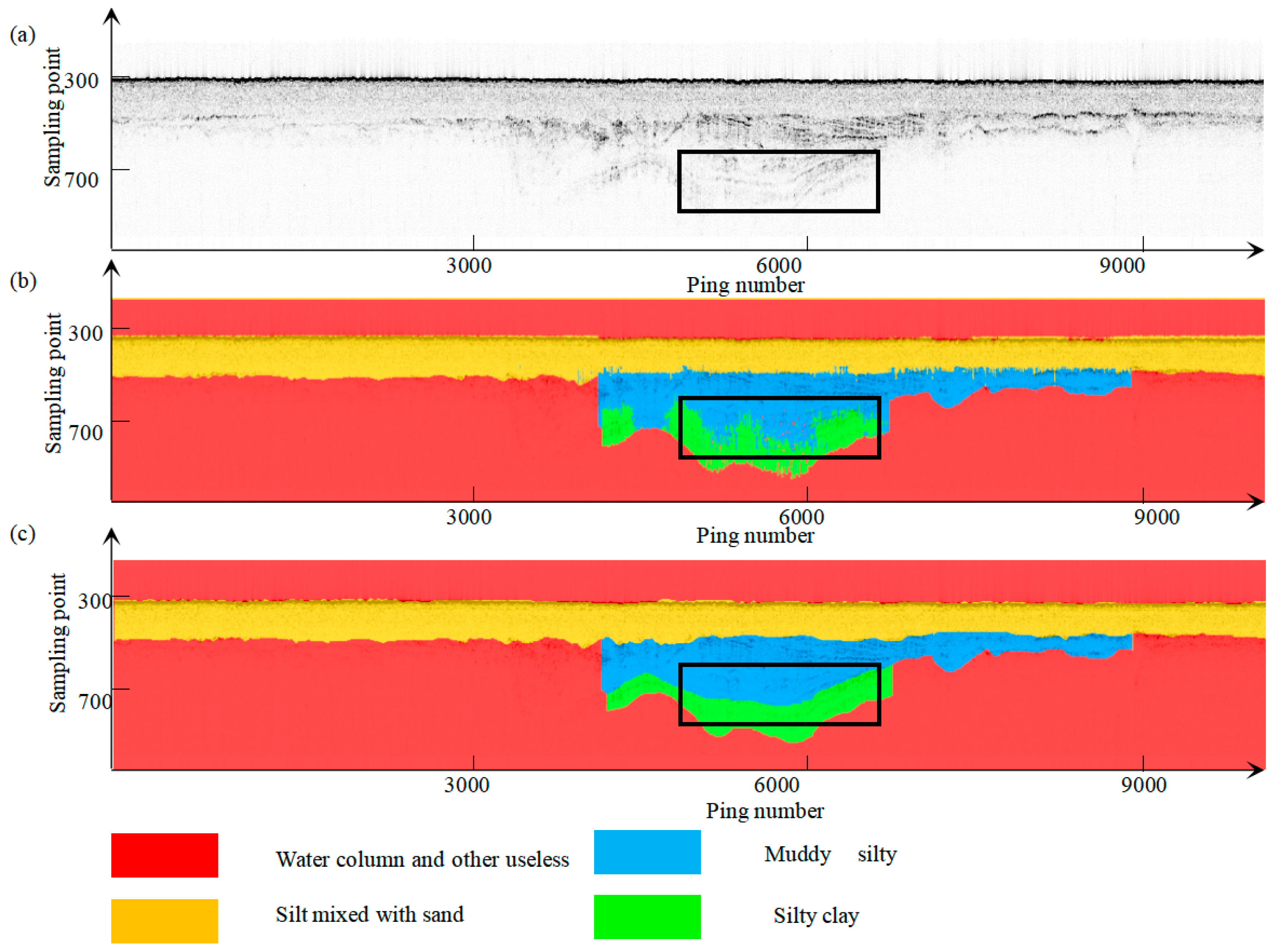
The test class results for the other test line are shown in Figure 9 and the quantitative indexes are shown in

Table 2. Analysis of the classification performance in Figure 9.

Class Number	Precision	Recall	F-Measure
Water column and other useless areas	0.98	0.99	0.98
Silt mixed with sand	0.87	0.88	0.87
muddy silty clay	0.92	0.80	0.86

. This survey line has two types of sediments. The thickness of the first layer is relatively the same; SBP did not penetrate the second layer completely, and the second layer showed varying thickness on the SBP image. The vertical distribution of the two layers is outlined by manual interpretation. The method in this paper achieves the classification of two layers of sediment well, but there are some deviations in the prediction results at the boundary between the first layer and the second layer, which is caused by the small difference in acoustic impedance between the two layers of sediment in some areas.

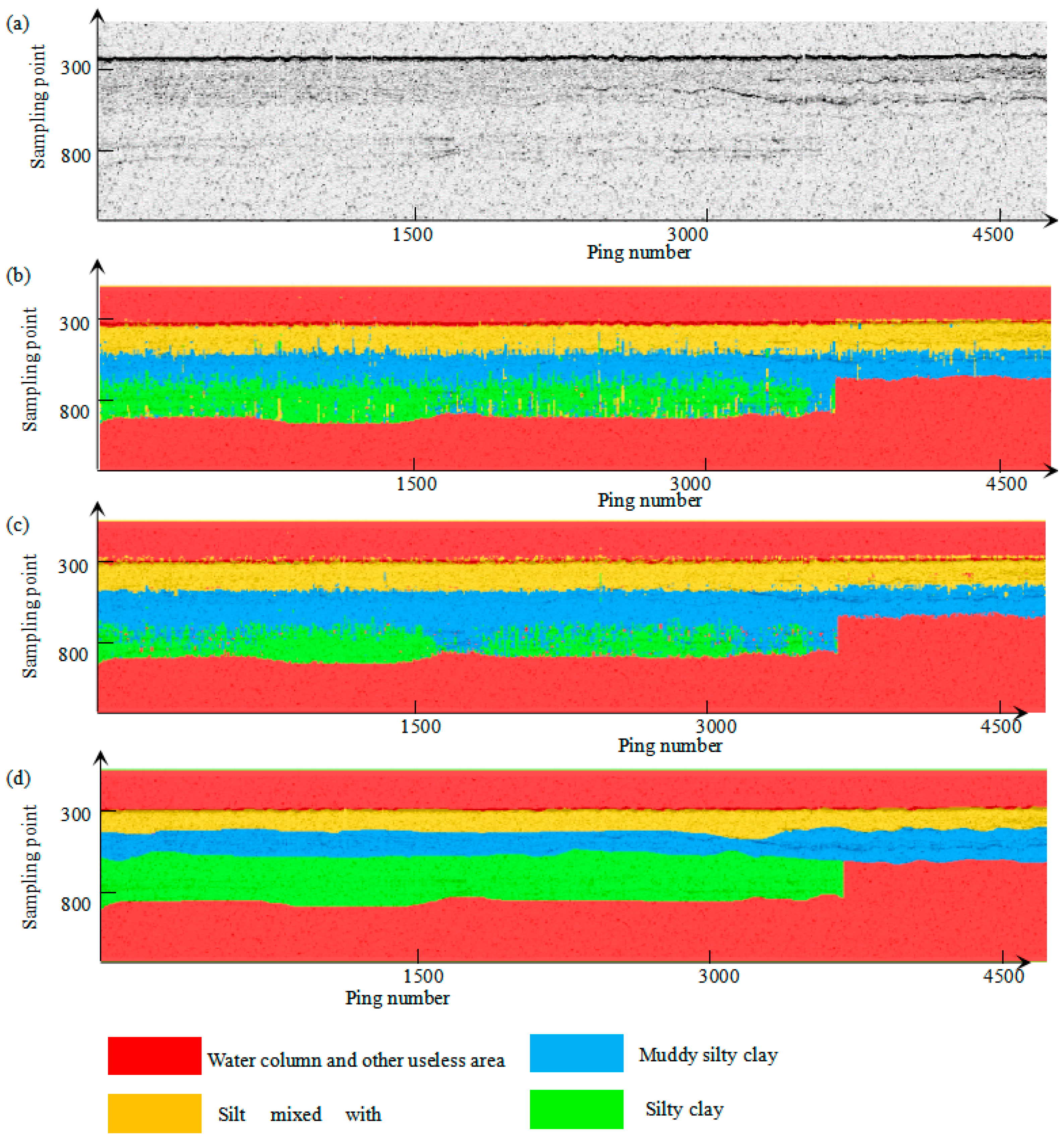
The data of the third survey line contain three types of sediment. The silty clay is only present in the middle of the survey line. The overall classification effect of the data is good, but the classification effect is poor at the boundary between the second type of sediment and the third sediment, as shown in Figure 10. And the quantitative indexes are shown in

Table 3. Analysis of the classification performance in Figure 10.

Class Number	Precision	Recall	F-Measure
Water column and other useless areas	0.98	0.99	0.99
Silt mixed with sand	0.92	0.91	0.91
muddy silty clay	0.73	0.75	0.74
silty clay	0.82	0.88	0.85

. We think this is because the echo intensity and signal-to-noise ratio of the SBP signal decreases with the increase of depth, so that the classification effect of the lower substratum is worse.

We calculated and listed the IoU of the three survey line data, as shown in

Table 4. IoU of the classification performance.

Experiments	IoU
Experimental result in Figure 8	0.80
Experimental result in Figure 9	0.94
Experimental result in Figure 10	0.91

. Because the algorithm has a good classification of non-layer areas, such as the water area, which account for a large proportion of the data, the overall IoU accuracy is relatively good. The time cost is shown in

Table 5. The time cost of the classification performance.

Experiments	Time
Experimental result in Figure 8	81.78 s
Experimental result in Figure 9	43.77 s
Experimental result in Figure 10	71.78 s

.

4. Discussion

4.1. Effectiveness of Multi-Attributes

In this section, the performance of the proposed MATCN algorithm was compared with the method using only original data. Replacing the multi-attribute input in the MATCN with the single original data input, we can test the effectiveness of the multi-attribute input. The sediment distribution does not seem continuous enough. There are many predicted outliers in the second layer. It can be seen from Figure 11 that the other methods acquired classification results that appear to include more outliers than the proposed method. It can be concluded that the competing model based on a single input performed poorly when compared with the proposed method.

The MATCN model adopts a multi-attributes scheme and generally works better than a model that uses a single input, as shown in Figure 11b,c.

Our MATCN achieves good numerical performance. We attribute this to the combination of TCN-based and attribute-based classifications.

4.2. Determination of Red Line

After calculating the multi-attributes, processing is needed before they are input into the deep learning model. Sampling points located below the manually determined red line are recognized as useless, and the instantaneous attribute values of these sampling points will be set as zero. As it is determined manually, bias can be induced when drawing the red line. Usually, the red line is the lowest boundary of the reflector, and the induced bias can make the red line higher or lower than the lowest boundary of the reflector. To analyze the influences of line bias on the final predicted results, two experiments have been employed. In the first experiment, the determined red line is slightly higher than the low boundary of the reflector. Figure 12b shows the predicted result when using this red line to wipe out useless sampling points. The black rectangle in Figure 12 indicates that the prediction accuracy is not good enough. In the second experiment, the determined red line is lower than the lowest boundary of the reflector. Figure 12b shows the predicted result when using this red line to wipe out useless sampling points. The black rectangle indicates that the proposal has achieved good performance. The analysis above shows that it would be better to draw the red line a little lower than the low boundary of the reflectors.

4.3. Comparisons

In this section, the performance of the proposed method is compared with a classification-based method [46]. This classification method chooses the horizons first. Then, based on the constraint of the horizons, various features are extracted from the layers, and the sediment types are classified based on various features. The result of the classification is shown in Figure 13, and, with the exception of the first layer, it is found that there are a large number of misclassifications. This is because deep layer echoes are weak, and it is difficult to extract effective features. Compared with the method in this paper, the effect is not good. In addition, only unsupervised classification can be achieved, and it is difficult to determine the sediment types.

4.4. Limitations and Future Works

It is hard to obtain an accurate sediment boundary as the lateral characteristics have not been taken into consideration. When the sediment distribution or the reflector distribution is complex, the performance of the proposed method is worse than in other situations. Figure 11 shows that the proposed method is robust to noise to some degree; however, it should be noted that the performances of the proposed method in noise-free situations are far better than in noisy situations. In addition, overfitting should also be noted. Considering these limitations, we think a transformer model can be introduced into this sediment classification task. More efforts in the field of marine sediment classification should be made to simultaneously consider the latent characteristics of SBP data and the characteristics of SBP data along pings. Another important future work is the establishment of a train sampling set, different SBP data in different areas as well as corresponding core-holes should be employed to build the train data set.

5. Conclusions

In this paper, we present an MATCN for sediment classification in SBP data, considering the IA, IF, and IP data classification potentials, which fuse multi-attributes to explore the latent sediment characteristics. The sediment classification task based on sub-bottom acoustic signal is molded as a time-sequence-to-sequence task and a novel deep learning model was constructed by combining 1D CNN with TCN to achieve better feature extraction performance. Then, multi-attributes were put into the deep learning model to predict the sediment types. Our experiments show that MATCN is an effective architecture that produces sub-bottom sediment maps.

In future works, we will combine more prior characteristics in MATCNs with the data-driven learning framework, such as the latent distribution of the horizons. The transformer model can also be introduced into this sediment classification task. In addition, we also plan to apply the deep learning-based method to the data of other water areas and to attempt to develop this form of method to the direct prediction of particle sizes.