
Visualized Experimental Study of Soil Temperature Distribution around Submarine Buried Offshore Pipeline Based on Transparent Soil


Abstract
1. Introduction
2. Test Method and Process
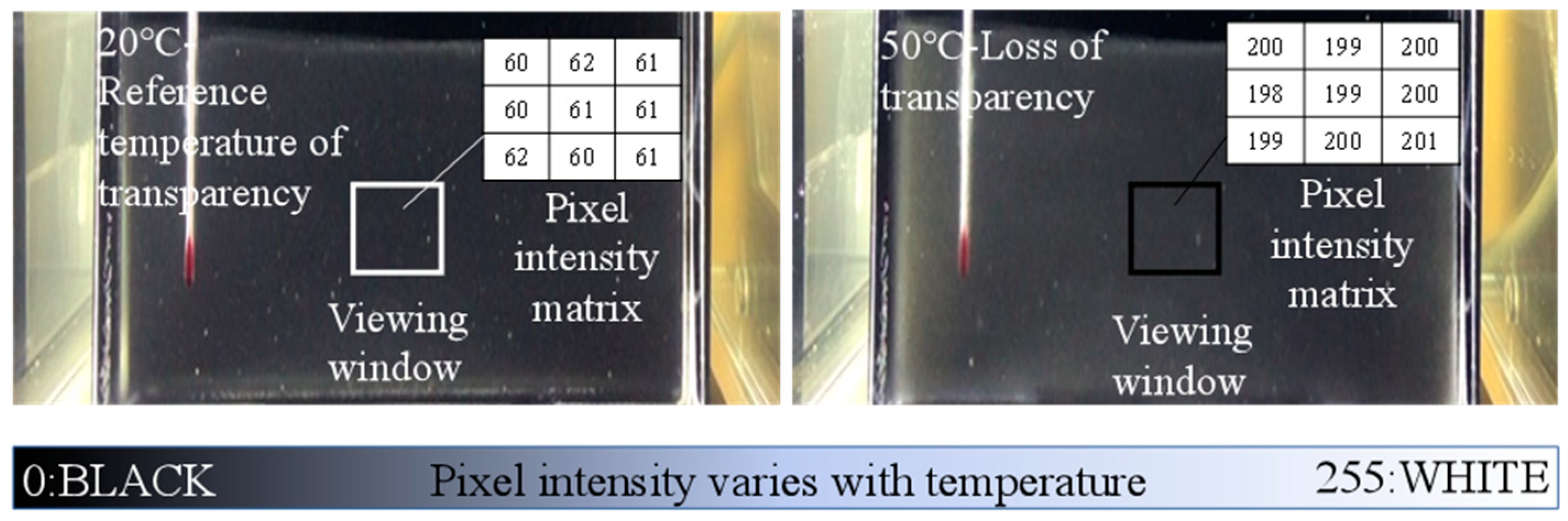
2.1. Test Method for Transparent Soil
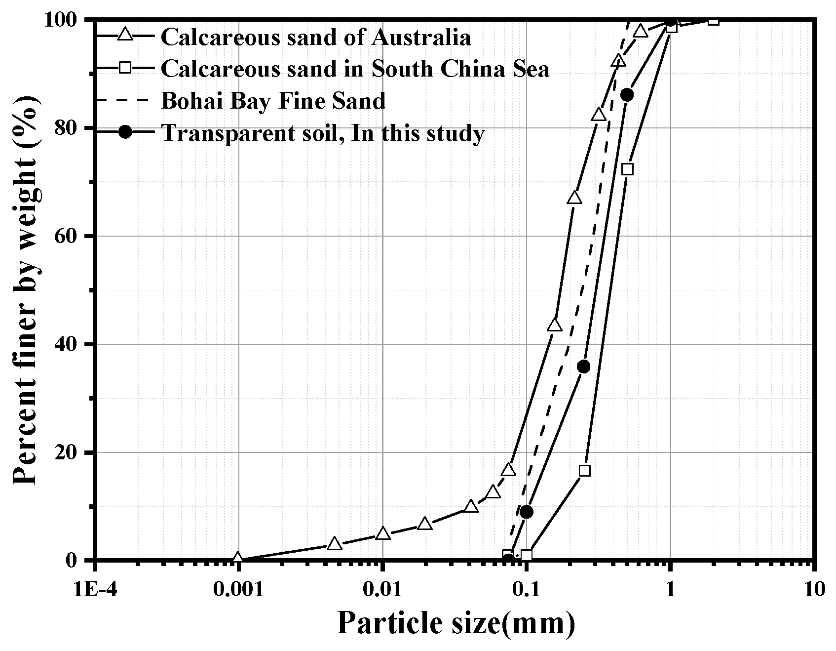
2.2. Test Materials
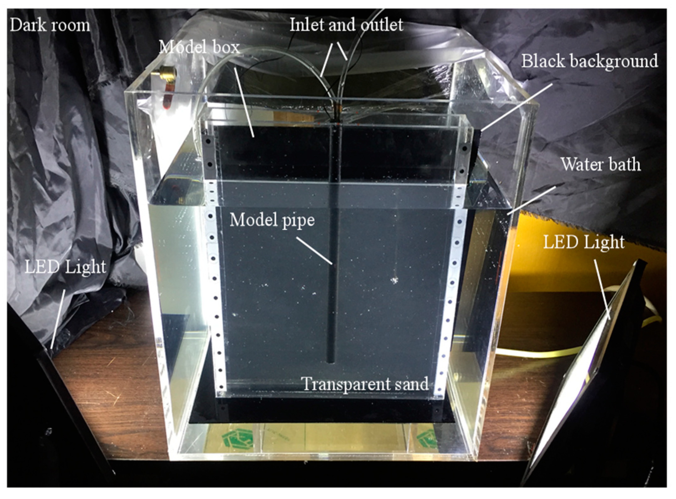
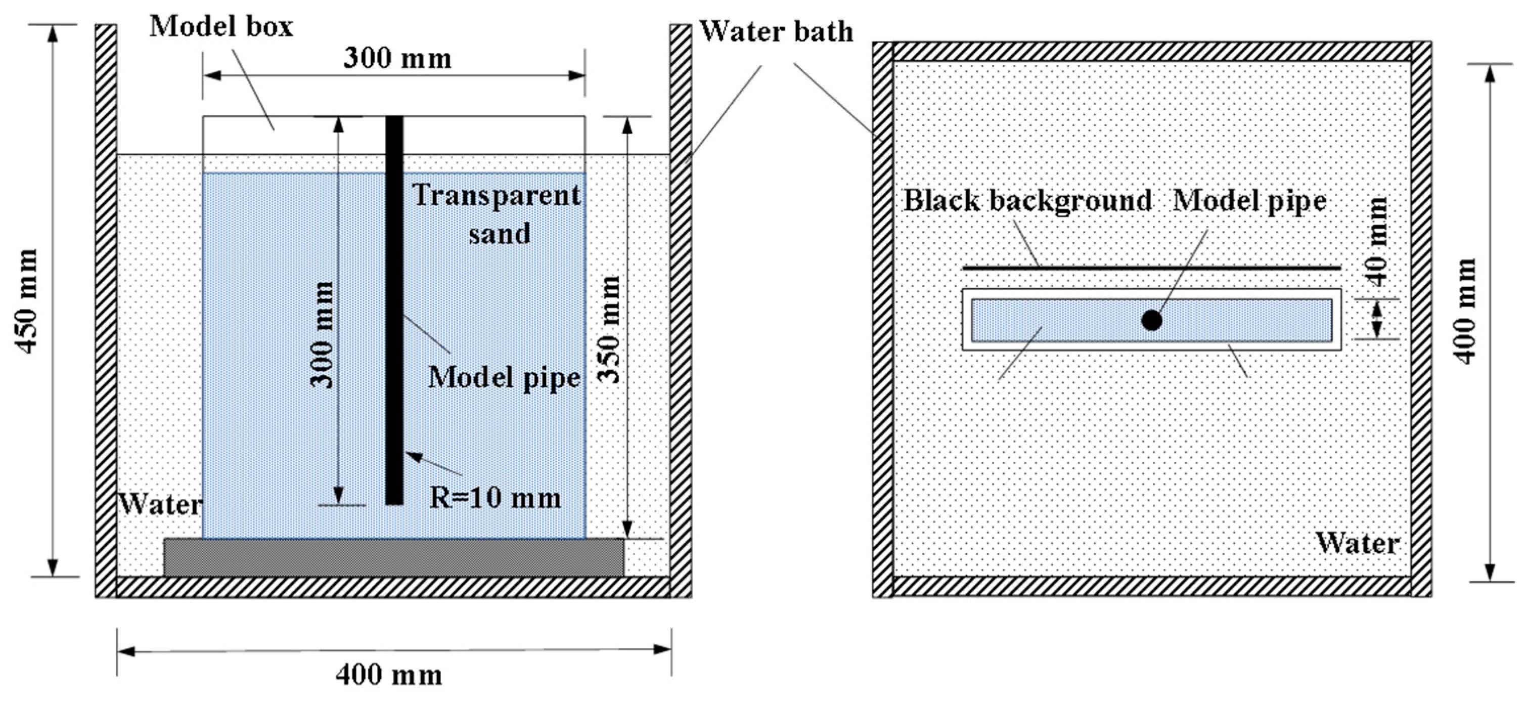
2.3. Test Apparatus for Transparent Soil
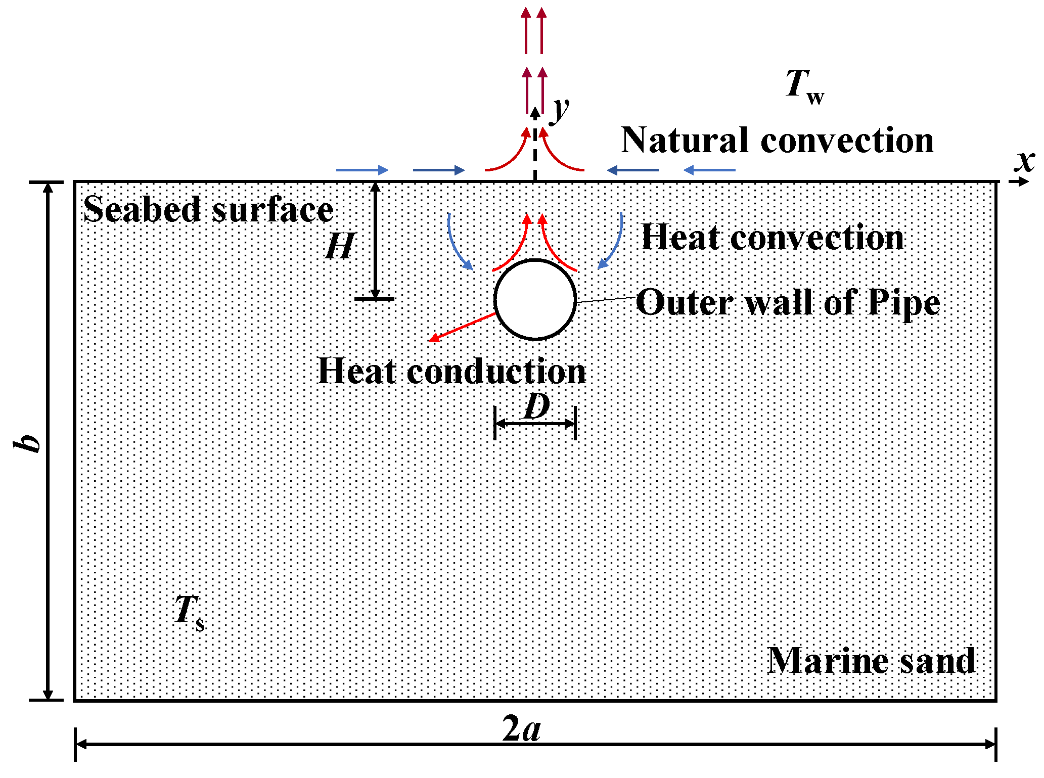
2.4. Numerical Simulation Method
- (1)
- Mathematical model
- (2)
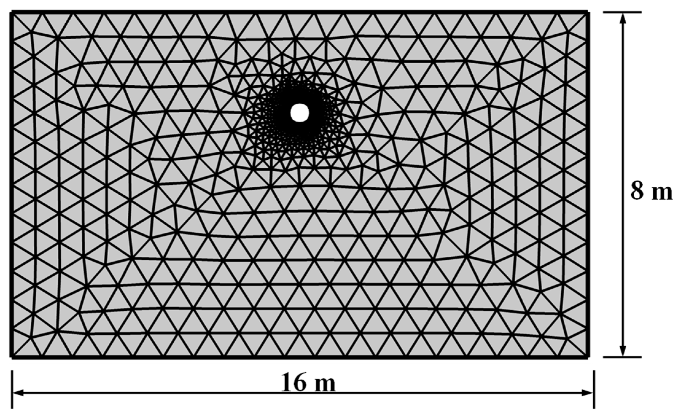
- Numerical solution
2.5. Test Procedures and Progresses
3. Experimental Results and Discussion
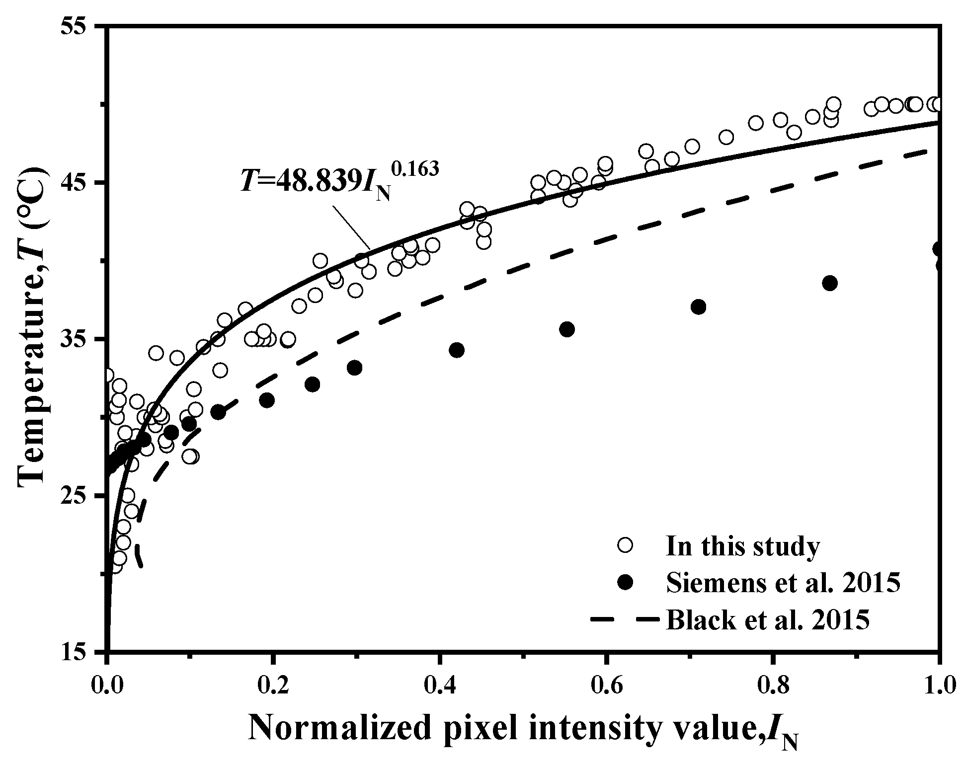
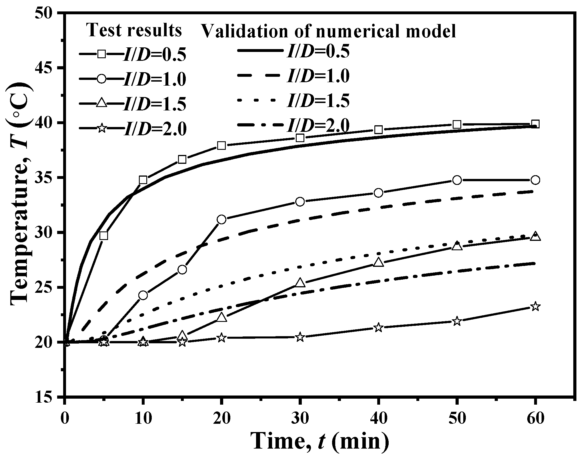
3.1. Calibration Test
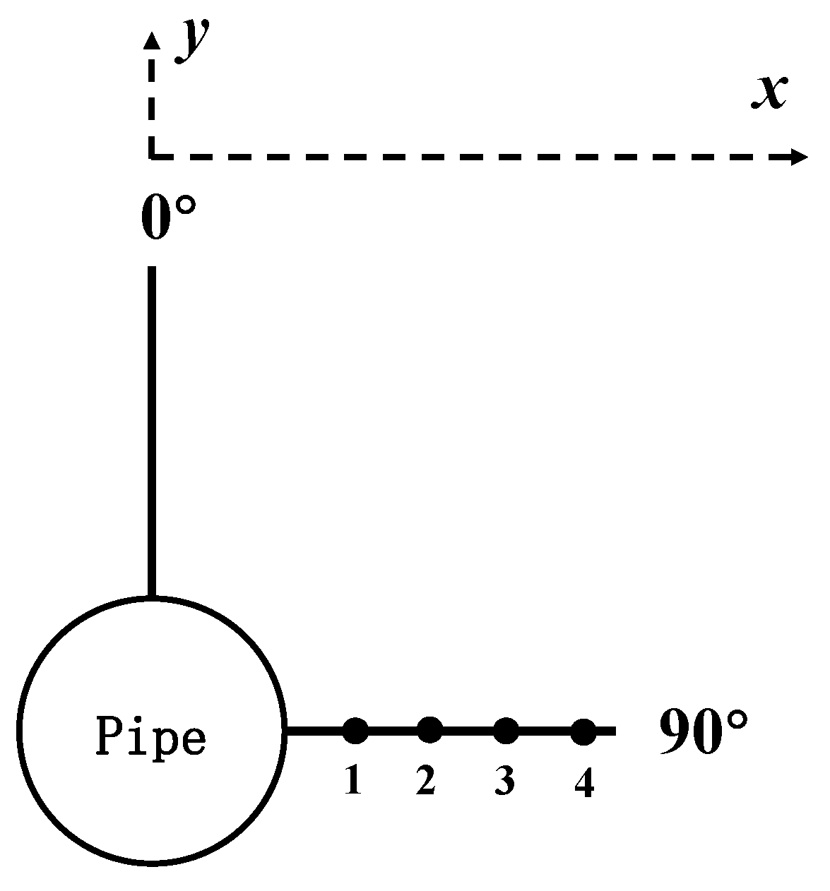
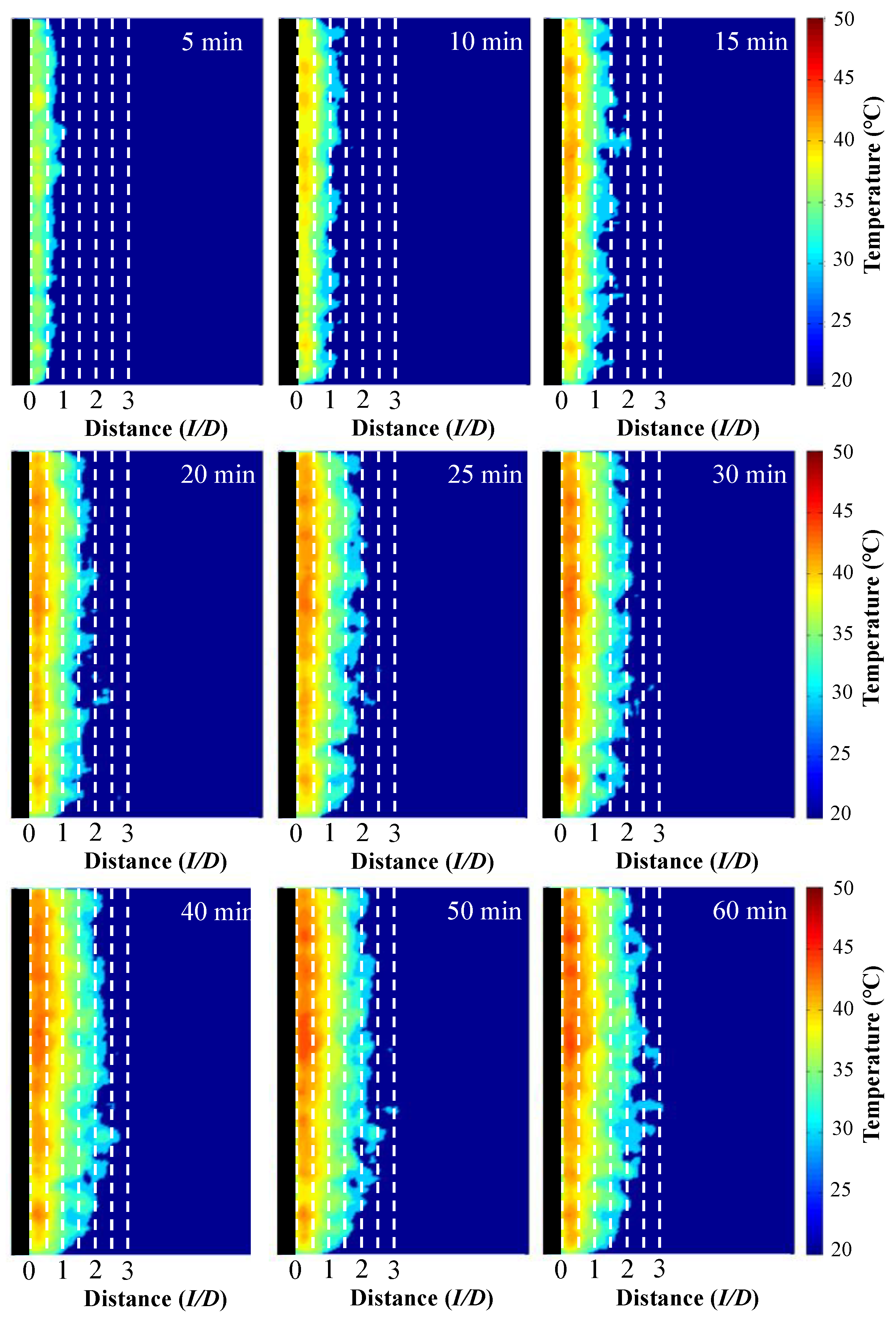
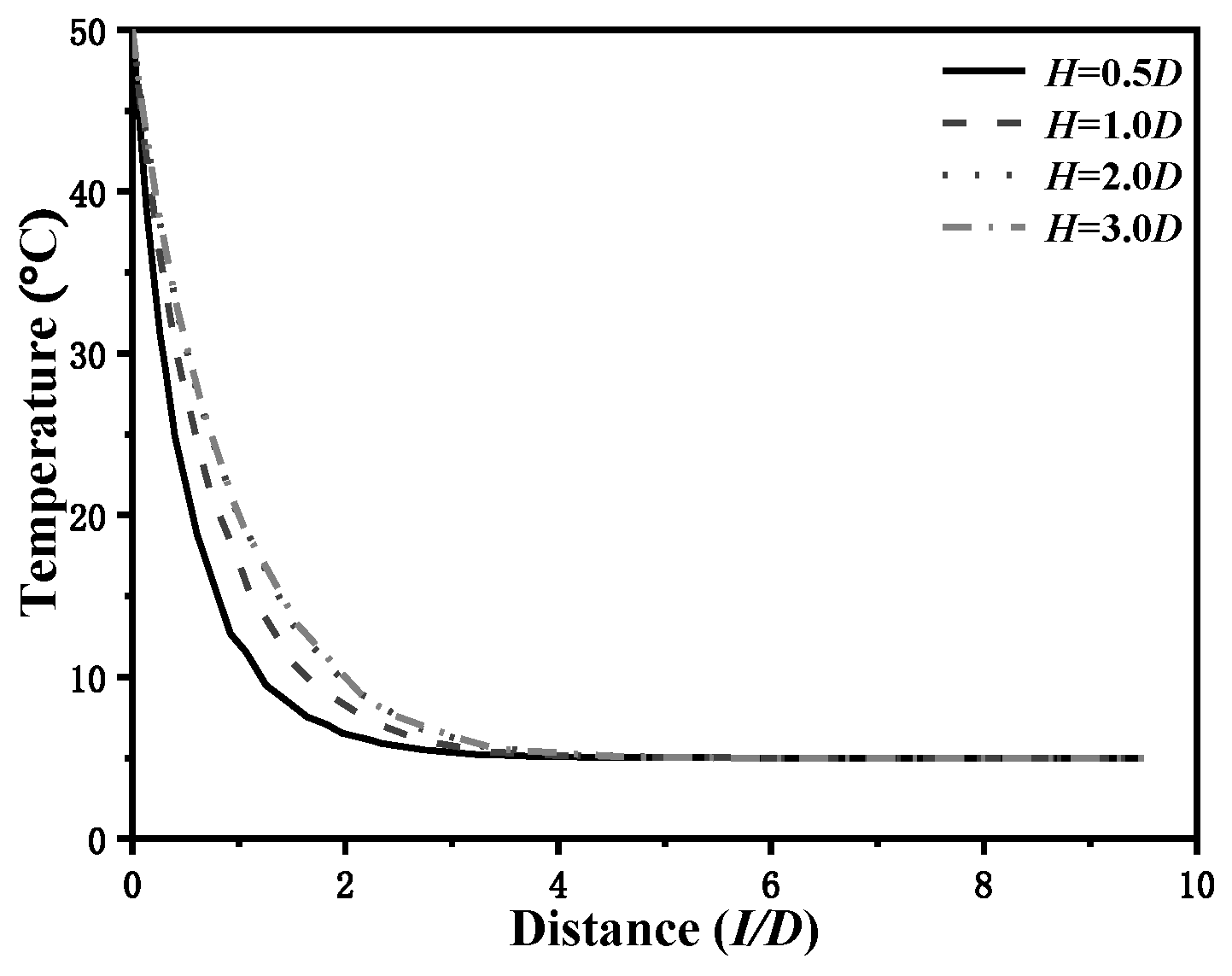
3.2. Horizontal Temperature Distribution of Soil around Pipeline
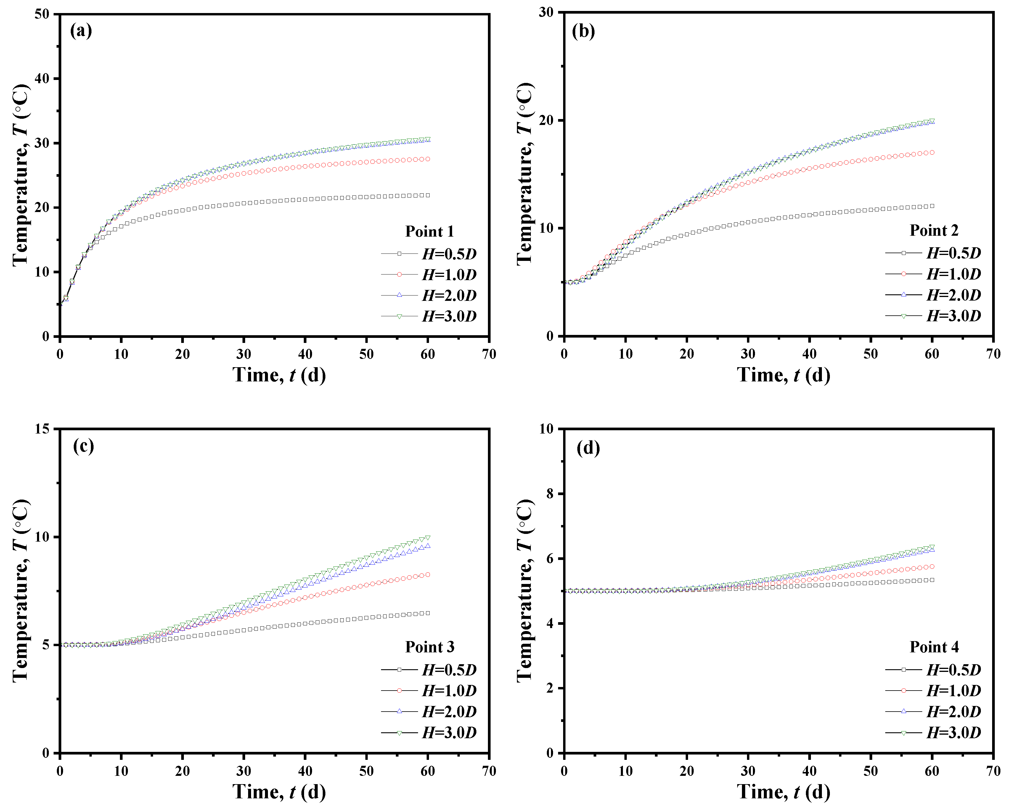
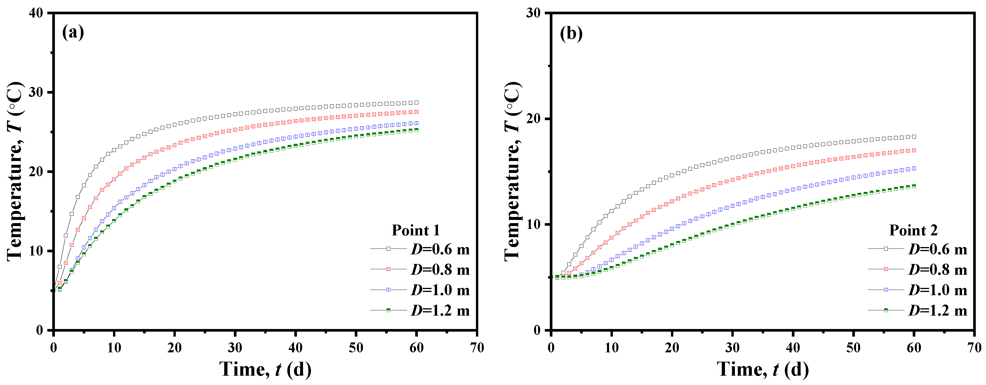
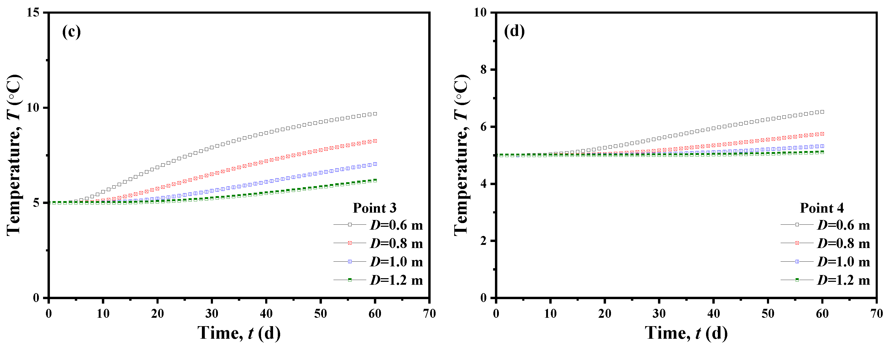
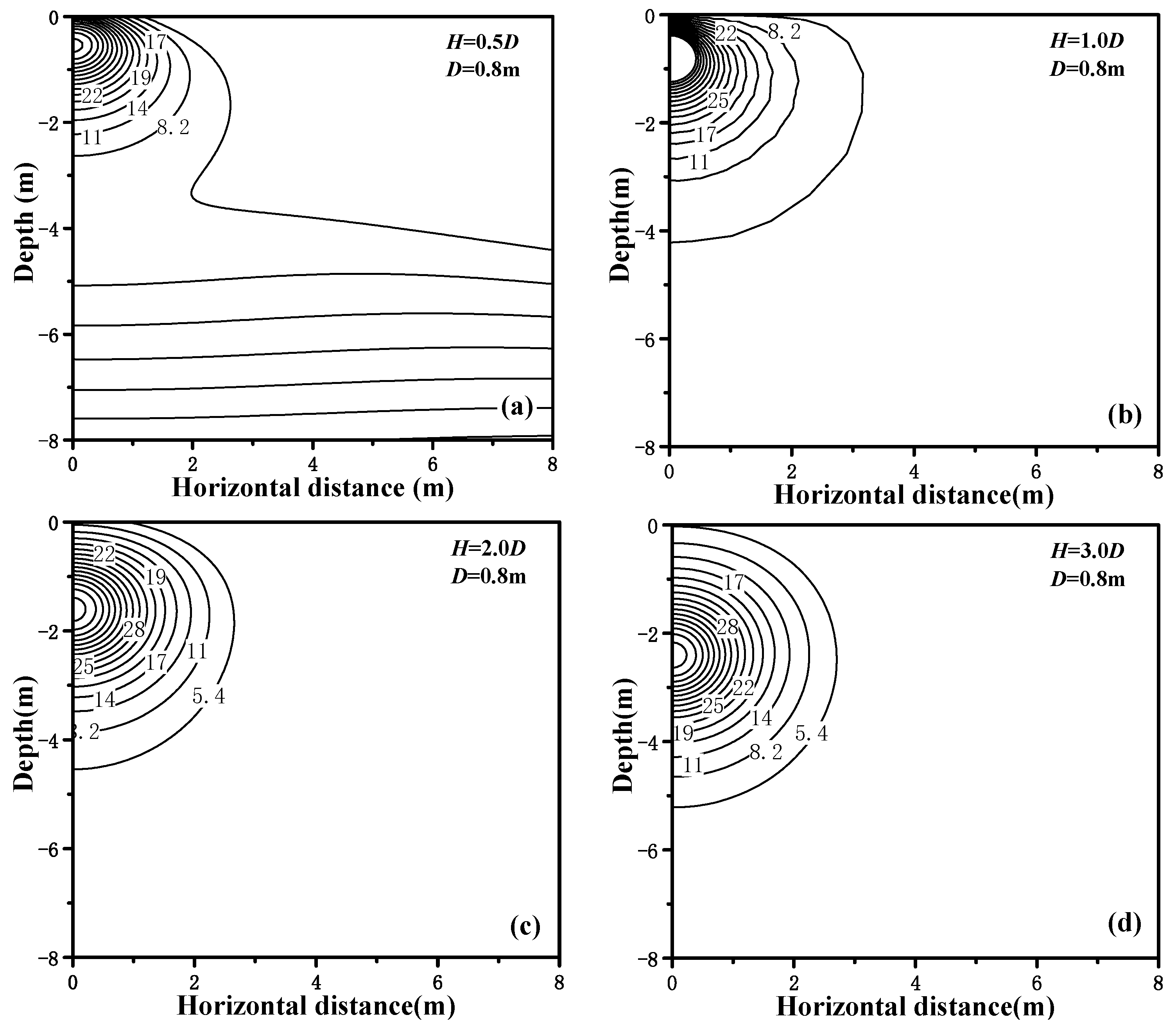
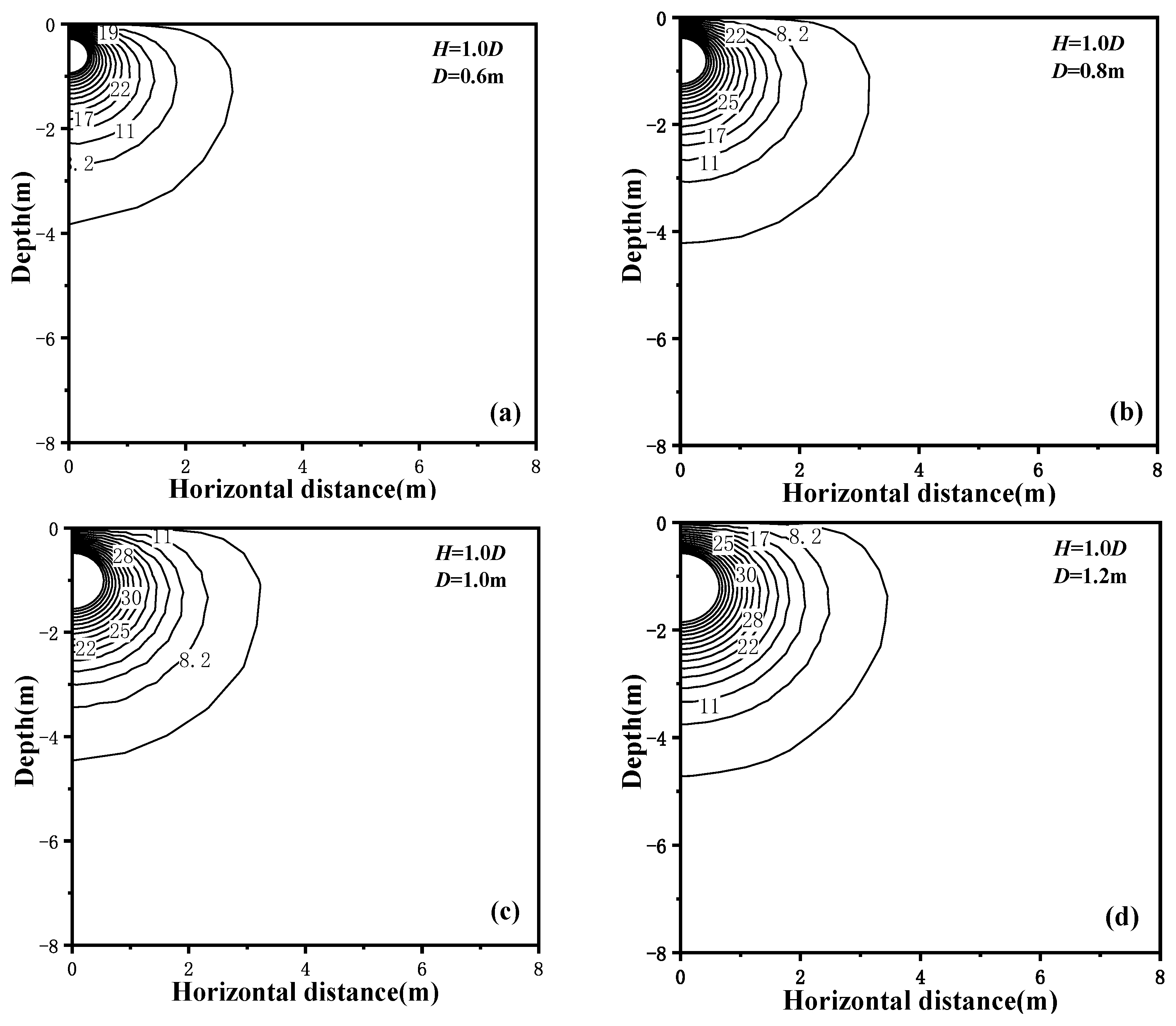
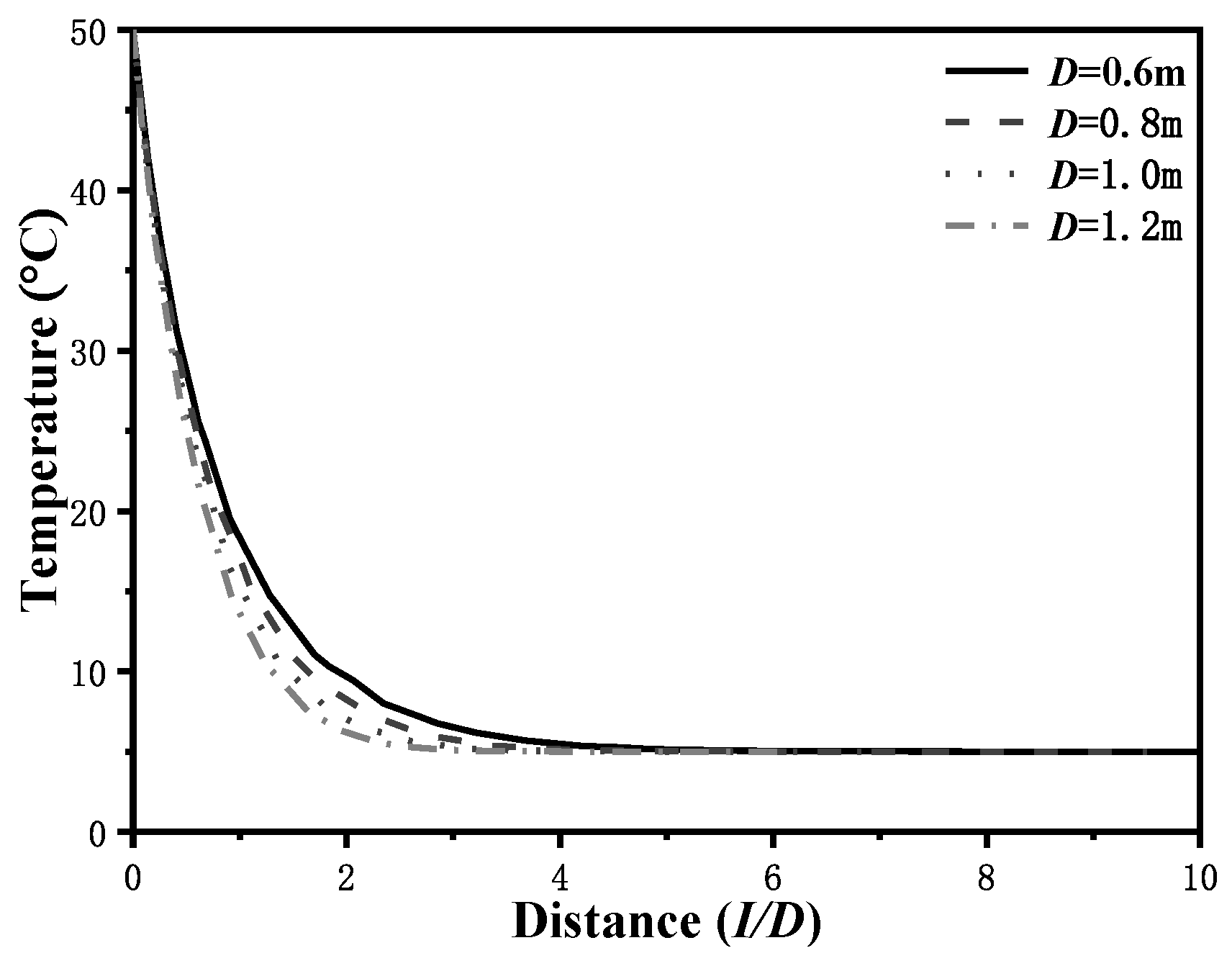
3.3. Influence of Buried Depth and Pipe Diameter on Temperature Field
4. Conclusions
Author Contributions
Funding
Institutional Review Board Statement
Informed Consent Statement
Data Availability Statement
Acknowledgments
Conflicts of Interest
References
- Yang, X.; Shi, X.; Zhao, J.; Yu, C.; Gao, H.; Chen, A.; Lu, Y.-Z.; Chen, X.; Lin, W.; Zeng, X.; et al. Bottom Water Temperature Measurements in the South China Sea, Eastern Indian Ocean and Western Pacific Ocean. J. Trop. Oceanogr. 2018, 37, 86–97. [Google Scholar] [CrossRef]
- Yu, J.; An, C.; Tang, Q.; Zhang, J.; Zhang, Y. Heat Transfer Characteristics of Subsea Long-Distance Pipeline Subject to Direct Electrical Heating. Geoenergy Sci. Eng. 2024, 234, 212679. [Google Scholar] [CrossRef]
- Yuan, Q.; Luo, Y.; Shi, T.; Gao, Y.; Wei, J.; Yu, B.; Chen, Y. Investigation into the Heat Transfer Models for the Hot Crude Oil Transportation in a Long-Buried Pipeline. Energy Sci. Eng. 2023, 11, 2169–2184. [Google Scholar] [CrossRef]
- Barletta, A.; Zanchini, E.; Lazzari, S.; Terenzi, A. Numerical Study of Heat Transfer from an Offshore Buried Pipeline under Steady-Periodic Thermal Boundary Conditions. Appl. Therm. Eng. 2008, 28, 1168–1176. [Google Scholar] [CrossRef][Green Version]
- Lu, T.; Wang, K. Numerical Analysis of the Heat Transfer Associated with Freezing/Solidifying Phase Changes for a Pipeline Filled with Crude Oil in Soil Saturated with Water during Pipeline Shutdown in Winter. J. Pet. Sci. Eng. 2008, 62, 52–58. [Google Scholar] [CrossRef]
- Rossi di Schio, E.; Lazzari, S.; Abbati, A. Natural Convection Effects in the Heat Transfer from a Buried Pipeline. Appl. Therm. Eng. 2016, 102, 227–233. [Google Scholar] [CrossRef]
- Li, Y.; Zhou, H.; Liu, H.; Ding, X.; Zhang, W. Geotechnical Properties of 3D-Printed Transparent Granular Soil. Acta Geotech. 2021, 16, 1789–1800. [Google Scholar] [CrossRef]
- Iskander, M.; Lai, J.; Oswald, C.; Mannheimer, R. Development of a Transparent Material to Model the Geotechnical Properties of Soils. Geotech. Test. J. 1994, 17, 425–433. [Google Scholar] [CrossRef]
- Zhao, H.; Ge, L. Investigation on the Shear Moduli and Damping Ratios of Silica Gel. Granul. Matter 2014, 16, 449–456. [Google Scholar] [CrossRef]
- Liu, J.; Iskander, M.G. Modelling Capacity of Transparent Soil. Can. Geotech. J. 2010, 47, 451–460. [Google Scholar] [CrossRef]
- Sun, Z.; Kong, G.; Zhou, Y.; Shen, Y.; Xiao, H. Thixotropy of a Transparent Clay Manufactured Using Carbopol to Simulate Marine Soil. J. Mar. Sci. Eng. 2021, 9, 738. [Google Scholar] [CrossRef]
- Downie, H.; Holden, N.; Otten, W.; Spiers, A.J.; Valentine, T.A.; Dupuy, L.X. Transparent Soil for Imaging the Rhizosphere. PLoS ONE 2012, 7, e44276. [Google Scholar] [CrossRef] [PubMed]
- Iskander, M.; Bathurst, R.J.; Omidvar, M. Past, Present, and Future of Transparent Soils. Geotech. Test. J. 2015, 38, 557–573. [Google Scholar] [CrossRef]
- Ads, A.; Bless, S.; Iskander, M. Shape Effects on Penetration of Dynamically Installed Anchors in a Transparent Marine Clay Surrogate. Acta Geotech. 2023, 18, 3043–3059. [Google Scholar] [CrossRef]
- Ads, A.; Shariful Islam, M.; Iskander, M. Longitudinal Settlements during Tunneling in Soft Clay, Using Transparent Soil Models. Tunn. Undergr. Space Technol. 2023, 136, 105042. [Google Scholar] [CrossRef]
- Yu, S.; He, F.; Zhang, J. Experimental PIV Radial Splitting Study on Expansive Soil during the Drying Process. Appl. Sci. 2023, 13, 8050. [Google Scholar] [CrossRef]
- Black, J.A.; Tatari, A. Transparent Soil to Model Thermal Processes: An Energy Pile Example. Geotech. Test. J. 2015, 38, 752–764. [Google Scholar] [CrossRef]
- Siemens, G.A.; Mumford, K.G.; Kucharczuk, D. Characterization of Transparent Soil for Use in Heat Transport Experiments. Geotech. Test. J. 2015, 38, 620–630. [Google Scholar] [CrossRef]
- Kong, G.Q.; Li, H.; Hu, Y.X.; Yu, Y.X.; Xu, W.B. New Suitable Pore Fluid to Manufacture Transparent Soil. Geotech. Test. J. 2017, 40, 658–672. [Google Scholar] [CrossRef]
- Ezzein, F.M.; Bathurst, R.J. A New Approach to Evaluate Soil-Geosynthetic Interaction Using a Novel Pullout Test Apparatus and Transparent Granular Soil. Geotext. Geomembr. 2014, 42, 246–255. [Google Scholar] [CrossRef]
- Zhang, J.; Stewart, D.P.; Randolph, M.F. Modeling of Shallowly Embedded Offshore Pipelines in Calcareous Sand. J. Geotech. Geoenviron. Eng. 2002, 128, 363–371. [Google Scholar] [CrossRef]
- Zhang, J.M. Study on the Fundamental Mechanical Characteristics of Calcareous Sand and the Influence of Particle Breakage. Ph.D. Thesis, Chinese Academy of Sciences, Wuhan, China, 2007. [Google Scholar]
- Liu, R.; Yan, S.W.; Wang, H.B.; Zhang, J.; Xu, Y. Model tests on soil restraint to pipelines buried in sand. Chin. J. Geotech. Eng. 2011, 33, 559–565. [Google Scholar]
- Kong, G.Q.; Cao, Z.H.; Zhou, H.; Sun, X.J. Analysis of Piles Under Oblique Pullout Load Using Transparent-Soil Models. Geotech. Test. J. 2015, 38, 725–738. [Google Scholar] [CrossRef]
- Bai, Y.; Niedzwecki, J.M.; Sanchez, M. Numerical Investigation of Thermal Fields around Subsea Buried Pipelines; American Society of Mechanical Engineers: New York, NY, USA, 2014. [Google Scholar]
- Black, J.A.; Take, W.A. Quantification of Optical Clarity of Transparent Soil Using the Modulation Transfer Function. Geotech. Test. J. 2015, 38, 588–602. [Google Scholar] [CrossRef]


| Parameter | Unit | Value |
|---|---|---|
| Nonuniformity coefficient, Cu | 3.51 | |
| Curvature coefficient, Cc | 1.14 | |
| Saturated bulk density, γt,sat | kg/m3 | 18.37 |
| Thermal conductivity, Kt | W/(m·K) | 0.785 |
| Specific heat capacity, Ct | J/(kg·K) | 2097.90 |
| Symbol | Parameter | Unit |
|---|---|---|
| C | Specific heat capacity of material | J/(kg·K) |
| D, H | Diameter and buried depth of pipeline | m |
| h | Convective heat transfer coefficient | W/(m2·K) |
| K | Thermal conductivity of material | W/(m·K) |
| ρ | Density of material | |
| Q | Heat | J |
| q0 | Heat flux | W/m2 |
| q | Heat flux vector | W/m2 |
| T | Temperature of material | K |
| Ra | Reynolds number |
| Soil Mass | Parameter | Unit | Value |
|---|---|---|---|
| Marine sand | Thermal conductivity, Ks | W/(m·K) | 0.867 |
| Specific heat capacity, Cs | J/(kg·K) | 3465 | |
| Bulk density, γs | kg/m3 | 18.0 | |
| Porosity, n | 0.6 | ||
| Seawater | Thermal conductivity, Kw | W/(m·K) | 0.65 |
| Specific heat capacity, Cw | J/(kg·K) | 3850 | |
| Bulk density, γw | kg/m3 | 10.25 |
| Temperature (°C) | Buried Depth (H/D) | Pipe Diameter (m) |
|---|---|---|
| Tw = 5 Ts,ini = 5 Twall = 50 | 0 | 0.6 |
| 1.0 | 0.8 | |
| 2.0 | 1.0 | |
| 3.0 | 1.2 |
Disclaimer/Publisher’s Note: The statements, opinions and data contained in all publications are solely those of the individual author(s) and contributor(s) and not of MDPI and/or the editor(s). MDPI and/or the editor(s) disclaim responsibility for any injury to people or property resulting from any ideas, methods, instructions or products referred to in the content. |
© 2024 by the authors. Licensee MDPI, Basel, Switzerland. This article is an open access article distributed under the terms and conditions of the Creative Commons Attribution (CC BY) license (https://creativecommons.org/licenses/by/4.0/).
Share and Cite
Li, H.; Meng, Y.; Sun, Y.; Guo, L. Visualized Experimental Study of Soil Temperature Distribution around Submarine Buried Offshore Pipeline Based on Transparent Soil. J. Mar. Sci. Eng. 2024, 12, 637. https://doi.org/10.3390/jmse12040637
Li H, Meng Y, Sun Y, Guo L. Visualized Experimental Study of Soil Temperature Distribution around Submarine Buried Offshore Pipeline Based on Transparent Soil. Journal of Marine Science and Engineering. 2024; 12(4):637. https://doi.org/10.3390/jmse12040637
Chicago/Turabian StyleLi, Hui, Yajing Meng, Yilong Sun, and Lin Guo. 2024. "Visualized Experimental Study of Soil Temperature Distribution around Submarine Buried Offshore Pipeline Based on Transparent Soil" Journal of Marine Science and Engineering 12, no. 4: 637. https://doi.org/10.3390/jmse12040637
APA StyleLi, H., Meng, Y., Sun, Y., & Guo, L. (2024). Visualized Experimental Study of Soil Temperature Distribution around Submarine Buried Offshore Pipeline Based on Transparent Soil. Journal of Marine Science and Engineering, 12(4), 637. https://doi.org/10.3390/jmse12040637