Abstract
The integration of machine learning (ML) techniques in coastal engineering marks a paradigm shift in how coastal processes are modeled and understood. While traditional empirical and numerical models have been stalwarts in simulating coastal phenomena, the burgeoning complexity and computational demands have paved the way for data-driven approaches to take center stage. This review underscores the increasing preference for ML methods in coastal engineering, particularly in predictive tasks like wave pattern prediction, water level fluctuation, and morphology change. Although the scope of this review is not exhaustive, it aims to spotlight recent advancements and the capacity of ML techniques to harness vast datasets for more efficient and cost-effective simulations of coastal dynamics. However, challenges persist, including issues related to data availability and quality, algorithm selection, and model generalization. This entails addressing fundamental questions about data quantity and quality, determining optimal methodologies for specific problems, and refining techniques for model training and validation. The reviewed literature paints a promising picture of a future where ML not only complements but significantly enhances our ability to predict and manage the intricate dynamics of coastal environments.
1. Introduction
The application of artificial intelligence (AI) in coastal engineering has a great potential for simulating different coastal processes using the vast amounts of collected data. Today, several beaches are well monitored and have a long record of high-quality observations with decadal periods [1]. Although this limited number of well-monitored beaches is not representative, the vast collected data have helped scientists and engineers to understand the underlying processes and develop either empirical or physics-based numerical models.
Empirical and numerical models have been widely used in simulating various processes in coastal engineering such as dune erosion, sediment transport, sea level rise, hydrodynamics, and wave propagation, e.g., [2,3,4,5,6,7,8]. Empirical models usually follow a base function, such as a line or curve, with several generalizing assumptions so that they can fit the data. Hence, they generally offer a reasonable precision and an efficient computational effort when compared to numerical models. However, most empirical models describe single features [9]. Numerical models, on the other hand, typically include more complex relations and time-varying physical interactions between different features such as wave-current interactions, current-induced sediment transport, and tides [10]. As such, physics-based numerical models are valuable tools for complex processes because they can generally capture high dimensionality with significant accuracy. Even still, due to the high complexity present in developing these models, numerical models are often simplified by adding tuning constants or simplifying the boundary conditions [11,12]. Additionally, due to the complexity of numerical models and the intense computational effort they require, they are generally suitable for applications of small spatial and temporal frames [13].
Data-driven machine learning techniques utilize past measurements to draw insights into the future. Unlike traditional techniques which rely on explicit rules to resolve problems, they attempt to learn implicit relations between features and datasets using statistical techniques and sophisticated algorithms with a high level of abstraction [14]. Despite often being regarded as “black-box” models, these methods excel in identifying weights and correlations between variables without imposing assumptions about the structure of the data or prior knowledge of the processes involved. The provenance of a particular behavior is solely due to inference from the provided data [13]. As such, they provide versatility and adaptability to accommodate complex relationships that can be challenging for process-based models to capture. Another leading reason for the rise of data-driven techniques in coastal engineering is their significant reduction in computational time and effort. They possess the capability to analyze nonlinear relationships and high-dimensional variables much more rapidly than physics-based models, exhibiting computational efficiency ranging from 22.5 times faster [15] to 4000 times faster [16]. This acceleration is pivotal for coastal practitioners who want to facilitate real-time decision-making.
Machine learning typically categorizes two primary types, supervised and unsupervised. In the predictive or supervised learning paradigm, the objective is to understand the relationship between inputs x and outputs y based on a labeled dataset known as a training set. Each input x comprises a vector of numerical values, often referred to as features or attributes. The output or response variable y can vary in form, either a categorical variable from a finite set or a continuous scalar. Classification or pattern recognition refers to tasks where y is categorical, while regression is used when y is real-valued. The second primary type of machine learning is unsupervised learning. Here, only outputs are provided, and the objective is to identify insightful patterns within the data, often referred to as knowledge discovery. This presents a less defined challenge since the types of patterns to seek are unspecified, and there is not a clear error metric to utilize (unlike in supervised learning, where predictions can be compared directly to observed values). There exists a third type of machine learning called reinforcement learning, though it is less commonly utilized. This approach is valuable for learning how to act or behave based on intermittent reward or penalty signals [17]. Figure 1 presents the most common algorithms used in machine learning. In our current context, our focus will be solely on supervised learning algorithms. All the applications discussed herein aim to establish a relationship between a set of input features and one or more outputs.
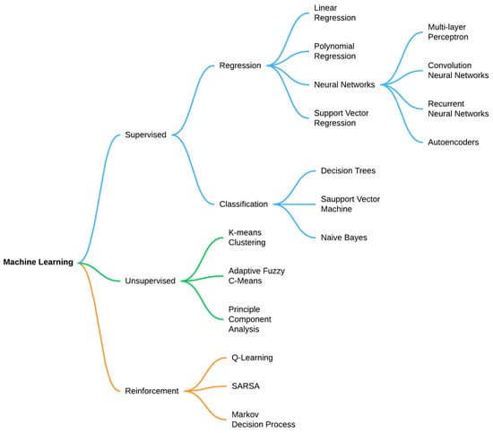
Figure 1.
Machine learning algorithms.
This review is an effort to highlight the different applications and machine learning (ML) techniques in coastal engineering. Several ML algorithms are employed as data-driven techniques in coastal applications. Commonly used algorithms are artificial neural networks (ANNs), Bayesian networks (BNs), decision trees (DTs), and support vector machines (SVMs). Detailed explanations of the different ML algorithms are available in numerous references e.g., [18,19], eliminating the need to give a comprehensive discussion here.
The inclusion of ML models in coastal engineering was mainly applied in three areas: wave field prediction, sea level rise, and morphology change. However, ML applications were also seen in other maritime engineering domains such as tsunamis [20,21,22], scouring [23,24,25], and breakwater design [26,27,28]. Despite the significance of these areas, extending this review to include all maritime applications would make this review work overly lengthy.
Section 2 provides a brief introduction to ML algorithms applied in coastal engineering. Previous studies for each application in the three areas are reviewed in Section 3. Section 4 presents and discusses the obtained results of this comprehensive review. Section 5 addresses the challenges facing scientists in applying AI methods in coastal engineering. Final thoughts are presented in Section 6. This endeavor aims to comprehensively assess the current landscape of ML applications in coastal engineering. While the initial goal was to examine research from 2015 onwards, it was often found that setting the context by incorporating earlier studies would be beneficial to the reader. This approach ensures a more holistic understanding of the evolution of these topics.
2. Machine Learning Tools Used in Coastal Engineering
2.1. Artificial Neural Networks
ANNs are the most commonly used ML algorithm in coastal engineering applications, being adaptable to different states and problems. The effectiveness of ANNs arises from their ability to model complex nonlinear problems, and therefore they have already been successfully used in tasks for classification and regression. Several ANN variations exist. In coastal engineering research, the frequently used neural networks are multi-layer perceptron (MLP), convolutional neural networks, and long short-term neural networks. Lecun et al. [14] and Juan and Valdecantos [29] present a detailed review of these variations. The MLP is the most commonly used and contains an input layer, one or more hidden layers, and an output layer (Figure 2). Each layer consists of nodes that are connected to the nodes of the previous and subsequent layers via a transfer function. Input layer nodes represent the independent variables, and usually each node represents one variable. Likewise, the output layer nodes represent the sought output variables. The number of hidden layers and their nodes are determined subjectively or through some sort of systematic analysis where multiple configurations are tried and the best combination is chosen. As data are passed from the input nodes to the subsequent layers, they are altered by transfer functions. Table 1 presents the commonly used transfer functions in coastal and ocean engineering [29]. Nodes are connected with the response function h as follows:
where is the input of the ith nodes, is the response of the jth neuron, is a bias constant, is the weight factor between and , and f is the transfer function. The weights and biases constants are found through optimization routines applied to the training dataset by backpropagating the errors from the output layer through the network and adjusting these constants.
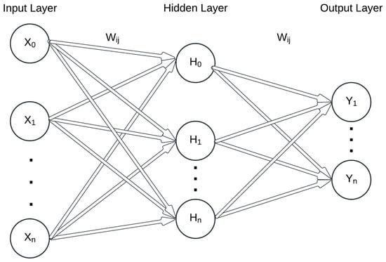
Figure 2.
Typical structure of the artificial neural network.

Table 1.
Transfer functions commonly used in ocean engineering [29].
2.2. Regression Tree
Regression trees use a binary split technique of the dataset to map a given feature to its targeted outcome. The split is recursively applied until a stopping criterion is met. Hastie et al. [30] advise growing a large tree with many splits and then pruning the tree (collapsing some splits) based on cross-validation and cost complexity. Trees are usually used for classification problems and have been used in coastal engineering problems in context with other ML techniques (e.g., [31,32,33]). The tree structure is visually appealing and aids in interpreting the paths to which the prediction is made, therefore making it easier to identify errors in the model. Input features of the regression tree can be of any type and have different scales. Nonetheless, small variations in the training dataset can result in different split schemes, thus decreasing the accuracy of the prediction and introducing uncertainty [34]. Different algorithms can be used to improve the accuracy of the regression trees. Bagging, boosting, and stacking are among the techniques used to build several models and then merge the results to decrease the uncertainty and improve the accuracy [34].
2.3. Bayesian Networks
Bayesian networks (BNs) are graphical representations of the probabilistic distributions between variables. BNs link the conditional probabilities of causal variables to their predicted outcomes explicitly. The structure of a BN is composed of nodes representing the variables and arrows between them representing the statistical connection forming an acyclic graph. For example, Figure 3 is an illustration of a BN for three factors that contribute to beach erosion volume [35]. In BNs, interactions between variables are clear, unlike in other ML techniques. This eases visualization and interpretation of the processes involved [36]. An advantage of using BN is that uncertainties can be estimated more accurately since probabilities are propagated through the network over all states. This is particularly important in the environmental modeling of nonlinear systems that contain uncertainties or risks [37]. However, the BNs have limited ability to model continuous data. This is a major limitation because nearly all data in environmental sciences are characterized as continuous. This instigates the need to discretize the variables. Beuzen et al. [35] compare three approaches for data discretization: manual, supervised, and unsupervised. Results indicate that the supervised approach produces the highest predictive skill.
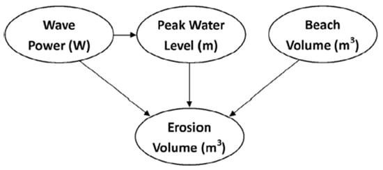
Figure 3.
Bayesian network for coastal erosion. Reprinted with permission from Ref. [35]. Copyright 2018, Elsevier.
2.4. Support Vector Machine
A support vector machine (SVM) is a supervised ML algorithm used for classification and regression tasks. The algorithm’s ability to handle high-dimensional data and its versatility make it a powerful tool in ML applications. In the context of classification, the SVM aims to find a hyperplane in a high-dimensional space that distinctly separates data points of different classes. In regression tasks, the goal is to predict a continuous outcome instead of assigning data points to classes. The data points that are crucial in defining the hyperplane are called support vectors. The hyperplane is chosen to have the maximum margin or separation, which is the distance between the hyperplane and the nearest data point of either class. Figure 4 displays the support vectors as the boundary lines separating the points. After the hyperplane has been found, the model function, displayed below, is used to give the classification decision.
where is the support vector weights, determined during the training process; and are the input and output vectors; is the kernel function; and b is a bias term. The SVM can employ several kernel functions to handle the nonlinearities of the data by transforming the input data into a higher dimensional feature space. Examples of kernel functions are linear, polynomial, sigmoid, and radial basis functions. For a detailed overview, refer to [38].
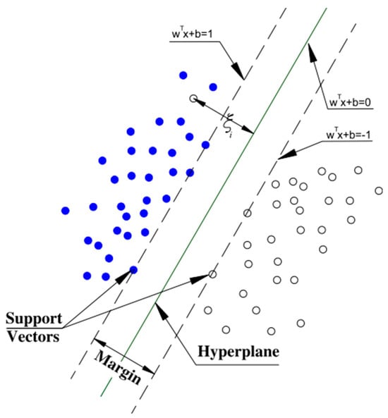
Figure 4.
Illustration of the support vectors and hyperplane to maximize margin. Reprinted with permission from Ref. [39]. Copyright 2011, Elsevier.
3. Application of ML in Coastal Engineering
Numerical models have long been the sought method for the simulation of coastal processes. Their accurate predictions and satisfying effectiveness led to their wide utilization in coastal engineering problems. Nonetheless, as models get larger and more complex, more computational resources and time are needed to handle the required computations. As such, scientists are often limited to applications of small spatiotemporal extent or are compelled to use certain assumptions to decrease the complexity of the model, thus abdicating the required precision.
The development of statistical techniques and the vast amount of collected data have given rise to ML tools as an alternative to traditional simulation methods. In many cases, ML techniques outperform traditional numerical methods [40,41,42]. Goldstein et al. [41] mentioned that this outperformance remains ambiguous. However, published results indicate a significant potential to widen the use of ML methods over numerical models.
A review of previous studies indicates that different ML techniques were successfully employed in a wide range of problems in coastal engineering. Nearly all studies displayed a slight to significant improvement in prediction skills over traditional methods. For example, Gracia et al. [43] studied the ability of MLP and decision trees to improve the accuracy of wave height modeling and achieved error reductions varying from 19% to 74%. Ellenson et al. [31] used the bagged regression tree method to predict and improve the error of the numerical wave model WAVEWATCH. The ML model was trained using field data and then was used to improve the numerical model wave prediction by 19% on average. Other enhancements attained a considerable decrease in required computational power and simulation time. One study [15] used a convolutional neural network to study nearshore processes and achieved a 22.5 times faster performance compared to the SWASH numerical model. Conversely, James et al. [16] applied a MLP neural network to study steady wave conditions and attained a performance 4000 times faster than the SWAN model.
Machine learning algorithms exploit past labeled data to infer relations between variables and thereby provide predictions. Inference from the data is solely dependent on the statistical distribution of the data and does not necessarily adhere to conservation laws. Therefore, training ML models requires a substantial amount of past data. Owing to the fact that the measured field data from beaches are scarce globally [1], scientists usually resort to generating training data using either numerical models or experiments. After the model is trained, it is validated using the existing field data. Figure 5 illustrates the process required in developing a ML model. Procedures such as selecting a suitable ML technique and the required number of input variables are of paramount importance and can significantly affect the performance of the model. The inclusion of more variables generally helps the ML model to capture the nonlinear relations and better represent a given process. However, one should take into consideration that too many variables can increase the potential of overfitting and consequently decrease the accuracy of the model [44]. Special care should be invested in deciding the input variables. Techniques such as principal component analysis, correlation, and clustering can help determine vital features. In the following sections, a synopsis of the use of ML in problems regarding wave modeling, water levels, and morphodynamics is provided.
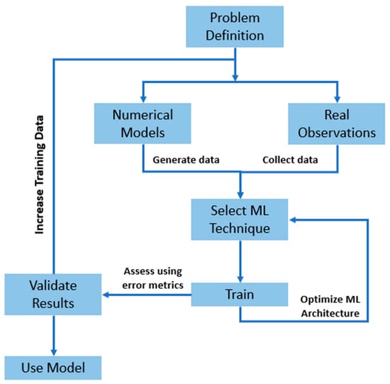
Figure 5.
Schematic illustration of the workflow required to develop a ML model [41].
3.1. Wave Field Prediction
Wave field predictions are very common in coastal and ocean engineering. The accurate prediction of wave characteristics is essential in many practical coastal engineering problems, such as understanding nearshore processes, monitoring beach profiles and shoreline changes, designing coastal protection structures, estimating potential wave overtopping risks, and evaluating environmental variables. Due to the complexity and the stochastic nature of waves, exact predictions are difficult [45]. Recently, data-driven models were used to overcome the sometimes imprecise and time-consuming numerical models and the costly deployment of in situ wave measurement equipment. A summary of research works on the application of ML techniques in wave modeling is presented in Table 2.
The development of ML models has followed different approaches. One possible classification can be based on the source of the dataset used for training. A widespread technique is to use data extracted from field measurements. This method is advantageous because it guarantees that the model will be trained on real case data, thus yielding a more accurate and better representative model. However, field data are often sparse and usually do not encompass a wide data distribution, which can result in a restricted model. Deo et al. [45] used an NN to predict significant wave heights and average wave periods based on inputs of wind speeds. The correlation between the observed and measured wave heights was found to be 0.77. Makarynskyy [40] instead investigated a three-layer NN to improve wave forecasting depending on previous values of wave heights and periods with a separate network for each. The author found smoother and more accurate representations for semi-enclosed sea rather than ocean water, which had more spatial and temporal variations. Decision trees were also used for wave height predictions. Mahjoobi and Etemad-Shahidi [46] applied a decision tree for significant wave height forecasting using wind speed and wind direction as inputs. The dataset used comprised 5-year measurements of wave heights and wind parameters. The study compared the performance of regression trees and ANNs on the same dataset. While error metrics slightly favored ANNs, the authors argued that the regression tree was effectively faster and required less time to build the model. In the same year, Günaydın [47] investigated the inclusion of more input parameters and compared the performance of seven ANNs to predict significant wave height. The author tested input combinations of meteorological data for wind speed, sea level pressure, and air temperature and found that the best performing ANN was the one including all data, with wind speed being the most influential.
Mahjoobi et al. [48] presented a comparison between ANNs, fuzzy inference systems (FISs), and adaptive neuro-fuzzy inference systems (ANFISs) in their ability to predict wave characteristics using inputs of wind speed, direction, fetch length, and duration. While the three models showed high prediction skills, it was found that the ANFIS was slightly more accurate than the other two. In 2011, Malekmohamadi et al. [39] carried out a similar endeavor where they compared the performance of four ML techniques to predict wave heights in Lake Superior, USA, based on records of wind speeds alone. They compared support vector machines (SVMs), Bayesian networks (BNs), ANNs, and ANFISs. Results indicate that ANNs, SVMs, and ANFISs provided similar accuracy with the ANN being slightly better, while the performance of the BN was unreliable. Analogous efforts were made by Berbić et al. [49], where they compared the performance of ANNs and SVMs to forecast significant wave heights for the next 5 h using inputs of past wave heights and wind. Both models generally showed equal accuracy; however, the SVM was slightly more accurate for shorter lead times, whereas the ANN was better for longer lead times. Kumar et al. [50] conducted a study to investigate the performance of two sequential neural network learning algorithms, namely the Minimal Resource Allocation Network (MRAN) and the Growing and Pruning Radial Basis Function (GAP-RBF), to forecast wave heights using measured inputs pertaining to location, month, wind, temperature, water depth, and previous wave heights. The performance of the MRAN and GAP-RBF were then compared with the support vector regression algorithm and the Extreme Learning Machine (ELM) and were found to be better in terms of accuracy. On the other hand, in 2022, a study was conducted to predict the occurrence of extreme wave heights using several ELM algorithms with meteorological inputs such as wind speed, direction sea level pressure, and air temperature [51]. The proposed technique first classifies extreme waves as outliers and other heights as normal. At that point, the ELM is trained on the detected outliers for classification. Results were then compared with other classification algorithms, such as logistic regression, decision trees, K-nearest neighbors, and MLP neural networks. It was found that the radial ELM method produced the most accurate predictions of all classifiers; nonetheless, it took a much longer run time compared to the other classification techniques.
Recently, Wei [52] undertook an intensive study to find the best amount of past input data needed to accurately forecast wave parameters. Wei developed a convolutional long-short-term memory (LSTM) model to predict three wave parameters: height, period, and direction with lead times of 1 h, 3 h, 6 h, 12 h, 24 h, and 48 h. Each lead time was further investigated with input to past data ratios of 1:1, 3:1, 5:1, and 7:1. The study included nine input parameters for waves, wind, temperature, and atmospheric pressure. It was concluded that the best predictions were obtained for shorter lead times with models having an input to past ratio of 1:1. Figure 6 shows that points representing bigger lead times are more dispersed around the line. The author clarifies that this behavior is probably caused by using a simple logistic function as the activation function, since it may not be sufficient to resolve the high nonlinearity in wave processes when the lead time increases. In the same year, Jörges et al. [53] designed an LSTM model for the time series prediction of wave heights considering bathymetric data. The inputs of the model were water levels, wind measurements, and a bathymetric transect of the research area of East Frisian Island in the German North Sea. It was found that the inclusion of bathymetry increased the performance of the LSTM by 16.7%.
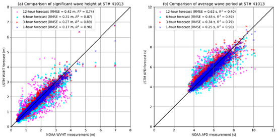
Figure 6.
Comparison of wave heights and wave periods for different lead times. Reprinted with permission from Ref. [52]. Copyright 2021, Elsevier.
Nowcasting waves based on collected data from fixed devices such as accelerometers also showed potential in wave characteristic estimates. Liu et al. [54] presented a one-dimensional convolutional NN to estimate wave height and period from acceleration data from accelerometers fixed on buoys. The approach statistically correlates acceleration data to sea surface movements and outperforms the traditional numerical method of converting acceleration into wave characteristics. Despite their novel methodology, the model was not applied to real conditions. Continuing on the previous approach, Demetriou et al. [32] proposed a method for the estimation of significant wave heights by monitoring meteorological data and the structural acceleration response of coastal structures. They developed an ANN and decision tree ensembles to use the inputs of accelerometers fixed on the bottom of a coastal jetty, together with wind speeds and direction, to nowcast incident significant waves on the jetty (Figure 7). The study presents a novel method to exploit the large number of existing structures by deploying monitoring devices onto them for real-time estimation of impacting waves.
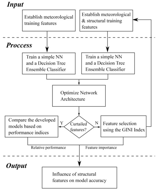
Figure 7.
Flowchart of the adopted methodology of accelerometers on jetty. Reprinted with permission from Ref. [32]. Copyright 2021, Elsevier.
Ma et al. [55] investigated the performance of an ANN wave prediction model under unknown seas. The ANN model was trained using a wave time series generated from experimental wave tank tests. The experiment considered four sea states with different significant wave heights and periods generated considering the JONSWAP spectrum. The ANN model used consists of an input layer, three hidden layers, and an output layer following the structure used by Duan et al. [56]. The input layer receives the wave heights of a measured position and the output layer outputs the heights of a predicted position. First, the ANN model was trained and tested on each sea state to measure its prediction accuracy. The results displayed high accuracy with errors < 6%. The second step was training the ANN model on one sea state and then using it to predict the wave heights of the other three sea states. Training and testing the model on different sea states significantly increased the error, which reached 24%. Ma et al. [55] mention that this poor performance was caused by the varying data distribution of the different sea states owing to the misprediction of the model. To rectify this behavior, the authors resorted to using a mixed sea state dataset to decrease the effect of varying data distribution, and the prediction ability improved (errors of 15% under different sea states). It is suspected that the model could be further improved if it were trained on additional features such as wave periods, wave direction, and wind characteristics.
Several other research studies have been conducted on the same flow path; however, the availability of field data was the major barrier. Therefore, many researchers shifted to using existing numerical models to generate data for model training and validation. Combining ML and numerical models was used extensively. Malekmohamadi et al. [57] generated artificial wind data to generate wave data using the WAVEWATCH3 model. The authors argued that the ANN can capture the relations between wind and wave and can thus be used for long-term wave estimation using real wind.
James et al. [16] developed a multi-layer perceptron model to simulate significant wave height in Monterey Bay California, USA. The goal was to train the model by generating data from simulations of the physics-based model SWAN based on historic wave, current, and wind data. The developed model accurately replicated the wave conditions in the domain and ran 4000 times faster than the SWAN model. In 2019, O’Donncha et al. [58] argued that aggregating an ensemble of simulations using perturbed inputs into the SWAN model can improve accuracy by transitioning from deterministic into probabilistic forecasting by considering the uncertainties in the forcing data. It was found that using the ridge regression aggregation decreased the error by 47% compared to the single forecasting model.
Wang et al. [59] proposed a composite physics-informed neural network model (PINN) to simulate wave fields using limited wave data generated from Xbeach and wave tank experiments for training. The PINN model infuses the governing equations for wave energy balance and dispersion relation into the NN as a loss function. The model was also constrained against the wave heights and directions computed with Xbeach (focus on steady wave fields without forcing of wind or currents). The model was assessed on a uniform barred beach and a 3D circular shoal experiment and showed sufficient accuracy in reconstructing the entire wave field.
Wei and Davison [15] developed a convolutional neural network (CNN) model composed of 16 hidden layers that can study the unsteady nearshore processes varying both spatially and temporally. The model was trained on data generated from numerical simulations of the SWASH model in a laboratory setup. The experiment included several coastal processes, such as wave propagation, wave interaction with sand bars, wave–current interaction, and unsteady rip currents. The CNN model was applied for estimating three hydrodynamic parameters, namely the water surface elevation, cross-shore velocity, and longshore velocity, and trained with pairs; i.e., it was fed by present values of the hydrodynamic parameters and used to predict the next time frame. The model achieved significant accuracy with a 22.5-times-faster computation than the SWASH model.
Another widespread approach is to use ML models as a complement to the numerical models; i.e., the results of the numerical model are processed by the ML algorithm to improve their accuracy. This is achieved by using the numerical model output as input to the algorithm and the real observations as the targeted output (Figure 8). The downside of this approach is the slightly higher computational cost required for post processing. Chang et al. [60] improved the accuracy of predicting typhoon-induced waves using the MIKE-SW model and ANN. Two wind parameters were included in the study: the wind velocity field in the area, VNCEP, and the wind velocity of the typhoon, VRVM. Both winds were used in the simulation of wave fields using the MIKE-SW model. The resulting wave heights, HNCEP and HRVM, together with VNCEP and VRVM, were inputs to the NN. The network was trained against measured wave heights resulting from 25 typhoons. The proposed network had four input units, one hidden layer with nine neurons, and one output neuron predicting wave heights. O’Donncha et al. [61] investigated a wave forecasting ML ensemble model using simulations from the SWAN model. The proposed approach depends on generating an ensemble of wave predictions for the next 48 h by inputting a set of perturbed boundary conditions into the SWAN model. The resulting outputs were integrated with observations with a set of weights minimizing the difference between SWAN predictions and the observations. Likewise, Gracia et al. [43] achieved an average error reduction of 36% by applying an ensemble average between a multi-layer perceptron and gradient boosting decision tree. Their study is based on input variables found from numerical modeling, such as wave height, wave period, direction, current velocities, and time. These datasets are then to be trained against actual wave measurements from buoys to provide corrections to the numerical model.

Figure 8.
Workflow of increasing accuracy of numerical models through machine learning.
Other studies used ML to train on the error of numerical models and observations and then used this error to modify the numerical model output [31,62,63]. Makarynskyy [62] attempted to improve WAM model output using an NN. Differences between the WAM model and buoy observation time series were introduced as inputs to the NN, which in turn predicted in advance the error of the leading 3 h and subsequently subtracted from the WAM model for rectification. Results showed a considerable enhancement of WAM prediction accuracy without the need to change the model settings. Continuing on Makarynskyy’s work, Londhe et al. [63] developed an ANN to predict the error of wave heights estimated by numerical models 24 h ahead. The study proposed a methodology to decrease the error of the numerical model MIKE-SW by forecasting the error and then adding or subtracting it from the numerical model results. Inputs to the ANN were the previous nine-step error to predict the next error in 24 h. Results show that forecasts performed by the numerical model and then corrected by the ANN output error have a significant improvement compared to the numerical model alone. Also, Ellenson et al. [31] used the bagged regression tree method to predict the output error of the WAVEWATCH3 model. The inputs included significant wave height, mean wave direction, mean wave period, wind magnitude, and wind direction. The model was trained and tested on measurements from the U.S. West Coast in the period from 2012 to 2013. Results show an overall improved prediction of 19%. However, when applied to measurements from 2015, the model showed poor performance. This resulted because the correlation features of inputs used in 2012–2013 were different than in 2015, particularly in wind magnitude, which further emphasizes that ML algorithms generally do not perform well when asked to extrapolate beyond the scope of training data.
Table 2.
Studies using ML techniques in wave modeling.
Table 2.
Studies using ML techniques in wave modeling.
| Author | ML Method | Source of Data | No of Data | Training/Testing% | Performance Indicator * | Inputs | Outputs |
|---|---|---|---|---|---|---|---|
| Deo et al. [45] | MLP NN | Field measurements | 900 | 80/20 | R | Wind speed, duration, fetch | Wave height, period |
| Makarynskyy [40] | MLP NN | Field measurements | 30,072 | 67/33 | R, RMSE, SI | Wave height, period | Wave height, period |
| Makarynskyy [62] | MLP NN | WAM | N/A | 67/33 | RMSE, R, SI | Past wave height error, past period error | Wave height error, period error |
| Mahjoobi and Etemad-Shahidi [46] | Decision Tree | Field measurements | 13,243 | 76/24 | Bias, RMSE, SI | Wind speed, direction | Wave height |
| Mahjoobi et al. [48] | MLP NN, FIS, ANFIS | Field measurements | 937 | 65/35 | Bias, R, SI, MSE, MSRE | Wind speed, duration, fetch, direction | Wave height, period, direction |
| Günaydın [47] | MLP NN | Field measurements | N/A | 80/20 | R, MSE, MARE | Wind speed, sea level pressure, air temp | Wave height |
| Malekmohamadi et al. [57] | MLP NN | WAVEWATCH3 | N/A | N/A | R | Wind speed | Wave height, period |
| Malekmohamadi et al. [39] | SVM, BN, MLP NN, ANFIS | Field measurements | 399 | 86/14 | Bias, SI, RMSE, MRE, R | Wind speed | Wave height |
| Chang et al. [60] | MLP NN | MIKE_SW | 5479 | 76/24 | RMSE, R | Wind speeds, wave heights | Wave height |
| Londhe et al. [63] | MLP NN | MIKE_SW | N/A | 70/30 | R, RMSE, MAE, CE | Past wave height error, past period error | Wave height error, period error |
| Berbić et al. [49] | MLP NN, SVM | Field measurements | 13,140 | 65/35 | R, RMSE, RAE, MAE, RRSE | Past wave heights, wind speed | Wave height |
| Kumar et al. [50] | MRAN, GAP-RBF | Field measurements | 22,852 | 88/12 | R, RMSE | Latitude and longitude, wind speed, month, temperature, water depth, atmospheric pressure, past wave heights | Wave height |
| Kumar et al. [16] | MLP NN, SVM | SWAN | 11,078 | 90/10 | RMSE | Wave height, period, direction, wind speed, currents | Wave height, period |
| O’Donncha et al. [61] | MLP NN | SWAN | N/A | N/A | RMSE, MAPE | Perturbed inputs into SWAN | Wave height |
| O’Donncha et al. [58] | MLP NN | SWAN | 11,078 | 90/10 | MAPE | Perturbed inputs into SWAN | Wave height |
| Liu et al. [54] | CNN | Field measurements | 128 | 5-fold cross-validation | MAE, MSE | Buoy acceleration | Wave height, period |
| Duan et al. [56] | MLP NN | Wave tank experiment | N/A | N/A | RMSE, NDRMSE | Past wave heights | Wave heights |
| Ellenson et al. [31] | Regression Tree | WAVEWATCH3 | 20,250 | 60/40 | RMSE, Bias, SI, PI | Wave height, period, direction, wind speed, direction | Wave height error |
| Wei [52] | LSTM | Field measurements | 17,543 | 68/32 | RMSE, R2 | 9 parameters related to winds, waves, temp, atmospheric pressure | Wave height, period, direction |
| Wei [53] | LSTM | Field measurements | 7929 | 47/53 | RMSE, MAE, MAAPE, R, R2 | Water levels, wind speed, wind direction, bathymetric transects | Wave height |
| Demetriou et al. [32] | MLP NN, Decision Tree | Field measurements | 51,444 | 70/30 | Accuracy, Markedness, Fscore, Kappa statistic | Wind speed, direction, jetty acceleration | Wave height |
| Ma et al. [55] | MLP NN | Wave tank experiment | 10,000 | 80/20 | RMSE, NDRMSE | Past wave heights | Wave heights |
| Gracia et al. [43] | MLP NN, Decision Tree | N/A | 97,483 | 80/20 | MAE, R | Date, time, wave height, period, direction, wind speed, direction, currents | Wave height, period, direction |
| Mahmoodi and Nowruzi [51] | ELM | Field measurements | 5060 | 75/25 | Accuracy | Wind direction, wind speed, sea level pressure, air temp, water temp | Wave height |
| Wang et al. [59] | PINN | Xbeach/experiment | 126 | 50/50 | RMSE, R2 | Location, direction | Wave height, direction |
| Wei and Davison [15] | CNN | SWASH/experiment | 10,000 | 80/20 | MASE, R2 | Water surface elevation, cross-shore velocity, longshore velocity | Water surface elevation, cross-shore velocity, longshore velocity |
* Correlation coefficient (R); Root mean square error (RMSE); Mean absolute error (MAE); Mean square error (MSE); Mean relative error (MRE); Mean square relative error (MSRE); Mean absolute relative error (MARE); Scatter index (SI); Coefficient of efficiency (CE); Coefficient of determination (R2); Mean arctangent absolute percentage error (MAAPE); Persistency index (PI); Root relative square error (RRSE); Non-dimensional RMSE (NDRMSE).
3.2. Water-Level Fluctuations
Table 3 summarizes the main practices employed in surrogate modeling and forecasting of sea level fluctuations and storm surges. The objectives and algorithms used differ between those studies. The input features used varied between meteorological data, storm features, tidal components, astronomical variables, and past sea level measurements. Sztobryn [64] investigated the application of ANNs in surge forecasting using past inputs of sea levels. He concluded that ANN performance is comparable to traditional methods when a continuous input series is used for forecasting. Later, Lee [65,66] used input factors such as typhoon center pressure, wind speed, wind direction, and harmonic analysis of tidal levels and employed a backpropagation NN to predict the resulting storm surge levels for short lead times. In 2007, Tseng et al. [67] compared four MLP models with varying inputs to predict typhoon surge levels for short lead times of up to 3 h. The best model included 18 input parameters for typhoon characteristics and meteorological conditions for present and previous times. Rajasekaran et al. [68] used the same input parameters as Lee [65] to compare the performance of a finite-volume numerical model, neural network, and SVM regression. The study concluded that the SVM was superior in terms of accuracy and computational effort. On the other hand, a later study [69] found that SVMs and ANNs had similar accuracy when compared together to predict the surge level due to tropical storms. The models were trained using 1026 synthetic storms simulated on multiple software such as WAM, STWAVE, and ADCIRC. The performance of SVMs and ANNs were similar except that the ANN was better at predicting extreme events. The study also investigated the minimum number of data needed for model training, which was found to be at least 300 storms for an acceptable accuracy.
Jia and Taflanidis [70] used a Kriging model to predict storm surges and wave heights at a large geographical area around the islands of Hawaii with a real-time risk assessment. The study utilized synthetic training data from numerical models and used principal component analysis (PCA) to decrease the number of output points and improve computational efficiency. This is performed under the assumption of spatial and temporal correlation between the output points. The study demonstrated that using PCA to decrease output dimensionality significantly reduced memory demands but with a slight decrease in accuracy. Furthermore, a comparison between the Kriging model and moving least squares response [71] showed a similar performance in terms of accuracy but a favorable computational efficiency for the Kriging model. Subsequently, Kim et al. [72] developed an ANN to predict a time-dependent storm surge and storm inundation estimation in advance of storm landfall. The study showed that the surrogate model accurately forecasted a time-series of storm surges before landfall; however, accuracy decreased after storm landfall. Also, a decrease in accuracy was found at inland locations where complex structures were found, such as inland marshes and lakes. In advance of the previous studies, Jia et al. [73] examined the Kriging surrogate model combined with PCA to provide an accurate real-time time series and peak surge levels with reduced computational resources. The study included a correction stage to address dry/wet nodes during some storms. Later, Lee et al. [74] designed a new surrogate model to predict peak storm surges in coastal regions by employing tropical cyclone track time series. The model depends on a one-dimensional convolution neural network for the consideration of the track time series and consists of K-means clustering and PCA to increase computational efficiency. The authors trained the model with 1031 synthetic storms, including landfalling and bypassing storms to consider all possible sources of surges.
Bass and Bedient [75] developed a surrogate model to predict the combined effect of rainfall runoff and peak storm surges resulting from tropical storms over a wide coastal area. They utilized the outputs of numerical models of 223 synthetic storms to provide joint surge estimates and probabilistic distribution in the watershed area. The study also compared the performance between an ANN and Kriging model and showed that the latter was more accurate. The authors state that the Kriging model is better suited to learning spatial information since it considers the covariance between input features and the output. Another comparative study was carried out to assess the performance of ANN, Kriging, and support vector regression models [76] on tropical storm surge prediction. Although it was evident that the target surge height can significantly affect the accuracy of the surrogate model, ANN and Kriging models showed a consistent performance in contrast to the SVR method. The Kriging method also displayed consistent conduct and accuracy when trained with a small dataset, as opposed to the ANN and SVR.
Riazi [77] used an NN for tidal level estimation. The network has four input neurons, three for astronomical factors and one for geology, geomorphology, and biological factors combined. Although this study takes into consideration the effect of geomorphological factors, their inclusion is only limited to one input value and is calculated as a bias term to adjust the tidal levels in the model. The author used a genetic algorithm to obtain the value of this neuron weight. Compared to a set of recorded tidal levels at six locations, the model showed a reliable and accurate performance, even though the effect of sea level rise was neglected. Similarly, Ishida et al. [78] used astronomical features such as moon and sun positions, along with other variables, to estimate an hourly time series of sea level change taking into consideration the effect of global warming on the sea level. The study was conducted by an LSTM NN and applied to a dataset of 39 years. The model showed that it could accurately predict hourly fluctuations along with the timings of monthly fluctuations; however, peak values of sea levels were underestimated. Alternatively, Accarino et al. [79] relied on previous time series of sea levels to give a three-day prediction at specific locations using LSTM. The authors employed a multimodal LSTM in which two independent networks were used. Each network was trained with different time steps in the time series and used to predict the following three days. Then outputs of both models were concatenated to obtain the best accuracy. Although it was shown that the prediction quality decreased for the later days, the multimodal LSTM performed better when compared to the SANIFS forecast model. Guillou and Chapalain [33] compared the performance of multiple regression methods based on linear and polynomial functions and an artificial neural network (ANN) for the prediction of water levels in the Elorn estuary in Landerneau, France. Input variables considered were French tidal coefficients, atmospheric pressure at mean sea level, wind velocity, and river discharge. The model was trained against successive high tides. Results show that the best estimates were predicted for the multiple polynomial regression of the second degree and the multi-layer perceptron with three hidden layers and five neurons per layer.
Additionally, multiple efforts were undertaken to increase the accuracy of the developed surrogate models. Zhang et al. [80] developed a systematic methodology to assess the addition of new synthetic storms for model training to increase the forecasting accuracy. The study employed a Kriging model for storm surge estimation. An adaptive selection procedure was used to identify storms whose addition to the training dataset would likely increase the prediction accuracy using the least number of synthetic storms, thus increasing computational efficiency. This selection procedure is accomplished iteratively, where new storms are tested and the Kriging model is retuned and evaluated. The study also addressed storm intensification and sea level rise for future extrapolation by giving larger weights to more intense storms. Kim et al. [81] proposed a methodology to systematically select the best parameters to develop a NN for sea level forecasting. The objective of their study was to determine the best-performing model by changing the combination of input parameters and the number of hidden units in a single hidden layer. The inputs were combined into 12 combination sets. Several models were developed for each set of inputs based on varying hidden units and randomized weights and biases between the units. A total of 957 models were explored to settle on the best performing model to predict 5, 12, and 24 h lead forecasting times. Although the authors mentioned that their procedure is novel, their technique is a brute force method. More recently, Kyprioti et al. [82] found that parameterizing the inputs to the nearest point to the domain of interest instead of landfall as a reference point could be a better representation and increase model accuracy. The study also investigated the concern of overfitting as a result of limited training instances. They maintained that a parametric analysis should be performed to measure the model accuracy given the number of retained variables, especially when using principal component analysis.
Table 3.
Studies using ML techniques in sea level modeling.
Table 3.
Studies using ML techniques in sea level modeling.
| Author | ML Method | Source of Data | No of Data | Training/Testing % | Performance Indicator * | Inputs | Outputs |
|---|---|---|---|---|---|---|---|
| Sztobryn [64] | MLP NN | Field measurements | N/A | N/A | R, RMSE | Sea levels, wind speed, direction | Storm surge elevation |
| Lee [65] | MLP NN | Field measurements | N/A | N/A | R, RMSE | typhoon center pressure, wind speed, wind direction, and harmonic analysis of tidal | Storm surge elevation |
| Tseng et al. [67] | MLP NN | Field measurements | 16 | 75/25 | R, CE, error of surge peak, error of peak time | 5 typhoon characteristics and 4 meteorological conditions for present and previous times | Storm surge elevation |
| Lee [66] | MLP NN | Field measurements | N/A | 50/50 | R, RMSE | Typhoon center pressure, wind speed, wind direction, and harmonic analysis of tidal | Storm surge elevation |
| Rajasekaran et al. [68] | MLP NN, SVM | Field measurements | 72 | 50/50 | RMSE | Typhoon center pressure, wind speed, wind direction, and harmonic analysis of tidal | Storm surge elevation |
| Jia and Taflanidis [70] | Kriging | ADCIRC, SWAN | 563 | 70/30 | R2, AME | Landfall location, angle of landfall, central pressure, forward speed, radius of max wind, tide level | Storm surge elevation, wave height |
| Kim et al. [72] | MLP NN | ADCIRC, STWAVE | 446 | 70/30 | R, MSE | Latitude and longitude, heading direction, central pressure, forward speed, radius to max wind | Storm surge elevation |
| Jia et al. [73] | Kriging | ADCIRC, STWAVE | 446 | Leave-one-out cross-validation | R2, AME, AMSE | Latitude and longitude, heading direction, central pressure, forward speed, radius to max wind | Storm surge elevation |
| Hashemi et al. [69] | MLP NN, SVM | NACCS’s model | 70/30 | MSE, R | Central pressure, wind radius, forward velocity, storm track | Storm surge elevation | |
| Bass and Bedient [75] | MLP NN, Kriging | HEC-HMS, HEC-RAS, ADCIRC, SWAN | 223 | 10-fold cross-validation | R2, RMSE, AME | Central pressure, radius to max wind, forward speed, angle of approach, longitude | Joint rainfall flooding + storm surge |
| Zhang et al. [80] | Kriging | ADCIRC, STWAVE | 595 | Leave-one-out cross-validation | R, R2, RMSE | Latitude and longitude, heading direction, central pressure, forward speed, radius to max wind | Storm surge elevation |
| Kim et al. [81] | MLP NN | Field measurements | 460 | 75/25 | R, NRMSE | surge level, sea level pressure, drop of sea level pressure, wind speed, wind direction, central pressure, longitude and latitude | Storm surge elevation |
| Al Kajbaf and Bensi [76] | MLP NN, Kriging, SVR | ADCIRC | 1031 | 70/30 | R, RMSE, MSE, MAE | Latitude and longitude, heading direction, central pressure, forward speed, radius to max wind | Storm surge elevation |
| Ishida et al. [78] | LSTM | ERA5 dataset | N/A | 67/33 | RMSE, NSE | Wind speed, wind direction, mean sea level pressure, air temperature, and four variables of moon and sun position | Sea level |
| Riazi [77] | MLP NN | Field measurements | 130,584 | 71.6/28.4 | MSE | Moon position, Earth position and rotation, geology and geomorphology factors | Tide level |
| Kyprioti et al. [82] | Kriging | ADCIRC | 156 | Leave-one-out cross-validation | NRMSE, misclassification index, surge score | Latitude and longitude, heading direction, central pressure, forward speed, radius to max wind | Storm surge elevation |
| Accarino et al. [79] | LSTM | Field measurements | N/A | 80/20 | R2, RMSE | Past sea levels | Sea level |
| Guillou and Chapalain [33] | Multiple regression, MLP NN | Field measurements | 1536 | 70/30 | MAE, RMSE, R2 | French tidal coefficients, atmospheric pressure, wind velocity, river discharge | Sea level |
| Lee et al. [74] | CNN | ADCIRC, STWAVE | 1031 | 10-fold cross validation | RMSE, mean bias error | Latitude, longitude, heading direction, central pressure, radius of maximum winds, translation speed | Storm surge elevation |
* Correlation Coeff. (R); Root mean square error (RMSE); Mean square error (MSE); Absolute mean error (AME); Coeff. of determination (R2).
3.3. Morphology Change
The ML algorithms were also used extensively in the field of sediment transport and morphological changes. As with previous cases of wave and water-level variability studies, the availability and increase in collected datasets paved the way for scientists to engage with ML in coastal sediment studies. The motivation is to provide a more reliable and accurate predictor, substituting the long computational hours demanded by the morphological models.
Applications such as sediment transport rates, sediment properties, morphological changes of beach profiles and shoreline, and integration of ML in physics-based numerical models were all investigated and showed promising, if not superior, results compared to the traditional techniques. Goldstein et al. [41] comprehensively reviewed the ML models currently used in coastal sediment transport and morphodynamics. The review mentions research applications in sediment transport, morphology models, and hybrid morphological models. The reader is certainly advised to review this article for more insights.
Since then, numerous research studies have been performed in line with the previously mentioned topics that highlight the capabilities and reliability that these models have set forth since their synthesis. A summary of these studies is presented in Table 4. Shafaghat and Dezvareh [83] used an SVM for classification and regression of sediment transport rates measured from the coasts of Hormozgan province in Iran. The optimization of SVM parameters was carried out using the RBF kernel, resulting in better accuracy than the linear and polynomial kernels. The authors further investigated the results of Kamphuis’s empirical equations [84,85] and compared them with the performance of the SVM and MLP models. It was found that the Kamphuis equations produced an overestimated transport rate, while the SVM and the MLP models were more accurate. Although the SVM and the MLP models had marginal differences, the authors mention that using an SVM is preferable because it requires less training time. Additionally, in cases of limited datasets, an SVM can often perform better than an MLP, which needs large datasets for parameter fitting [86]. Similar results were found in an earlier study [87] in which they implemented the same models and found that the SVM was 4% more accurate than the MLP in reproducing sediment transport rates.
Phillip et al. [88] developed an ensemble ML method called Bayesian Optimal Model System based on staking multiple algorithms [89] into one system where the final output is a probabilistic estimation of the ripple wavelength. The system is based on two ML algorithms, Gradient Boosting Regressor and XGBoost Regressor, and two empirical equations adopted from [5,90]. Their output is then passed to a Bayesian Linear Regression model that computes the posterior probabilistic distribution of the ripple wavelengths. The study utilized a dataset of more than 50 years compiled through field and laboratory studies of wave-induced ripples. The developed system provided better predictions than each independent base model alone. Previously, Goldstein et al. [91] used a similar dataset for wave ripple prediction. They used genetic programming to estimate the ripple wavelength, height, and steepness under the action of waves. Most notably, the authors employed a maximum dissimilarity algorithm to select the most dissimilar centroids of the data, representing the variance in the dataset. This results in minimum training data while leaving most of the data points available for testing and validation. Employing this technique allowed the authors to use only 6% of the data for training, incredibly less than any other study.
The determination of suspended sediment concentration was also explored using data-based/artificial intelligence techniques. Makarynskyy et al. [92] used an ANN to combine the modeling of waves and hydrodynamics with measured suspended sediment concentrations. The HYDROMAP and SWAN models were used to calculate the parameters of waves and hydrodynamics using tides and waves. Suspended sediment concentrations from two different sites were then combined to train the model. Although results were promising, this model was site-specific due to underlying assumptions and narrow data range. Zhang et al. [93] also explored suspended sediment concentration by comparing multiple data-driven techniques. They implemented the least absolute shrinkage and selection operator (LASSO) with a proposed temporal correlation on a large dataset for the Bohai Sea in China, taking into consideration hydrodynamic parameters to give 1-h forecasts. The performance of the LASSO model was then compared with classification and regression tree (CART), SVR, and MLP. Although the LASSO technique had the best accuracy, the differences between the models were nominal. However, incorporating a one-order autocorrelation for the suspended sediment concentration resulted in an improved accuracy for all the methods studied. Stachurska et al. [94] also investigated the CART method for the determination of non-cohesive sediment velocity. The purpose was to determine the wave-induced sandy sediment velocity over a rippled beach by incorporating the outcome of particle image velocimeter and conditional characteristics regarding waves and bed morphology. The authors employed two metaheuristic methods, PSO and SPBO, for parameter optimization. Running the meta-heuristic optimization increased computational time; however, it significantly increased the desired accuracy. They further made a comparison between CART and ANFIS for the accuracy of sediment velocity determination and concluded that the CART method was superior to the ANFIS method.
Bujak et al. [95], on the other hand, focused on the spatial variability rather than the temporal changes. The authors developed an MLP model to predict the required gravel nourishment volume along the Croatian shore. The study indirectly included the forcing of waves through the fetch length and beach orientation. It was found that among basic features such as beach area and length, fetch length had a significant effect on the ANN’s predictability. Nonetheless, the model displayed both overprediction and underprediction on several sites along the Croatian coast, with relatively high errors in some places; however, the authors argue that these errors are acceptable since they are within 10% of the required nourishment range. Another nourishment study investigated beach profile and erosion tendencies by using different nourishment techniques [96]. The study was undertaken in an experimental wave flume with four cases of nourishment, each with two sea levels. The results of the experiments were then fed to a backpropagation NN to replicate the results. Nonetheless, the results of the ANN were not significant due to the limited available training data, which affirms the underlying limitation that ML is only effective with large datasets. Conversely, Kumar and Leonardi [97] trained an ensemble of NNs on more than 500 Delft3D simulations to apply mega-nourishment projects, otherwise known as sand engines, in Morecambe Bay, UK. The purpose was to develop a decision support system with optimized modeling to provide an operational framework for the assessment of sand engines and evaluate their effects on the nourished area. The authors used an ensemble of eight ANN models combining both Recurrent Neural Networks and Feed-Forward Neural Networks. They utilized simulations from Delft3D with varying sand engine designs and fed them to the ML ensemble for the mean and maximum prediction of water depth, wave height, and sediment transport both before and after the nourishment.
Similarly, Simmons and Splinter [9] utilized a large dataset of 39-year beach transects on the Sydney coastline to compare different modeling approaches in simulating storm-induced erosion. They compared the errors of an empirical model developed by Harley et al. [98], the SBEACH numerical model, the XBEACH numerical model, and an MLP neural network model. The performance of each model was assessed based on the beach dataset composed of moderate to large storm events. While the MLP model had the best accuracy among the four models, an ensemble method of averaged weights of the four models provided the best skill across all storms studied and the most accurate performance above any separate model. On the other hand, Melo et al. [99] attempted to solve a full 2D morphological domain, not just transects, by replicating the morphological evolution of complex coasts involving a groin and a breakwater by using a hybrid technique. To reduce the computational cost of Xbeach to compute morphological evolution, the authors developed an emulator of the morphological module capable of reproducing images of current and cumulative bed level changes. Images of hydrodynamic numerical simulations were fed into the network for morphology computation. The network architecture, adapted from Melo et al. [100], is composed of U-nets and recursively deconvolutional branched networks to map the features of input images. These input images were the discretized spatial domain of mean velocity and bed shear stresses resulting from the hydrodynamic simulation. The resulting hybrid technique reduced the overall simulation time by 23% for a high-resolution domain and 87% for a low-resolution domain, indicating that the hydrodynamic simulation had the most restrictions for the performance gain. The results of the morphology network were very promising. Nonetheless, cases of erosion underestimation were found near the groin structure. The authors relate these errors to the lack of sufficient training instances.
Santos et al. [101] attempted to study the dune changes on Dauphin Island, northern Gulf of Mexico, during storms using statistical methods. They implemented synthetic storm generation following Wahl et al. [102] and used the 2D Xbeach model to generate the training cases for the surrogate models with varying storm conditions. Multiple Linear Regression, ANN, Random Forest, and Multivariate Adaptive Regression Spline (MARS) methods were all trained on the storm conditions and the post-storm profiles of 200 transects along the island’s coast. The ANN and MARS showed comparable and superior performance across all the cases, proving that these models can indeed act as surrogates for the physics-based models. However, the performance of the developed ANN and MARS were bound by the pre-storm profile, making their application site-specific. Athanasiou et al. [103] attempted to overcome this localized issue by incorporating a pre-storm nearshore slope as an input to the ANN. They trained the ANN on profiles simulated from the 1D Xbeach model. The inputs to the ANN were a combination of pre-storm conditions, waves and morphology, and storm conditions. Although the study realized some simplifying assumptions such as a 1D model, shore-normal waves, and sediment size, the inclusion of pre-storm morphological conditions increased the prediction accuracy of the model to 94% in terms of detecting erosion occurrence, with a skill score of 0.82 in estimating erosion quantity, and arguably did not restrict the model to a specific location. Itzkin et al. [104] also studied dune morphology by using an NN in conjunction with a genetic algorithm to optimize the calibration process of the Windsurf model. The Windsurf model would then produce a set of hindcasts upon which an LSTM neural network would use, along with associated forces such as waves, tide, and wind, to produce a 5-year forecasting of dune morphology. This work frame improved the calibration process used to generate training instances for the LSTM. As such, the LSTM was shown to predict the dune changes with good accuracy when the changes were close. Nonetheless, the model’s performance was lacking when it attempted to forecast an “out of sample” instance, such as Hurricane Florence. This behavior confirms the widely accepted consensus that ML methods do not extrapolate well out of the range [41,105].
Perhaps one of the most comprehensive studies performed in this regard was by Montaño et al. [106]. They carried out a contest of 19 different models to test their ability to predict shoreline changes. The models were a mixture of traditional models relating to different formulations of equilibrium transport rates and ML models, such as MLP, LSTM, Bayesian networks, K-nearest neighbors, and Random Forests. The aim was to test each model performance on 18 years (1999–2017) of daily averaged shoreline position in Tairua beach, New Zealand. The models were trained and validated on data from years 1999 to 2014 and then tested on the remaining three consecutive years. It was found that almost all models captured shoreline oscillations that happened on the order of 3 months. Traditional models had a smoother prediction trend than ML, meaning that they often underestimated extreme erosion events. ML techniques, on the other hand, were capable of detecting sudden erosion/accretion events not captured by traditional models. However, these ML models were more susceptible to other localized errors. In this regard, both modeling approaches complement each other owing to the inductive/deductive nature of the ML and traditional models, respectively. The authors concluded that an ensemble method, combining both approaches, produces the best accuracy compared to any single model. This conclusion was also shared by previously mentioned studies [9,58,61,88,97].
Table 4.
Studies using ML techniques in morphodynamics modeling.
Table 4.
Studies using ML techniques in morphodynamics modeling.
| Author | ML Method | Source of Data | No of Data | Training/Testing % | Performance Indicator * | Inputs | Outputs |
|---|---|---|---|---|---|---|---|
| Goldstein et al. [91] | Genetic Programming | Field measurements, Experiments | 995 | 6/94 | NRMSE, R | D50, mean wave period, wave amplitude, water depth | Suspended sediment concentration |
| Makarynskyy et al. [92] | MLP NN | Field measurements, HYDROMAP, SWAN | 1059 | 75/25 | NRMSE, MRE | Suspended sediment concentration, current velocity, wave height, period, direction, bottom wave orbital velocity | Suspended sediment concentration |
| Santos et al. [101] | MLRM, MARS, MLP NN, Random Forest | XBeach | 20,000 | 70/30 | R, RMSE, STD | Significant wave height, wave period, direction, tide level, total water level | Dune toe elevation, crest elevation, area across cross profile, barrier island width, dune toe location, dune crest location |
| Dezvareh and Shafaghat [87] | SVM, MLP NN | Field measurements, LITDRIFT | 32,949 | 90/10 | R2, RMSE | Wave height, period, direction, sediment size | Sediment transport rate |
| Montaño et al. [106] | MLP NN, LSTM, BNN, K-NN, RF | Field measurements | 18 years of daily frequency | N/A | R2, RMSE, skill | N/A | Shoreline position |
| Bujak et al. [95] | MLP NN | Field measurements | 228 | 70/30 | MSE | Beach area, beach length, beach orientation, fetch length, gravel size, wind intensity, tidal range | Nourishment volume |
| Kim and Aoki [96] | MLP NN | Experiments | 8 | 75/25 | RMSE, MAE, MSE | Cross-shore distance, initial profile, time, height, period, case, sea water level | Change of profile |
| Shafaghat and Dezvareh [83] | SVM, MLP NN | Field measurements | 63,360 | 90/10 | R2 | Wave height, period, direction, sediment size | Sediment transport rate |
| Zhang et al. [93] | LASSO, CART, SVR, MLP NN | Field measurements | N/A | 10 fold cross validation | RMSE, MAE | Water depth, flow speed, wind speed, wave height, wave period | Suspended sediment concentration |
| Athanasiou et al. [103] | MLP NN | XBeach | 12,540 | 80/20 | Skill score, Bias, RMSE, Mielke index | Max dune volume, beach volume, beach width, beach slope, nearshore slope, wave height, period, wave energy, storm surge level, angle of incidence, mean high water level | Dune erosion volume |
| Itzkin et al. [104] | MLP NN, LSTM | Field measurements, Windsurf | 2783 | 60/40 | RMSE, BSS | Vegetation friction, vegetation density, Aeolian transport coeff., wave asymmetry, wave skewness, critical slope, bed friction coeff., alongshore transport gradient | Dune crest height, dune toe elevation |
| Phillip et al. [88] | Gradient Boosting Regressor, XGBoost, Bayesian Regression | Field measurements, Experiments | 3499 | 10 fold cross validation | R2, RMSE, Bias | Grain size, wave period, water depth, semi-orbital excursion, ripple height | Ripple wavelength |
| Simmons and Splinter [9] | MLP NN | Field measurements | N/A | Cross-validation | NMSE | Wave height, wave direction, wave period, wave power, wave runup, impact hours, astronomical water level, storm duration, pre-storm beach width, beach volume, beach slope | Change in beach width, erosion volume |
| Stachurska et al. [94] | CART, ANFIS | Experiments | 1200 | 85/15 | RMSE, R2, NSE | Wave period, wave height, ripple length, ripple height, thickness of bottom layer, | Sediment particle velocity |
| Melo et al. [99] | CNN | XBeach | 204 | 80/20 | RMSE, ME | Generalized Lagrangian mean velocity, bottom shear stress | Current bed level change, cumulative erosion, and sedimentation |
| Kumar and Leonardi [97] | RNN, MLP NN | Delft3D | 552 | 90/10 | Regression, MAE, STD | Sand engine height, sand engine radius, wave height, distance between sand engine and boundary, angle of coastline, depth average velocity | Water depth, wave height, sediment transport |
* Standard deviation (STD); Brier skill score (BSS); Normalized root mean square error (NRMSE); Mean error (ME).
4. Discussion
A variety of studies applying a range of ML tools in coastal engineering were examined, particularly in the subfields of wave modeling, water level fluctuations, and morphology change. It can be seen from the summary tables and Figure 9 that the most used ML method is the NN. Nearly 60% of the reviewed articles avail to NNs to resolve the relationship between inputs and the intended outputs. Clemente et al. [107] found a similar percentage when reviewing applications of ML in wave energy conversion. This could be due to the versatility of the NNs to detect implicit relationships between dependent and independent variables. Neural networks also generally require less training effort compared to other techniques [108,109], which can make them more appealing to researchers.
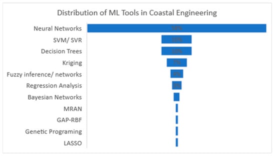
Figure 9.
Frequency of ML tools used in coastal engineering.
There are several types of NNs. This review identified five variations of NNs applied to the coastal engineering field. Figure 10 shows that the most commonly used variation among the reviewed articles was the MLP. Nearly three-quarters of the research that chose to work with NNs resorted to MLP. This could also be explained by the simplicity of the MLP compared to other types. Although LSTM, a type of RNN, showed great capability to model time-dependent processes, it accounted for only in one-tenth of the research. Despite the fact that this technique was formulated nearly three decades ago [110], its application to coastal engineering has only been seen recently and is expected to increase due to its memory-retaining capabilities, which makes it useful for temporal problems.

Figure 10.
Frequency of used types of NNs.
As model development depends highly on the quality of the past data used for training, it is imperative to use reliable data sources. Figure 11a summarizes the source of data used for model training. Nearly half of the articles used either field data alone or in conjunction with other data types. This majority is logical since researchers aim to train the ML models to mirror physical processes as accurately as possible, which means that these models should see the realistic historical trends of these processes. Data generated from numerical models were also used extensively, about 40% of the time. This was seen to be due to two reasons: (i) field measurements are generally harder to obtain, which motivates researchers to resort to established numerical models to generate sought data, and (ii) many of these articles aimed to partially or fully substitute the numerical models in certain aspects to increase computational speed, thus training the models on the same numerical output. Laboratory experiments, on the other hand, were not part of a significant number of studies. They neither fully reflect the realistic processes, nor do they stand to be substituted by other techniques. Given this understanding, it is expected that field measurements and numerically generated data are the main sources for model development. Figure 11b shows the combinations of utilized data sources. It is also clear here that the most used are the field and the numerical data alone. It was seen in the review that researchers would occasionally combine data from several sources to enlarge the training pool. However, only a small percentage of research resorted to combined data sources.

Figure 11.
Distribution of training data sources according to the literature. (a) Percentage of data types used to train the models. (b) Percentage of research utilizing combined data sources.
Looking at the quantity of data utilized by each study to train and validate the developed models, one can see a large variation in data instances among them. Figure 12 displays the total number of instances and the number of features used to develop the models in the reviewed research. Most studies ranged from 100 to 100,000 instances divided between training, validation, and testing. Given this high variability in training instances and the different performance-measuring metrics that were used among the reviewed articles, it is hard to pinpoint the exact impact that the quantity and quality of the utilized data had on accuracy. Most of these studies were limited by the available data. The determination of the required training size is highly dependent on the problem at hand and the sought accuracy. It is hard to map a relation between the number of variables and the required data to yield an acceptable accuracy for each case. It is generally acknowledged that more training data is beneficial for the development process since it gives the model a chance to learn from a wider spectrum. However, since acquiring substantial data is often a limiting issue, it is often a question of the minimum data needed to yield a noteworthy performance. In this case, special care should be given to improve the data quality, namely avoiding the presence of noise and outliers in the dataset. Nonetheless, this would raise the risk of overfitting [82,83]. Hashemi et al. [69], for example, concluded that at least 300 instances were needed to train their model for an acceptable precision. This conclusion was possible after trial and error, which is still the only way to provide clarification of a specific sample size. On the other hand, Juan and Valdecantos [29] cite that 6000 data instances are needed to perform a short-term prediction accurately. Beuzen et al. [111] investigated shoreline recession using Bayesian networks and concluded that the amount of data needed is highly dependent on the complexity of the network and the sensitivity of the case. Therefore, providing a guideline for the complexity of the model and the amount of data needed is a persistent issue that needs to be addressed in future research.
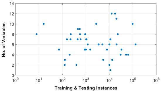
Figure 12.
Number of variables and the size of dataset used to develop each model.
Another ambiguous matter is the appropriate number of input parameters needed for each case. It is not clear if increasing the input features would yield better performance. It was seen that some models used as few as one or two inputs, relying on historical trends for their predictive ability, while others used as many as 12 parameters trying to mimic physical models to map the relations between the input features and the outcome resulting in a high dimensionality and complex models. Still, this could also result in overfitting [32,44]. This is especially true when the data are not enough to account for all input combinations, resulting in a spurious fitting and a decreased predictive skill [111], in which case, researchers resort to some techniques to reduce overfitting, such as stopping training once validation gets worse, introducing weight penalties in the model, or using dimensionality reduction tools such as PCA.
5. Challenges of Using Machine Learning in Coastal Engineering
The challenge of limited training datasets in coastal engineering is multifaceted. While certain coastal areas are actively monitored and possess substantial historical data, these datasets might not cover the diversity of conditions found across all coastal zones globally. For example, sandy coastlines comprise only about a third of the global ice-free coasts [112]. The potential challenges of transfer learning of ML models in coastal applications become apparent due to the significant spatial variability and diverse coastal landforms present along global coastlines. ML models trained on data from a specific coastal area may struggle to generalize well to new areas with different characteristics. Therefore, when applying a pre-trained model to a new coastal zone, it is crucial to evaluate whether the environmental features of that area align with the training data. This consideration underscores the importance of ensuring the representativeness of the training dataset by incorporating diverse data that capture the variability inherent in various coastal environments. Without sufficient diversity in the training data, the performance of the ML model may be limited when applied to new and unseen coastal zones, potentially leading to inaccurate predictions or suboptimal outcomes. Thus, addressing these challenges requires careful attention to dataset curation and model evaluation to ensure the robustness and generalizability of ML-based solutions in coastal applications.
Consequently, to train ML models effectively, scientists and engineers often need to resort to alternative methods, such as using existing numerical models or experimental setups to generate synthetic training data as seen in the previous section. However, the effectiveness of the ML models hinges on the quality and representativeness of the data. If the training data is incomplete or skewed, it will lead to suboptimal performance. This necessitates a careful prior processing of the data and constant validation against real-world observations. The recent surge in remote sensing and satellite monitoring technologies can substantially alleviate this challenge [1]. The volume of data generated by these technologies, characterized by large spatial and temporal scales and high resolution, opens up new possibilities for leveraging multidimensional and nonlinear datasets for machine learning applications. The challenge now shifts to extracting meaningful insights from this vast and complex data landscape. To aid in this challenge, data filtration, normalization, and database unification become imperative. Shahri et al. [113] present an automated method for processing large datasets and unifying databases.
Additionally, the challenge lies not only in the quantity and quality of the data but also in the selection of input variables. The challenge of selecting suitable input parameters for ML models in coastal engineering is essential for achieving accurate predictions. This requires a clear understanding of the underlying system dynamics. Identifying the key parameters that capture the complexities of the studied coastal engineering case is an iterative process and involves domain expertise to recognize the relevant features influencing the system.
The question of which ML technique to use for a specific task also introduces complexity. Coastal processes are highly dynamic and involve complex interactions. Selecting the most suitable ML algorithm is a critical decision in the modeling process. The challenge is to match the characteristics of the coastal engineering problem with the strengths and weaknesses of different algorithms. Different tasks, such as storm surge prediction or sediment transport modeling, may benefit from distinct ML methodologies. Predicting beach erosion might require a different ML approach than predicting wave patterns, for instance. This decision is influenced by factors such as the nature of the data, the complexity of the problem, and the desired outcomes. The challenge is to navigate this landscape effectively, experimenting with different algorithms and iteratively refining the approach to find the one that provides the most efficient and accurate representation of the specific problem at hand. It is nearly impossible to know which ML technique is best suited for a given problem, except through trial and error or inferring from others’ work. Even then, different data structures or a desired outcome of the same problem could benefit from different methods. Techniques such as Bayesian networks, Gaussian-based models, and ANNs can be first explored if the user is looking for a probabilistic answer for a problem. If the problem is classification based, then decision trees and SVMs can be employed. For problems that depend on multiple parameters and smooth or continuous outputs, ANNs, genetic programming, and ANFISs can be used.
These challenges and knowledge gaps require further examination by future research. Conducting benchmarking studies and comparative analysis on different ML models can help elucidate these topics. Goldstein et al. [41] advocate making coastal ML research more transferable and reproducible. They present some practices for researchers to follow which would help reach this goal, some of which include making datasets available, providing the weights of the model, mentioning the data-splitting technique, and defining the metrics for model testing. These practices allow others to reproduce, compare, and critique different models, eventually resulting in the buildup of knowledge.
6. Conclusions
The application of machine learning in coastal engineering presents a transformative potential for how coastal processes are understood and modeled. Traditional empirical and numerical models have served as the backbone for simulating coastal processes, offering a blend of precision and effectiveness. However, the increasing complexity and computational demands of these models have catalyzed a shift towards data-driven techniques that have the potential to substitute traditional techniques in the future. The review highlights the growing preference for ML techniques in coastal engineering applications, especially in the areas of wave pattern prediction, water level fluctuation, and morphology change. This is by no means an exhaustive list of all the articles published in this regard, nor all available ML algorithms. This article intends to showcase the recent advancements made in the field and the capacity of different ML techniques to leverage vast amounts of data to simulate complex coastal phenomena with greater efficiency and reduced computational costs. Also, there is no doubt that as newer algorithms emerge, they will continue to be applied in coastal research, which might overthrow all the challenges currently experienced.
ML models have not only demonstrated improved prediction skills over traditional methods but have also offered substantial computational advantages, facilitating real-time decision-making. Despite the promise of ML, challenges remain, particularly concerning the availability and quality of training data, the interpretability of ML models, the selection of suitable algorithms and features, and the generalization of the developed models. Moreover, as ML techniques are intrinsically data-driven, their success is contingent upon the availability of high-quality and representative datasets to train the models, which can be a limiting factor in most cases. To harness the full potential of ML in coastal engineering, future research must focus on enhancing the robustness, accuracy, and applicability of these models. This includes addressing questions about the quantity and quality of the data, understanding which methods work best for which problems, and improving methodologies for model training and validation. The emergence of automated machine learning (AutoML) can help address questions related to the applicability and optimization of ML algorithms. AutoML promises to automate the ML development process to include processes such as data preparation, input selection, model generation, and evaluation [114]. As stated by [115], AutoML aims to enable domain scientists to build ML applications without extensive knowledge in statistics or machine learning, thus reducing the demand for data scientists. This will undoubtedly increase the adoption of ML in coastal engineering and help discover other techniques from the data sciences. The reviewed literature points to an exciting future where ML not only complements but, in many cases, significantly enhances our capabilities to predict and manage the complex dynamics of coastal environments.
Author Contributions
Conceptualization, M.A., P.R.-S., L.d.N. and F.T.-P.; methodology, M.A., P.R.-S., L.d.N. and F.T.-P.; formal analysis, M.A.; investigation, M.A.; resources, P.R.-S., L.d.N. and F.T.-P.; data curation, M.A.; writing—original draft preparation, M.A.; writing—review and editing, M.A., P.R.-S., L.d.N. and F.T.-P.; visualization, M.A., P.R.-S., L.d.N. and F.T.-P.; supervision, P.R.-S., L.d.N. and F.T.-P.; project administration, P.R.-S., L.d.N. and F.T.-P. funding acquisition, M.A., P.R.-S., L.d.N. and F.T.-P. All authors have read and agreed to the published version of the manuscript.
Funding
Part of this research has received funding from the European Union’s Horizon Europe research and innovation programme under grant agreement No. 101135410—The DuneFront Project.
Acknowledgments
The authors would like to thank the University of Porto as the hosting institution.
Conflicts of Interest
The authors declare no conflicts of interest.
References
- Vitousek, S.; Buscombe, D.; Vos, K.; Barnard, P.L.; Ritchie, A.C.; Warrick, J.A. The future of coastal monitoring through satellite remote sensing. Camb. Prism. Coast. Futur. 2022, 1, e10. [Google Scholar] [CrossRef]
- van Rijn, L.C. Unified View of Sediment Transport by Currents and Waves. I: Initiation of Motion, Bed Roughness, and Bed-Load Transport. J. Hydraul. Eng. 2007, 133, 649–667. [Google Scholar] [CrossRef]
- Holthuijsen, L.H. Waves in Oceanic and Coastal Waters; Cambridge University Press (CUP): Cambridge, UK, 2007. [Google Scholar]
- Dietrich, J.C.; Tanaka, S.; Westerink, J.J.; Dawson, C.N.; Luettich, R.A., Jr.; Zijlema, M.; Holthuijsen, L.H.; Smith, J.M.; Westerink, L.G.; Westerink, H.J. Performance of the Unstructured-Mesh, SWAN+ADCIRC Model in Computing Hurricane Waves and Surge. J. Sci. Comput. 2012, 52, 468–497. [Google Scholar] [CrossRef]
- Nelson, T.R.; Voulgaris, G.; Traykovski, P. Predicting wave-induced ripple equilibrium geometry. J. Geophys. Res. Oceans 2013, 118, 3202–3220. [Google Scholar] [CrossRef]
- Roelvink, D.; Reniers, A.; Van Dongeren, A.P.; De Vries, J.V.T.; McCall, R.; Lescinski, J. Modelling storm impacts on beaches, dunes and barrier islands. Coast. Eng. 2009, 56, 1133–1152. [Google Scholar] [CrossRef]
- Jan, C.-D.; Tseng, C.-M.; Wang, J.-S.; Cheng, Y.-H. Empirical relation between the typhoon surge deviation and the corresponding typhoon characteristics: A case study in Taiwan. J. Mar. Sci. Technol. 2006, 11, 193–200. [Google Scholar] [CrossRef]
- Stockdon, H.F.; Holman, R.A.; Howd, P.A.; Sallenger, A.H., Jr. Empirical parameterization of setup, swash, and runup. Coast. Eng. 2006, 53, 573–588. [Google Scholar] [CrossRef]
- Simmons, J.A.; Splinter, K.D. A multi-model ensemble approach to coastal storm erosion prediction. Environ. Model. Softw. 2022, 150, 105356. [Google Scholar] [CrossRef]
- Sanchez, A.; Wu, W.; Beck, T.M. A depth-averaged 2-D model of flow and sediment transport in coastal waters. Ocean Dyn. 2016, 66, 1475–1495. [Google Scholar] [CrossRef]
- Dey, S.; Ali, S.Z.; Padhi, E. Advances in analytical modeling of suspended sediment transport. J. Hydro-Environ. Res. 2018, 20, 110–126. [Google Scholar] [CrossRef]
- Vyzikas, T. Application of numerical models and codes. Task 3.4.4 of WP3 from the MERiFIC Project. 2014. Available online: https://archimer.ifremer.fr/doc/00324/43550/ (accessed on 10 November 2023).
- Reeve, D.E.; Karunarathna, H.; Pan, S.; Horrillo-Caraballo, J.M.; Różyński, G.; Ranasinghe, R. Data-driven and hybrid coastal morphological prediction methods for mesoscale forecasting. Geomorphology 2016, 256, 49–67. [Google Scholar] [CrossRef]
- LeCun, Y.; Bengio, Y.; Hinton, G. Deep learning. Nature 2015, 521, 436–444. [Google Scholar] [CrossRef]
- Wei, Z.; Davison, A. A convolutional neural network based model to predict nearshore waves and hydrodynamics. Coast. Eng. 2022, 171, 104044. [Google Scholar] [CrossRef]
- James, S.C.; Zhang, Y.; O’Donncha, F. A machine learning framework to forecast wave conditions. Coast. Eng. 2018, 137, 1–10. [Google Scholar] [CrossRef]
- Murphy, K.P. Machine Learning: A Probabilistic Perspective; MIT Press: Cambridge, MA, USA, 2012. [Google Scholar]
- Bonaccorso, G. Machine Learning Algorithms; Packt Publishing Ltd.: Birmingham, UK, 2017. [Google Scholar]
- Beuzen, T.; Splinter, K. Machine learning and coastal processes. In Sandy Beach Morphodynamics; Elsevier: Amsterdam, The Netherlands, 2020; pp. 689–710. [Google Scholar] [CrossRef]
- Liu, C.M.; Rim, D.; Baraldi, R.; LeVeque, R.J. Comparison of Machine Learning Approaches for Tsunami Forecasting from Sparse Observations. Pure Appl. Geophys. 2021, 178, 5129–5153. [Google Scholar] [CrossRef]
- Mulia, I.E.; Gusman, A.R.; Satake, K. Applying a Deep Learning Algorithm to Tsunami Inundation Database of Megathrust Earthquakes. J. Geophys. Res. Solid Earth 2020, 125, e2020JB019690. [Google Scholar] [CrossRef]
- Wang, Y.; Imai, K.; Miyashita, T.; Ariyoshi, K.; Takahashi, N.; Satake, K. Coastal tsunami prediction in Tohoku region, Japan, based on S-net observations using artificial neural network. Earth Planets Space 2023, 75, 154. [Google Scholar] [CrossRef]
- Etemad-Shahidi, A.; Yasa, R.; Kazeminezhad, M. Prediction of wave-induced scour depth under submarine pipelines using machine learning approach. Appl. Ocean Res. 2011, 33, 54–59. [Google Scholar] [CrossRef]
- Kumar, L.; Afzal, M.S. Estimating pier scour depth under combined waves and current using boosting machine-learning models. Acta Geophys. 2023, 1–17. [Google Scholar] [CrossRef]
- Pourzangbar, A.; Brocchini, M.; Saber, A.; Mahjoobi, J.; Mirzaaghasi, M.; Barzegar, M. Prediction of scour depth at breakwaters due to non-breaking waves using machine learning approaches. Appl. Ocean Res. 2017, 63, 120–128. [Google Scholar] [CrossRef]
- Kim, T.; Kwon, S.; Kwon, Y. Prediction of wave transmission characteristics of low-crested structures with comprehensive analysis of machine learning. Sensors 2021, 21, 8192. [Google Scholar] [CrossRef] [PubMed]
- Gandomi, M.; Pirooz, M.D.; Varjavand, I.; Nikoo, M.R. Permeable breakwaters performance modeling: A comparative study of machine learning techniques. Remote Sens. 2020, 12, 1856. [Google Scholar] [CrossRef]
- Saha, S.; Changdar, S.; De, S. Prediction of the stability number of conventional rubble-mound breakwaters using machine learning algorithms. J. Ocean Eng. Sci. 2022. [Google Scholar] [CrossRef]
- Juan, N.P.; Valdecantos, V.N. Review of the application of Artificial Neural Networks in ocean engineering. Ocean Eng. 2022, 259, 111947. [Google Scholar] [CrossRef]
- Hastie, T.; Tibshirani, R.; Friedman, J.H.; Friedman, J.H. The Elements of Statistical Learning: Data Mining, Inference, and Prediction; Springer: New York, NY, USA, 2009; Volume 2. [Google Scholar]
- Ellenson, A.; Pei, Y.; Wilson, G.; Özkan-Haller, H.T.; Fern, X. An application of a machine learning algorithm to determine and describe error patterns within wave model output. Coast. Eng. 2020, 157, 103595. [Google Scholar] [CrossRef]
- Demetriou, D.; Michailides, C.; Papanastasiou, G.; Onoufriou, T. Nowcasting significant wave height prediction by supervised machine learning classification algorithms. Ocean Eng. 2021, 242, 110130. [Google Scholar] [CrossRef]
- Guillou, N.; Chapalain, G. Machine learning methods applied to sea level predictions in the upper part of a tidal estuary. Oceanologia 2021, 63, 531–544. [Google Scholar] [CrossRef]
- Elith, J.; Leathwick, J.R.; Hastie, T. A working guide to boosted regression trees. J. Anim. Ecol. 2008, 77, 802–813. [Google Scholar] [CrossRef]
- Beuzen, T.; Marshall, L.; Splinter, K.D. A comparison of methods for discretizing continuous variables in Bayesian Networks. Environ. Model. Softw. 2018, 108, 61–66. [Google Scholar] [CrossRef]
- Chen, S.H.; Pollino, C.A. Good practice in Bayesian network modelling. Environ. Model. Softw. 2012, 37, 134–145. [Google Scholar] [CrossRef]
- Uusitalo, L. Advantages and challenges of Bayesian networks in environmental modelling. Ecol. Model. 2007, 203, 312–318. [Google Scholar] [CrossRef]
- Smola, A.J.; Schölkopf, B. A tutorial on support vector regression. Stat. Comput. 2004, 14, 199–222. [Google Scholar] [CrossRef]
- Malekmohamadi, I.; Bazargan-Lari, M.R.; Kerachian, R.; Nikoo, M.R.; Fallahnia, M. Evaluating the efficacy of SVMs, BNs, ANNs and ANFIS in wave height prediction. Ocean Eng. 2011, 38, 487–497. [Google Scholar] [CrossRef]
- Makarynskyy, O. Improving wave predictions with artificial neural networks. Ocean Eng. 2004, 31, 709–724. [Google Scholar] [CrossRef]
- Goldstein, E.B.; Coco, G.; Plant, N.G. A review of machine learning applications to coastal sediment transport and morphodynamics. Earth-Sci. Rev. 2019, 194, 97–108. [Google Scholar] [CrossRef]
- Fan, S.; Xiao, N.; Dong, S. A novel model to predict significant wave height based on long short-term memory network. Ocean Eng. 2020, 205, 107298. [Google Scholar] [CrossRef]
- Gracia, S.; Olivito, J.; Resano, J.; Martin-Del-Brio, B.; de Alfonso, M.; Álvarez, E. Improving accuracy on wave height estimation through machine learning techniques. Ocean Eng. 2021, 236, 108699. [Google Scholar] [CrossRef]
- Srivastava, N.; Hinton, G.; Krizhevsky, A.; Sutskever, I.; Salakhutdinov, R. Dropout: A simple way to prevent neural networks from overfitting. J. Mach. Learn. Res. 2014, 15, 1929–1958. [Google Scholar]
- Deo, M.; Jha, A.; Chaphekar, A.; Ravikant, K. Neural networks for wave forecasting. Ocean Eng. 2001, 28, 889–898. [Google Scholar] [CrossRef]
- Mahjoobi, J.; Etemad-Shahidi, A. An alternative approach for the prediction of significant wave heights based on classification and regression trees. Appl. Ocean Res. 2008, 30, 172–177. [Google Scholar] [CrossRef]
- Günaydın, K. The estimation of monthly mean significant wave heights by using artificial neural network and regression methods. Ocean Eng. 2008, 35, 1406–1415. [Google Scholar] [CrossRef]
- Mahjoobi, J.; Etemad-Shahidi, A.; Kazeminezhad, M. Hindcasting of wave parameters using different soft computing methods. Appl. Ocean Res. 2008, 30, 28–36. [Google Scholar] [CrossRef]
- Berbić, J.; Ocvirk, E.; Carević, D.; Lončar, G. Application of neural networks and support vector machine for significant wave height prediction. Oceanologia 2017, 59, 331–349. [Google Scholar] [CrossRef]
- Kumar, N.K.; Savitha, R.; Al Mamun, A. Regional ocean wave height prediction using sequential learning neural networks. Ocean Eng. 2017, 129, 605–612. [Google Scholar] [CrossRef]
- Mahmoodi, K.; Nowruzi, H. Extreme wave height detection based on the meteorological data, using hybrid NOF-ELM method. Ships Offshore Struct. 2022, 17, 2520–2530. [Google Scholar] [CrossRef]
- Wei, Z. Forecasting wind waves in the US Atlantic Coast using an artificial neural network model: Towards an AI-based storm forecast system. Ocean Eng. 2021, 237, 109646. [Google Scholar] [CrossRef]
- Jörges, C.; Berkenbrink, C.; Stumpe, B. Prediction and reconstruction of ocean wave heights based on bathymetric data using LSTM neural networks. Ocean Eng. 2021, 232, 109046. [Google Scholar] [CrossRef]
- Liu, T.; Zhang, Y.; Qi, L.; Dong, J.; Lv, M.; Wen, Q. WaveNet: Learning to predict wave height and period from accelerometer data using convolutional neural network. IOP Conf. Ser. Earth Environ. Sci. 2019, 369, 012001. [Google Scholar] [CrossRef]
- Ma, X.; Huang, L.; Duan, W.; Jing, Y.; Zheng, Q. The performance and optimization of ANN-WP model under unknown sea states. Ocean Eng. 2021, 239, 109858. [Google Scholar] [CrossRef]
- Duan, W.; Ma, X.; Huang, L.; Liu, Y.; Duan, S. Phase-resolved wave prediction model for long-crest waves based on machine learning. Comput. Methods Appl. Mech. Eng. 2020, 372, 113350. [Google Scholar] [CrossRef]
- Malekmohamadi, I.; Ghiassi, R.; Yazdanpanah, M. Wave hindcasting by coupling numerical model and artificial neural networks. Ocean Eng. 2008, 35, 417–425. [Google Scholar] [CrossRef]
- O’donncha, F.; Zhang, Y.; Chen, B.; James, S.C. Ensemble model aggregation using a computationally lightweight machine-learning model to forecast ocean waves. J. Mar. Syst. 2019, 199, 103206. [Google Scholar] [CrossRef]
- Wang, N.; Chen, Q.; Chen, Z. Reconstruction of nearshore wave fields based on physics-informed neural networks. Coast. Eng. 2022, 176, 104167. [Google Scholar] [CrossRef]
- Chang, H.-K.; Liou, J.-C.; Liu, S.-J.; Liaw, S.-R. Simulated wave-driven ANN model for typhoon waves. Adv. Eng. Softw. 2011, 42, 25–34. [Google Scholar] [CrossRef]
- O’donncha, F.; Zhang, Y.; Chen, B.; James, S.C. An integrated framework that combines machine learning and numerical models to improve wave-condition forecasts. J. Mar. Syst. 2018, 186, 29–36. [Google Scholar] [CrossRef]
- Makarynskyy, O. Neural pattern recognition and prediction for wind wave data assimilation. Pac. Oceanogr. 2005, 3, 76–85. [Google Scholar]
- Londhe, S.N.; Shah, S.; Dixit, P.R.; Nair, T.M.B.; Sirisha, P.; Jain, R. A Coupled Numerical and Artificial Neural Network Model for Improving Location Specific Wave Forecast. Appl. Ocean Res. 2016, 59, 483–491. [Google Scholar] [CrossRef]
- Sztobryn, M. Forecast of storm surge by means of artificial neural network. J. Sea Res. 2003, 49, 317–322. [Google Scholar] [CrossRef]
- Lee, T.-L. Neural network prediction of a storm surge. Ocean Eng. 2006, 33, 483–494. [Google Scholar] [CrossRef]
- Lee, T.-L. Back-propagation neural network for the prediction of the short-term storm surge in Taichung harbor, Taiwan. Eng. Appl. Artif. Intell. 2008, 21, 63–72. [Google Scholar] [CrossRef]
- Tseng, C.; Jan, C.; Wang, J.; Wang, C. Application of artificial neural networks in typhoon surge forecasting. Ocean Eng. 2007, 34, 1757–1768. [Google Scholar] [CrossRef]
- Rajasekaran, S.; Gayathri, S.; Lee, T.-L. Support vector regression methodology for storm surge predictions. Ocean Eng. 2008, 35, 1578–1587. [Google Scholar] [CrossRef]
- Hashemi, M.R.; Spaulding, M.L.; Shaw, A.; Farhadi, H.; Lewis, M. An efficient artificial intelligence model for prediction of tropical storm surge. Nat. Hazards 2016, 82, 471–491. [Google Scholar] [CrossRef]
- Jia, G.; Taflanidis, A.A. Kriging metamodeling for approximation of high-dimensional wave and surge responses in real-time storm/hurricane risk assessment. Comput. Methods Appl. Mech. Eng. 2013, 261–262, 24–38. [Google Scholar] [CrossRef]
- Taflanidis, A.A.; Jia, G.; Kennedy, A.B.; Smith, J.M. Implementation/optimization of moving least squares response surfaces for approximation of hurricane/storm surge and wave responses. Nat. Hazards 2013, 66, 955–983. [Google Scholar] [CrossRef]
- Kim, S.-W.; Melby, J.A.; Nadal-Caraballo, N.C.; Ratcliff, J. A time-dependent surrogate model for storm surge prediction based on an artificial neural network using high-fidelity synthetic hurricane modeling. Nat. Hazards 2015, 76, 565–585. [Google Scholar] [CrossRef]
- Jia, G.; Taflanidis, A.A.; Nadal-Caraballo, N.C.; Melby, J.A.; Kennedy, A.B.; Smith, J.M. Surrogate modeling for peak or time-dependent storm surge prediction over an extended coastal region using an existing database of synthetic storms. Nat. Hazards 2016, 81, 909–938. [Google Scholar] [CrossRef]
- Lee, J.-W.; Irish, J.L.; Bensi, M.T.; Marcy, D.C. Rapid prediction of peak storm surge from tropical cyclone track time series using machine learning. Coast. Eng. 2021, 170, 104024. [Google Scholar] [CrossRef]
- Bass, B.; Bedient, P. Surrogate modeling of joint flood risk across coastal watersheds. J. Hydrol. 2018, 558, 159–173. [Google Scholar] [CrossRef]
- Al Kajbaf, A.; Bensi, M. Application of surrogate models in estimation of storm surge:A comparative assessment. Appl. Soft Comput. 2020, 91, 106184. [Google Scholar] [CrossRef]
- Riazi, A. Accurate tide level estimation: A deep learning approach. Ocean Eng. 2020, 198, 107013. [Google Scholar] [CrossRef]
- Ishida, K.; Tsujimoto, G.; Ercan, A.; Tu, T.; Kiyama, M.; Amagasaki, M. Hourly-scale coastal sea level modeling in a changing climate using long short-term memory neural network. Sci. Total Environ. 2020, 720, 137613. [Google Scholar] [CrossRef]
- Accarino, G.; Chiarelli, M.; Fiore, S.; Federico, I.; Causio, S.; Coppini, G.; Aloisio, G. A multi-model architecture based on Long Short-Term Memory neural networks for multi-step sea level forecasting. Future Gener. Comput. Syst. 2021, 124, 1–9. [Google Scholar] [CrossRef]
- Zhang, J.; Taflanidis, A.A.; Nadal-Caraballo, N.C.; Melby, J.A.; Diop, F. Advances in surrogate modeling for storm surge prediction: Storm selection and addressing characteristics related to climate change. Nat. Hazards 2018, 94, 1225–1253. [Google Scholar] [CrossRef]
- Kim, S.; Pan, S.; Mase, H. Artificial neural network-based storm surge forecast model: Practical application to Sakai Minato, Japan. Appl. Ocean Res. 2019, 91, 101871. [Google Scholar] [CrossRef]
- Kyprioti, A.P.; Taflanidis, A.A.; Plumlee, M.; Asher, T.G.; Spiller, E.; Luettich, R.A.; Blanton, B.; Kijewski-Correa, T.L.; Kennedy, A.; Schmied, L. Improvements in storm surge surrogate modeling for synthetic storm parameterization, node condition classification and implementation to small size databases. Nat. Hazards 2021, 109, 1349–1386. [Google Scholar] [CrossRef]
- Shafaghat, M.; Dezvareh, R. Support vector machine for classification and regression of coastal sediment transport. Arab. J. Geosci. 2021, 14, 2009. [Google Scholar] [CrossRef]
- Kamphuis, J.W. Introduction to Coastal Engineering and Management; World Scientific: Singapore, 2020; Volume 48. [Google Scholar]
- Kamphuis, J.W.; Kamphuis, M.J.W.; Member, A. Alongshore sediment transport rate. J. Waterw. Port Coast. Ocean Eng. 1991, 117, 624–640. [Google Scholar] [CrossRef]
- Karaca, Y.; Cattani, C.; Moonis, M. Comparison of Deep Learning and Support Vector Machine Learning for Subgroups of Multiple Sclerosis. In Computational Science and Its Applications—ICCSA 2017; Gervasi, O., Murgante, B., Misra, S., Borruso, G., Torre, C.M., Rocha, A.M.A.C., Taniar, D., Apduhan, B.O., Stankova, E., Cuzzocrea, A., Eds.; Springer International Publishing: Cham, Switzerland, 2017; pp. 142–153. [Google Scholar]
- Dezvareh, R.; Shafaghat, M. Predicting the sediment rate of Nakhilo Port using artificial intelligence. Int. J. Coast. Offshore Environ. Eng. 2020, 5, 41–49. [Google Scholar]
- Phillip, R.; Penko, A.; Palmsten, M.; DuVal, C. A machine learning approach to predicting equilibrium ripple wavelength. Environ. Model. Softw. 2022, 157, 105509. [Google Scholar] [CrossRef]
- Wolpert, D.H. Stacked generalization. Neural Netw. 1992, 5, 241–259. [Google Scholar] [CrossRef]
- Traykovski, P.; Hay, A.E.; Irish, J.D.; Lynch, J.F. Geometry, migration, and evolution of wave orbital ripples at LEO-15. J. Geophys. Res. Oceans 1999, 104, 1505–1524. [Google Scholar] [CrossRef]
- Goldstein, E.B.; Coco, G.; Murray, A.B. Prediction of wave ripple characteristics using genetic programming. Cont. Shelf Res. 2013, 71, 1–15. [Google Scholar] [CrossRef]
- Makarynskyy, O.; Makarynska, D.; Rayson, M.; Langtry, S. Combining deterministic modelling with artificial neural networks for suspended sediment estimates. Appl. Soft Comput. 2015, 35, 247–256. [Google Scholar] [CrossRef]
- Zhang, S.; Wu, J.; Jia, Y.; Wang, Y.-G.; Zhang, Y.; Duan, Q. A temporal LASSO regression model for the emergency forecasting of the suspended sediment concentrations in coastal oceans: Accuracy and interpretability. Eng. Appl. Artif. Intell. 2021, 100, 104206. [Google Scholar] [CrossRef]
- Stachurska, B.; Mahdavi-Meymand, A.; Sulisz, W. Machine learning methodology for determination of sediment particle velocities over sandy and rippled bed. Measurement 2022, 197, 111332. [Google Scholar] [CrossRef]
- Bujak, D.; Bogovac, T.; Carević, D.; Ilic, S.; Lončar, G. Application of artificial neural networks to predict beach nourishment volume requirements. J. Mar. Sci. Eng. 2021, 9, 786. [Google Scholar] [CrossRef]
- Kim, H.D.; Aoki, S.-I. Artificial intelligence application on sediment transport. J. Mar. Sci. Eng. 2021, 9, 600. [Google Scholar] [CrossRef]
- Kumar, P.; Leonardi, N. A novel framework for the evaluation of coastal protection schemes through integration of numerical modelling and artificial intelligence into the Sand Engine App. Sci. Rep. 2023, 13, 8610. [Google Scholar] [CrossRef]
- Harley, M.D.; Turner, I.L.; Short, A.D.; Ranasinghe, R. An empirical model of beach response to storms-SE Australia. In Coasts and Ports; Engineers Australia: Wellington, New Zealand, 2009; pp. 600–606. [Google Scholar]
- de Melo, W.W.; Pinho, J.; Iglesias, I. Coastal morphodynamic emulator for early warning short-term forecasts. Environ. Model. Softw. 2023, 165, 105729. [Google Scholar] [CrossRef]
- de Melo, W.W.; Pinho, J.L.S.; Iglesias, I. Emulating the estuarine morphology evolution using a deep convolutional neural network emulator based on hydrodynamic results of a numerical model. J. Hydroinform. 2022, 24, 1254–1268. [Google Scholar] [CrossRef]
- Santos, V.M.; Wahl, T.; Long, J.W.; Passeri, D.L.; Plant, N.G. Combining numerical and statistical models to predict storm-induced dune erosion. J. Geophys. Res. Earth Surf. 2019, 124, 1817–1834. [Google Scholar] [CrossRef]
- Wahl, T.; Plant, N.G.; Long, J.W. Probabilistic assessment of erosion and flooding risk in the northern Gulf of Mexico. J. Geophys. Res. Oceans 2016, 121, 3029–3043. [Google Scholar] [CrossRef]
- Athanasiou, P.; van Dongeren, A.; Giardino, A.; Vousdoukas, M.; Antolinez, J.A.A.; Ranasinghe, R. Estimating dune erosion at the regional scale using a meta-model based on neural networks. Nat. Hazards Earth Syst. Sci. 2022, 22, 3897–3915. [Google Scholar] [CrossRef]
- Itzkin, M.; Moore, L.J.; Ruggiero, P.; Hovenga, P.A.; Hacker, S.D. Combining process-based and data-driven approaches to forecast beach and dune change. Environ. Model. Softw. 2022, 153, 105404. [Google Scholar] [CrossRef]
- Beuzen, T.; Goldstein, E.B.; Splinter, K.D. Ensemble models from machine learning: An example of wave runup and coastal dune erosion. Nat. Hazards Earth Syst. Sci. 2019, 19, 2295–2309. [Google Scholar] [CrossRef]
- Montaño, J.; Coco, G.; Antolínez, J.A.A.; Beuzen, T.; Bryan, K.R.; Cagigal, L.; Castelle, B.; Davidson, M.A.; Goldstein, E.B.; Ibaceta, R.; et al. Blind testing of shoreline evolution models. Sci. Rep. 2020, 10, 2137. [Google Scholar] [CrossRef]
- Clemente, D.; Teixeira-Duarte, F.; Rosa-Santos, P.; Taveira-Pinto, F. Advancements on Optimization Algorithms Applied to Wave Energy Assessment: An Overview on Wave Climate and Energy Resource. Energies 2023, 16, 4660. [Google Scholar] [CrossRef]
- Tu, J.V. Advantages and disadvantages of using artificial neural networks versus logistic regression for predicting medical outcomes. J. Clin. Epidemiol. 1996, 49, 1225–1231. [Google Scholar] [CrossRef]
- Shah, S.A.R.; Brijs, T.; Ahmad, N.; Pirdavani, A.; Shen, Y.; Basheer, M.A. Road safety risk evaluation using gis-based data envelopment analysis—Artificial neural networks approach. Appl. Sci. 2017, 7, 886. [Google Scholar] [CrossRef]
- Hochreiter, S.; Schmidhuber, J. Long short-term memory. Neural Comput. 1997, 9, 1735–1780. [Google Scholar] [CrossRef]
- Beuzen, T.; Splinter, K.D.; Turner, I.L.; Harley, M.D.; Marshall, L. Predicting storm erosion on sandy coastlines using a Bayesian network. In Proceedings of the Australasian Coasts and Ports 2017 Conference, Cairns, Australia, 21–23 June 2017; pp. 21–23. [Google Scholar]
- Luijendijk, A.; Hagenaars, G.; Ranasinghe, R.; Baart, F.; Donchyts, G.; Aarninkhof, S. The state of the world’s beaches. Sci. Rep. 2018, 8, 6641. [Google Scholar] [CrossRef]
- Shahri, A.A.; Shan, C.; Larsson, S.; Johansson, F. Normalizing Large Scale Sensor-Based MWD Data: An Automated Method toward A Unified Database. Sensors 2024, 24, 1209. [Google Scholar] [CrossRef]
- He, X.; Zhao, K.; Chu, X. AutoML: A survey of the state-of-the-art. Knowl.-Based Syst. 2021, 212, 106622. [Google Scholar] [CrossRef]
- Zöller, M.-A.; Huber, M.F. Benchmark and survey of automated machine learning frameworks. J. Artif. Intell. Res. 2021, 70, 409–472. [Google Scholar] [CrossRef]
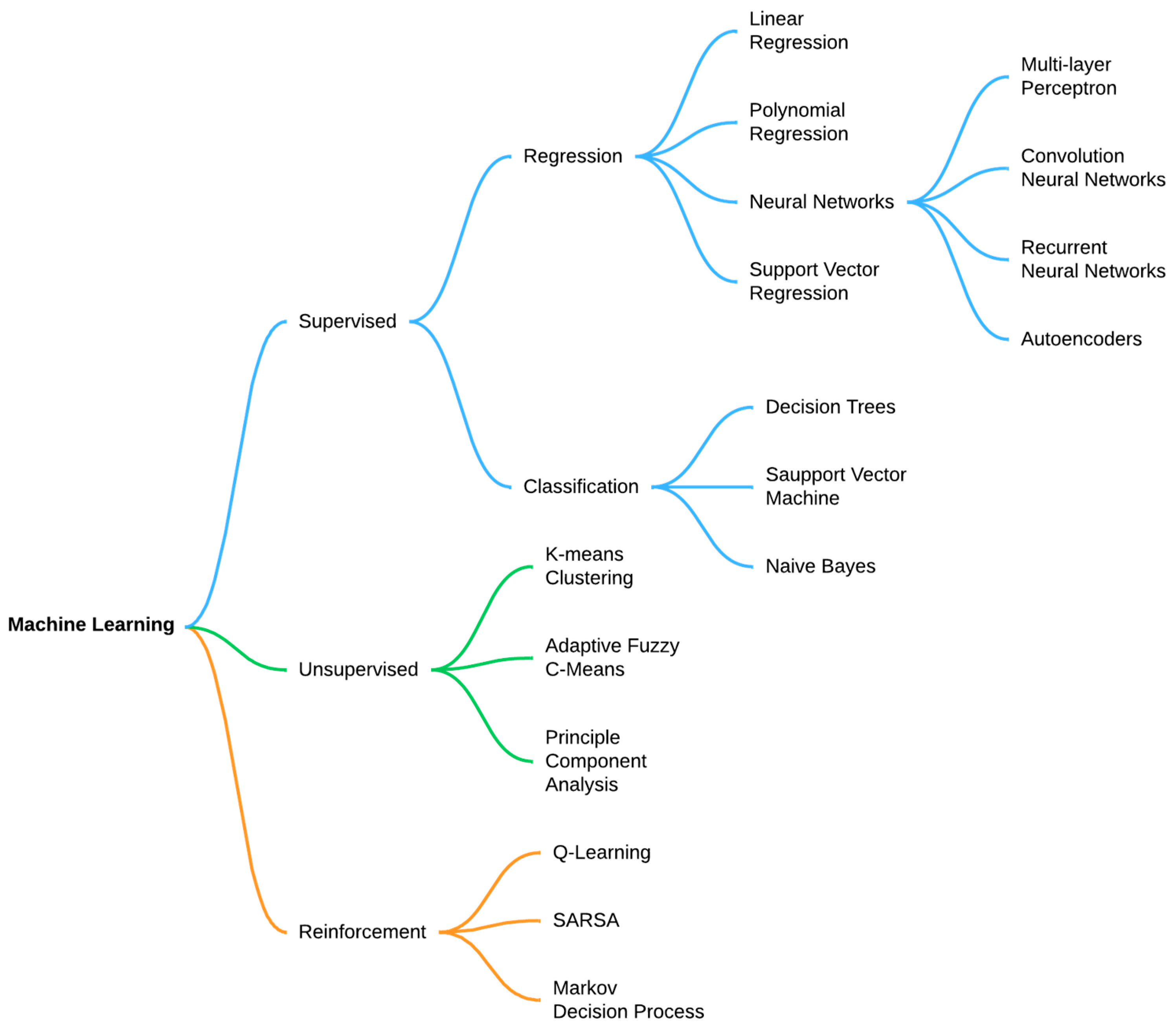
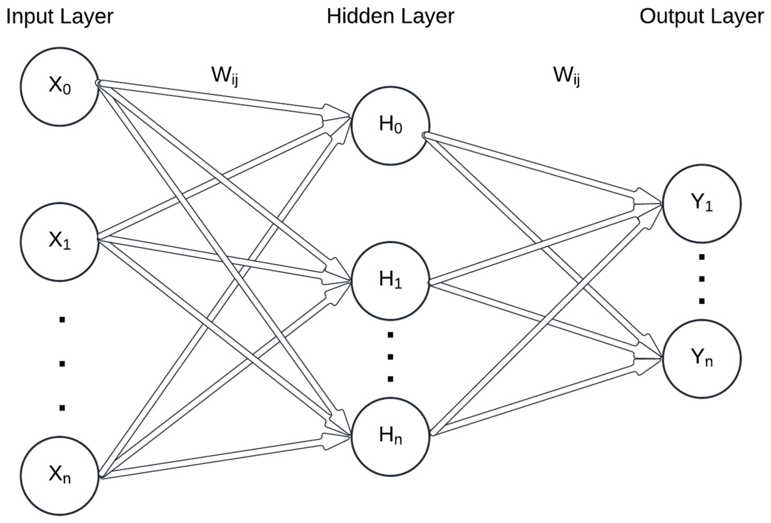

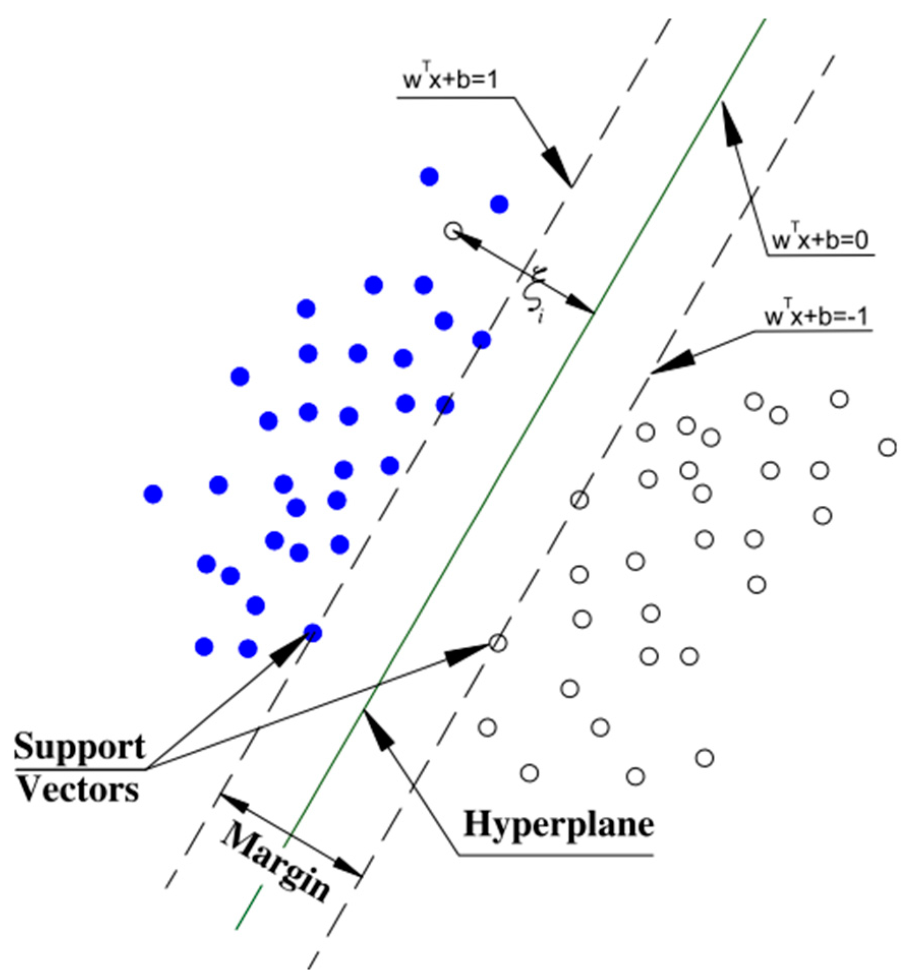
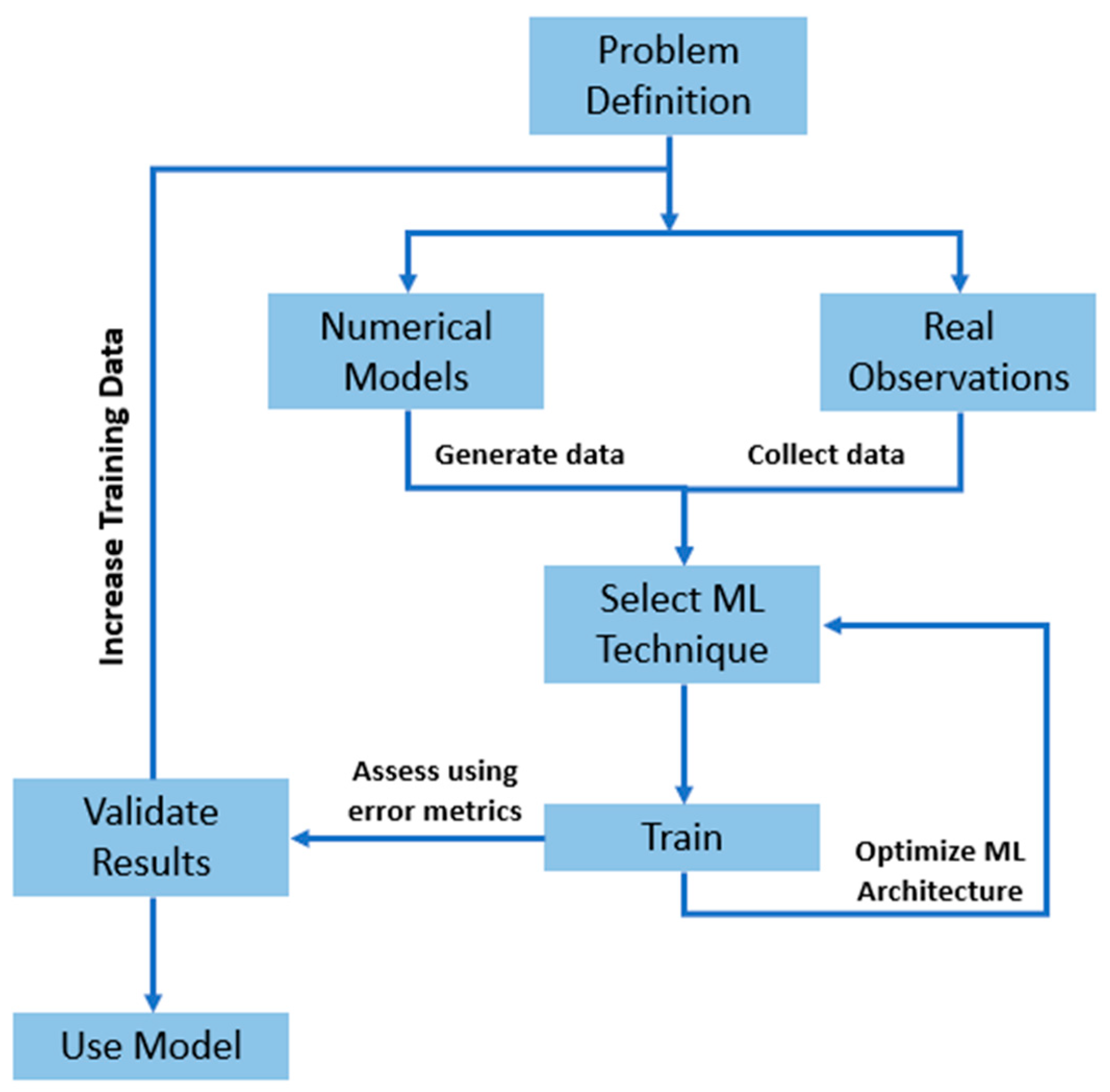
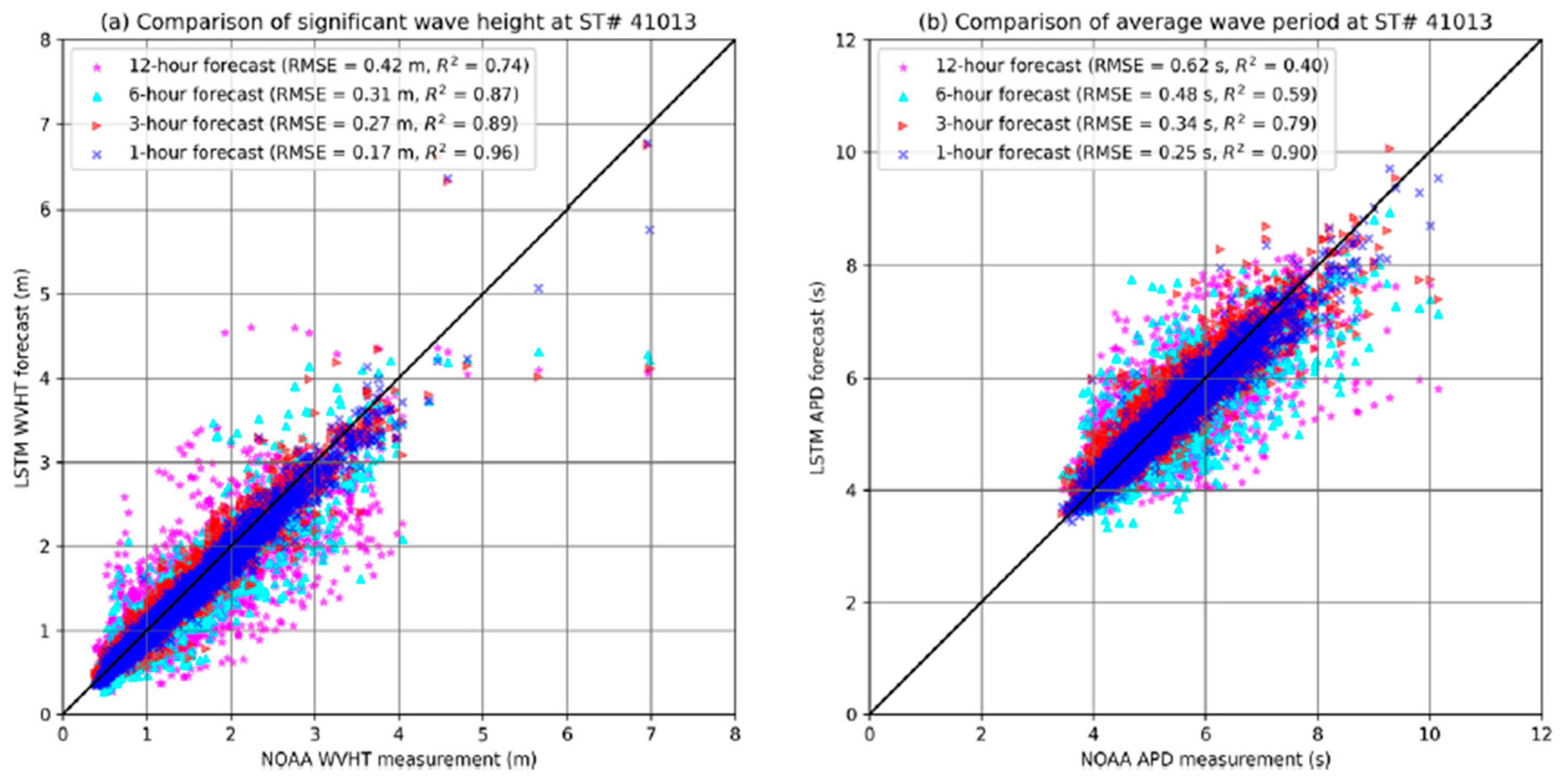

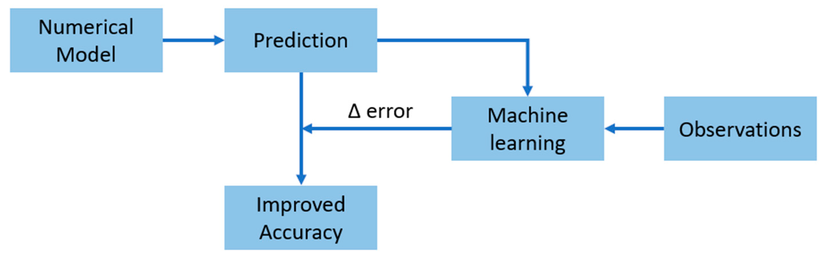

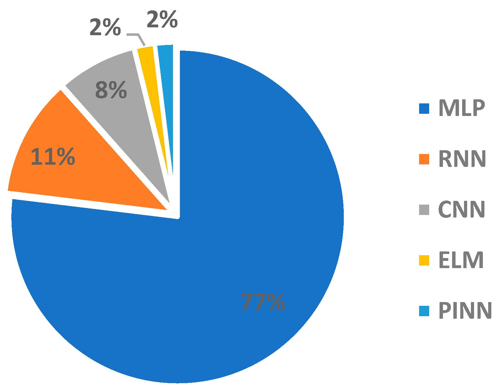
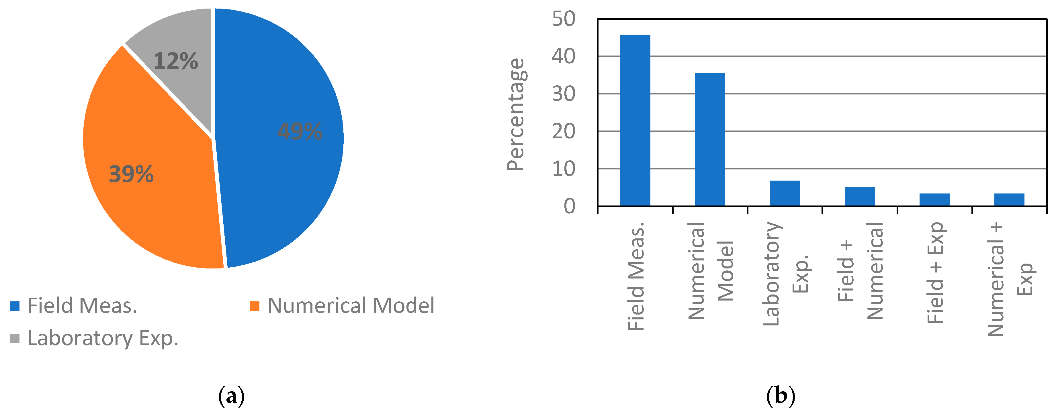
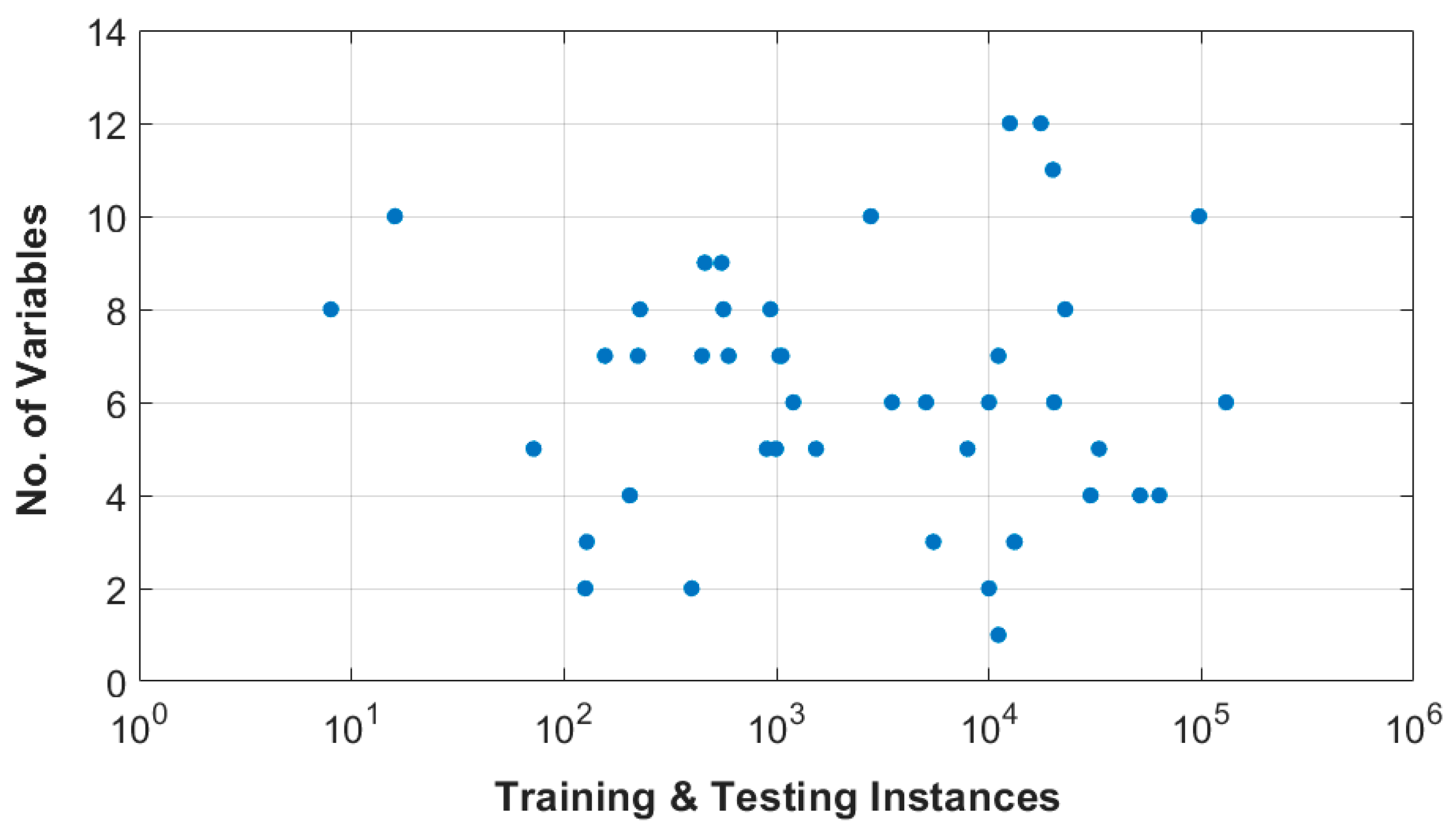
Disclaimer/Publisher’s Note: The statements, opinions and data contained in all publications are solely those of the individual author(s) and contributor(s) and not of MDPI and/or the editor(s). MDPI and/or the editor(s) disclaim responsibility for any injury to people or property resulting from any ideas, methods, instructions or products referred to in the content. |
© 2024 by the authors. Licensee MDPI, Basel, Switzerland. This article is an open access article distributed under the terms and conditions of the Creative Commons Attribution (CC BY) license (https://creativecommons.org/licenses/by/4.0/).