A Comparison of Methods of Visual Census and Cryptobenthic Fish Collecting, an Integrative Approach to the Qualitative and Quantitative Composition of the Mediterranean Temperate Reef Fish Assemblages

Abstract

The present research quantitatively compared the fish composition among two methods for non-cryptic benthic fish species and one method for cryptobenthic fish species for the first time for the Mediterranean temperate reef fish assemblage. A visual census of fishes was performed within a cylinder of 4 m radius and within a cylinder of 2 m radius, while the cryptobenthic fishes were collected using a square of 1 m² with anesthetic. The data and material were collected at fifty sampling points. The visual census methods together recorded 31 species, and the square with anesthetic method recorded 18 species. The quantitative comparison of methods of visual census and cryptobenthic fish collecting showed significantly different species richness, total fish abundance, and fish assemblage structure among methods. The applied methods were highly complementary. The cylinder of 2 m radius is well suited for epibenthic fishes and the cylinder of 4 m radius is reliable for hyperbenthic and benthopelagic fishes. Therefore, each of the methods well covered one of three components of ichthyobenthos (hyperbenthic, epibenthic, and cryptobenthic fishes), and all three methods together provided a far more complete assessment of fish species composition than any individual census method for the Mediterranean littoral benthic fishes.

1. Introduction

Underwater visual census with in-situ observation and recording of data by SCUBA divers is a commonly used method to study reef fish assemblages and is a standard technique for estimation of benthic fish abundance [1]. The method of underwater visual census was introduced in the 1950s [2]. In the Mediterranean, the method has been used since the 1970s [3,4]. However, it has been noticed that visual census misses the presence or underestimates the abundance of cryptic fish species [5]. Visual census methods mostly fail to record cryptobenthic fishes [6,7,8]. The proportion of the biodiversity of the fish assemblage unrecorded in visual census researches, when later checked by application of ichthyocide, was very high [8]. Smith-Vaniz et al. [8] visually recorded only 36% of 228 fish species they sampled by rotenone. Kovačić et al. [9] showed that this cryptobenthic component of the littoral benthic fish assemblage can be successfully collected and quantitatively assessed by the method of anesthetic applied on 1 m² squares. Surprisingly, the examples of combined application of both quantitative methods, visual census and cryptobenthic fish sampling, are quite rare and come mostly from the tropical reefs [5,6,7,8,10]. A few combined studies addressed temperate sea fish assemblages: New Zealand in the South Pacific [7], Portugal in the Northeastern Atlantic [11], as well as Italy [12] and Croatia [13] in the Mediterranean. Mazzoldi and De Girolamo [12] combined a quantitative visual census with a qualitative assessment of the littoral fish assemblage in the Central Mediterranean Sea, at the island of Lampedusa in Italy. The qualitative assessment of the fish assemblage was based on two methods: haphazard visual census surveys, and application of the anesthetic Quinaldine under rocks and inside holes and crevices, recording all observed fish species [12]. With 77 recorded species, the research showed that the best assessment of the richness of species of littoral fish assemblages is based on the combination of the visual census method and the anesthetic method. Soldo et al. [13] combined the results of the two quantitative methods, the visual census and the square saturated with anesthetic, to produce a far more complete assessment of fish species composition on a Mediterranean coralligenous cliff than any of the individual methods. A total of 76 fish species were recorded on a single coralligenous cliff, supporting the opinion that coralligenous cliffs are important Mediterranean biodiversity hotspots. Regrettably, the species compositions of two methods in Soldo et al. [13] were found to be quantitatively incomparable due to differences in positions, surface size, time, and number of samples between methods. As is evident from the literature cited above, the integration, even of the qualitative data, of visual census and anesthetic methods is uncommon for the Mediterranean and there are no examples in the published literature where samples from the visual census and the square saturated with anesthetic methods have been quantitatively compared in the Mediterranean.

Even among the non-cryptic fishes that can be targeted by the visual census, there is a tendency to neglect small species [14]. The research of Minte-Vera et al. [14], testing two widely used visual census protocols, strip transect and stationary cylinder, on various sizes of the studied area, achieved the best results by combining two superimposed cylinders (2 m and 4 m radii), counting small fish (≤10 cm) in the smaller cylinder and larger fish (>10 cm) in the larger cylinder.

The two stationary cylinders also have the advantage of being able to be combined on the same studied point together with the square saturated with anesthetic method, targeting three different components of reef fish assemblages: larger fish, smaller fish, and hidden, usually very small, fish at the same spot. Therefore, the aim of the present work was to: (1) compare the species richness, fish abundance, and fish assemblage structure from two methods for non-cryptic fish species and from one method for cryptobenthic fish species from the Mediterranean temperate reef fish assemblage; and (2) to provide an integrative assessment of the Mediterranean temperate reef fish assemblage composition in studied localities using complementary methods. This underscores the novelty and significance of our study, which provided a comprehensive quantitative comparison of these three methods, shedding light on their respective strengths and limitations in assessing fish assemblages in the Mediterranean region.

2. Materials and Methods

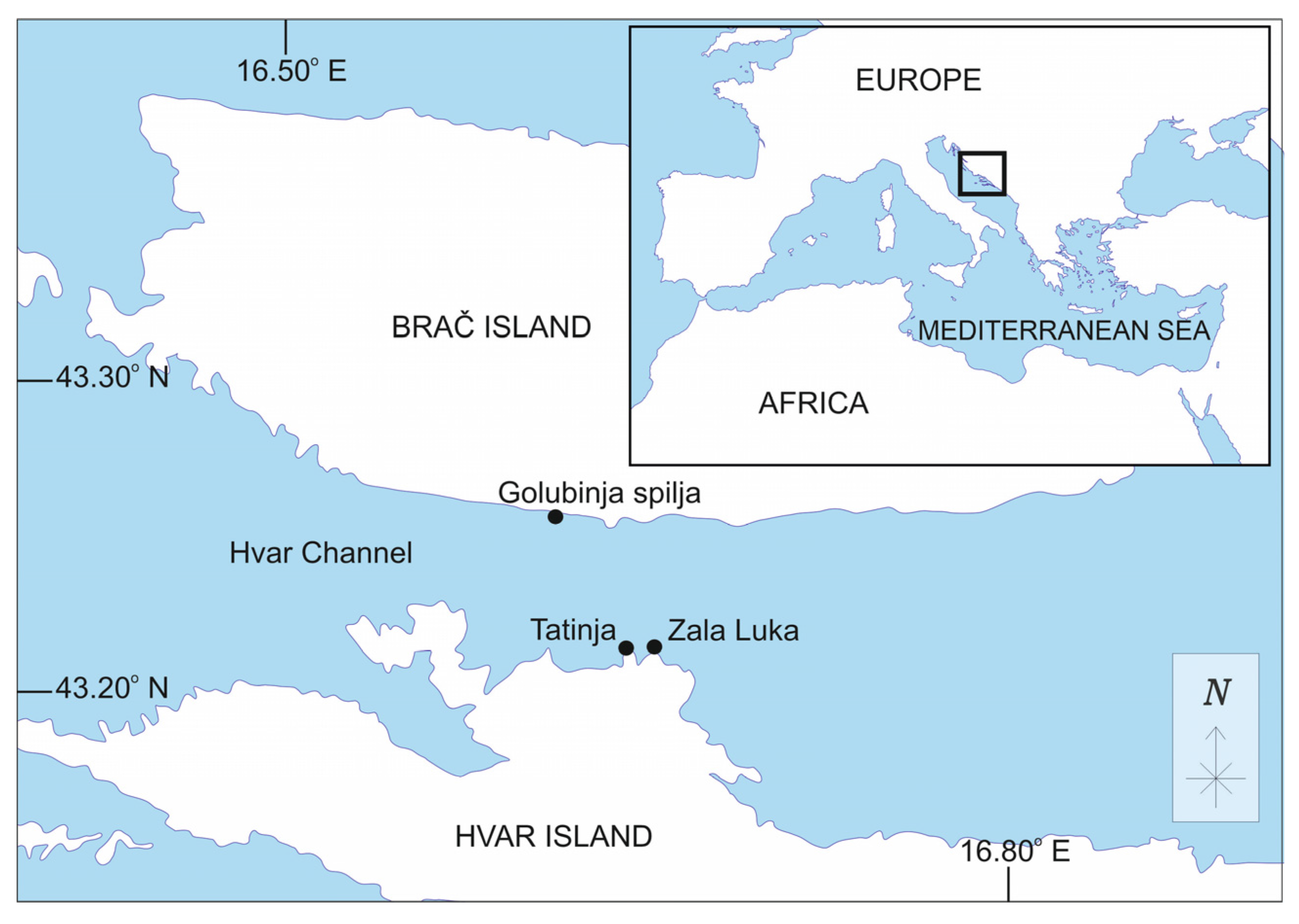
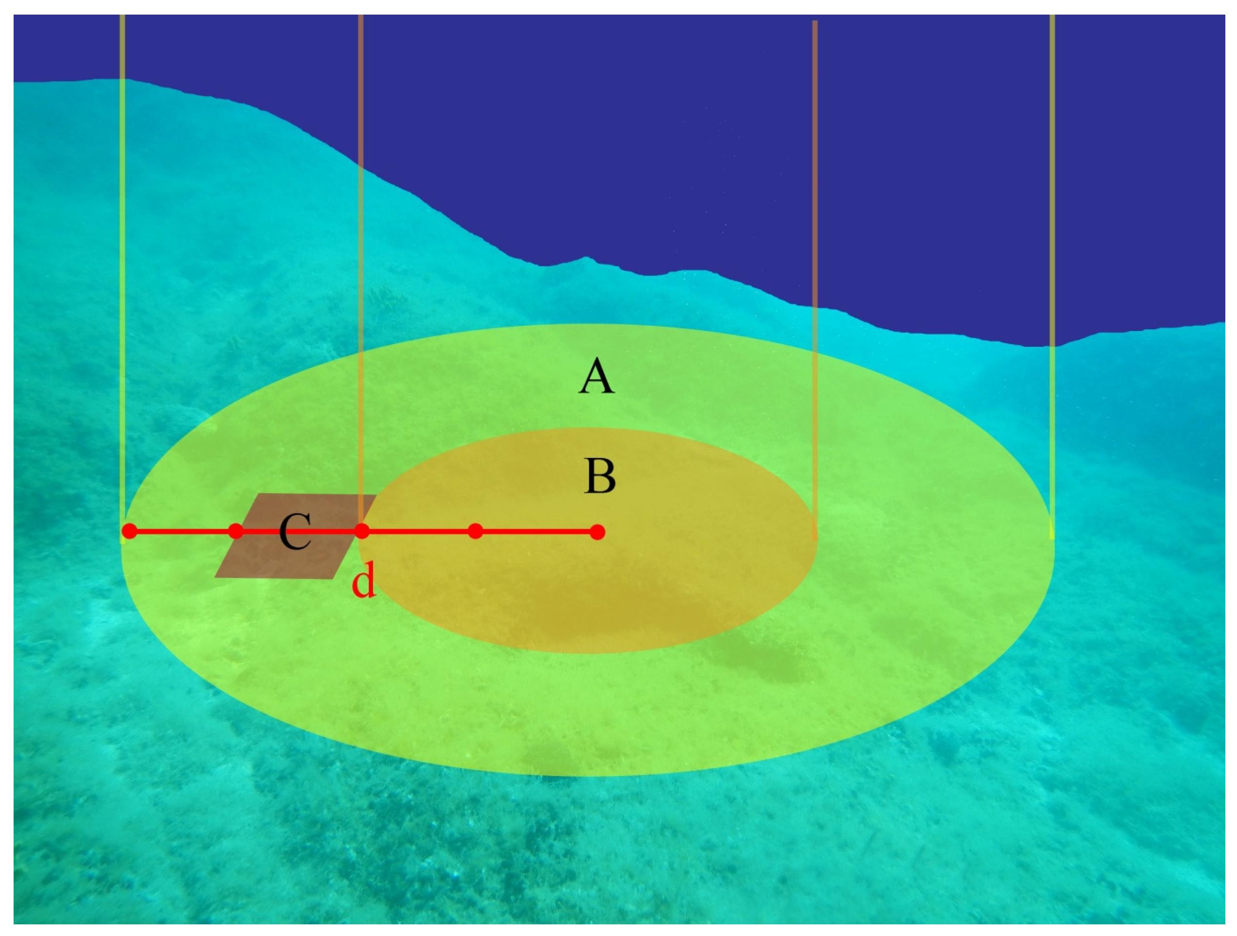
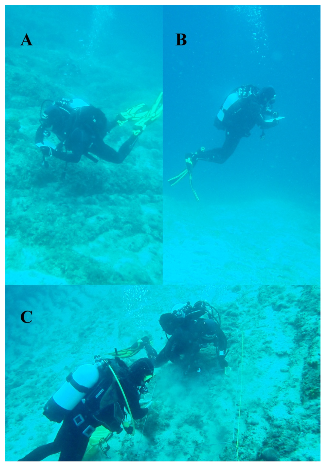
2.1. Study Area and Sampling Design

The study was carried out at three locations in the eastern Adriatic Sea in the Hvar Channel, two locations on Hvar island (Tatinja [TA], 43°13′5.7″ N, 16°38′21.7″ E, and Zala Luka [ZL], 43°13′6.06″ N, 16°39′2.76″ E) and one location on Brač island (Golubinja špilja [GO], 43°15′44.1″ N, 16°36′49.4″ E) (Figure 1).

Pretesting for the optimization of methods and equipment, and training of the divers in the procedure, were performed 8–12 October 2021. The data sampling was carried out 23–26 June 2022 and 11–17 October 2022. All dives were performed during the daytime between 10 am and 3 pm over eleven diving days. The two stationary visual census methods for fishes in cylinders [14] and the collecting of cryptobenthic fishes in squares saturated with anesthetics [9] were all applied at each of the randomly selected points using open-circuit SCUBA (Figure 2).

Two divers were included in the visual census and cryptobenthic fish collecting procedure (MK and IG), while the third diver (ZV in June and AS in October 2022) photographed and made video recordings. A total of 50 points were sampled, with 15 sampling points in June 2022 and 35 sampling points in October 2022. Roughly homogeneous (predominantly rocky flat bottom mixed with layers of different particle sizes) habitats between 5 and 15 m depth were chosen for sampling by simple random sampling using a predetermined pattern of random depths and distances (modified from [15]). The depths of sampling points were determined from 50 random integers ranging from 5 to 15. The distance between sampling points was based on 50 random integers ranging from 10 to 50 which were used as the number of determined swimming kicks. For the daily planned amount of sampling points, the random depths for each day were reordered to start with deeper points and end with the shallowest points to ensure safe diving within no decompression limits. The “Visibility to identify fish” (in meters) was assessed once at the beginning of each dive beneath the boat. A tape measure, with marks placed at every meter, was fixed and unwound until a fish larger than a total of 10 cm in length, located at the fixed starting point, could no longer be identified. The last distance at which the fish was still reliably identified, was considered the “Visibility to identify fish”, and it had to be a minimum of 4 m to proceed with the research. No dives were canceled due to low visibility reasons. During each dive, the initial point at the chosen depth was reached from the boat by the shortest route, perpendicular to the coastline. Subsequent points were reached by adjusting the depth from the previous point to the depth of the next point by the shortest route. This was followed by moving along the isobath in the correct direction, as viewed from the coast, using the number of swimming kicks determined from a table of random numbers. At each selected point, the first diver (MK) approached, laid down a tape measure representing radii of two and four meters, and performed stationary-census methods in cylinders (or point counts), following the modification of Bohnsack and Bannerot [15] by Minte-Vera et al. [14] (Figure 2). After the visual census, the second diver (IG) arrived with a square frame, fixing it between the 2nd and 3rd meter distance from the cylinder center to avoid the disturbed area beneath the diver during the visual census. Both divers then followed the modified protocol of Kovačić et al. [9] for collecting cryptobenthic fishes and recording habitat characteristics (Figure 2).

The visual census method employed in this study is based on the recommendations of Minte-Vera et al. [14], who proposed an enhanced visual census technique using sampling units composed of two nested cylinders with radii of 2 m and 4 m, respectively (Figure 2). This approach aimed to improve the accuracy and precision of estimates. Counts of small fish (species reaching approximately 10 cm in total length or less) were conducted within the smaller cylinder, while counts of larger fish (species exceeding 10 cm in total length) were made within the larger cylinder [14]. Given the challenge of estimating the size of each individual in species with higher abundance and determining whether each should be counted in the small or large cylinder, a size threshold was established for the entire species. In visual census studies with the intraspecific size as a studied variable, the size is usually roughly divided into three or four size classes. The threshold applied on each individual is almost impossible to perform more accurately, since the precision in underwater fish size estimation is 1–2 cm for fish around 10 cm size [14], and a number of fish of actual individual size around 10 cm would be wrongly assigned. Fish shoals of mixed sizes, i.e., with individuals larger and smaller than 10 cm length, would increase the error and confusion, especially large and fast-moving shoals. Minte Vera et al. [14] previously divided species into groups based on size and behavioral attributes. To delineate the plot areas for the stationary cylinders, a tape measure with marks at 2 and 4 m from the end was laid out (Supplementary Materials Video S1). The visual census commenced with the smaller cylinder of 2-m radius, focusing on smaller fishes that might attempt to escape or hide. Positioned at the end of the tape measure, i.e., at the center of the cylinder, the diver adopted a horizontal orientation to aim for a close-to-bottom view and less bottom disturbance by fins. During this process, both species and specimen counts were recorded (Figure 3A, Supplementary Materials Video S2). After inspection of the smaller cylinder, the diver identified fish in an upright position for the larger cylinder with a 4-m radius. All species within the cylinder were documented over a 5-min period (Figure 3B, Supplementary Materials Video S3). During this period, no counting was conducted for the larger cylinder except for highly mobile species that were unlikely to remain within the sampling area. Following the identification period for the larger cylinder, quantitative data were recorded for each species in a single 360° rotation. The number of fishes grouped in schools, equal to or greater than 8 individuals, was estimated using abundance classes based on multiples of 2:8, 16, 32, 64, 128, 256, etc. Body rotations were executed smoothly to minimize disturbance. Fish identification and counts were performed by a single diver (MK). MK has four decades of experience as a SCUBA diver and three decades of experience of underwater visual identification of fishes, including small benthic fishes, for environmental impact assessments and for scientific studies [13]. The species list and the abundance of each species were recorded on an acrylic slate. The identification of small species measuring less than 10 cm in total length followed the methods by Tiralongo [16] and Kovačić et al. [17]. The potential and limitations of visual census in identifying small benthic species, and of family Gobiidae in particular, were pointed out by Kovačić et al. [17], and we followed their recommendations about positive and provisional identifications of small benthic species from visual data, depending on the purposes of the identification.

The collection of cryptobenthic fishes and the recording of habitat characteristics were conducted using a modified protocol based on methods by Kovačić et al. [9] (Figure 3C). The sampling and documentation of each square followed a systematic protocol: (1) fixing a frame (1 × 1 m) onto the bottom (Supplementary Materials Video S4), (2) photographing the area as a reference for the recheck of habitat characteristics, (3) recording habitat characteristics, (4) spraying the anesthetic Quinaldine (Acros organics Bvba, Geel, Belgium) into the square, capturing escaping fishes with a hand net, and allowing approximately 2 min for the anesthetic to take effect (Supplementary Materials Video S5), and (5) removing movable parts of the bottom structure if present and collecting anesthetized fishes (Supplementary Materials Video S6). The frame was fixed between the 2nd and 3rd meter on the radius tape, i.e., out of the smaller cylinder with a 2 m radius (Figure 2). The anesthetic used was Quinaldine diluted to 1:15 with 96% ethanol and then mixed with sea water at 1:5 in 750-mL bottles. Typically, two bottles were used for each square, resulting in the use of a total volume of approximately 300 mL/m² of the Quinaldine-ethanol solution. Any fish initially observed as epibenthic within the frame at the beginning of the sampling, and later anesthetized, was not counted. These individuals were excluded from the cryptobenthic fish sampling and released. All collected cryptobenthic specimens were euthanized after SCUBA dives through over-anesthetization with Quinaldine and preserved in a 65% ethanol solution. Preliminary field species identifications of cryptobenthic specimens were subsequently rechecked in the laboratory on preserved specimens, and any necessary corrections to the data were made. Habitat characteristics, recorded separately for square and for cylinder areas, included depth measured in meters and inclination expressed in degrees calculated from the catheti, where the first cathetus was a 2-m rope fixed on the bottom and stretched horizontally, and the second cathetus was the height from the free end of the rope to the bottom (rounded to 0.25 m). The bottom substrate was categorized into five types based on estimated particle sizes, expressed as percentages of the total studied surface. Bottom layers were classified as no layers, a single layer of bottom particles (gravel to boulders), or multiple layers of bottom particles. Biocover included six types following the classification of Kovačić et al. [9]: phanerogams, long thallus algae, short thallus algae, calcareous algae, zoocover, no biocover. However, while the categories short thallus algae, calcareous algae, zoocover, and no biocover were recorded in this research, phanerogams and long thallus algae were absent.

2.2. Data Analysis

The fish assemblage dataset used in this analysis comprises sets of three different samplings collected at identical sampling points through distinct methods. The surface size of the studied points varied among methods, with the visual census method in cylinder with radius of 4 m (VCL) covering 50.27 m², the visual census method in cylinder with radius of 2 m (VCS) covering 12.57 m², and the collecting of cryptobenthic fishes in a square saturated with anesthetic (CB) covering 1 m² (Figure 2). This variation in the sampling area was attributed to the different methods employed, as detailed in the previous section. To standardize the comparison, total fish abundance and species abundance were recalculated to a standard unit of 1 m².

The recorded species count is highly influenced by the number of individuals sampled, which, in turn, varies based on the surface size of the studied point across methods. Therefore, the assessment of fish species richness between methods was performed using rarefaction analysis. Although different methods for rarefaction exist, in our case, sample size-based rarefaction and extrapolation of Hill numbers (q = 0) were utilized to generate accumulation curves, with associated 95% confidence intervals, using the iNEXT function from the iNEXT v2.0.20 R package [18]. The curves were rarefied/extrapolated up to twice the minimum sample size observed among the assessed methods. These extrapolations were based on samples pooled by location and season. Standard errors and confidence intervals were estimated for each method using 500 bootstrap replicates.

We began our analysis by examining the differences in fish total standardized abundance with univariate PERMANOVA tests [19], based on Euclidean distances, as the dataset did not meet ANOVA assumptions. This approach allowed us to assess whether the sampling methods (VCL, VCS, and CB) performed differently in detecting total fish abundance. Additionally, we applied the same analytical procedure to evaluate other variables of possible influence: various localities (ZL, TA, and GO), and different seasons (spring and autumn). Upon identifying significant effects among the evaluated factors, we extended our analysis by implementing a nested two-way PERMANOVA design. Here, Locality served as a fixed factor, with Method nested within Locality, enabling a more nuanced exploration of the Method’s impact while considering any Locality-related effects on the dependent variable. Subsequently, we conducted a post hoc pairwise nested comparison of Method by Locality to robustly quantify differences between distinct pairs of methods [20]. All procedures were carried out with 999 permutations.

To investigate differences in fish assemblage structure, species abundance (ln(x + 1) transformed) was compared using the same factors and levels as mentioned previously. Additionally, habitat variables (Depth, Inclination, Sand, Gravel, Cobbles, Boulders, Bedrock, Bottom layers, Short thallus algae, Calcareous algae, Zoocover, No biocover) were included as factors to assess potential habitat influences on fish assemblage structure among sampling points, despite the supposedly homogeneous habitat of a flattened bottom within a limited depth range of 5–15 m. For both sets of factors, one-way PERMANOVA, employing the Bray-Curtis distance measure, was applied, and statistical significance was determined using 999 permutations. Furthermore, a two-way PERMANOVA nested design was utilized for Method and Locality, where Method was nested in Locality, to further explore the significance of these two factors on species abundance. When significant effects were unveiled by two-way PERMANOVA nested tests, subsequent post hoc pairwise tests with 999 permutations were conducted for each locality [20]. However, it is important to note that the VCL and VCS methods inherently differ due to their defined targets, namely species maximum size exceeding (VCL) or falling below (VCS) 10 cm fish length, resulting in non-overlapping species compositions. As a result, only CB was subjected to testing against each of the other two methods (VCL and VCS). Subsequently, nonparametric multidimensional scaling (nMDS) plots [21] were generated using Bray-Curtis similarity matrices to visually depict the differences. The stress value, extracted from the nMDS, served as an indicator of the goodness of fit [22]. Following the PERMANOVA results, a two-way ANOSIM nested design was employed [23], where Method was nested in Locality, utilizing Bray–Curtis similarity on species abundance. Next, a post hoc pairwise test for CB against each of the other two methods (VCL and VCS) was conducted. Subsequently, we performed a similarity percentage analysis (SIMPER; [23]) to identify the species that contributed the most to the group dissimilarities previously identified by ANOSIM for Method nested in Locality. Finally, the species associated with each method were identified using an indicator species analysis function from the “indicspecies” R library [24]. This analysis facilitated the assessment of the association between each method and species through an Indicator Value constrained between 0 and 1, where higher values indicated stronger associations [25]. In all three analyses (ANOSIM, SIMPER, and indicator species analysis), as for PERMANOVA analysis on species abundance, only CB was subjected to testing against each of the other two methods (VCL and VCS).

The nMDS, ANOSIM, PERMANOVA and SIMPER analyses were carried out using the R software packages “vegan”, version 2.5-7. 2020 [26], and “pairwiseAdonis”, version 0.4 [20], for all pairwise comparison.

3. Results

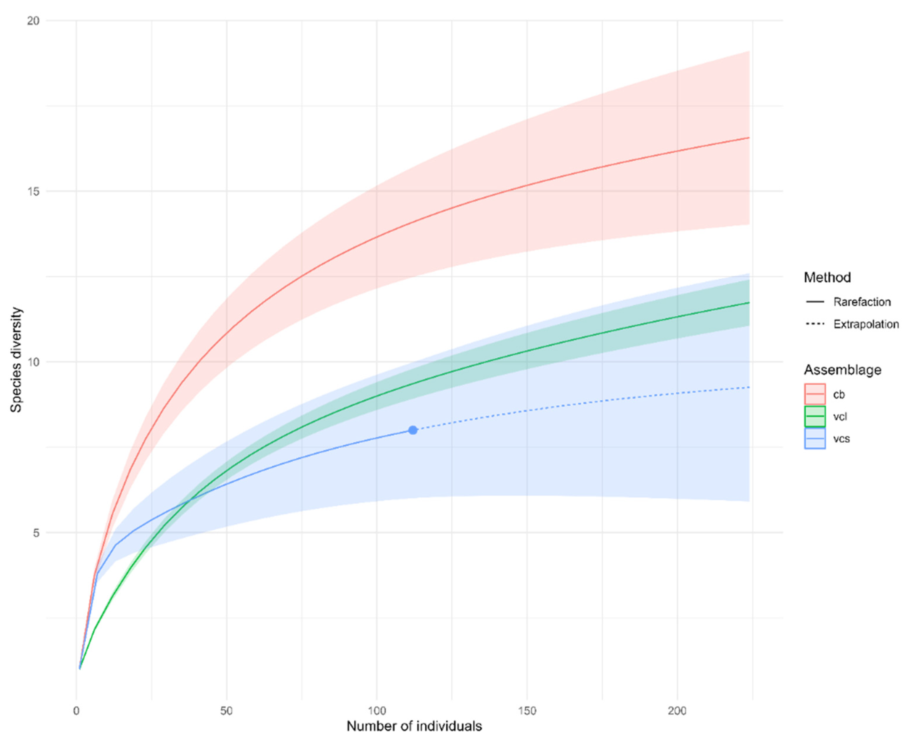
3.1. Diversity of Fish Species

The total number of recorded fish species from all three methods was 42. Specifically, the visual census methods accounted for 31 species, with 23 species recorded by the VCL method and 8 species by the VCS method (

Table 1. Recorded species from all three methods showing the number of specimens (see Section 2 for the counting method and surface size), abundance, and frequency of species occurrence at the points studied.

Species	Number of Individuals	Abundance (Individuals/m2)	Frequency of Occurrence (%)
Recorded species from the VCL method
Boops boops (Linnaeus, 1758)	96	0.0382	8%
Chromis chromis (Linnaeus, 1758)	2960	1.1783	94%
Coris julis (Linnaeus, 1758)	179	0.0713	98%
Diplodus annularis (Walbaum, 1792)	143	0.0569	26%
Diplodus puntazzo (Walbaum, 1792)	9	0.0036	14%
Diplodus sargus (Valenciennes, 1830)	4	0.0016	10%
Diplodus vulgaris (Geoffroy St. Hilaire, 1817)	110	0.0438	80%
Mullus surmuletus (Linnaeus, 1758)	3	0.0012	6%
Oblada melanura (Linnaeus, 1758)	17	0.0068	8%
Sarpa salpa (Linnaeus, 1758)	5	0.0020	6%
Scorpaena porcus (Linnaeus, 1758)	2	0.0008	6%
Seriola dumerili (Risso, 1810)	1	0.0004	4%
Serranus cabrilla (Linnaeus, 1758)	7	0.0028	14%
Serranus scriba (Linnaeus, 1758)	20	0.0080	30%
Sparus aurata (Linnaeus, 1758)	1	0.0004	4%
Spicara maena (Linnaeus, 1758)	45	0.0179	16%
Spicara smaris (Linnaeus, 1758)	96	0.0382	6%
Spondyliosoma cantharus (Linnaeus, 1758)	9	0.0036	12%
Symphodus cinereus (Bonnaterre, 1788)	1	0.0004	4%
Symphodus mediterraneus (Linnaeus, 1758)	9	0.0036	16%
Symphodus melanocercus (Risso, 1810)	1	0.0004	4%
Symphodus ocellatus (Forsskål, 1775)	16	0.0064	18%
Symphodus tinca (Linnaeus, 1758)	3	0.0012	8%
Recorded species from the VCS method
Gobius auratus (Risso, 1810)	30	0.0478	24%
Gobius fallax (Sarato, 1889)	19	0.0303	20%
Gobius geniporus (Valenciennes, 1837)	3	0.0048	8%
Gobius incognitus (Kovačić & Šanda, 2016)	1	0.0016	4%
Gobius roulei (de Buen, 1928)	2	0.0032	6%
Gobius vittatus (Vinciguerra, 1883)	31	0.0494	38%
Parablennius rouxi (Cocco, 1833)	25	0.0398	32%
Tripterygion delaisi (Cadenat & Blache, 1970)	1	0.0016	4%
Recorded species from the CB method
Chromis chromis (Linnaeus, 1758)	6	0.12	10%
Chromogobius zebratus (Kolombatović, 1891)	6	0.12	12%
Corcyrogobius liechtensteini (Kolombatović, 1891)	18	0.36	18%
Marcelogobius splechtnai (Ahnelt & Patzner, 1995)	3	0.06	6%
Gaidropsarus mediterraneus (Linnaeus, 1758)	1	0.02	4%
Gobius auratus (Risso, 1810)	7	0.14	12%
Gobius fallax (Sarato, 1889)	15	0.3	22%
Gobius vittatus (Vinciguerra, 1883)	26	0.52	36%
Grammonus ater (Risso, 1810)	1	0.02	4%
Lepadogaster candolii (Risso, 1810)	6	0.12	12%
Millerigobius macrocephalus (Kolombatović, 1891)	19	0.38	26%
Odondebuenia balearica (Pellegrin and Fage, 1907)	135	2.7	80%
Parablennius rouxi (Cocco, 1833)	7	0.14	14%
Scorpaena notata (Rafinesque, 1810)	2	0.04	6%
Symphodus ocellatus (Forsskål, 1775)	1	0.02	4%
Thorogobius macrolepis (Kolombatović, 1891)	1	0.02	4%
Tripterygion delaisi (Cadenat & Blache, 1970)	4	0.08	8%
Zebrus zebrus (Risso, 1827)	72	1.44	68%

). On average, the species richness of the VCL method was 4.5 species per cylinder, while the VCS method yielded an average species richness of 1.2 species per cylinder. Additionally, the collection of cryptobenthic fishes in squares using anesthetic (CB) resulted in 18 species, with an average species richness of 3.1 species per square (Table 1). The rarefaction analysis showed non-overlapping confidence intervals between the lower species diversity estimated for VCL and VCS methods and the higher species diversity of CB method (Figure 4). The species richness of VCL and VCS methods showed no significant difference (Figure 4). The diversities of all methods were rarefied to the lowest number of observed individuals per method (112 individuals in VCS), providing the possibility of comparing the higher species richness numbers of the CB method versus VCL and VCS methods (Figure 4,

Table 2. Estimated species richness (q = 0) for twice the lowest number of observed individuals per method (2 × 112 individuals in VCS). Method abbreviations (VCL, VCS, CB) explained in the text; m—sample size, SC—sample coverage estimate for the reference sample, qD—based diversity, qD.LCL—lower limits and qD.UCL—upper limits of the 95% confidence interval.

Method	m	SC	qD	qD.LCL	qD.UCL
VCL	224	0.923	11.7	11.0	12.4
VCS	224	0.994	9.26	5.5	13.1
CB	224	0.924	16.6	14.2	12.9

). All species recorded by VCL, except Scorpaena porcus (Linnaeus, 1758), were hyperbenthic or benthopelagic (Table 1). The species recorded by VCS were exclusively found at the bottom, both results suggesting that VCS is well-suited for capturing epibenthic fishes, whereas VCL appears better suited for hyperbenthic or benthopelagic species. Among the eight epibenthic species recorded by VCS, five were also observed in squares where anesthetic was used to collect hidden species, indicating their ambivalent or epicryptobenthic nature (Table 1). Two species were recorded by both VCL and CB methods, including Chromis chromis (Linnaeus, 1758) and Symphodus ocellatus (Forsskål, 1775) (Table 1). C. chromis exhibited both cryptobenthic and benthopelagic occurrences, while a single solitary juvenile of the usually hyperbenthic S. ocellatus was observed hidden within bottom spaces.

3.2. Total Fish Abundance

The one-way PERMANOVA indicated a significant difference in the total abundance among methods and localities, with no significant difference between seasons (

Table 3. Summary of PERMANOVA results for assessing differences in total fish abundance among methods, sites and seasons: (a) one-way PERMANOVA, (b) Method nested within Locality, (c) post-hoc pairwise comparison with Method nested within Locality. Method abbreviations (VCL, VCS, CB) explained in the text. Significant values marked: * p < 0.05; *** p < 0.001.

Source of Variation	Df	MS	Pseudo-F	p (Perm)
(a)
Locality	2	0.251	2.825	0.0317 *
Method	2	7.137	80.236	0.0001 ***
Season	1	0.226	3.034	0.0508
(b)
Locality	2	0.513	2.313	1 × 10−4 ***
Locality: Method	6	2.467	27.71	1 × 10−4 ***
(c)
Locality: Method, CB vs. VCS	5	2.706	42.965	1 × 10−4 ***
Locality: Method, CB vs. VCL	5	0.842	9.0415	1 × 10−4 ***
Locality: Method, VCS vs. VCL	5	1.241	11.265	1 × 10−4 ***

). The influences of Method and Locality were separated by the nested two-way PERMANOVA, with methods nested within localities. The two-way PERMANOVA’s nested design, with Method nested in Locality, revealed again a significant effect of Locality, as well as a significant effect of Method nested within Locality (Table 3). Furthermore, in the pairwise nested comparison of Method by Locality, each method again had significantly different fish abundance compared to the other two methods (Table 3). The VCL method exhibited no empty records, with the estimated number of all fish individuals ranging at each point from 4 to 272, and an average of 74.74 ± 74.87 (mean ± standard deviation) individuals for the cylinder, equivalent to 1.49 individuals/m² for the bottom surface of the cylinder. The VCS method had 12 empty recording points and recorded the number of all fish individuals in cylinders, with fish recorded ranging from 1 to 16, resulting in an average of 2.24 ± 2.77 (mean ± standard deviation) individuals for the cylinder, representing only 0.18 individuals/m² for the bottom surface. The CB method collected 330 individuals in a total surface of 50 m², providing an average density of 6.6 ± 2.86 individuals/m² (mean ± standard deviation) and ranging from 1 to 15 individuals/m², with no empty squares. Surprisingly, cryptobenthic fishes from squares exhibited higher abundance compared to both visual census methods. The weak result of the VCS method could be attributed to the lack of rugosity in the targeted homogeneous flattened habitats and shallow water depth of 5 to 15 m on a relatively exposed coast, as all recorded fish species of less than 10 cm size were epibenthic, depending on bottom complexity for food and shelter. Conversely, the abundance of cryptobenthic fishes was surprisingly large and unexpected, considering the same limitations of the bottom type. The risk of epibenthic individuals escaping to shelter when disturbed and counted as cryptobenthic was possible, but hardly influential, given that: (1) any anesthetized fish observed in the square frame as originally epibenthic were excluded from the cryptobenthic fish sampling, (2) the surfaces of the square and narrow cylinder were not overlapping (Figure 2), and (3) the VCS method, in general, showed poor abundance compared to the CB method, particularly for the ambivalent or epicryptobenthic species, which ranged from 0.0016 to 0.0478 individuals/m² for species in VCS versus 0.14 to 0.52 individuals/m² for the same species from CB sampling (Table 1).

3.3. Fish Assemblage Structure and Fish Species Abundance and Frequency

The one-way PERMANOVA tests conducted on species abundance concerning habitat factors revealed that, despite the deliberate selection of a relatively homogeneous flattened bottom within a narrow depth range of 5 to 15 m for this study, both bottom depth and the extent of bedrock surface still exerted significant influence on the fish assemblage structure (

Table 4. Summary of PERMANOVA results for species abundance: (a) one way PERMANOVA assessing differences across different habitat factors, (b) one-way PERMANOVA assessing differences among methods, sites and seasons, (c) Method nested within Locality, (d–f) post-hoc pairwise comparison of Method for each Locality separately. Method abbreviations (VCL, VCS, CB) explained in the text. Significant values marked: * p < 0.05; ** p < 0.01, *** p < 0.001.

Source of Variation	Df	MS	Pseudo-F	p (Perm)
(a)
Depth	1	0.011	3.105	0.010 **
Inclination	1	0.006	1.773	0.105
Sand	1	0.004	1.113	0.343
Gravel	1	0.004	1.271	0.249
Cobbles	1	0.004	1.137	0.334
Boulders	1	0.005	1.439	0.192
Bedrock	1	0.009	2.582	0.025 *
Bottom layers	1	0.005	1.243	0.279
Short thallus algae	1	0.002	0.513	0.827
Calcareous algae	1	0.099	1.288	0.222
Zoocover	1	0.006	1.774	0.091
No biocover	1	0.005	1.627	0.131
(b)
Locality	2	0.039	5.437	0.001 ***
Method	2	0.471	65.695	0.001 ***
Season	1	0.005	1.450	0.173
(c)
Locality	2	0.041	5.981	0.001 ***
Locality: Method	6	0.516	25.028	0.001 ***
(d) ZL
Locality: Method, CB vs. VCS	1	0.266	11.576	0.001 ***
Locality: Method, CB vs. VCL	1	0.559	43.133	0.001 ***
(e) TA
Locality: Method, CB vs. VCS	1	0.294	12.914	0.001 ***
Locality: Method, CB vs. VCL	1	0.618	54.996	0.001 ***
(f) GO
Locality: Method, CB vs. VCS	1	0.372	11.271	0.001 ***
Locality: Method, CB vs. VCL	1	0.640	46.405	0.001 ***

).

The one-way PERMANOVA tests conducted on species abundance revealed a significant distinction in fish assemblage structure among methods and localities (Table 4). Interestingly, no significant variations were observed in the fish assemblage structure between the spring and autumn seasons. Given the high significance of both Method and Locality as factors, a nested two-way PERMANOVA was employed with Method nested within Locality to distinguish the influence of methods and localities. The results of this test reaffirmed the significant differences in fish assemblage structure among methods (Table 4). Additionally, in pairwise comparisons of CB against each of the other two methods (VCL and VCS), performed separately for each locality, CB exhibited significantly distinct fish assemblages at all three localities compared to the two visual census methods (Table 4). The visual census methods displayed non-overlapping fish assemblages between them by default (see Section 2). These findings underscore the complementary nature of all three methods, as they target different components of fish assemblages within the same habitat.

The nMDS plot effectively illustrates the differentiation in fish assemblage species composition among different methods (Figure 5), corroborating our findings. Furthermore, the two-way ANOSIM nested design, with Method nested within Locality, revealed a significant effect size of methods on fish assemblage structure, consistent with the significant differences in fish assemblage structure among methods identified by PERMANOVA (

Table 5. Summary of ANOSIM results for species abundance: 2-way nested ANOSIM, Method nested within Locality and post-hoc pairwise comparison with Method nested within Locality. Method abbreviations (VCL, VCS, CB) explained in the text. Significant values marked: *** p < 0.001.

	R Value	p
Locality: Method	0.780	1 × 10−4 ***
Locality: Method, CB vs. VCS	0.546	1 × 10−4 ***
Locality: Method, CB vs. VCL	0.921	1 × 10−4 ***

). Given the inherent difference in fish assemblage structure between VCL and VCS, only the pairs of CB against VCL and CB against VCS were individually tested using the ANOSIM nested design, where Method was nested in Locality. Both pairs demonstrated a significant effect of methods on fish assemblage structure (Table 5), thereby reinforcing the findings from the PERMANOVA analysis.

The most abundant fish of VCL was, by far, C. chromis, with 1.18 individuals/m² (Table 1). The second most abundant fish, hyperbenthic Coris julis (Linnaeus, 1758), had about 1/16 the abundance of C. chromis (Table 1). Many more fish species with an abundance above 0.1 individuals/m² were recorded by the CB method compared to the VCL method. Ten species had more than 0.1 individuals/m², with cryptobenthic generalists Odondebuenia balearica (Pellegrin and Fage, 1907) and Zebrus zebrus (Risso, 1827), having an astonishing 2.7 and 1.44 individuals/m², respectively (Table 1). The gobies Gobius auratus (Risso, 1810) and Gobius vittatus (Vinciguerra, 1883), the most abundant fishes of VCS, were more than one order of magnitude less abundant than the most abundant fishes in the other two methods (Table 1). The high abundance of strict cryptobenthic gobiid species, and much lower abundance of small epibenthic gobiid species, as well as the predominance of cryptobenthic individuals in ambivalent species, are the most surprising species abundance results of this research. These findings can be also explained by the lack of rugosity in the studied homogeneous flattened habitats, forcing the exposed individual to hide more in hidden bottom spaces.

In the SIMPER analysis, again, given the inherent difference in fish assemblage structure between VCL and VCS, only the pairs of CB against VCL and CB against VCS results were taken into account. The two most abundant species in VCL had the highest contribution to dissimilarity of VCL to CB species composition. Both species are, in relation to the bottom, hyperbenthic (

Table 6. Results of similarity percentages procedure (SIMPER) analysis with Method nested within Locality showing fish species contributing most (in order of decreasing percentage) to dissimilarity among methods. Method abbreviations (VCL, VCS, CB) explained in the text.

CB vs. VCS		CB vs. VCL
Species	%	Species	%
Odondebuenia balearica	24.2	Chromis chromis	30.1
Zebrus zebrus	15.5	Coris julis	14.0
Gobius vittatus	11.0	Odondebuenia balearica	10.5
Parablennius rouxi	8.8	Diplodus vulgaris	8.7
Gobius auratus	7.7	Zebrus zebrus	6.8
Gobius fallax	6.7	Gobius vittatus	2.8
Millerigobius macrocephalus	4.2	Diplodus annularis	2.5
Corcyrogobius liechtensteini	3.0	Millerigobius macrocephalus	2.0
Chromogobius zebratus	1.6	Serranus scriba	1.9
Lepadogaster candolii	1.5	Spicara maena	1.8

). Between CB and VCS, two exclusively cryptobenthic species had the highest contribution to species composition dissimilarity, followed by the three ambivalent species present in both methods (Table 6). The Indicator species analysis showed hyperbenthic species as a significant indicator for the VCL method, exclusively cryptobenthic species as a significant indicator for the CB method, if compared to VCS, and combination of cryptobenthic and ambivalent species, if compared to VCL, and ambivalent species as a significant indicator for the VCS method (

Table 7. Results of Indicator species analysis with the significant indicator fish species for each method. Method abbreviations (VCL, VCS, CB) explained in the text. Significant values marked: * p < 0.05; ** p < 0.01, *** p < 0.001.

Species	Indicator Value	p
VCL
Coris julis	0.900	0.0001 ***
Chromis chromis	0.848	0.0001 ***
Diplodus vulgaris	0.725	0.0001 ***
Serranus scriba	0.382	0.0001 ***
Symphodus mediterraneus	0.267	0.0114 *
Diplodus annularis	0.253	0.0004 ***
Serranus cabrilla	0.248	0.0270 *
Symphodus ocellatus	0.247	0.0200 *
Diplodus puntazzo	0.233	0.0257 *
Spicara maena	0.227	0.0137 *
CB (vs. VCL)
Odondebuenia balearica	0.732	0.0001 ***
Zebrus zebrus	0.651	0.0001 ***
Gobius vittatus	0.423	0.0001 ***
Millerigobius macrocephalus	0.352	0.0003 ***
Gobius fallax	0.320	0.0019 **
Corcyrogobius liechtensteini	0.270	0.0054 **
Parablennius rouxi	0.248	0.0286 *
VCS
Parablennius rouxi	0.335	0.0018 **
Gobius auratus	0.260	0.0110 *
CB (vs. VCS)
Odondebuenia balearica	0.732	0.0001 ***
Zebrus zebrus	0.651	0.0001 ***
Millerigobius macrocephalus	0.352	0.0009 ***
Corcyrogobius liechtensteini	0.270	0.0098 **

). The SIMPER and the Indicator species analysis specified the species that shape each of the distinct components of fish assemblages found to be different by the PERMANOVA and ANOSIM analyses.

The most frequent fishes of VCL were, similarly to abundance, C. julis and C. chromis, present in 98% and 94% of larger cylinders, respectively (Table 1). The species frequency of occurrence is not comparable between methods, due to a different studied surface size for the methods (50.24 m² of the bottom surface for the larger cylinder, 12.56 m² of the bottom surface for the smaller cylinder, and 1 m² bottom surface squares). VCS showed a much lower frequency of species occurrence compared to large cylinders, with G. vittatus and Parablennius rouxi (Cocco, 1833) being the most frequent species, occurring in 38% and 32% of the smaller cylinders, respectively (Table 1). The most frequent fishes of the CB method with the application of anesthetic were, similarly to abundance, O. balearica and Z. zebrus, present in 80% and 68% of squares, respectively (Table 1).

Nearly half of all fish species recorded by VCL were Sparidae, with eleven species, followed by Labridae with six species. Another five fish families had only one or two representatives in this census method. However, due to the abundance of C. chromis, Pomacentridae was the most abundant fish family in VCL, and together with Sparidae, comprised 93.5% of all individual fish (Table 1). The fish recorded by VCS were predominantly Gobiidae, with six out of eight species and 76.8% of all individuals being gobies, while one blenniid and one tripterygid species were also recorded (Table 1). Among cryptobenthic fishes from the CB method, Gobiidae was again predominant, with ten species and 91.5% of all recorded individuals being gobies, while for the other eight species each belonged to a different fish family (Table 1). Since the species recorded in VCS were all recorded at the bottom, it can be concluded that the entire bottom epibenthic and cryptobenthic fish fauna was dominated by Gobiidae, both in the sense of species richness and of fish abundance.

4. Discussion

The current findings reveal a lower total fish species richness compared to two other studies of Mediterranean reef fishes, which also utilized a combination of methods including visual census and anesthetic application [12,13]. While Mazzoldi and De Girolamo [12] and Soldo et al. [13] employed similar qualitative methods, focusing on visual census and anesthetic application, our research emphasizes an integrative approach aimed at quantitatively comparing these methods. However, it is worth noting that Mazzoldi and De Girolamo [12] conducted extensive sampling across numerous localities along the coast of Lampedusa island, and Soldo et al. [13] studied submerged cliffs across a wide depth range, targeting diverse depth zones and different fish communities. In contrast, the present study focused on homogeneous flattened habitats and shallow waters (5 to 15 m depth) along a relatively exposed coast, potentially contributing to the lower species richness observed.

The homogeneous flattened habitats targeted in our research also likely account for the low abundance and species richness of epibenthic fishes compared to earlier studies. For instance, in our results, epibenthic fish exhibited a density of 0.18 individuals/m² and 8 species, contrasting with 0.88 individuals/m² and 14 species reported by Kovačić et al. [9], 1.22 individuals/m² and 8 species by Glavičić et al. [27], and 0.38 individuals/m² and 13 species by Glavičić et al. [28]. The only exception is a study conducted inside a marine cave [29], where the low abundance is understandable due to decreased food resources in such habitats. It is important to note that our VCS method covered a surface area of 12.57 m² per point, while the count of epibenthic fish in all those previous studies were performed over a 1 m² square surface.

The unexpectedly high abundance and species richness of cryptobenthic fishes recorded in our study, despite the habitat limitations, align well with earlier quantitative studies of Mediterranean cryptobenthic fishes. For instance, our results revealed a density of 6.6 individuals/m² and 18 species, while Kovačić et al. [9] reported 6.86 individuals/m² and 24 species, Glavičić et al. [27] reported 6.64 individuals/m² and 19 species, Glavičić et al. [28] reported 2.92 individuals/m² and 22 species, and Kovačić et al. [29] reported 3.58 individuals/m² and 9 species. Notably, our research showed a cryptobenthic/epibenthic individuals ratio of 36.7 to 1, favoring cryptobenthic individuals, which contrasts with the ratios of 5.4–7.8 to 1 observed in earlier studies, except for the marine cave study where Kovačić et al. [29] reported a ratio of 32.5 to 1. Gobiidae emerged as the fish family with the highest species richness and abundance among both epibenthic and cryptobenthic fishes, underscoring their dominant role in shaping the bottom and in-bottom fish communities. It is worth noting that the high cryptobenthic fish density, prevailing over epibenthic or hyperbenthic fish abundance, observed in our study and in other studies in the Eastern Adriatic, raises questions about whether similar patterns also exist in other Mediterranean regions. Further studies in other Mediterranean areas could provide insights into the broader distribution of high cryptobenthic fish density observed along the Eastern Adriatic littoral.

Regarding individual species, the high abundance and frequency of occurrence of strictly cryptobenthic gobiid species, especially cryptobenthic generalists, O. balearica and Z. zebrus, and a far lower abundance of small epibenthic gobiid species, as well as the predominance of cryptobenthic individuals in ambivalent species, is the most surprising species abundance result of this research (Table 1). This disparity can be attributed to the lack of rugosity in the homogeneous flattened habitats we studied, compelling otherwise exposed individuals to seek refuge from predators or wave action in hidden bottom spaces. Odondebuenia balearica and Z. zebrus are two cryptobenthic species with a limited records just two decades ago. The quantitative studies published later found these species, together with Corcyrogobius liechtensteini (Kolombatović, 1891), to be the most frequent and abundant cryptobenthic fishes, with O. balearica only being rare in very shallow water (<3 m depth) and Z. zebrus only avoiding the deeper bottom (>20 m depth) [9,27,28,29]. The behavior of C. chromis also aligns with previous observations regarding its utilization of cryptic spaces, even as an adult and during the daytime [9,27]. The species is obviously a switcher between hidden spaces and the water column, having a unique cryptobenthic/benthopelagic combination of behavior among studied species [28]. In the VCL method, C. chromis and C. julis were overwhelmingly abundant and frequent (Table 1). The prevalence of these species among fishes occurring over rocky and mixed bottoms in the Mediterranean has already been observed in other published visual census studies [30,31,32]. Furthermore, at least one of these species, including C. chromis [33,34] or C. julis, together with Thalassoma pavo (Linnaeus, 1758) [35], were also observed as the most abundant in some research studies. In the study by Bell [36], C. chromis was the most abundant at deeper sites, together with Boops boops (Linnaeus, 1758), and C. julis at shallow sites.

A striking rarity or absence of small epibenthic and cryptobenthic species can be found in the published Mediterranean visual censuses. Checking ten random visual census papers covering the Mediterranean area from Spain to Greece in the last forty years, (1) where results were based only on the visual census methods, (2) where the species list was presented in the paper, and (3) which were highly cited, i.e., with >50 citations (>20 if published in the last decade) on ResearchGate [37], species of less than 10 cm in length represented only 0% to 15.2% of total species richness (

Table 8. Percentage of cryptobenthic and small (≤10 cm) epibenthic species in the total fish species richness in the present study, in two papers with qualitatively combined data, and in the randomly selected visual census papers. * Species recorded in both categories counted once.

Reference	Number of Identified Cryptobenthic Species	Number of Identified Small (≤10 cm) Epibenthic Species	Both Categories Sum as the Percentage of the Total Recorded Species Richness *
Visual census studies
Bell [36]	0	2	5.7%
Harmelin [30]	0	7	14.9%
Francour et al. [31]	0	5	15.2%
Guidetti [32]	0	4	11.8%
De Girolamo & Mazzoldi [35]	0	6	25.0%
Ordines et al. [39]	0	0	0.0%
García-Charton & Pérez-Ruzafa [33]	0	0	0.0%
Orlando-Bonaca & Lipej [38]	0	11	29.7%
Azzurro et al. [34]	0	6	14.3%
Giakoumi & Kokkoeis [40]	0	0	0.0%
Studies with qualitatively combined data
Mazzoldi and De Girolamo [12]	6	14	26.0%
Soldo et al. [13]	22	13	39.4%
Present research	18	8	45.2%

). An exception to this general pattern is observed in the studies conducted by De Girolamo & Mazzoldi [35] and Orlando-Bonaca & Lipej [38]. In De Girolamo & Mazzoldi [35], the representation of species less than 10 cm in size accounted for a quarter of the total species richness. This higher representation can be attributed to the separate visual censuses performed for fishes on the bottom and those swimming or hovering above it. Similarly, the meticulous visual census conducted in shallow waters (0.5–3 m depth) by Orlando-Bonaca & Lipej [38] managed to capture a diverse range of shallow water blenniids, resulting in these smaller species representing an average of 29.7% of the total species richness. In the combined data of Mazzoldi and De Girolamo [12] and Soldo et al. [13], species smaller than 10 cm in size represented 26.0% and 39.4% of the total species richness, respectively (Table 8). Remarkably, in the present study, these smaller species accounted for 45.2% of the total species richness (Table 8). It could be hypothesized that the studies involving cryptobenthic fishes and having a high diversity of small benthic species have been performed in areas where small fishes are more prevalent than elsewhere in the Mediterranean, contrary to the previously mentioned visual census studies. Indeed, one of the authors (MK, unpublished data) noticed through his Adriatic and Mediterranean diving experience that small epibenthic and cryptobenthic fishes are much more common at depths of 0–20 m in sheltered sea canals among the islands of the Eastern Adriatic and of the Aegean Sea, than on the exposed Mediterranean coasts. Again, as for cryptobenthic fish density, only similar studies in other Mediterranean areas could answer the question of whether the rest of the shallow water Mediterranean coasts contain a high density of small benthic fish like the Eastern Adriatic littoral. However, it is worth noting that the combined study of Mazzoldi and De Girolamo [12] and the visual census of two different speeds conducted by De Girolamo and Mazzoldi [35] were both carried out in Lampedusa, while Guidetti’s [32] visual census was performed in the Adriatic Sea (Table 8), bringing into question eventual geographic differences.

The present quantitative comparison of methods of visual census and cryptobenthic fish collection showed significantly different species richness (except between VCL and VCS), total fish abundance, and fish assemblage structure (not tested for VCL vs. VCS) among methods. Two methods, VCS and CB, did not share or barely shared recorded species with VCL. The VCS and CB methods were therefore complementary to the present VCL method, which mostly resembled the usually applied visual census method, such as various transects methods [12,13]. Furthermore, despite both methods recording ambivalent species, each of them in one habitat position, the VCS and CB methods also exhibited clear differences from one another. The two cylinder methods were originally designed for visual census of fishes of different sizes [14]. However, our findings suggest a nearly complete size split between epibenthic fishes and hyperbenthic/benthopelagic fishes. As a result, the cylinder with a 2 m radius was well-suited for recording epibenthic fishes, while the cylinder with a 4 m radius was reliable for hyperbenthic and benthopelagic fishes, with the diver’s position and movement adjusted in each of the methods. In the present study, the diver most experienced in identification of small benthic fishes was selected for the task of fish identification. We think that the diver effect should be researched by a standalone study for the present method of a cylinder with a 2 m radius, as well as for any other visual census method that could be developed for the same purpose, considering the problem of the visual identification of small benthic fishes [17]. Other quantitative methods will likely be developed for each of the three benthic fish components (cryptobenthic, epibenthic, and hyperbenthic fishes) based on the fish habitat positioning, as defined by Kovačić et al. [9], and hopefully, these methods will be quantitatively comparable and integrated together as are methods in the present research.

5. Conclusions

We recommend the combination of the three separate methods for the three benthic fish components, as they collectively represent the entirety of the fish littoral benthos. This integrative approach provides the most accurate and comprehensive assessment of the Mediterranean temperate reef fish assemblage, offering valuable insights into its qualitative and quantitative composition.

References

1. Watson, D.L.; Harvey, E.S.; Anderson, M.J.; Kendrick, G.A. A comparison of temperate reef fish assemblages recorded by three underwater stereo-video techniques. Mar. Biol. 2005, 148, 415–425. [Google Scholar] [CrossRef]
2. Brock, V.E. A preliminary report on a method of estimating reef fish populations. J. Wildl. Manag. 1954, 18, 289–308. [Google Scholar] [CrossRef]
3. Harmelin-Vivien, M.L.; Harmelin, J.G. Présentation d’une méthode d’évaluation in situ de la faune ichtyologique. Parc Natl. Port-Cros Trav. Sci. Port-Cros 1975, 1, 47–52. [Google Scholar]
4. Harmelin-Vivien, M.L.; Harmelin, J.G.; Chauvet, C.; Duval, C.; Galzin, R.; Lejeune, P.; Barnabe, G.; Blanc, F.; Chevalier, R.; Duclerc, J.; et al. Evaluation visuelle des peuplements et populations de poissons méthodes et problèmes. Rev. Écol. (Terre Vie) 1985, 40, 467–539. [Google Scholar] [CrossRef]
5. Brock, R.E. A critique of the visual census method for assessing coral reef fish populations. Bull. Mar. Sci. 1982, 32, 269–276. [Google Scholar]
6. Ackerman, J.L.; Bellwood, D.R. Reef fish assemblages: A reevaluation using enclosed rotenone stations. Mar. Ecol. Prog. Ser. 2000, 206, 227–237. [Google Scholar] [CrossRef]
7. Willis, T. Visual census methods underestimate density and diversity of cryptic reef fishes. J. Fish Biol. 2001, 59, 1408–1411. [Google Scholar] [CrossRef]
8. Smith-Vaniz, W.F.; Jelks, H.L.; Rocha, L.A. Relevance of cryptic fishes in the biodiversity assessments: A case study at Buck Island Reef National Monument, St. Croix. Bull. Mar. Sci. 2006, 79, 17–48. [Google Scholar]
9. Kovačić, M.; Patzner, R.A.; Schliewen, U.K. A first quantitative assessment of the ecology of cryptobenthic fishes in the Mediterranean Sea. Mar. Biol. 2012, 159, 2731–2742. [Google Scholar] [CrossRef]
10. Alzate, A.; Zapata, F.A.; Giraldo, A. A comparison of visual and collection-based methods for assessing community structure of coral reef fishes in the Tropical Eastern Pacific. Rev. Biol. Trop. 2014, 62 (Suppl. S1), 359–371. [Google Scholar] [CrossRef]
11. Beldade, R.; Goncalves, E.J. An interference visual census technique applied to cryptobenthic fish assemblages. Vie Milieu 2007, 57, 61–65. [Google Scholar]
12. Mazzoldi, C.; De Girolamo, M. Littoral fish community of the Island Lampedusa (Italy): A visual census approach. Ital. J. Zool. 1998, 65 (Suppl. S1), 275–280. [Google Scholar] [CrossRef]
13. Soldo, A.; Glavičić, I.; Kovačić, M. Combining Methods to Better Estimate Total Fish Richness on Temperate Reefs: The Case of a Mediterranean Coralligenous Cliff. J. Mar. Sci. Eng. 2021, 9, 670. [Google Scholar] [CrossRef]
14. Minte-Vera, C.V.; de Moura, R.L.; Francini-Filho, R.B. Nested sampling: An improved visual-census technique for studying reef fish assemblages. Mar. Ecol. Prog. Ser. 2008, 367, 283–293. [Google Scholar] [CrossRef]
15. Bohnsack, J.A.; Bannerot, S.P. A Stationary Visual Census Technique for Quantitatively Assessing Community Structure of Coral Reef Fishes; NOAA Technical Report NMFS; U.S. Department of Commerce, National Technical Information Service: Springfield, VA, USA, 1986; Volume 41, pp. 1–15.
16. Tiralongo, F. Blennies of the Mediterranean Sea: Biology and identification of Blenniidae, Clinidae, Tripterygiidae; Amazon Fulfillment Poland Sp. z o.o.: Wroclaw, Poland, 2020; p. 131. [Google Scholar]
17. Kovačić, M.; Renoult, J.P.; Pillon, R.; Svensen, R.; Bogorodsky, S.V.; Engin, S.; Louisy, P. Identification of Mediterranean marine gobies (Actinopterygii: Gobiidae) of the continental shelf from photographs of in situ individuals. Zootaxa 2022, 5144, 1–103. [Google Scholar] [CrossRef] [PubMed]
18. Hsieh, T.C.; Ma, K.H.; Chao, A. iNEXT: An R package for rarefaction and extrapolation of species diversity (Hill numbers). Methods Ecol. Evol. 1987, 7, 1451–1456. [Google Scholar] [CrossRef]
19. Anderson, M.J. A new method for non-parametric multivariate analysis of variance. Austral Ecol. 2001, 26, 32–46. [Google Scholar]
20. Martinez Arbizu, P. pairwiseAdonis: Pairwise multilevel comparison using adonis. R Package Version 001. 2017. Available online: https://github.com/pmartinezarbizu/pairwiseAdonis (accessed on 1 December 2017).
21. Field, J.G.; Clarke, K.R.; Warwick, R.M. A practical strategy for analysing multispecies distribution pattern. Mar. Ecol. Prog. Ser. 1982, 8, 37–52. [Google Scholar] [CrossRef]
22. Dexter, E.; Rollwagen-Bollens, G.; Bollens, S.M. The trouble with stress: A flexible method for the evaluation of nonmetric multidimensional scaling. Limnol. Oceanogr. Methods 2018, 16, 434–443. [Google Scholar] [CrossRef]
23. Clarke, K.R. Non-parametric multivariate analyses of changes in community structure. Aust. J. Ecol. 1993, 18, 117–143. [Google Scholar] [CrossRef]
24. De Càceres, M.; Legendre, P. Associations between species and groups of sites: Indices and statistical inference. Ecology 2009, 90, 3566–3574. [Google Scholar] [CrossRef]
25. Dufrene, M.; Legendre, P. Species Assemblages and Indicator Species: The Need for a Flexible Asymmetrical Approach. Ecol. Monogr. 1997, 67, 345–366. [Google Scholar] [CrossRef]
26. Oksanen, J.; Simpson, G.L.; Blanchet, F.G.; Kindt, R.; Legendre, P.; Minchin, P.R.; O‘Hara, R.G.; Solymos, P.; Stevens, M.H.H.; Szoecs, E.; et al. Vegan: Community Ecology Package. R package Version 2.5-7. 2020. Available online: https://CRAN.R-project.org/package=vegan (accessed on 1 February 2024).
27. Glavičić, I.; Paliska, D.; Soldo, A.; Kovačić, M. A quantitative assessment of the cryptobenthic fish assemblage at deep littoral cliffs in the Mediterranean. Sci. Mar. 2016, 80, 329–337. [Google Scholar]
28. Glavičić, I.; Kovačić, M.; Soldo, A.; Schliewen, U. A quantitative assessment of the diel influence on the cryptobenthic fish assemblage of the shallow Mediterranean infralittoral zone. Sci. Mar. 2020, 84, 49–57. [Google Scholar] [CrossRef]
29. Kovačić, M.; Glavičić, I.; Paliska, D.; Valić, Z. A first qualitative and quantitative study of marine cave fish assemblages of intracave cavities. Estuar. Coast. Shelf Sci. 2021, 263, 107624. [Google Scholar] [CrossRef]
30. Harmelin, J.-G. Structure et variabilite de l‘ichtyofaune d‘une zone rocheuse protegee en Mediterranee (Pare national de Port-Cros, France). Mar. Ecol. 1987, 8, 263–284. [Google Scholar] [CrossRef]
31. Francour, P.; Harmelin-Vivien, M.; Harmelin, J.G.; Duclerc, J. Impact of Caulerpa taxifolia colonization on the littoral ichthyofauna of North-Western Mediterranean Sea: Preliminary results. Hydrobiologia 1995, 300–301, 345–353. [Google Scholar] [CrossRef]
32. Guidetti, P. Differences among Fish Assemblages Associated with Nearshore Posidonia oceanica Seagrass Beds, Rocky–algal Reefs and Unvegetated Sand Habitats in the Adriatic Sea. Estuar. Coast. Shelf Sci. 2000, 50, 515–529. [Google Scholar] [CrossRef]
33. García-Charton, J.A.; Pérez-Ruzafa, Á. Spatial pattern and the habitat structure of a Mediterranean rocky reef fish local assemblage. Mar. Biol. 2001, 138, 917–934. [Google Scholar] [CrossRef]
34. Azzurro, E.; Pais, A.; Consoli, P.; Andaloro, F. Evaluating day–night changes in shallow Mediterranean rocky reef fish assemblages by visual census. Mar. Biol. 2007, 151, 2245–2253. [Google Scholar] [CrossRef]
35. De Girolamo, M.; Mazzoldi, C. The application of visual census on Mediterranean rocky habitats. Mar. Environ. Res. 2001, 51, 1–16. [Google Scholar] [CrossRef] [PubMed]
36. Bell, J.D. Effects of Depth and Marine Reserve Fishing Restrictions on the Structure of a Rocky Reef Fish Assemblage in the North-Western Mediterranean Sea. J. Appl. Ecol. 1983, 20, 357–369. [Google Scholar] [CrossRef]
37. ResearchGate. ResearchGate GmbH. Available online: https://www.researchgate.net/ (accessed on 1 February 2024).
38. Orlando-Bonaca, M.; Lipej, L. Factors affecting habitat occupancy of fish assemblage in the Gulf of Trieste (Northern Adriatic Sea). Mar. Ecol. 2005, 26, 42–53. [Google Scholar] [CrossRef]
39. Ordines, F.; Moranta, J.; Palmer, M.; Lerycke, A.; Suau, A.; Morales-Nin, B.; Grau, A.M. Variations in a shallow rocky reef fish community at different spatial scales in the western Mediterranean Sea. Mar. Ecol. Prog. Ser. 2005, 304, 221–233. [Google Scholar] [CrossRef]
40. Giakoumi, S.; Kokkoeis, G.D. Effects of habitat and substrate complexity on shallow sublittoral fish assemblages in the Cyclades Archipelago, North-eastern Mediterranean sea. Mediterr. Mar. Sci. 2013, 14, 58–68. [Google Scholar] [CrossRef]
Figure 1. Map showing the studied localities in the central Adriatic Sea: Tatinja (TA), Zala Luka (ZL), Golubinja špilja (GO).
Jmse 12 00644 g001
Figure 2. A sketch of a research point with the applied methods. (A) The cylinder with a 4 m radius for stationary visual census. (B) The cylinder with a 2 m radius for stationary visual census. (C) The square for collecting cryptobenthic fishes. (d) The tape measure.
Jmse 12 00644 g002
Figure 3. (A) Visual census inspection of the smaller cylinder. (B) Visual census inspection of the larger cylinder. (C) Collecting of cryptobenthic fishes.
Jmse 12 00644 g003
Figure 4. Species richness (Hill numbers—q = 0) rarefied to twice the lowest number of observed individuals per method (2 × 112 individuals in VCS) with respective 95% confidence intervals. Method abbreviations (VCL, VCS, CB) explained in the text.
Jmse 12 00644 g004
Figure 5. Non-metric multi-dimensional scaling (nMDS) ordination plot comparing VCL, VCS and CB species composition from all studied points at Golubinja špilja (blue circles), Tatinja (green circles) and Zala Lukas (red circles). Stress values presented. Method abbreviations (VCL, VCS, CB) explained in the text.
Jmse 12 00644 g005