Rapid Estimation Model for Wake Disturbances in Offshore Floating Wind Turbines

Abstract

The precise wake model is crucial for accurately estimating wind farm loads and power, playing a key role in wake control within wind farms. This study proposes a segmented dual-Gaussian wake model, which is built upon existing dual-Gaussian wake models but places greater emphasis on the influence of initial wake generation and evolution processes on the wind speed profile in the near-wake region. The enhanced model optimizes the wake speed profile in the near-wake region and improves the accuracy of wake diffusion throughout the entire flow field. Furthermore, the optimized dual-Gaussian wake model is utilized to estimate the power output and blade root vibration loads in offshore wind farms. Through comparative analysis of high-fidelity simulation results and actual measurement data, the accuracy of the optimized dual-Gaussian wake model is validated. This approach offers high computational efficiency and provides valuable insights for load fluctuations and power estimation, thereby advancing the development of wake control strategies rapidly.

1. Introduction

Offshore wind power is undergoing rapid development, with growing attention directed towards the notable issue of wake interference [1]. Wake disturbances present substantial challenges to the secure, stable, and efficient functioning of wind farms [2,3]. Studies indicate that changes in wake coverage have a considerable impact on load fluctuations in wind turbines [4]. While individual turbine load control is typically achieved through independent pitch adjustments, frequent changes in pitch angles can result in increased fatigue loads on pitch bearings. To alleviate these additional fatigue loads, research is increasingly focused on wake control through wake redirection, aiming to reduce wake coverage [5,6], and providing a more comprehensive understanding of wind turbine load fluctuations.

When conducting fluid dynamics analysis, high-fidelity wake field computations rely on the unsteady Navier–Stokes equations to offer a detailed depiction and precise solutions of the flow field, albeit incurring substantial computational expenses. In contrast, medium-fidelity models opt to exclude specific physical parameters within the flow domain to streamline computational intricacies, thereby overlooking the fluctuation terms inherent in the Navier–Stokes equations. The utilization of the thin shear-layer approximation entails the elimination of the pressure term and posits that velocity gradients exhibit significantly greater magnitudes in the radial orientation than in the axial direction. Consequently, these simplifications facilitate the derivation of analytical expressions governing momentum conservation. Conversely, low-fidelity wake models are grounded on integral relationships prevalent in fluid dynamics, mandating the preservation of constant rates of fluid momentum and mass alterations within a designated control volume. Given the notable adaptability showcased by low-fidelity models in practical engineering applications, they are frequently deployed in scenarios pertaining to wind farm control.

FAST.Farm [7], a mid-fidelity wind farm simulation tool, couples dynamic wake models with the high-fidelity FAST software (V 3.5.1), offering precise calculations of wind turbine dynamic responses, power estimation, and load calculations. However, real-time performance is essential in practical wind farm control, emphasizing the need for computational efficiency in wake modeling. Concerning the impact of wake disturbances on wind turbine load fluctuations, the focus is primarily on the periodic load fluctuations caused by non-uniform wind speed distribution in the rotor plane, often exhibiting low-frequency characteristics [8]. Given accurate predictions from low-fidelity engineering wake models, precise rotor plane wind speed distributions can be obtained. This study aims to estimate wind turbine load fluctuations using a low-fidelity engineering wake model.

Common low-fidelity wake models include the Jensen wake model [9,10], based on the principle of mass conservation, which assumes a uniform wind speed deficit. It laid the foundation for subsequent research due to its simple calculations, and it is still considered practical today [11]. Observations of wake profiles have revealed that the wake deficit profile in the far wake region closely approximates a Gaussian function. Gaussian wake models have been developed [12,13,14], and they were used for yaw wake prediction [15]. Commonly employed Gaussian wake models include the solutions proposed by Bastankhah and Porté-Agel [12]. These models are grounded in the principles of mass and momentum conservation, allowing for accurate wind speed calculations in the far wake region. However, since wind energy is not absorbed at the blade root and nacelle, it leads to higher wind speeds in the wake center region in the near-wake area [16]. As wind turbine spacings decrease, the need for higher-precision wake models in the near-wake region becomes apparent. Keane later introduced a Double Gaussian (DG) wake model [17], defining the extremities of the wake profile as being at 75% of the blade span. This model captures the DG characteristics in the near-wake region and retains the Gaussian characteristics in the far wake region, in line with the spatial evolution of the real wake [18]; however, its accuracy remains limited in the vicinity area of the Gaussian extremum. Zein Sadek considered wake evolution with distance and defined the wake function form based on the influence of different parts of the turbine [19]. Despite identifying crucial factors contributing to the non-uniform radial wind speed distribution in the near-wake region, this study did not account for variations in the wind capture capabilities of wind turbine blades. As wind farms continue to expand with reduced wind turbine spacing and lower turbulence in offshore wind farm, accurate estimation of wind speed distribution in the near-wake region becomes crucial for improving wake model accuracy in wind farm control.

This research aims to optimize the DG wake model [20] based on the correlation between initial wake generation and blade lift distribution. An approximate function representing the initial wake distribution profile is developed using blade lift distribution. The stream-tube outlet, which varies with atmospheric turbulence and thrust coefficient, is determined by considering the wake expansion coefficient, thereby optimizing the locations of Gaussian extrema. The wake model is validated using measurement data and Computational Fluid Dynamics (CFD) simulation data. The following analysis reveals that blade-root flap-wise loads are the primary source of overall wind turbine loads. Therefore, for simplicity, the surrogate nonlinear models for blade-root flap-wise loads and power are established based on the high-fidelity FAST software [21], with the goal of combining this surrogate model with the wake model to rapidly estimate blade-root flap-wise loads and power.

The paper is structured as follows: The second section describes the initial wake, along with the necessary model parameter adjustments. The third section outlines the construction of the Optimized-DG model as a correction to the DG wake model and its validation using measurement data and Large Eddy Simulation (LES) data. The fourth section presents the establishment of two surrogate nonlinear models for blade flap-wise loads and power, estimating load and power under wake velocity disturbances based on the Optimized-DG model, and subsequently comparing them with high-fidelity results. The fifth section concludes with a discussion and summary in the final section.

2. Initial Wake Analysis

The wake is a critical factor representing the capacity for wind energy absorption. This paper focuses on analyzing the initial wake velocity profile under this blade characteristic using the NREL 5 MW Baseline wind turbine model as the research subject; its rotor diameter (D) is 126 m.

2.1. Initial Wake Distribution Contour

Initial wake data are obtained through Simulator for Wind Farm Applications (SOWFA) simulations [22], which is based on fluid dynamics theory, assuming air is an incompressible fluid and follows the Navier–Stokes equations. Due to its high fidelity, SOWFA is commonly used for comparison with medium- to low-fidelity models, but it comes with high computational costs. Because wake diffusion is slow under steady wind conditions, the wake in the near-wake region can essentially maintain the shape of the initial wake. Therefore, a steady wind speed of 11 m/s was used in SOWFA simulations to generate wakes, using the NREL 5 MW wind turbine as an example. Wake wind speeds were measured at the horizontal height of the hub center between 1.5 m outside the hub center (given a hub radius of 1.5 m) and 63 m (blade tip position) as shown in Figure 1. In this study, considering the slow wake diffusion, wake measurement positions were set at x = 10 m, 1D, 2D, and 3D to accurately capture the wake shape in the near-wake region. D is equal to 126 m. Figure 1a illustrates a top view of the wind turbine, with the hub center point as the origin, the direction of the incoming wind as the x-axis, the y-axis perpendicular to the x-axis and pointing to the left side of the rotor plane as positive. The wind speed measurement positions are located at x = 10 m, 1D, 2D, and 3D. Figure 1b shows the coordinate system for measuring wake in three-dimensional space, where the z-axis represents the vertical direction along the tower; at the hub center height of zh, z equals 0, and the meanings of the x-axis and y-axis are consistent with Figure 1a.

Figure 2 presents a corresponding diagram illustrating the initial wake deficit distributions right behind the rotor; the initial wake deficit distributions represent the initial outline of the wake. Wake-velocity deficits were normalized for clarity. The data presented stem from simulations using FAST and LES to model wake-velocity deficit distributions.

As shown in Figure 2, the initial wake profile corresponds to the distribution characteristics of blade element lift. The lift distribution profile across the span of blade elements is correlated with the airfoil. Therefore, it is considered that the initial wake profile is associated with the airfoil shape. Based on the initial wake obtained from the NREL 5 MW wind turbine as illustrated in Figure 2, the profile shape conforms to the characteristics of a piecewise function. This piecewise function is approximated as a combination of Gaussian functions and straight lines. Near the blade root and tip, the wake follows the trend of Gaussian functions (the black dashed line), while in the middle region of the blade span, the wake variation approximately follows a linear pattern (the green dashed line); the radial position of breakpoints are defined as $r_1$ and $r_2$. The breakpoints of this piecewise function are empirically determined points where the wake profile curve and Gaussian curve diverge.

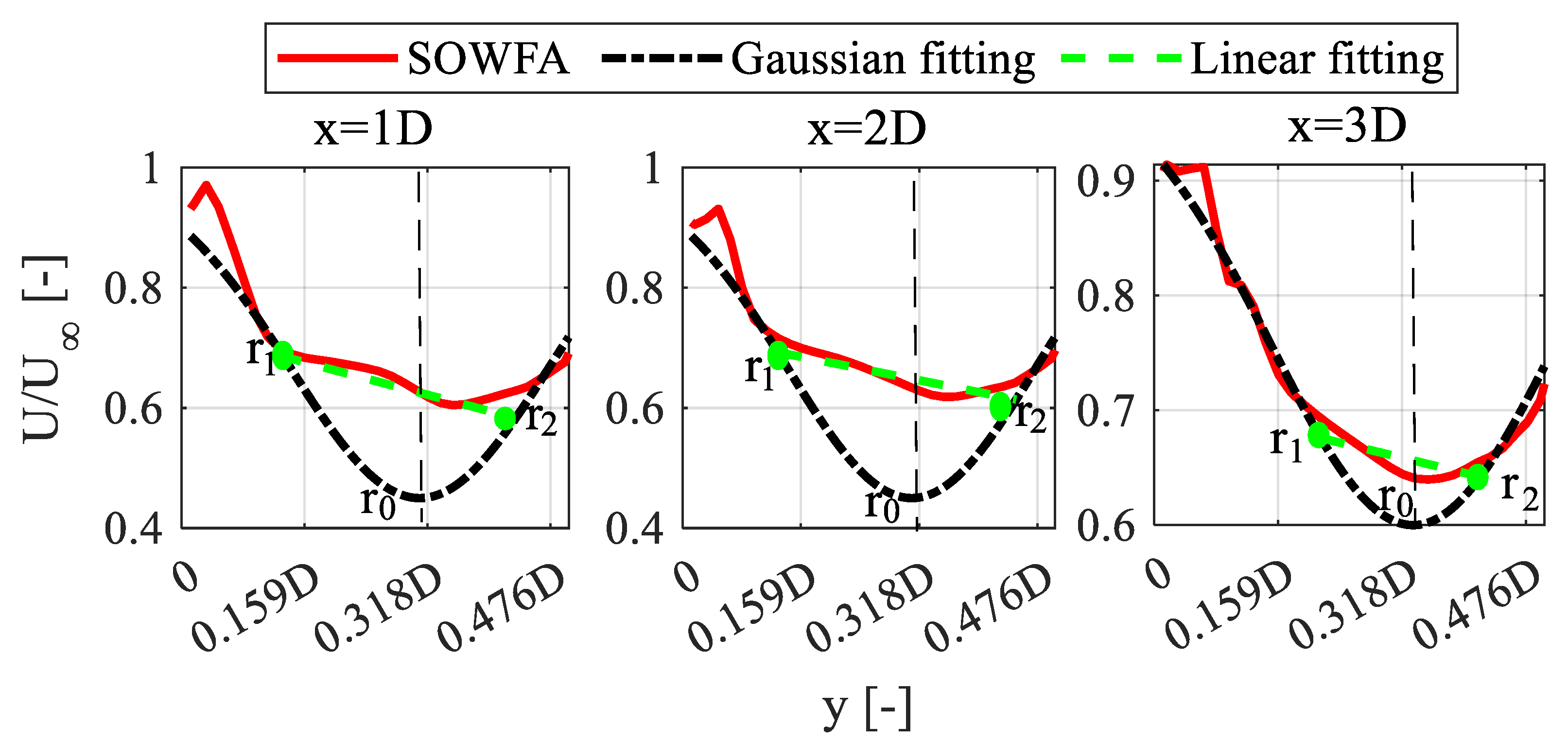
2.2. The Near-Wake Region

With increasing downwind distance, the wake gradually expands under the influence of atmospheric turbulence, and the influence of the blade on the wake profile diminishes. Figure 3 illustrates the rotor’s single-sided radial wake velocity distribution at distances of x = 1D, 2D, and 3D (as shown in Figure 1) simulated using SOWFA. Combining this with Figure 2 on the right, it is observed that, including the initial position, at x = 1D and 2D, the wake loss profiles conform to the piecewise function characteristics. However, at x = 3D, the piecewise function characteristics weaken, and a distinct Gaussian function feature becomes more apparent, where the radial position of Gaussian function extremum defined as $r_0$. Based on this analysis, a reevaluation and modification of the DG wake model will be undertaken in this study.

2.3. Parameter Determination

In accordance with the findings in Section 2.1, due to the expansion of the wake, within the downwind distance of x < 3D, the wake profile exhibits piecewise function characteristics. We hypothesize that the location where the piecewise function characteristics of the wake profile vanish is the flow tube outlet [20], denoted as $x_0$. $x_0$ varies with different wake expansion. Inside the stream tube outlet, where the fluid expansion coefficient is small, the piecewise characteristics of the wake profile are pronounced. On the exterior of the flow tube outlet, where the fluid expansion coefficient is large, the wake profile diffuses into Gaussian features. Hence, in this study, the determination of parameters is divided into two cases: x $\le x_0$ and x $>x_0$. Based on the distribution characteristics of the initial wake deficit distributions in Figure 2, $0.21D/2$ and $0.75D/2$ are identified as the breakpoints for the piecewise function of initial wake deficit distributions. These breakpoints are defined as $r_1$ and $r_2$, respectively, assuming their variations are linear and eventually equal to $r_0$, represented by the following formulas:

$$\mathrm{In} \mathrm{the} \mathrm{horizontal} \mathrm{direction}: \{\begin{array}{c}{r}_1=\frac{0.75D}{2}-\frac{0.21D}{2}{\left(\frac{x}{x_0}\right)}^2\\ r_2=\frac{0.21D}{2}+\frac{x}{x_0}\left(\frac{0.54D}{2}-\frac{0.21D}{2}\frac{x}{x_0}\right)\end{array}$$

(1a)

$$\mathrm{In} \mathrm{the} \mathrm{vertical} \mathrm{direction}: \{\begin{array}{c}{r}_1=\frac{0.75D}{2}-\frac{0.35D}{2}{\left(\frac{x}{x_0}\right)}^2\\ r_2=\frac{0.21D}{2}+\frac{x}{x_0}\left(\frac{0.54}{2}-\frac{0.35D}{2}\frac{x}{x_0}\right)\end{array}$$

(1b)

The breakpoints are dependent on both the stream tube outlet $x_0$ and the downstream distance $x$. The parameter $x_0$ determines the wake expansion function $\sigma \left(x\right)$, which is commonly presumed to vary linearly with the downwind distance $x$. The wake expansion is influenced by the wake recovery and expansion, as illustrated in Equation (2) [20].

$$\sigma \left(x\right)=k_w\left(x-x_0\right)+\epsilon$$

(2)

where $k_w$ is the wake expansion coefficient, ε is the wake expansion at $x_0$. The turbulence intensity $I_w$ is related to the wake expansion factor $k_w$ as follows [23]:

$$\{\begin{array}{c}{I}_w={\left(\frac{0.4C_T{D}^{0.5}}{x^{0.5}}+I_0^{0.5}\right)}^2\\ k_w=k\frac{I_w}{I_0}=k{\left(\frac{0.4C_T{D}^{0.5}}{x^{0.5}{I}_0^{0.5}}+1\right)}^2\end{array}$$

(3)

where $I_0$ is the ambient turbulence intensity, $I_w$ is the wake turbulence intensity, $C_T$ is the thrust coefficient, and $k$ is an identification parameter with different values inside and outside the stream tube outlet $x_0$. Based on high-fidelity simulation results, the location where the wake expansion coefficient exceeds a certain threshold is considered as the stream tube outlet $x_0$. In this study, guided by high-fidelity simulation identification, the expansion coefficient $k_w$ at the flow tube outlet is determined to be 0.0102, then we obtain the following formula,

$$x_0=\frac{{\left(0.4C_T\right)}^{2}D}{{\left(\sqrt{\frac{0.0102}{k}}-1\right)}^2{I}_0}$$

(4)

Moreover, due to the influence of the ground, the evolution of the wake differs in the vertical and horizontal directions. As identified from high-fidelity simulation results:

In the horizontal direction: for $x\le x_0$, $k=0.0037$; $x>x_0$, $k=0.01$;

In the vertical direction: for $x\le x_0$, $k=0.0037$; $x>x_0$, $k=0.015$.

The variation of the Gaussian function’s extreme point $r_0$ is associated with whether it is located within the flow tube outlet. Inside the flow tube outlet, the extreme point exhibits a linear change, while outside the flow tube outlet, the variation is small; in this study, it is assumed to remain constant:

$$\mathrm{In} \mathrm{the} \mathrm{horizontal} \mathrm{direction}: \{\begin{array}{c}{r}_0=\frac{0.63D}{2}-\frac{x}{2x_0}\left(\frac{0.63D}{2}-\frac{0.54D}{2}\right), x\le x_0\\ r_0=\frac{0.54D}{2}, x>x_0\end{array}$$

(5)

$$\mathrm{In} \mathrm{the} \mathrm{vertical} \mathrm{direction}: \{\begin{array}{c}{r}_0=\frac{0.63D}{2}-\frac{x}{2x_0}\left(\frac{0.61D}{2}-\frac{0.4D}{2}\right), x\le x_0\\ r_0=\frac{0.4D}{2}, x>x_0\end{array}$$

(6)

3. Optimized-DG Model

This section incorporates corrections based on blade lift and wake wind speed to adjust the DG wake model. This study refers to this modified model as “Optimized-DG”.

3.1. Derivation of Optimized-DG Model

The general form of the normalized wake model is typically as follows,

$${\widehat{u}}_d=\frac{U_{\infty }-U\left(x,r\right)}{U_{\infty }}=C\left(x\right)f_d\left(D_{\pm }\left(r,x\right),r\right)$$

(7)

where $U_{\infty }$ is the freestream wind speed, $U\left(x,r\right)$ is the wind speed at the radial position $r$ in the wake region at the downwind distance $x$, $C\left(x\right)$ is the wind speed where wake deficit is maximum, and $f_d\left(D_{\pm }\left(r,x\right),r\right)$ is the wake profile.

Assuming that the wake profile conforms to a piecewise function, it is represented as follows:

$$f_d\left(D_{\pm }\left(r,x\right),r\right)=\{\begin{array}{c}{g}_d\left(r,x\right), (r_1\ge r||r\ge r_2)\\ a_1\left(r-r_1\right)+a_2, (r_1<r<r_2)\end{array}$$

(8)

where $g_d\left(r,x\right)$ is a DG function and $a_1\left(r-r_1\right)+a_2$ is the straight line between the breakpoints (in Figure 2 and Figure 3).

$$g_d\left(r,x\right)=\frac{1}{2}\left(e^{D_{+}}+e^{D_{-}}\right), D_{\pm }=-{\left(r\pm r_0\right)}^2/2{\sigma }^2$$

(9)

The parameters $a_1$ and $a_2$ are represented as follows:

$$\{\begin{array}{c}{a}_1=\frac{e^{D_{+}\left(r=r_2\right)}+e^{D_{-}\left(r=r_2\right)}-e^{D_{+}\left(r=r_1\right)}-e^{D_{-}\left(r=r_1\right)}}{2\left(r_2-r_1\right)}\\ a_2=\frac{1}{2}\left(e^{D_{+}\left(r=r_1\right)}+e^{D_{-}\left(r=r_1\right)}\right)\end{array}$$

(10)

Neglecting the viscosity and pressure terms in the momentum equation, based on the principle of momentum conservation, the rate of change of momentum through the rotor disk wind, equivalent to the effective thrust T acting on the rotor disk, is thus expressed as follows:

$$C\left(x\right)=\frac{M\pm \sqrt{M^2-\frac{1}{2}N{C}_T{d}_0^2}}{2N}\left(e^{D_{+}}+e^{D_{-}}\right)$$

(11)

where,

$$M={\displaystyle \int }r\left(f_d\left(D_{\pm }\left(r,x\right),r\right)\right)dr$$

(12a)

$$N={\displaystyle \int }r{\left(f_d\left(D_{\pm }\left(r,x\right),r\right)\right)}^{2}dr$$

(12b)

for $x\le x_0$, derived from (12a) and (12b),

$$M_n=2{\sigma }^2{e}^{\frac{-r_0^2}{2{\sigma }^2}}+\sqrt{2\pi }{r}_0\sigma erf\left(\frac{r_0}{\sqrt{2}\sigma }\right)+a_1\left(\frac{r_2^3}{3}-\frac{r_1{r}_2^2}{2}-\frac{r_1^3}{6}\right)+a_2\left(r_2^2-r_1^2\right)$$

(13a)

$$\begin{gathered} N_n=\frac{1}{2}(a_1^2\left(\frac{1}{4}{r}_2^4-\frac{2}{3}{r}_2^3{r}_1+\frac{1}{2}{r}_1^2{r}_2-\frac{1}{4}{r}_1^4+\frac{1}{6}{r}_1^3\right)+2a_1{a}_2\left(\frac{1}{3}{r}_2^3+\frac{1}{6}{r}_1^3-\frac{1}{2}{r}_2^2{r}_1\right) \\ \hspace{0.17em}\hspace{0.17em}\hspace{0.17em}\hspace{0.17em}\hspace{0.17em}\hspace{0.17em}\hspace{0.17em}\hspace{0.17em}\hspace{0.17em}\hspace{0.17em}\hspace{0.17em}\hspace{0.17em}\hspace{0.17em}\hspace{0.17em}\hspace{0.17em}\hspace{0.17em}\hspace{0.17em}\hspace{0.17em}\hspace{0.17em}\hspace{0.17em}\hspace{0.17em}\hspace{0.17em}\hspace{0.17em}\hspace{0.17em}\hspace{0.17em}\hspace{0.17em}\hspace{0.17em}\hspace{0.17em}\hspace{0.17em}+\frac{1}{2}{a}_1^2\left(r_2^2-r_1^2\right)+2{\sigma }^2{e}^{\frac{-r_0^2}{{\sigma }^2}}+{\sigma }^2\left(e^{-\frac{r_2^2+r_0^2}{{\sigma }^2}}-e^{-\frac{r_1^2+r_0^2}{{\sigma }^2}}\right)+\sqrt{\pi }\sigma erf\left(\frac{r_0}{\sigma }\right) \\ \hspace{0.17em}\hspace{0.17em}\hspace{0.17em}\hspace{0.17em}\hspace{0.17em}\hspace{0.17em}\hspace{0.17em}\hspace{0.17em}\hspace{0.17em}\hspace{0.17em}\hspace{0.17em}\hspace{0.17em}\hspace{0.17em}-\frac{{\sigma }^2}{2}\left(e^{\frac{-{\left(r_1+r_0\right)}^2}{{\sigma }^2}}+e^{\frac{-{\left(r_1-r_0\right)}^2}{{\sigma }^2}}-e^{\frac{-{\left(r_2+r_0\right)}^2}{{\sigma }^2}}+e^{\frac{-{\left(r_2-r_0\right)}^2}{{\sigma }^2}}\right) \\ \hspace{0.17em}\hspace{0.17em}\hspace{0.17em}\hspace{0.17em}\hspace{0.17em}\hspace{0.17em}\hspace{0.17em}\hspace{0.17em}\hspace{0.17em}\hspace{0.17em}\hspace{0.17em}\hspace{0.17em}\hspace{0.17em}\hspace{0.17em}\hspace{0.17em}-\frac{\sqrt{\pi }}{2}{r}_0\sigma (erf\left(\frac{r_1+r_0}{\sigma }\right)-erf\left(\frac{r_1+r_0}{\sigma }\right)-erf\left(\frac{r_2+r_0}{\sigma }\right) \\ +erf\left(\frac{r_2-r_0}{\sigma }\right))\hspace{0.17em}\hspace{0.17em}\hspace{0.17em}\hspace{0.17em}\hspace{0.17em}\hspace{0.17em}\hspace{0.17em}\hspace{0.17em}\hspace{0.17em}\hspace{0.17em}\hspace{0.17em}\hspace{0.17em}\hspace{0.17em}\hspace{0.17em}\hspace{0.17em}\hspace{0.17em}\hspace{0.17em}\hspace{0.17em}\hspace{0.17em}\hspace{0.17em}\hspace{0.17em}\hspace{0.17em}\hspace{0.17em}\hspace{0.17em}\hspace{0.17em}\hspace{0.17em}\hspace{0.17em}\hspace{0.17em}\hspace{0.17em}\hspace{0.17em} \end{gathered}$$

(13b)

With the expansion of the wake, the influence of the blades on the wake gradually becomes less pronounced. Eventually, at the outlet of the flow tube, $r_1$ and $r_2$ converge to the same location, and the piecewise function characteristics disappear, for $x\le x_0$, yielding,

$$M_f=2{\sigma }^2{e}^{\frac{-r_0^2}{2{\sigma }^2}}+\sqrt{2\pi }{r}_0\sigma erf\left(\frac{r_0}{\sqrt{2}\sigma }\right)$$

(14a)

$$N_f={\sigma }^2{e}^{\frac{-r_0^2}{{\sigma }^2}}+\frac{\sqrt{\pi }}{2}{r}_0\sigma erf\left(\frac{r_0}{\sigma }\right)$$

(14b)

Derived from the above formulas: in the wake region where $x\le x_0$, the expression for the wake loss function is as follows:

$${\widehat{u}}_d=\{\begin{array}{c}\frac{M_n-\sqrt{M_n^2-\frac{1}{2}{N}_n{C}_T{D}^2}}{2N_n}{g}_d\left(r,x\right), (r_1\ge r||r\ge r_2)\\ \frac{M_n-\sqrt{M_n^2-\frac{1}{2}{N}_n{C}_T{D}^2}}{2N_n}\left(a_1\left(r-r_1\right)+a_2\right), (r_1<r<r_2)\end{array}$$

(15)

In the wake region where $x>x_0$, the expression for the wake loss function is as follows:

$${\widehat{u}}_d=\frac{M_f-\sqrt{M_f^2-\frac{1}{2}{N}_f{C}_T{D}^2}}{2N_f}{g}_d\left(r,x\right)$$

(16)

3.2. Considering the Optimized-DG Model with Wind Shear

Vertical wind shear is a common atmospheric boundary layer effect, leading to an uneven distribution of wind speed in the vertical direction. It is crucial to consider this effect in wake calculations. In this study, an exponential model of wind shear is employed.

$$U\left(z\right)=U_{hub}{\left(\frac{z+z_h}{z_h}\right)}^{\alpha }$$

(17)

where $z_h$ is the height of the hub center, $z$ is the vertical height with $z_h$ as the reference position, $U_{hub}$ is the wind speed at the hub center, and $\alpha$ is the wind shear exponent. The three-dimensional wake loss wind speed is expressed as follows:

$$u_d\left(x,y,z\right)=\{\begin{array}{c}{C}_n\left(x\right)f_d\left(D_{\pm }\left(y,z,x\right),r\right), \left(x\le x_0\right)\\ C_f\left(x\right)f_d\left(D_{\pm }\left(y,z,x\right),r\right), (x>x_0)\end{array}$$

(18)

where $r=\sqrt{y^2+{\left(z-z_h\right)}^2}$

$$C_n\left(x\right)=\frac{M_n-\sqrt{M_n^2-\frac{1}{2}{N}_n{C}_T{D}^2}}{2N_n}, C_f\left(x\right)=\frac{M_f-\sqrt{M_f^2-\frac{1}{2}{N}_f{C}_T{D}^2}}{2N_f}$$

(19)

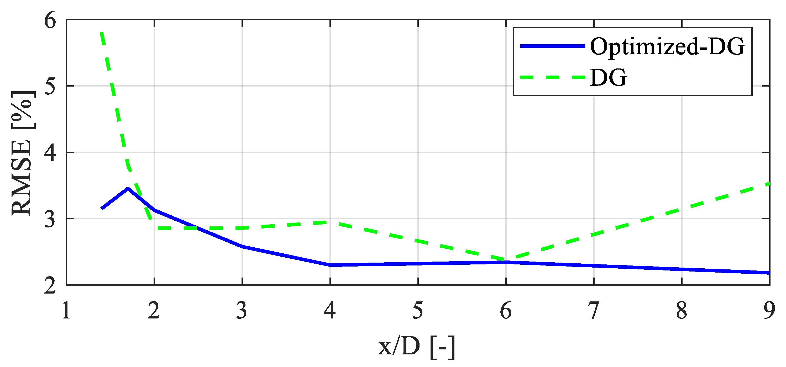
3.3. Validation of the Optimized-DG Model

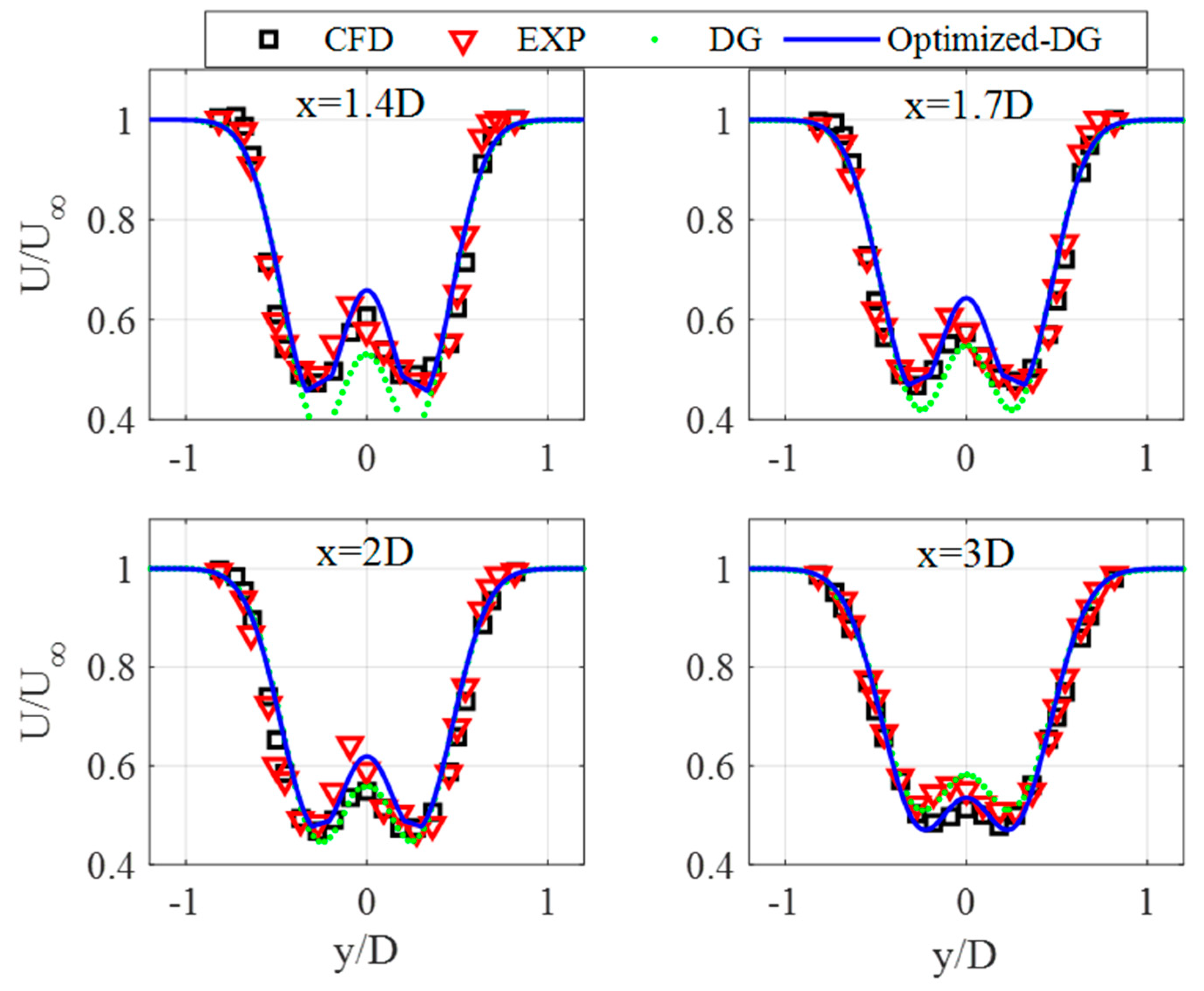
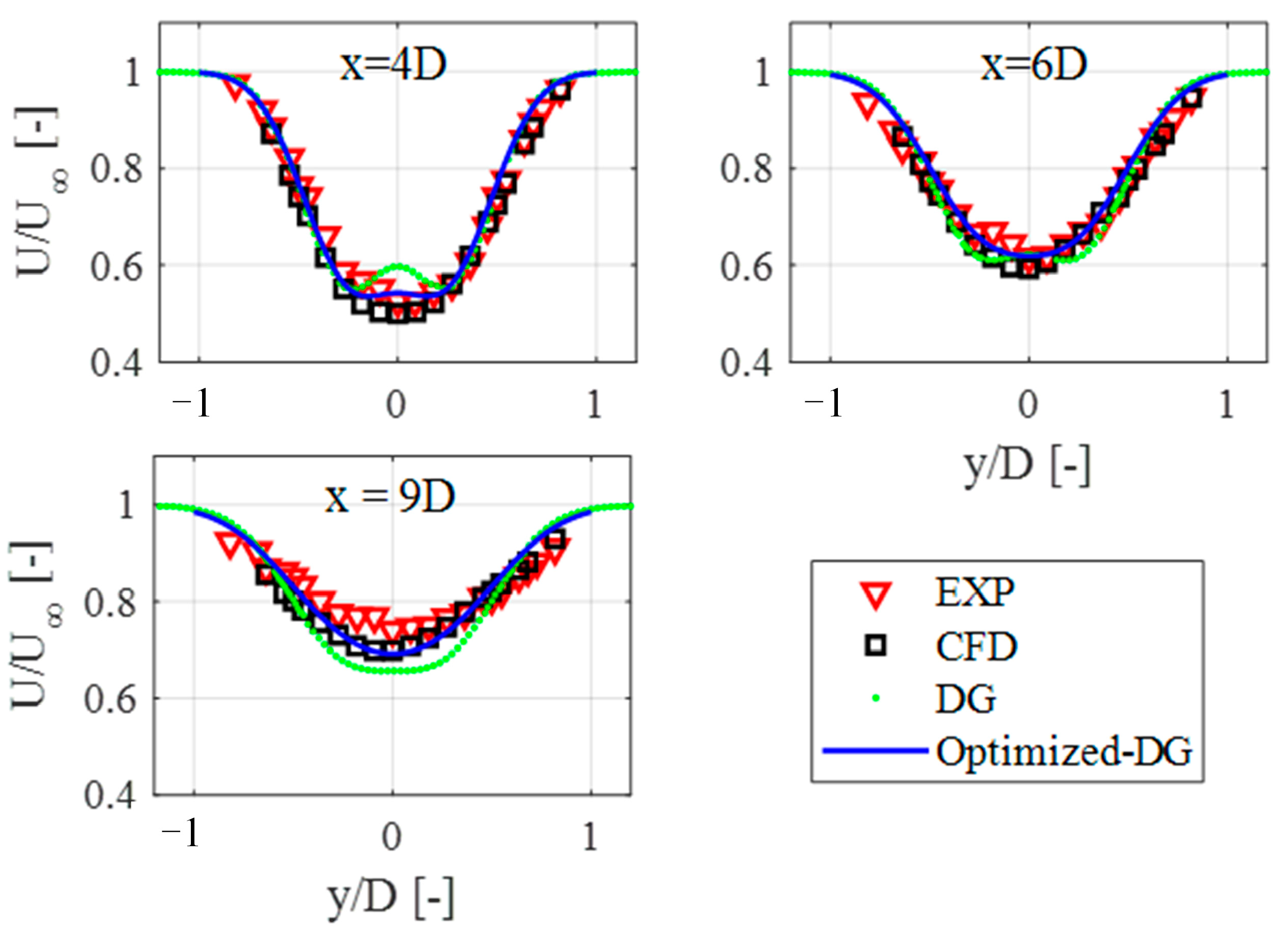
3.3.1. Validation of Horizontal Profile

This part utilizes wake measurement data and simulation data from existing literature [20]. The physical model of the turbine has a rotor diameter of 1.1 m and a hub height of 0.8 m, which are proportionally scaled to the NREL 5 MW Baseline wind turbine with a diameter of 126 m and a hub height of 90 m. The data in reference [20] can be used as a reference, giving a thrust coefficient of 0.75, a wind speed of 5 m/s, and a turbulence intensity of 6%.

Figure 4 provides a comparative analysis of horizontal wake velocity profiles at four downstream near-wake locations ($x=1.4D, 1.7D, 2D, 3D$) at the hub height. Experimental data (EXP), CFD data, and the wake model data from DG are compared with the Optimized-DG model. The horizontal axis represents the nondimensional distance from the rotor plane in the horizontal direction to the hub center, normalized by the wind rotor diameter. The vertical axis represents the nondimensional wake velocity compared to the velocity at the hub center.

Examining the wake loss profiles from EXP and CFD, the DG features are notably evident within the $x\le 3D$ range. Both the DG and Optimized-DG models effectively capture these features with high precision, particularly near the extremum points for Optimized-DG. However, at $x=1.4D$ and $x=1.7D$, where the impact of the blades on the wake is significant, DG exaggerates the wake loss near the extremum points. The wake profile described by Optimized-DG accurately represents the characteristics near the extremum points, significantly enhancing the precision of the wake. In the vicinity of $y=0$, especially at $x=2D$, the Optimized-DG model estimates wind speeds lower than CFD and EXP values. This discrepancy may be attributed to an overestimation of the Gaussian extremum point. Nevertheless, the Optimized-DG model demonstrates a high level of agreement with CFD experimental data at $x=3D$, indicating its capability to effectively handle the transition in wind speed calculations at the flow tube outlet position.

Figure 5 illustrates the wake distribution at three horizontal planes ($x=4D, 6D, 90; z=9D$) in the downstream far-wake region. At $x=4D$ and $x=6D$, both EXP and CFD data exhibit good agreement with the Optimized-DG model. In particular, at the transition from DG to Gaussian characteristics in the wake, the Optimized-DG model provides a more accurate estimate compared to the DG model. This enhancement is attributed to the correction of the Gaussian extremum point, which more precisely captures the evolution of the average wake profile. At $x=9D$, the DG model overestimates the wake loss, while the Optimized-DG model optimizes this estimation, indicating that the corrected wake spreading function in the Optimized-DG model is more accurate. In summary, the corrected spreading function and Gaussian extremum point demonstrate effective wake loss corrections at $x=4D, 6D$, and $9D$.

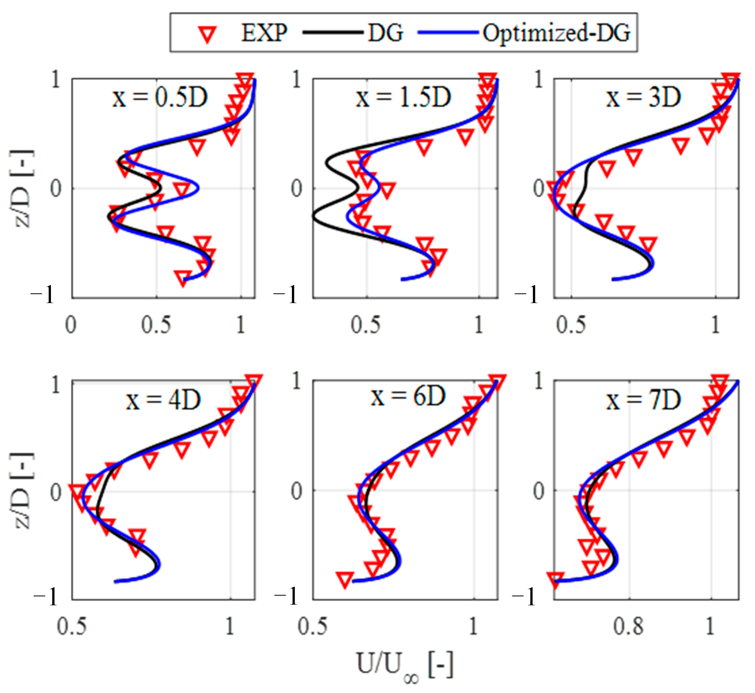
3.3.2. Validation of Vertical Profile

To validate the accuracy of the wind shear-considering model estimates, we reference the wake data measured using lidar in the existing literature [16]. The measured wind turbine has a hub height of 65 m, a rotor diameter of 77 m, a hub center wind speed of 9.2 m/s, a turbulence intensity of 11% over ten minutes, and a thrust coefficient of 0.72; the fitted wind shear exponent is 0.14.

Figure 6 illustrates the comparison results between the wake model estimates and the wake measurement data on six vertical profiles. The horizontal axis represents the vertical wake velocity normalized by the inflow velocity at the hub center, while the vertical axis represents the height normalized by the rotor diameter, with the hub center height as the reference. The Optimized-DG model clearly exhibits wind shear characteristics, aligning well with the measured data. At positions close to the wind turbine (x = 0.5D, x = 1.5D, x = 3D), the Optimized-DG model significantly outperforms the DG model when compared to experimental data. However, due to the tilt of the wind turbine rotor, causing the two break-points in the vertical direction to be relatively close, they prematurely overlap during the evolution of the wake. Therefore, no distinct segmentation features are observed in the vertical direction.

Additionally, as shown in Figure 6, in the wake region where $x \le 3D$ and in the vertical zone where z > 0.5D, the Optimized-DG model overestimates the wake velocity. This phenomenon may originate from contingency in the measured wind speed, which does not exactly fit the fitted wind shear model. Therefore, the Optimized-DG model tends to overestimate the vertical velocity in this region. At $x=3D$, the Optimized-DG model overestimates the wake radius compared to the measurement. This error could be attributed to the Optimized-DG model overestimating the wake expansion coefficient under high turbulence intensity, exaggerating the vertical expansion of the wake (neglecting the inhibiting effect of the ground on wake expansion). In the zone $x=6, 7D$, $z<-0.5D$, the Optimized-DG model consistently overestimates the wake velocity. This discrepancy may arise from the influence of ground roughness on wake diffusion, an effect not accounted for in the Optimized-DG model. Therefore, the Optimized-DG model does not align with the wind speed measurements close to the ground.

To compare the accuracy between the optimized DG model and the DG model with CFD data as the reference, the root mean square error (RMSE) is calculated separately. This is shown in Figure 7, where, compared to the DG model, the Optimized-DG model demonstrates an overall lower RMSE. Consistent with the observations in Figure 6 and Figure 7, at $x=1.4D$ and $1.7D$, the Optimized-DG wake model significantly reduces the RMSE values. At $x=2D$, the Optimized-DG model exhibits a slightly higher RMSE compared to the DG model. However, at positions ranging from $x=3D \mathrm{to} x=9D$, the RMSE is consistently lower for the Optimized-DG model compared to the DG model. This indicates an overall higher estimation accuracy of the wake model, with significant improvement in estimation precision for the Optimized-DG model compared to the DG model.

4. Wind Turbine Load and Power Estimation Based on the Optimized-DG Model

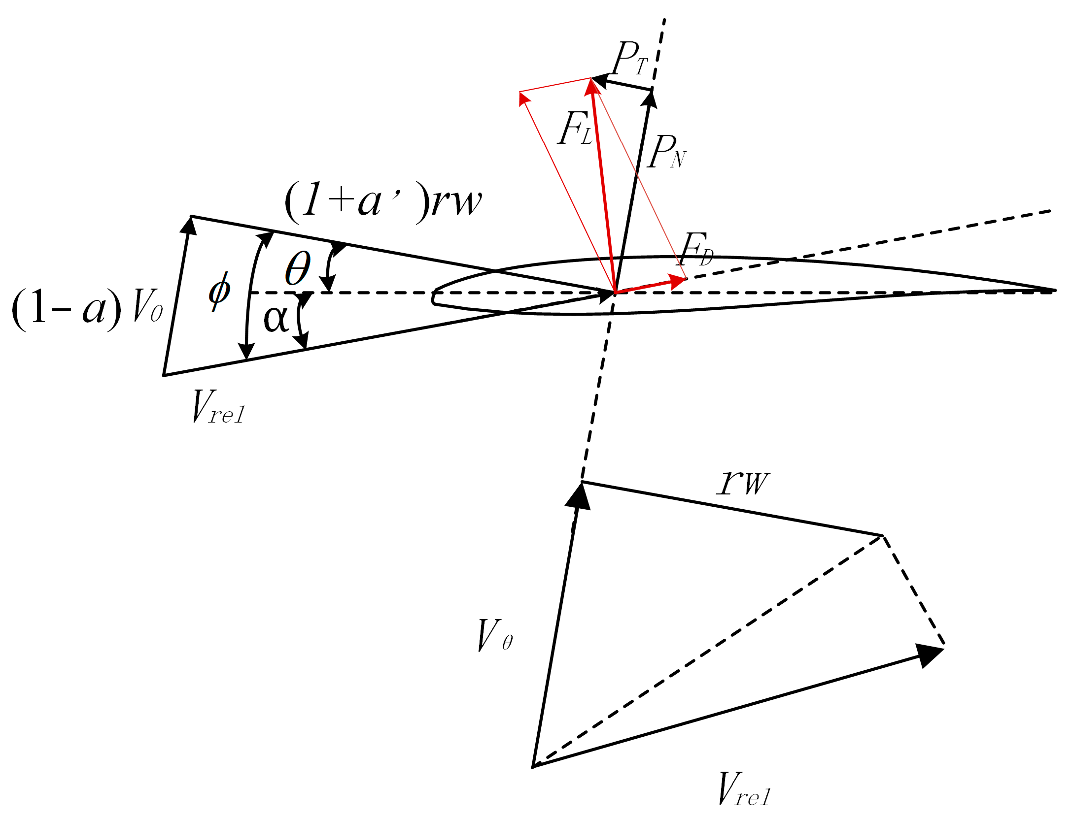
4.1. Development and Validation of Blade Root Flap-Wise Moments and Power

In accordance with the principles of the Blade Element Momentum(BEM) theory [24], shown in Figure 8, the lift and drag forces experienced by the blade element can be delineated as follows:

$$\{\begin{array}{c}d{F}_L=\frac{1}{2}\rho V_{rel}^{2}c{C}_{l}dr\\ d{F}_D=\frac{1}{2}\rho V_{rel}^{2}c{C}_{d}dr\end{array}$$

(20)

where $\rho$ represents air density, $V_{rel}$ represents the relative wind speed, $c$ represents the airfoil chord length at the blade element, $C_l$ represents the lift coefficient, and $C_d$ represents the drag coefficient.

The axial and tangential forces generated on the blades by the blade elements are obtained from the conversion of lift and drag, as given in Formula (20). The axial and tangential forces of each blade element can be determined by the following matrix transformation:

$$\{\begin{array}{l}{P}_N=F_L\cos \varphi +F_D\sin \varphi \hfill \\ P_T=F_L\sin \varphi -F_D\cos \varphi \hfill \end{array}$$

(21)

where $\varphi$ is inflow angle of the $\mathrm{i} \mathrm{th}$ blade, $P_N$ is the blade root flap-wise moment, $P_T$ is the blade root edge-wise moment.

According to (21), the blade root flapping load is determined by local wind speed, rotor speed, thrust coefficient, drag coefficient, and inflow angle. The BEM solver from AeroDyn [25] can be used to obtain $C_l$, $C_d$, and inflow angle $\varphi$ under the corresponding working conditions, and then obtain $P_N$ according to (21). Due to the close correlation between blade root flap-wise loads and wind speed, the above-mentioned method utilizes the Optimized-DG model to calculate the blade root flap-wise loads by obtaining the wind speed distribution within the rotor plane. However, in practice, the blade root flap-wise loads of offshore floating wind turbines are simultaneously influenced by both waves and wind conditions. Therefore, in this scenario, a nonlinear model is proposed based on FAST’s rapid calculations, fitted with hundreds of thousands of simulated conditions, taking into consideration the impact of waves on blade root flap-wise moment,

$$M_{yi}=\mathit{A}\times {\left[v_i, \omega , {\beta }_i, {\psi }_i, W,v_i\omega , v_i{\beta }_i,v_i{\psi }_i, v_i W, \omega {\beta }_i, \omega {\psi }_i,\omega W, {\beta }_i{\psi }_i, {\beta }_{i}W, {\psi }_{i}W, v_i^2, {\omega }^2, {\beta }_i^2, {\psi }_i^2, W^2\right]}^T$$

(22)

where $v_i$ is the local wind speed, $\omega$ is the rotor speed, ${\beta }_i$ is the pitch angle, ${\phi }_i$ is the azimuth angle, and $W$ is the average wave height. $\mathit{A}$ are the coefficient matrix of the nonlinear model. According to the blade element theory, the power generated by the blade element is expressed as follows:

$$P={\displaystyle \int }\frac{1}{2}\rho v^3{C}_{p}d{A}_d, d{A}_d=2\pi rdr$$

(23)

The BEM solver from AeroDyn [25] was also used to obtain $C_p$, and then to obtain the power. Due to the action of waves, the relative motion of the wind turbine will alter the relative wind speed. Therefore, similarly using the method of fitting blade root flap-wise loads, determining the power of the wind turbine involves recognizing it as a nonlinear function related to wind speed, rotor speed, pitch angle, and wave.

$$P=\mathit{B}\times {\left[v_i, \omega , {\beta }_i, {\psi }_i, W,v_i\omega , v_i{\beta }_i,v_i{\psi }_i, v_i W, \omega {\beta }_i, \omega {\psi }_i,\omega W, {\beta }_i{\psi }_i, {\beta }_{i}W, {\psi }_{i}W, v_i^2, {\omega }^2, {\beta }_i^2, {\psi }_i^2, W^2\right]}^T$$

(24)

where $\mathit{B}$ are the coefficients matrix of the nonlinear model. To validate the accuracy of the model (22) and (24), the nonlinear model fitted for a semi-submersible floating wind turbine is compared with the OpenFAST [26] result. In this section, the simulation conditions are set at a wind speed of 12 m/s, turbulence intensity of 6%, and wind shear of 0.13, as shown in Figure 9 (top). Waves are generated by regular and irregular incident wave kinematics models; the significant wave height of incident waves of the two models are 2 m, as shown in Figure 9 (bottom), where the vertical axis represents wave height. Two sets of simulations were established to investigate the impact of waves on model estimates, as shown in

Table 1. Sea conditions settings.

Experiments	Sea Conditions
Test 1	Regular waves
Test 2	Irregular waves

.

Estimated blade-root flap-wise loads (${\mathrm{M}}_{\mathrm{y}1}$) and power are obtained through simulations, as depicted in Figure 10. The horizontal axis is represented by time, while the vertical axis corresponds to normalized variables. Upon scrutinizing the OpenFAST results of ${\mathrm{M}}_{\mathrm{y}1}$ (first and second rows) and power (third and fourth rows), it becomes apparent that despite minor variations in variables across distinct sea conditions, noteworthy observations can still be made. Comparative analysis with OpenFAST outcomes reveals that the nonlinear model adeptly captures the evolving trends in ${\mathrm{M}}_{\mathrm{y}1}$ and power. The precision in calculating ${\mathrm{M}}_{\mathrm{y}1}$ is substantial, whereas the accuracy in power estimation is comparatively lower. The extant error is, in part, attributed to variables not accounted for within the nonlinear model and, alternatively, may arise due to the model overlooking dynamic responses. Through comprehensive computations of average values derived from FAST and the nonlinear model, it is discerned that the disparity between them is exceedingly marginal. This underscores the capability of the nonlinear model to represent the mean behavior of the wind turbine amid wake disturbances.

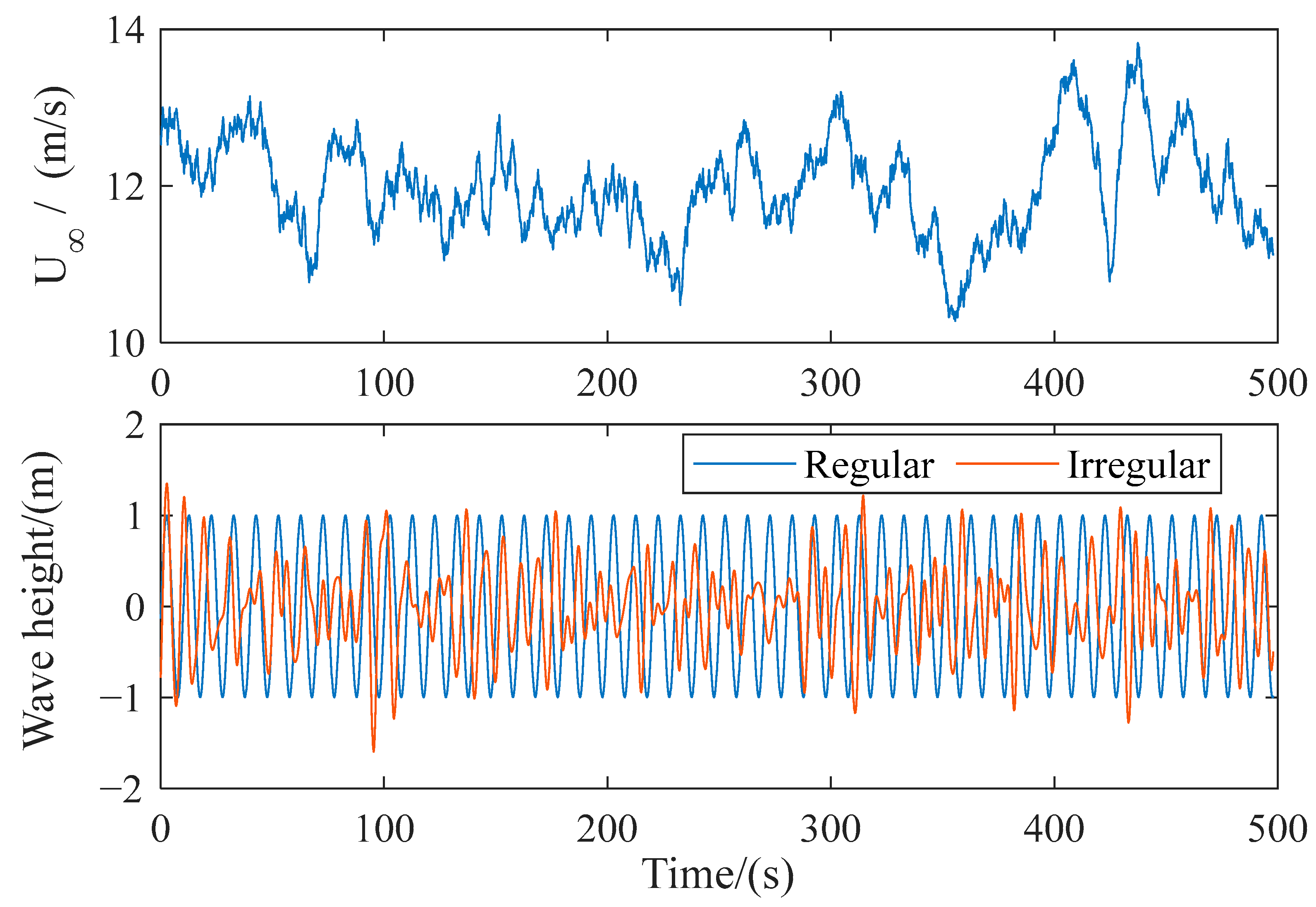
4.2. Simulation Settings and Wind Speed Acquisition for Load and Power Estimation

To apply the Optimized-DG model to the estimation of load effects caused by wake interference, it is necessary to obtain the wind speed distribution on the rotor plane. High-fidelity simulations of the NREL 5 MW wind turbine were conducted using SOWFA; wind field parameters are shown in

Table 2. Wind field parameters for NREL 5 MW wind turbine.

Description	Unit	Value
Rated power	MW	5
Rotor diameter/hub diameter	m	126/3
Cut-in/Rated/cut-out wind speed	m/s	3/11.4/25
Hub Center Wind Speed	m/s	12
Atmospheric Turbulence Intensity		6%
Wind shear		0.13
Thrust Coefficient ($C_T$)		0.72

and configuration information for SOWFA is in

Table 3. Configuration information for SOWFA.

Description	Unit	Value
Horizontal Spatial Dimensions of the Turbine	m2	500 × 500
Simulation Space Size	km3	2.5 × 1.25 × 1.25
Simulation Grid Division		800 × 400 × 400
Simulation Grid Size of Locally refined region	m	3.125
Time step	s	0.5

.

Since the downstream wind turbine’s position relative to the wake is random, it is necessary to validate the model’s disk wind speed at different downstream distances x and lateral positions y, as illustrated in Figure 1b by the red circles, measuring radius $r=\frac{2}{3}R$ [26].

To compare the results obtained from the specified locations with SOWFA and the Optimized-DG model, wake data were acquired at positions $x=3D, 6D, 9D$; $y=1D, 0.5D, 0D,-0.5D,-1D$.

Assuming the downstream wind turbine position is changed to different downstream locations (x, y) as shown in Figure 1b, the positions selected for verification of wake estimation accuracy at different downstream locations are x = 3D, 6D, 9D and y = 1D, 0.5D, 0, −0.5D, −1D, totaling 15 positions. Figure 11 illustrates the comparison between the Optimized-DG model estimates and wake data profiles in SOWFA. The horizontal axis represents the azimuth angle ($\psi \in [0,360]$ degree) within the rotor plane, and the vertical axis displays normalized estimated wind speeds $U/U_{\infty }$, $U_{\infty }$ is the freestream wind speed at the hub center without wake interference as the reference. The wind speed profiles obtained from SOWFA at various azimuth angles demonstrate that the Optimized-DG model exhibits good estimation accuracy. However, the Optimized-DG model demonstrates symmetry in the wake, as observed at $x=3D, 6D,9D; y=0.5D,-0.5D$. This symmetry is assumed due to the assumed self-symmetry of the wake. In fact, minor variations in the wake caused by rotor rotation, blade deformation, and other factors have not been considered in the optimized-DG model, and these wake changes are very small and thus neglected in this study.

4.3. Rapid Blade Root Flap-Wise Load and Power Estimation Based on Optimized-DG

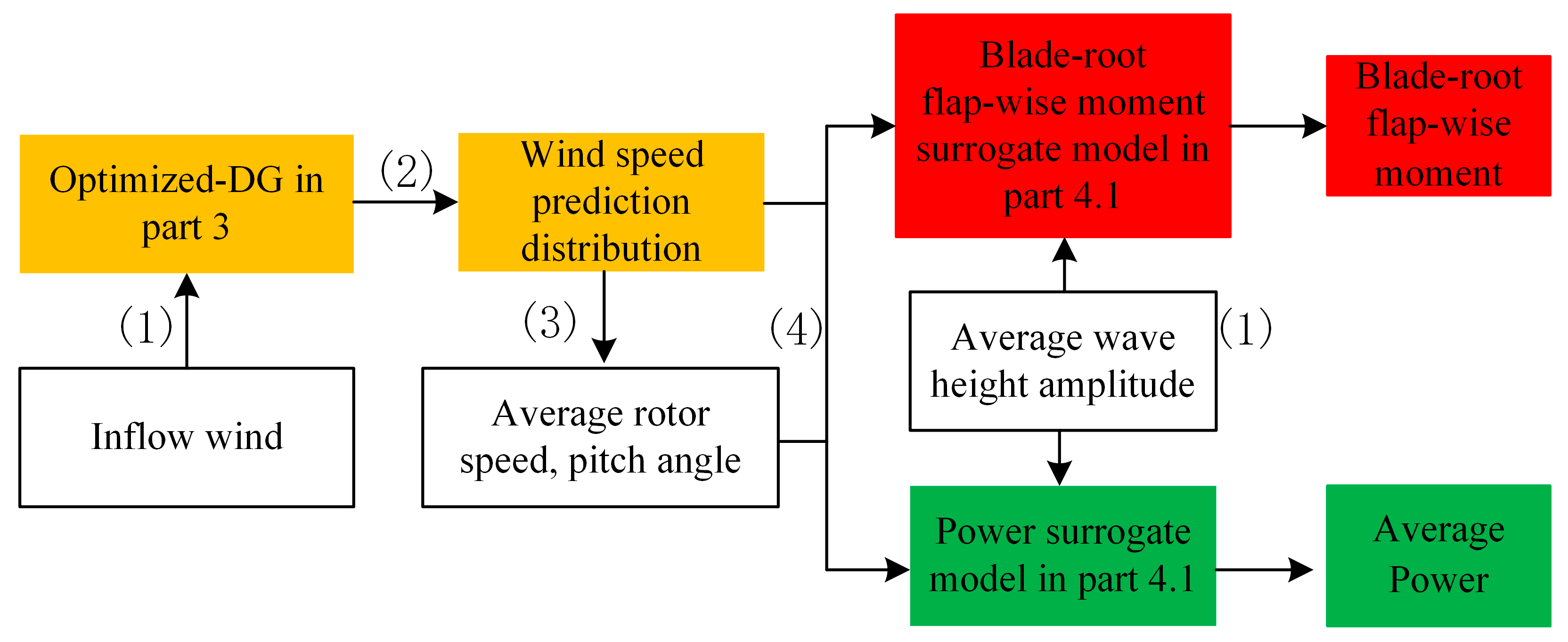
The following steps involve estimating the wake wind speed based on the combined Optimized-DG method to assess the blade-root flap-wise moment and power. The procedure is illustrated in Figure 12 and is executed as follows:

(1)

The inflow wind speed and wave height are obtained from the measured average wind speed and significant wave height at the upwind turbine location.

(2)

Fit a wind shear model based on the measured free-stream wind speed. Combine this with the Optimized-DG model in part 3 to jointly compute the wake wind speed distribution on the rotor plane at downstream positions.

(3)

Calculate the average wind speed on the rotor plane based on the wake wind speed distribution obtained in (2). Utilize the steady-state response of the wind speed function [5 MW] to determine the corresponding average rotor speed and blade pitch angle for the average wake wind speed [27].

(4)

Utilize the proxy model for blade root flap-wise loads and power presented in Section 4.1 to calculate blade root flap-wise loads and power influenced by wake disturbances.

To characterize the roles of different parts in the flowchart, yellow rectangles represent the wake estimation section, red denotes the load estimation section, and green indicates the power estimation section.

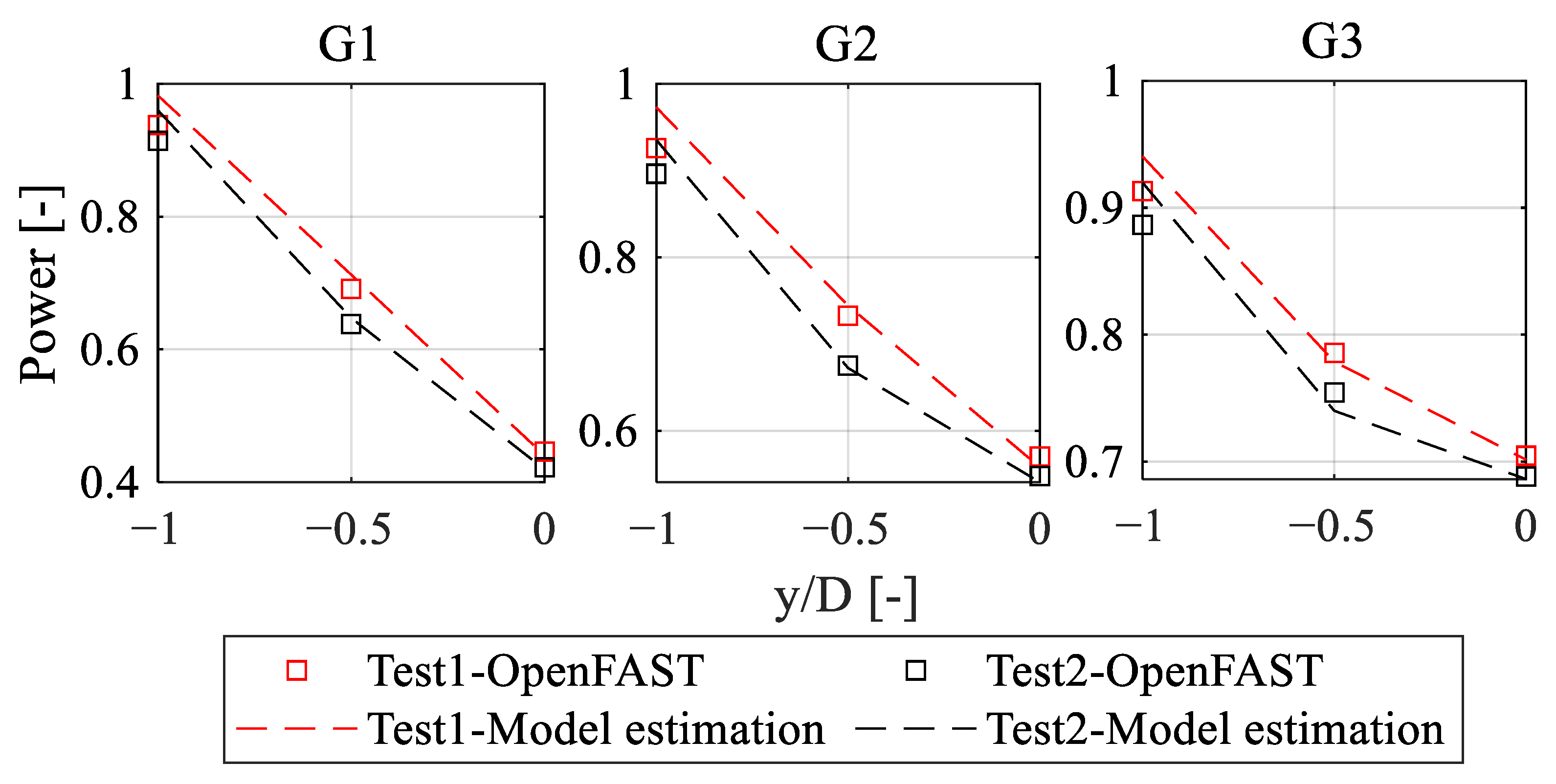
4.4. Simulation Validation

Couple the wake wind speeds simulated in Section 4.1 of SOWFA into OpenFAST. To validate the blade-root flap-wise load estimation based on Optimized-DG, the simulation was conducted under the operational conditions of a semi-submersible floating wind turbine. Due to the symmetry of wind speeds, to simplify the problem, we only investigate wake load and power estimates at y = 0, −0.5D, and −1D positions, and the simulations are designed as in

Table 4. Simulation design.

Group	Test	x	y	Wave Type
G1	Test 1	$x=3D$	0/−0.5D/−1D	regular
	Test 2	$x=3D$	0/−0.5D/−1D	irregular
G2	Test 1	$x=6D$	0/−0.5D/−1D	regular
	Test 2	$x=6D$	0/−0.5D/−1D	irregular
G3	Test 1	$x=9D$	0/−0.5D/−1D	regular
	Test 2	$x=9D$	0/−0.5D/−1D	irregular

.

The primary focus of this study is on the wind speed non-uniformity caused by wake disturbances. Therefore, OpenFAST data was obtained to validate the model estimates of average blade root flap-wise moments at different azimuth angles.

Figure 13, Figure 14 and Figure 15 depict the comparison between the estimated blade-root flap-wise loads ${\mathrm{M}}_{y1}$ in the G1, G2, and G3 simulations and the OpenFAST results. The values of ${\mathrm{M}}_{y1}$ on the vertical axis have been normalized, with the normalization reference being the maximum blade root flap-wise load obtained from the OpenFAST simulations at x = 3D, y = −0.5D, as indicated by the marker in the first row, second column of Figure 13. The blue lines in the figures represent the model estimates, while the red squares indicate the OpenFAST results. Overall, the model estimates align well with the OpenFAST results.

Each row in the figures corresponds to Test1 and Test2, where the x-axis represents the azimuth angle on the rotor plane, and the y-axis represents the normalized blade root flap-wise moments. The blade root flap-wise load reflects the variation trend caused by wake, wind shear, and blade pitch angle within the rotor plane. At different downstream distances, the blade root flap-wise load exhibits the following patterns: smaller average load in the near-wake region and larger average load in the far-wake region. At the y = −0.5D position, the load fluctuation amplitude is maximum, while at y = 0, −1D, the load fluctuation amplitude is smaller.

Validation with OpenFAST results indicates that the model estimates can accurately track the variation of blade root flap-wise loads with azimuth angles within the rotor plane. The model can precisely identify the minimum and maximum load values and their corresponding azimuth angles. However, at y = 0 and y = −1D, OpenFAST results show that, around the azimuth angle of 200 degrees, the load exhibits a different trend from its surroundings, which the model fails to capture. This difference may be attributed to external factors not considered by the model.

For downstream wind turbines, as the wake coverage area increases and the downstream distance decreases, the average blade root flap-wise load decreases. However, the maximum load at y= −1D is smaller than the maximum at y = −0.5D. This is because when the average wind speed in the rotor plane is higher than the rated wind speed, the blade pitch angle is greater than zero, leading to a reduction in blade root flap-wise load. The increase in downstream distance, x, results in an increase in blade root flap-wise load. However, this characteristic is not observed at y = −1D for x = 3D, x = 6D, and x = 9D, as the wake interference is minimal at this position, resulting in small load fluctuations. Although the model’s accuracy is not consistently high at every azimuth angle, it provides a relatively good description of maximum and minimum values.

Additionally, there is minimal difference in accuracy between sine wave and harmonic wave load estimations, indicating the model’s ability to capture such variations.

According to the statistical results mentioned above, the maximum error of the model-estimated blade root flap-wise loads at different azimuth angles is 10.02%, compared to the corresponding OpenFAST results, with an average error of 3.93%. This modeling estimation method demonstrates its practicality in the low-frequency estimation of blade root flap-wise loads influenced by wake disturbances. It provides valuable reference for understanding load fluctuations in wake control strategies implemented within wind farms.

In wake control, there is often little concern about power fluctuations due to changes in azimuth angles, but rather a focus on the average power value. Therefore, unlike the approach used to study blade root flap-wise loads, the average power at different positions is estimated. As shown in Figure 16, the wind turbine exhibits varying power losses at different locations. This indicates that as the downstream distance increases, power loss decreases, and the larger the wake interference area, the greater the power loss. In general, the nonlinear model is capable of estimating power under wake interference. Among all layouts, when y/D = 0, the power estimation demonstrates the highest accuracy, while at y/D = −0.5 and −1, the accuracy of power estimation is relatively lower. This may be attributed to the accuracy of wind estimation, as explained in the wind speed analysis in Section 4.2. Considering all cases, the maximum error in power estimation is 3%, with an average error of 1%.

5. Conclusions

In the previous engineering wake models, the unique characteristics of initial wake velocities right behind the rotor by blades were not considered, adversely impacting the accuracy of wind speed estimates in the near-wake region. To address this issue, this study, based on an analysis of the wake velocity distribution right behind the rotor, proposes varying wake parameters with downstream distance and modifies the DG wake model, introducing the Optimized-DG wake model. Furthermore, an estimation method for the fluctuation of blade-root flap-wise loads under wake interference is proposed based on the wake model. All models are validated through experiments and CFD simulations to ensure their accuracy. The summarized results are as follows:

(1)

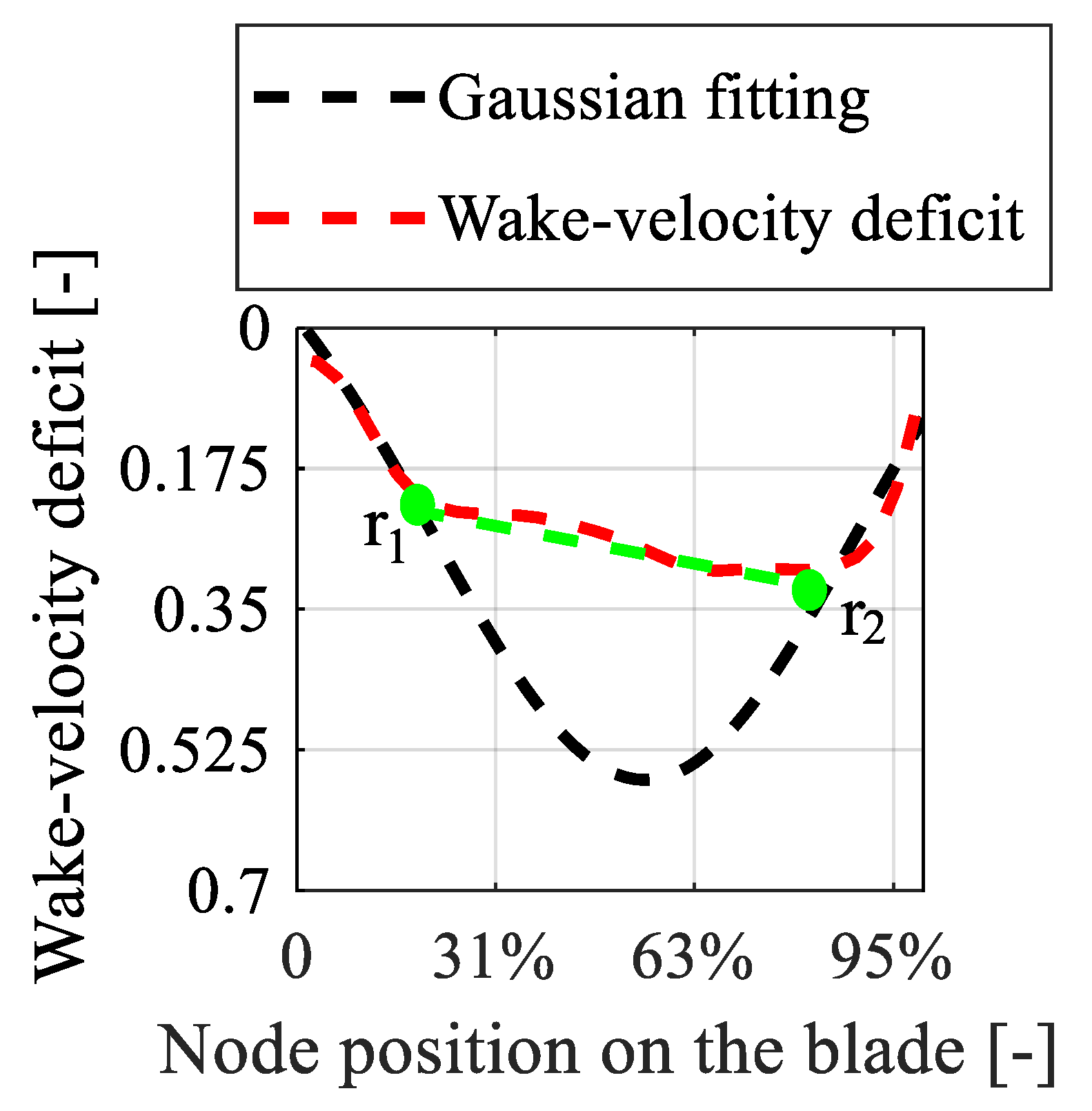
Establishment of a segmented functional initial wake profile behind the rotor: This study optimizes the profile contours near the extremum points in the near-wake region of the DG wake model. In this region, especially in areas close to the turbine, the wake profile contours are significantly influenced by the blades. Using the wake velocity distribution counter, the initial wake is approximated as a segmented function composed of Gaussian functions and straight lines, leading to a refined wake profile contour near the extremum points.

(2)

Correction of the wake spreading function: Considering the spatial transport of the wake as a flow duct, the study defines the flow duct exit position function and the expansion coefficient inside and outside the flow duct based on high-fidelity data identification. The wake spreading function is corrected according to the inside and outside of the flow duct. Combining the redefined near-wake region wake profile and the corrected wake spreading function, a three-dimensional Optimized-DG wake model is established. Validation using SOWFA and experimental data demonstrates the high accuracy of the Optimized-DG model.

(3)

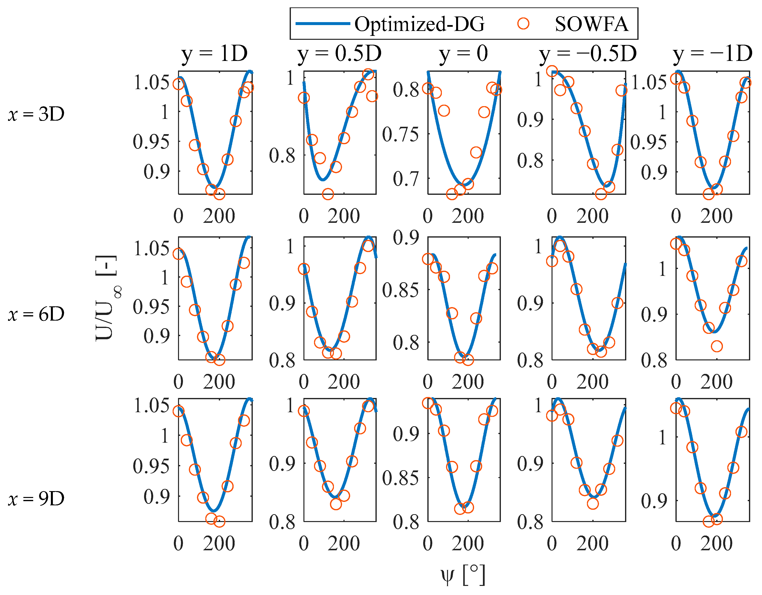
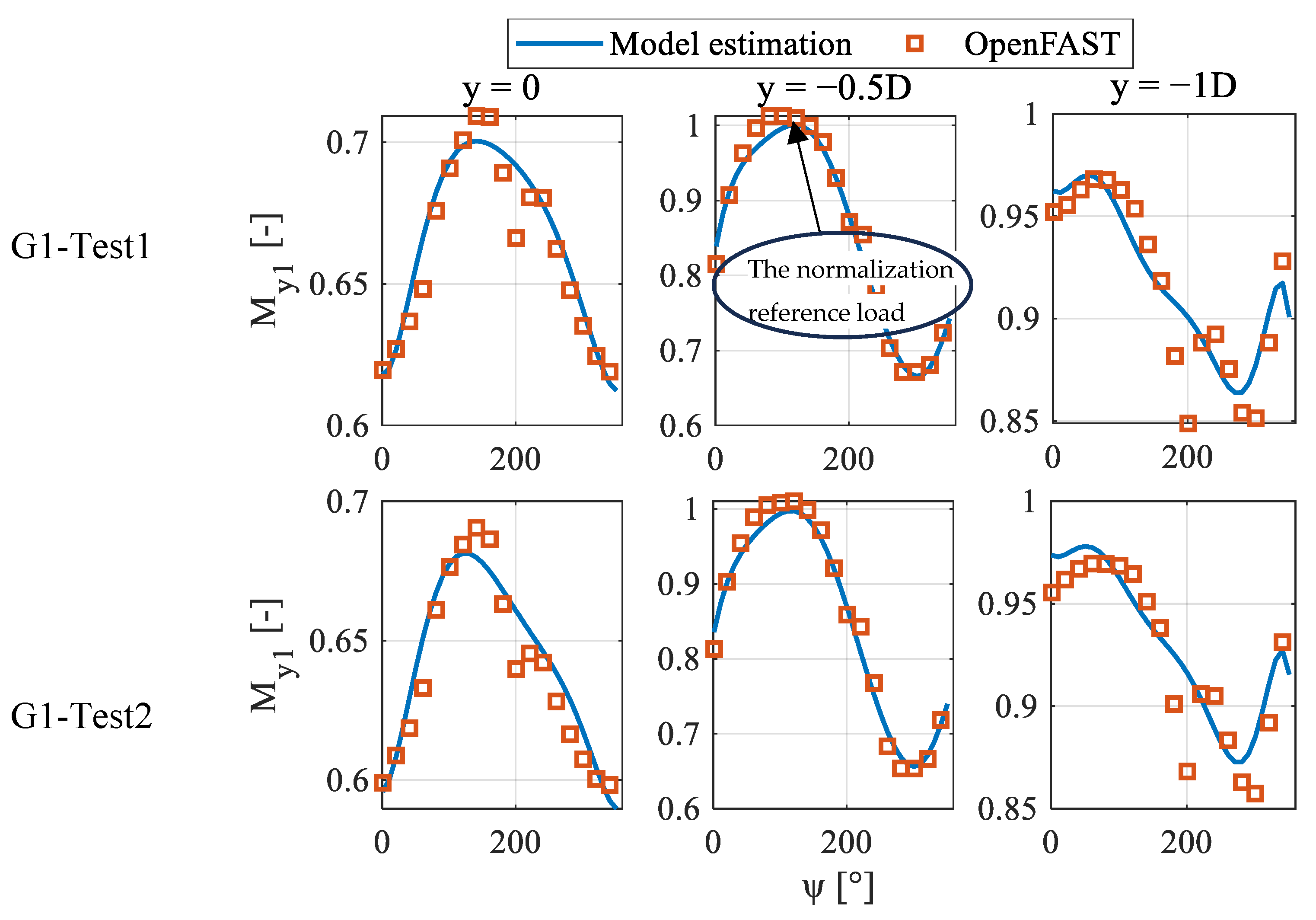
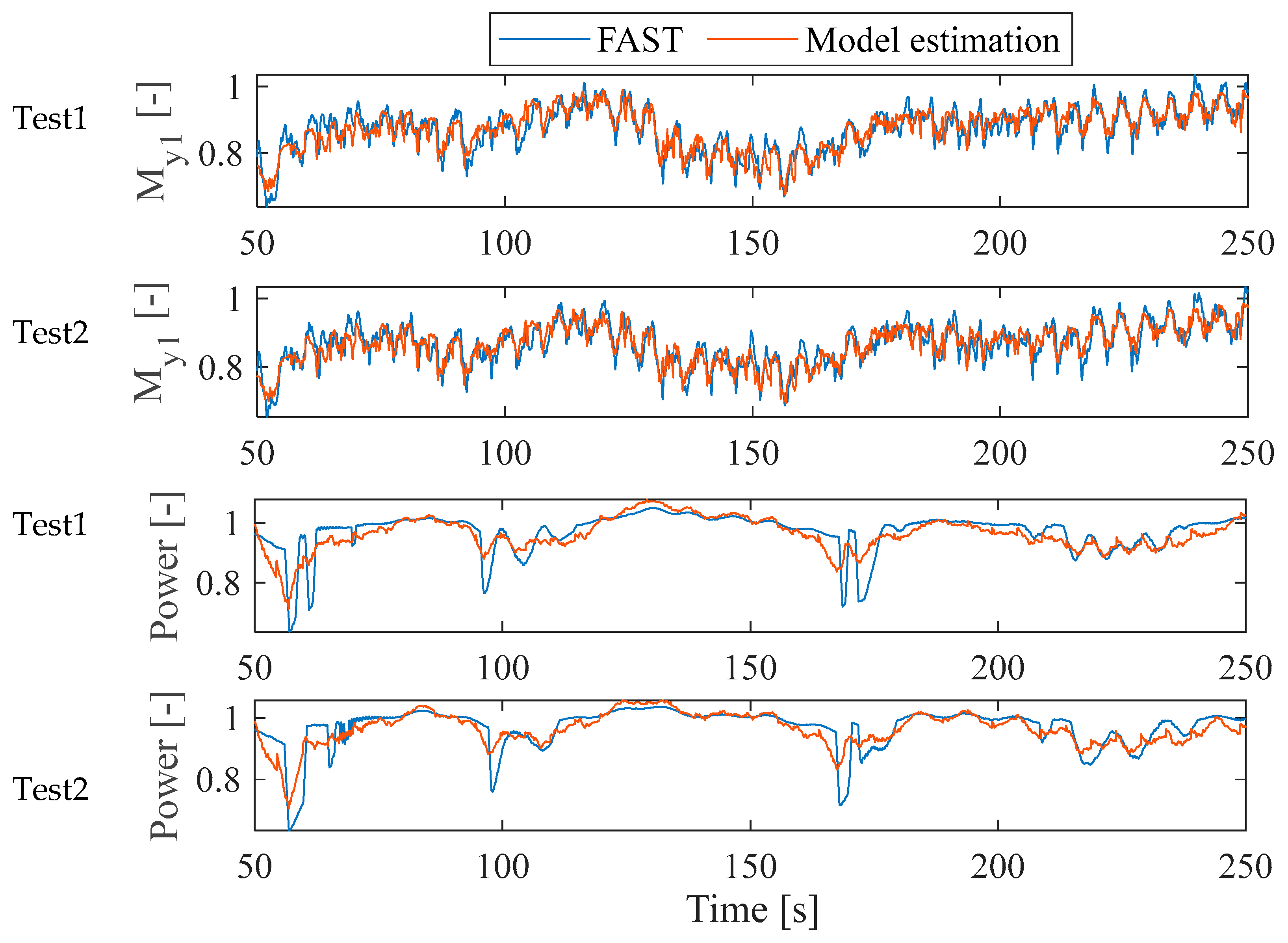
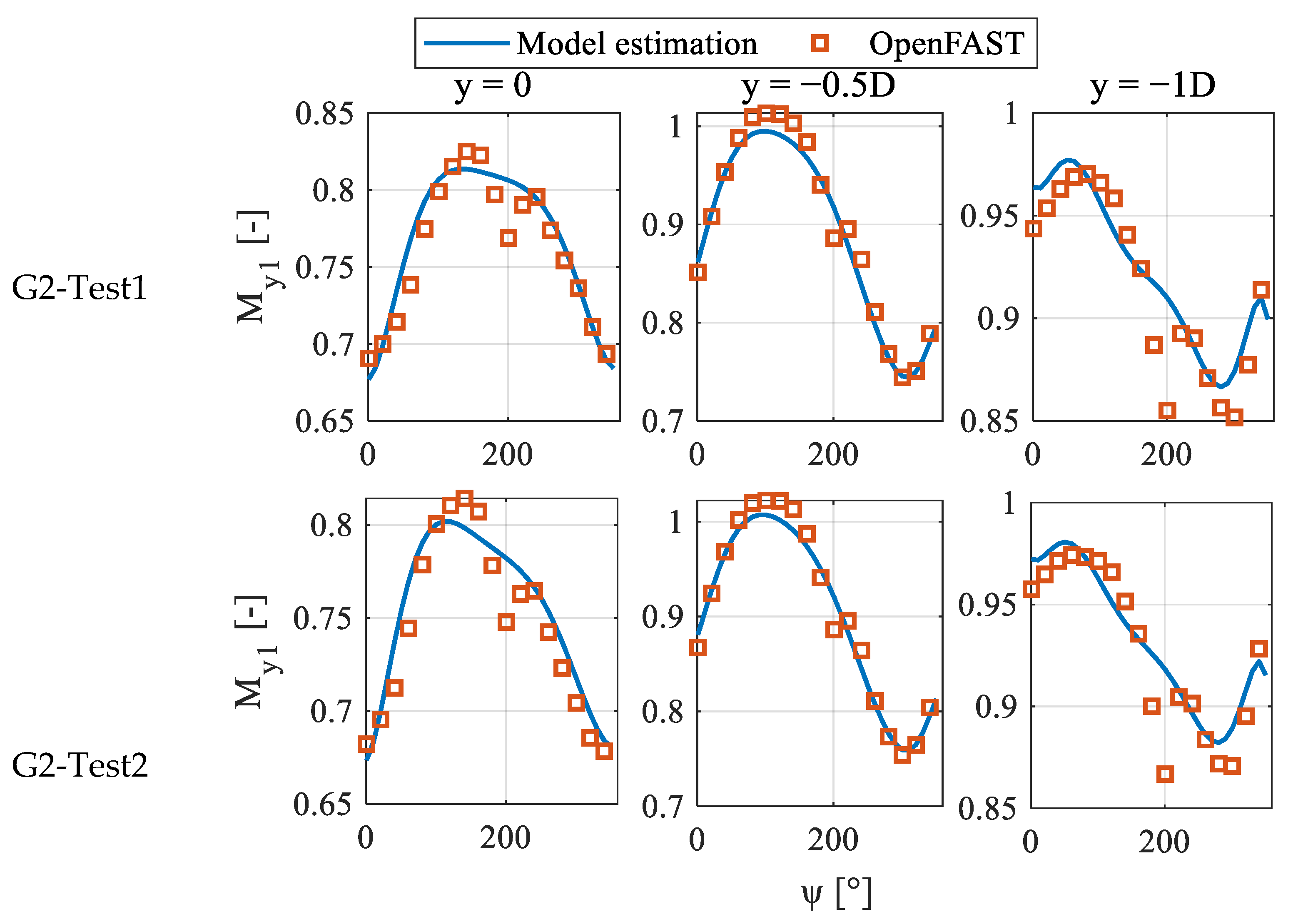
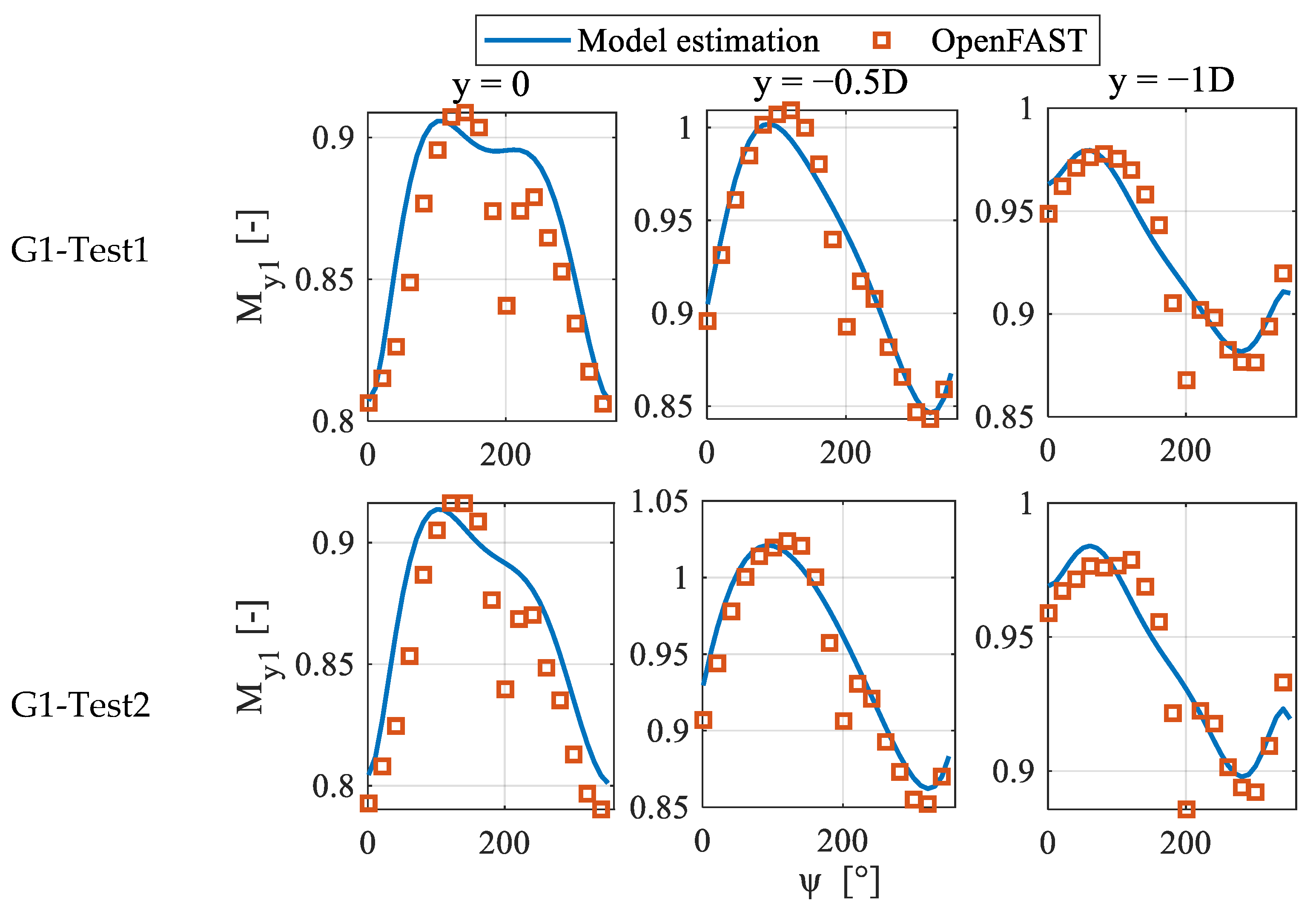
Introduction of a rapid calculation method for wind turbine fluctuating loads and power estimation under different wake interference: The fluctuations in wind turbine loads caused by wake interference exhibit periodicity, depending on wind turbine rotational speed, wind speed, pitch angle, blade azimuth angle, and wave height. Utilizing the Optimized-DG model for wake velocity prediction, the study provides a fast method to obtain the fluctuating loads varying with blade azimuth angle. Through OpenFAST validation, the proposed model estimation method achieves a maximum error of 10.02% and an average amplitude error of approximately 3.93% in predicting blade root flap-wise loads under wake interference. The maximum error in power estimation is 3%, with an average error of 1%.

Model limitations: All identified data in the simulation are obtained using the NREL 5 MW Base-Line simulation, so it is applicable to wind farms with turbine blades consistent with the NREL 5 MW Base-Line, so the model may not be applicable to others.

Outlook for Future Research: The rapid load calculation method for wind turbines based on the Optimized-DG model, proposed in this study, is suitable for quick load estimation in wake control scenarios. In future research, a wind farm wake control method will be developed that jointly considers wind turbine fluctuating loads and wind farm power.

References

1. Zhao, L.; Xue, L.; Li, Z.; Wang, J.; Yang, Z.; Xue, Y. Progress on Offshore Wind Farm Dynamic Wake Management for Energy. J. Mar. Sci. Eng. 2022, 10, 1395. [Google Scholar] [CrossRef]
2. Chanprasert, W.; Sharma, R.; Cater, J.; Norris, S. Large Eddy Simulation of wind turbine fatigue loading and yaw dynamics induced by wake turbulence. Renew. Energy 2022, 190, 208–222. [Google Scholar] [CrossRef]
3. Kim, S.-H.; Shin, H.-K.; Joo, Y.-C.; Kim, K.-H. A study of the wake effects on the wind characteristics and fatigue loads for the turbines in a wind farm. Renew. Energy 2015, 74, 536–543. [Google Scholar] [CrossRef]
4. Xue, L.; Wang, J.; Zhao, L.; Wei, Z.; Yu, M.; Xue, Y. Wake Interactions of Two Tandem Semisubmersible Floating Offshore Wind Turbines Based on FAST. Farm. J. Mar. Sci. Eng. 2022, 10, 1962. [Google Scholar] [CrossRef]
5. Zhao, L.; Gong, F.; Chen, S.; Wang, J.; Xue, L.; Xue, Y. Optimization study of control strategy for combined multi-wind turbines energy production and loads during wake effects. Energy Rep. 2022, 8, 1098–1107. [Google Scholar] [CrossRef]
6. Zhao, L.; Gong, Y.; Gong, F.; Zheng, B.; Wang, J.; Xue, L.; Xue, Y. Study on Mitigation of Wake Interference by Combined Control of Yaw Misalignment and Pitch. J. Mar. Sci. Eng. 2023, 11, 1288. [Google Scholar] [CrossRef]
7. Jonkman, J.M.; Shaler, K. Fast. Farm User’s Guide and Theory Manual; National Renewable Energy Laboratory: Golden, CO, USA, 2021. [Google Scholar]
8. Kretschmer, M.; Jonkman, J.; Pettas, V.; Cheng, P.W. FAST.Farm load validation for single wake situations at alpha ventus. Wind Energy Sci. Discuss. 2021, 6, 1–20. [Google Scholar]
9. Jensen, N.O. A Note on Wind Generator Interaction; Risø National Laboratory: Roskilde, Denmark, 1983. [Google Scholar]
10. Shakoor, R.; Hassan, M.Y.; Raheem, A.; Wu, Y.-K. Wake effect modeling: A review of wind farm layout optimization using Jensen׳s model. Renew. Sustain. Energy Rev. 2016, 58, 1048–1059. [Google Scholar] [CrossRef]
11. Archer, C.L.; Vasel-Be-Hagh, A.; Yan, C.; Wu, S.; Pan, Y.; Brodie, J.F.; Maguire, A.E. Review and evaluation of wake loss models for wind energy applications. Appl. Energy 2018, 226, 1187–1207. [Google Scholar] [CrossRef]
12. Bastankhah, M.; Porté-Agel, F. A new analytical model for wind-turbine wakes. Renew. Energy 2014, 70, 116–123. [Google Scholar] [CrossRef]
13. Li, L.; Huang, Z.; Ge, M.; Zhang, Q. A novel three-dimensional analytical model of the added streamwise turbulence intensity for wind-turbine wakes. Energy 2022, 238, 121806. [Google Scholar] [CrossRef]
14. Wang, T.; Cai, C.; Wang, X.; Wang, Z.; Chen, Y.; Song, J.; Xu, J.; Zhang, Y.; Li, Q. A new Gaussian analytical wake model validated by wind tunnel experiment and LiDAR field measurements under different turbulent flow. Energy 2023, 271, 127089. [Google Scholar] [CrossRef]
15. He, R.; Deng, X.; Li, Y.; Dong, Z.; Gao, X.; Lu, L.; Zhou, Y.; Wu, J.; Yang, H. Three-Dimensional Yaw Wake Model Development with Validations from Wind Tunnel Experiments. Energy 2023, 282, 128402. [Google Scholar] [CrossRef]
16. Gao, X.; Zhang, S.; Li, L.; Xu, S.; Chen, Y.; Zhu, X.; Sun, H.; Wang, Y.; Lu, H. Quantification of 3D spatiotemporal inhomogeneity for wake characteristics with validations from field measurement and wind tunnel test. Energy 2022, 254, 124277. [Google Scholar] [CrossRef]
17. Keane, A.; Aguirre, P.E.O.; Ferchland, H.; Clive, P.; Gallacher, D. An analytical model for a full wind turbine wake. Proc. J. Phys. Conf. Ser. 2016, 753, 032039. [Google Scholar] [CrossRef]
18. Keane, A. Advancement of an analytical double-Gaussian full wind turbine wake model. Renew. Energy 2021, 171, 687–708. [Google Scholar] [CrossRef]
19. Sadek, Z.; Scott, R.; Hamilton, N.; Cal, R.B. A three-dimensional, analytical wind turbine wake model: Flow acceleration, empirical correlations, and continuity. Renew. Energy 2023, 209, 298–309. [Google Scholar] [CrossRef]
20. Schreiber, J.; Balbaa, A.; Bottasso, C.L. Brief communication: A double-Gaussian wake model. Wind Energy Sci. 2020, 5, 237–244. [Google Scholar] [CrossRef]
21. Jonkman, J. The new modularization framework for the FAST wind turbine CAE tool. In Proceedings of the 51st AIAA Aerospace Sciences Meeting Including the New Horizons Forum and Aerospace Exposition, Grapevine, TX, USA, 7–10 January 2013; p. 202. [Google Scholar]
22. Churchfield, M.J.; Sang, L.; Moriarty, P.J. Adding Complex Terrain and Stable Atmospheric Condition Capability to the OpenFOAM-Based Flow Solver of the Simulator for on/offshore Wind Farm Applications (SOWFA); National Renewable Energy Laboratory (NREL): Golden, CO, USA, 2013. [Google Scholar]
23. Zhang, S.; Gao, X.; Lin, J.; Xu, S.; Zhu, X.; Sun, H.; Yang, H.; Wang, Y.; Lu, H. Discussion on the spatial-temporal inhomogeneity characteristic of horizontal-axis wind turbine’s wake and improvement of four typical wake models. J. Wind Eng. Ind. Aerodyn. 2023, 236, 105368. [Google Scholar] [CrossRef]
24. Sun, W.; Li, Y.; Shi, Q.; Ouyang, T.; Ma, L. Passive aeroelastic study of large and flexible wind turbine blades for load reduction. Structures 2023, 58, 105331. [Google Scholar] [CrossRef]
25. Jonkman, J.M.; Hayman, G.; Jonkman, B.; Damiani, R.; Murray, R. AeroDyn v15 User’s Guide and Theory Manual; NREL Draft Report; National Renewable Energy Laboratory: Golden, CO, USA, 2015. [Google Scholar]
26. Bottasso, C.; Cacciola, S.; Schreiber, J. Local wind speed estimation, with application to wake impingement detection. Renew. Energy 2018, 116, 155–168. [Google Scholar] [CrossRef]
27. Jonkman, J.; Butterfield, S.; Musial, W.; Scott, G. Definition of a 5-MW Reference Wind Turbine for Offshore System Development; National Renewable Energy Laboratory (NREL): Golden, CO, USA, 2009. [Google Scholar]
Figure 1. (a) Diagram of lift acquisition position and wake measurement position. (b) Three-dimensional wind speed measurement schematic.
Jmse 12 00647 g001aJmse 12 00647 g001b
Figure 2. Normalized data obtained from SOWFA; % represents the of node position on the blade span, the wake variation approximately follows a linear pattern (the green dashed line).
Jmse 12 00647 g002
Figure 3. The wake velocity distribution profiles at x = 1D to 3D.
Jmse 12 00647 g003
Figure 4. Comparison of normalized wind speeds on four horizontal profiles located at x     3 D .
Jmse 12 00647 g004
Figure 5. Comparison of normalized wind speeds on three horizontal profiles located at x > 3 D .
Jmse 12 00647 g005
Figure 6. Comparison of normalized wind speeds on six vertical profiles.
Jmse 12 00647 g006
Figure 7. RMSE comparison between wake models and CFD Data.
Jmse 12 00647 g007
Figure 8. BEM diagram.
Jmse 12 00647 g008
Figure 9. Time course diagram of wind (top) and wave (bottom).
Jmse 12 00647 g009
Figure 10. The time-history diagram of blade-root flap-wise load and power.
Jmse 12 00647 g010
Figure 11. Comparison of circumferential wind speeds of r = 2 3 R .
Jmse 12 00647 g011
Figure 12. Flowchart of rapid estimation process for blade-root flap-wise loads under wake disturbances.
Jmse 12 00647 g012
Figure 13. Load comparison between model estimates and OpenFAST results for the G1 simulation.
Jmse 12 00647 g013
Figure 14. Load comparison between model estimates and OpenFAST results for the G2 simulation.
Jmse 12 00647 g014
Figure 15. Load comparison between model estimates and OpenFAST results for the G3 simulation.
Jmse 12 00647 g015
Figure 16. Power comparison between model estimates and OpenFAST results for the G1–G3 simulation.
Jmse 12 00647 g016