Article

Enhancing Marina Sustainability: Water Quality and Flushing Efficiency in Marinas

by
Mohamad Alkhalidi
* and
Abdalrahman Alsulaili
Civil Engineering Department, Kuwait University, P.O. Box 5969, Kuwait City 13060, Kuwait
*
Author to whom correspondence should be addressed.
J. Mar. Sci. Eng. 2024, 12(4), 649; https://doi.org/10.3390/jmse12040649
Submission received: 14 March 2024 / Revised: 6 April 2024 / Accepted: 9 April 2024 / Published: 12 April 2024
(This article belongs to the Section Coastal Engineering)

Abstract

:
Coastal marinas are particularly susceptible to pollution due to their limited flushing capabilities and ineffective management practices. Therefore, it is necessary to implement measures that promote enhanced sustainability. This study aims to explore the intricate relationship between tidal flushing characteristics and water quality within marinas to foster sustainable development and management practices that mitigate environmental impacts. The research scrutinized seven marinas along the Kuwait coastline, each exhibiting unique hydrodynamic conditions and geometric configurations. Water quality indicators such as BOD, COD, DO, and SO42− were evaluated concerning each marina’s flushing efficiency through field assessments and hydrodynamic numerical modeling. An empirical formula was developed to predict and optimize flushing mechanisms, which provided critical insights into the design and management of marinas to enhance water quality. The study revealed significant disparities in water quality across the examined marinas as the hydrodynamic and geometric conditions differed. The empirical formula developed offers a novel approach to quantitatively assessing flushing efficiency, which is valuable for marina designers and managers, facilitating informed decisions, and promoting environmental sustainability. This study underscores the critical importance of integrating hydrodynamic and geometric considerations in the design and management of marinas to improve water quality and sustainability. It advocates for a multifaceted strategy that includes advanced design solutions, rigorous policy implementation, and active community engagement to safeguard coastal marine environments. The findings emphasize the need for comprehensive environmental management plans.

1. Introduction

The surge in coastal activities, particularly yacht and boat sailing, has seen exponential growth since the 19th century, reflecting a significant shift in economic and environmental dynamics [1]. With over 62% of major cities located along coastlines and more than half of the world’s population residing in coastal areas, the economic impact of these activities is profound [2,3]. In the United States, 11,500 marinas contribute $18 billion to the economy annually [4], and the maritime market in Kuwait shows robust growth, with boat and yacht sales increasing by 40% between 2012 and 2015.
This rapid growth mirrored global trends and underscored the urgent need to expand marinas to meet the increasing demand for berthing and maintenance services and bolster the tourism economy. However, such growth is not without its environmental consequences [5]. Although marinas, in general, pose a limited pollution threat to coastal environments [6,7,8], they are subjected to higher pollution levels than open seas when their natural flushing characteristics are inefficient. Pollutants in marinas include nutrients, pathogens, sediment runoff, and various wastes from boats, all of which can significantly impact marine ecosystems and water quality [8,9].
Research has shown that inadequate flushing and boating activities can trap pollutants and release substantial amounts of pollutants within marina basins, leading to concerning ecological effects such as plankton algal and red tide blooms [10]. Therefore, managing marinas is a challenge due to the sensitivity of coastal areas and the complexity of the marine environment. In response to growing public concern for coastal water quality and stricter legislative standards, there is an increasing emphasis on conducting environmental impact assessments and implementing improved management and design strategies for coastal systems [11,12,13,14]. These strategies, for example, must adapt state-of-the-art design solutions to protect coastal systems and improve water circulation, such as engineering-with-nature systems that fulfill the requirements of high levels of protection, sustainability, and pleasing natural aesthetics [15] or slotted vertical and sloped structures [16,17] that provide protection and increase the water exchange between ambient and marina water.
The central objective of this study is to explore the relationship between tidal hydrodynamics in marinas and the consequent water quality. The study aims to bridge the knowledge gap regarding this interplay by examining the factors influencing the flushing capabilities of marinas. Also, the study proposes sustainable pollution control measures informed by these findings, providing a foundation for environmental management and policy development decision-making. The research employs an approach that includes field assessments, numerical modeling, and the development of sustainable measures. Hence, seven marinas along the Kuwait coastline have been chosen for this study, representing a variety of hydrodynamic conditions and geometric configurations.
The manuscript is divided into five sections. Section 2 is a literature review of marine and marina pollution and flushing characteristics; Section 3 elaborates on the methodology used, including details of the field campaign and the hydrodynamic and transport numerical models; Section 4 discusses the results; and Section 5 concludes the study.

2. Literature Review

Effective water exchange between the marina and its surrounding environment is crucial for enhancing the marina basin’s water quality and protecting boats and yachts from damage, as the water quality within marinas is closely linked to the extent of tidal exchange [18,19]. However, complex layouts and entrance configurations in marinas often hinder the interchange and mixing of ambient water, leading to increased pollutant concentrations and water quality degradation [20]. This understanding has led researchers and designers to recommend smoother and less irregular marina designs, as sharp corners and irregularities create stagnation points that impede water mixing and flushing [20].
The leading water quality indicators to assess the water quality inside marinas are the biological oxygen demand (BOD), chemical oxygen demand (COD), metals, and hydrocarbons, along with total dissolved solids (TDSs), water temperature (Tw), salinity (Sw), pH, and sulfate (SO42−) [8,21]. Low DO levels, accompanied by high BOD and COD, typically signify increased organic matter and potential pollution as they reflect higher oxygen consumption by microorganisms and the oxygen needed to oxidize organic matter in water. A low BOD/COD ratio indicates harm to the marine environment and ecosystem due to organic substances becoming unsuitable for biological treatment, with ratios above 0.4 or 0.5 indicating high biodegradability, 0.2–0.4 suggesting low biodegradability, and below 0.1 pointing to the presence of organics unsuitable for biological treatment [22,23,24]. Non-biodegradables, such as fats, oils, and greases [25], possibly discharged from boats, lower the BOD/COD ratio. They create a barrier, blocking microbial access to biodegradable material, and are resistant to biological degradation.
The water quality of marine systems can also become damaged due to the increased TDS, as it limits their ability to support biodiversity and the ecosystem and reduces the environmental security of recreational activities [26]. Climate change and increased urban development have been associated with rapid increases in TDS and significant environmental changes in the marine environment. These alterations can contribute to the proliferation of harmful algae and extreme turbidity, potentially leading to substantial economic losses and adverse health outcomes, as documented in several studies [26].
Finally, SO42− contamination in water environments has become increasingly prominent due to industrialization and urbanization, receiving more attention from researchers and managers [27,28]. The rising concentration of SO42− in water threatens human health and ecological balance, can be corrosive to materials, and indicates seawater and soil pollution [29,30,31]. In addition, algae and bacteria can overgrow with high SO42− levels, deteriorating boat hulls and metal fittings.
Therefore, improving water quality in marina basins requires identifying and mitigating pollution types and sources and enhancing flushing capabilities [32,33,34,35]. Optimal marina designs facilitate efficient flushing, typically achieved within two to four days in well-designed marinas, according to [36,37] and up to seven days, according to [38]. In literature, entrance width plays a critical role in this process, with wider entrances promoting shorter flushing times [20,39]. Additional factors impacting flushing efficiency include marina layout, depth, tidal range and currents, wind and wave climate, and geographical location [32,40].
Efficient flushing time, tf, is the time required for pollutant concentrations to drop to about 37% of their original levels [18], and it can be calculated using several models and equations, each based on different assumptions and parameters. In scenarios where freshwater discharge is negligible, tidal action becomes the primary driving force for marina water flow and flushing efficiency [41,42,43,44]. Ref. [45] provided a formula to estimate tf for a tidal embayment as follows:
t f = 1.5 l w A h w + A l w R t
where ∀lw is the basin volume during low tide, Alw and Ahw are the basin surface areas at low and high tide, respectively, and Rt is the tidal range during spring tide. Equation (1) assumes that tf is when 60% of the original water is replaced with new water and that the mean tidal range over the year is approximately 70% of the spring tidal range [46]. Ref. [47] introduced another method for calculating tf, focusing on the mass of a scalar object and its mass flux as follows:
t f = M M ˙
where M is the mass of a scalar object and M s ˙ is the mass flux of a pollutant inside the basin. Refs. [48,49] recommend an alternative approach, especially when only the tidal prism and range are available. This approach involves the tidal prism P, mean basin volume ∀, a modification factor k, and the tidal period T, as follows:
t f = T 1 k P
The modification factor accounts for the proportion of water returning to the marina basin during flood tide and ranges between 0 and 1.
For the concentration of substances inside marinas [44], proposed empirical equations based on the tidal prism theory for different scenarios to calculate the substance rate of change of concentration d c d t and concentration c, inside a small water basin as follows:
d c d t = M s ˙ k ~ c 1 t f c c a m b I c c I
d c d t = c k ~ + 1 t f + I
d c d t = c 1 t f I = c 1 k P T I
c = c o e x p k ~ + 1 t f + I t
c = c o e x p 1 k P T I t
c = c o e x p k ~ + 1 t f t
c = c o e x p 1 k P T t = c o e x p t t f
where t is time, k ~ is the decay rate of the pollutant in 1/time, c a m b is the pollutant concentration in the ambient water outside the basin, I is the inflow rate in the case of the existence of a source point, and c I is the pollutant concentration in the inflow. Equations (5)–(10) are based on Equation (4). Equation (5) is for the case when c a m b = 0 ,   c I = 0 ,   a n d   M s ˙ = 0 , and when the polltant is a conservative pollutant, k ~ = 0 , Equation (5) becomes Equation (6). Equations (7)–(10) are the integration of Equations (5) and (6), assuming that the initial concentration inside the marina is c o at t = 0 , where Equations (9) and (10) represent the case of only tidal flow, i.e., I = 0 . Ref. [50] generalized these concepts in Equation (11).
c = c o e x p Q t
Equations (4)–(11) assume a well-mixed basin with no return of pollutants during flood tide. Equations (7)–(11) are exponential, indicating that any initiated pollution will never completely leave the basin. Researchers propose other empirical equations based on the specific conditions and assumptions listed in [18].
While empirical equations are helpful for small basins, they may yield significant errors in larger water bodies like bays [46]. They provide initial estimates of flushing behavior but are often complemented by sophisticated numerical models for more accurate results [51,52]. Though less common due to cost and facility requirements, physical models are valuable for complex flow patterns.
This research employs the use of MIKE 3 version 2023, a comprehensive hydrodynamic and transport simulation software developed by the Danish Hydraulic Institute (DHI), to analyze the hydrodynamic and flushing characteristics of marinas. The numerical modeling is supplemented with the field campaign results to assess the spatial and temporal variations of key water quality parameters, offering insights into the environmental health of the marinas and relating it to the flushing efficiency.

3. Methodology

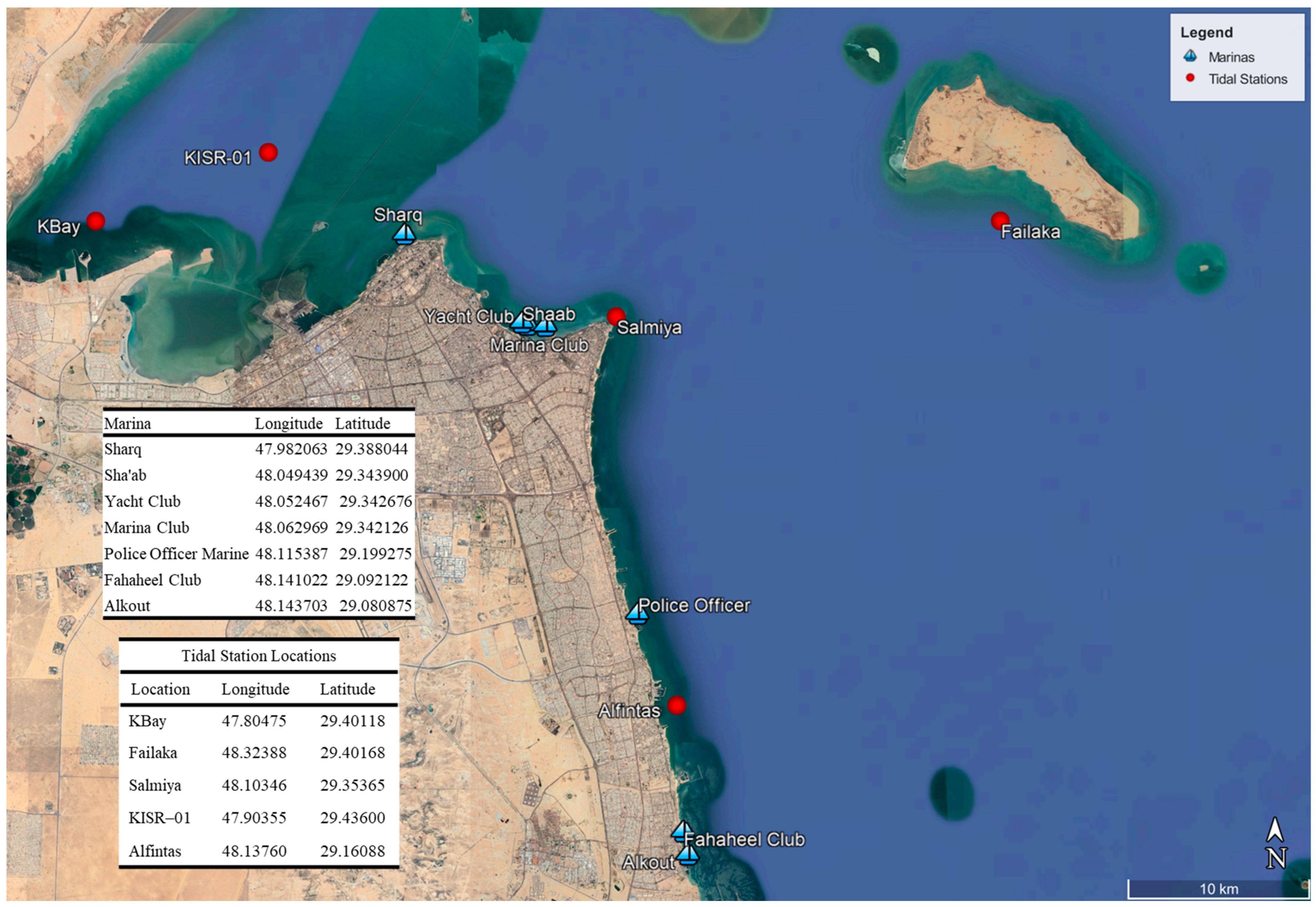
3.1. Field Data Sampling and Measurements

The field campaign monitored water quality indicators, including DO, BOD, COD, TDS, Tw, Sw, pH, and SO42−. The YSI Professional Plus handheld meter and the Castaway-CTD were utilized to measure the DO, Tw, Sw, and pH. The monitoring and sampling activities were carried out within all marinas, excluding the Police Officer Marina location due to construction activities, from May to October 2020. The sampling locations are depicted in Figure 1.
The TDS was measured using the USEPA 160.1 method [53], while the. BOD, COD, and SO42− concentrations were determined using the 5210B, 5220D, and 4500-SO42− methods, respectively [54]. These methods encompass the sampling and analytical procedures required to determine these parameters accurately under specified conditions.
One hundred fifty-six samples were collected from various marinas, with each marina visited 3 to 4 times to ensure comprehensive spatial coverage. Within each marina basin, 6 to 8 sampling locations were chosen (detailed data are provided in Appendix A). The samples were analyzed at Kuwait University’s Department of Civil Engineering Environmental Laboratory and the National Unit of Environmental Research and Services (NURES). Figure 2 presents the maximum, minimum, and average values of TDS, BOD, COD, and SO42− for all marinas, while Figure 3 illustrates the calculated maximum, minimum, and average BOD/COD ratios.

3.2. Numerical Models

3.2.1. Model Description

The MIKE 3 Flexible Mesh Hydrodynamic (M3 FMHD) model was utilized to investigate the hydrodynamic characteristics of Kuwait’s territorial waters and marinas, focusing on tidal currents and surface elevation. This model employs the three-dimensional incompressible Reynolds averaged Navier–Stokes equations, integrating the Boussinesq and hydrostatic pressure approximations for modeling buoyancy-driven flows [55]. The model includes conservation equations for mass, momentum, temperature, and salinity, complemented by a turbulent closure scheme, and uses the Smagorinsky formulation for horizontal eddy viscosity and the log law or k-ϵ formulation for vertical eddy viscosity [55]. The governing equations of the M3 FMHD are [55] as follows:
The local continuity equation is as follows:
u x + v y + w z = S
The horizontal x and y components of the momentum equation are as follows:
u t + u 2 x + v u y + w u z = f v g η x 1 ρ P a x g ρ z η ρ x d z 1 ρ h s x x x + s x y y + F u + z V t u z + u s S
v t + v 2 x + v u y + w v z = f u g η y 1 ρ P a y g ρ z η ρ y d z 1 ρ h s y x x + s y y y + F v + z V t v z + v s S
The horizontal stress terms F u and F v are described by gradient–stress relations as follows:
F u = x 2 A u x + y A u y + v x
F v = y 2 A v y + x A u y + v x
In the hydrodynamic module, calculations of the transports of temperature T and salinity s follow the general transport–diffusion equations as follows:
T t + u T x + v T y + w T z = F T + z D v T z + H ^ + T s S
s t + u s x + v s y + w s z = F s + z D v s z + s s S
The terms in Equations (12)–(18) are listed in Table 1.

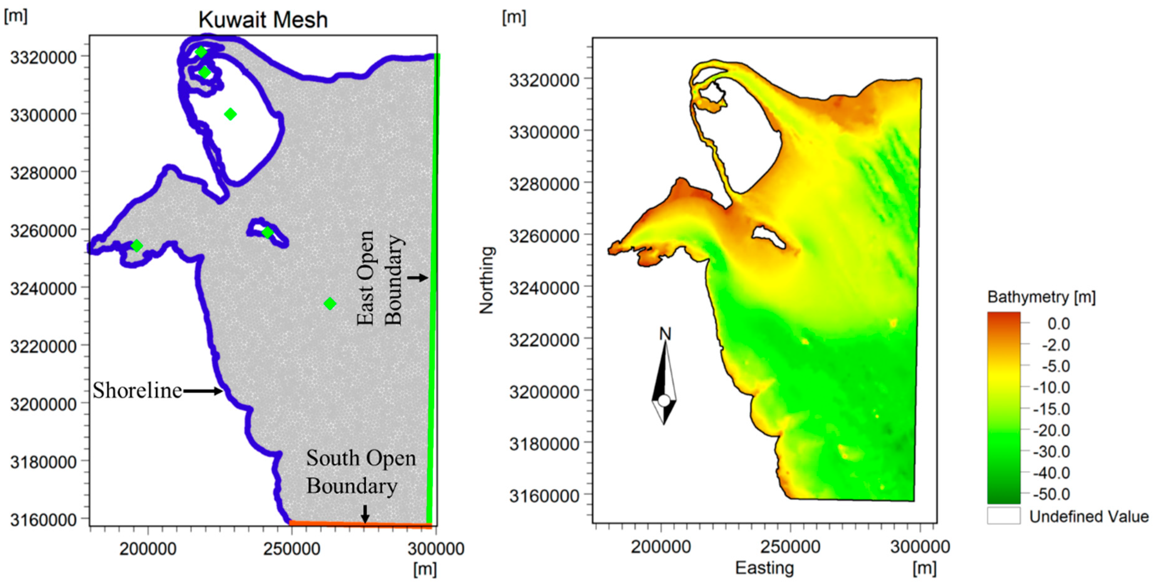
3.2.2. Kuwait’s Hydrodynamic Model (KHDM) Setup

The KHDM features a flexible mesh that accurately depicts coastal regions with horizontal, unstructured, and vertically structured elements. This configuration facilitates refined meshing near complex land boundaries, enables precise resolution, and increases accuracy [56]. The model’s reliability depends on the mesh quality and boundary conditions, as coarse meshes and inaccurate boundary conditions can increase numerical errors [56].
The mesh setup, depicted in Figure 4, consists of ten layers of Sigma coordinates, comprises 31,296 nodes and 60,945 elements horizontally, and layer thickness varies from 5% near the surface to 20% at intermediate layers, as recommended by [57]. The maximum element area was 1.409 × 10⁶ m2, the minimum was 9487 m2, and the smallest allowable angle was 26 degrees. Bathymetric data were sourced from Admiralty Charts and MIKE CMAP and adjusted to MSL [58], and the mesh is projected onto the Universal Transverse Mercator 39 (UTM-39) coordinate system. Boundary and initial conditions were derived from the Boundary Conditions Generator for MIKE 3 [59]. Table 2 summarizes water level characteristics at each boundary and Figure 5 shows water level and salinity boundary conditions at the centers of the south and east boundaries.
The KHDM model’s basic input parameters from the previous study [57] and calibration processes are listed in Table 3. The model also incorporates heat exchange parameters for meteorological conditions. For the latent heat, the default values of constant in Dalton’s law, wind coefficient in Dalton’s law, and critical wind speed of 0.5, 0.9, and 2 m/s, respectively, were used. The default values of heating and cooling transfer coefficients of 0.0011 were used for sensible heat. The light extinction parameter was set to 1.4 for the short-wave radiation, and the Beta in Beer’s Law was kept at the default value of 0.3. For long-wave radiation, the calculations of the long-wave radiation were set as “empirical” in the model. The air temperature, relative humidity, and the 10 m u- v-components wind data were obtained from the European Centre for Medium-Range Weather Forecasts (ECMWF)—ERA5 hourly data on single levels [60]. Figure 5 shows samples of the relative humidity (e) and air temperature (f) at the center of the Kuwait Bay entrance during November 2017. The wind’s direction is mainly from the northwest, north, and northeast directions (Shamal wind), as indicated in the wind rose plot shown in Figure 5g. The model’s wind friction was set to vary linearly with the wind speed, and the friction was set to be 0.0006 at a wind speed of 0 and 0.0027 at 25 m/s [57].
The discharge from the desalination plants was also included in the model as source points: volume discharge, salinity, and temperature. The stations included Doha East, Doha West, Shuwaikh, AlSubiya, AlShuaiba, and Alzour power and desalination plants. The specifications of the source points listed in Table 4 are based on [57] and personal communications with the Ministry of Electricity and Water, Kuwait. All points were forced onto the surface layer of the model.

3.2.3. Calibration and Validation Process

The KHDM was simulated for calibration and validation over various periods. The details of the simulations, including measurement locations, simulation and data measurement periods, and types of data measured, are outlined in Table 5. Figure 1 illustrates the geographical distribution of tidal measurement locations. Each simulation began with a 30-day ‘cold start’ phase, allowing the model to establish real-time initial conditions and reach statistical equilibrium. During this phase, the models started with zero surface elevation and tidal currents, while water temperature and salinity were set according to the start time of each simulation.
The model’s adaptive time step was set between a minimum of 0.01 s and a maximum of 30 s. Adjustments to the time step during the simulation were made to comply with the Courant–Friedrichs–Lewy (CFL) criterion, which limits the wave’s movement across a cell boundary within a single time step, thereby ensuring simulation stability [61]. In this study, the CFL number was maintained below 1, specifically at 0.8, to guarantee the simulation’s reliability.
A semi-implicit approach was used for time integration in the shallow water and transport (advection-dispersion) equations. This method explicitly treats horizontal terms, while vertical terms are handled implicitly [55]. Such an approach is designed to manage the complex dynamics within the model’s environment efficiently.

3.2.4. Hydrodynamic and Transport Numerical Modeling Setup for Marinas

Marinas were modeled using fine meshes, where element sizes were explicitly tailored, ranging from 5 m within to 300 m outside the marinas. The boundary conditions for these meshes were derived from the validated KHDM model. The interior of the marina basins features a maximum element area of 10 m2, while the area outside the marinas is set at a maximum of 4800 m2. A single refined flexible mesh was created for the closely situated Shaab, Yacht, and Marina Club Marinas. Similarly, a fine mesh was developed for the adjacent Police Officer, Fahaheel Club, and Alkout Marinas. All meshes include three open boundaries. Unique to Sharq Marina, there is a navigation channel that is 3 m deep and extends 1600 m northwest from its entrance. The specific characteristics of each marina are detailed in Table 6.
The transport module simulated the concentration of a tracer within the marinas, assuming an initial concentration of 100% inside the marinas and 0% outside (Figure 6). The model ran for 16 days to encompass complete tidal cycles, focusing on outputs like surface elevations, tidal currents, and tracer concentration.
For the transport model, the conservation equation for a scalar quantity is given by the following equation [55]:
C t + u C x + v C y + w C z = F C + z D C ν C z κ p C
where C is the concentration of the scalar quantity, kp is the linear decay rate of the scalar quantity, D C ν is the vertical turbulent (eddy) diffusion coefficient, and FC is the horizontal diffusion term. FC is given by the following equation:
F C = x D C h C x + y D C h C y
where D C h is the horizontal turbulent (eddy) diffusion coefficient. D C ν and D C h can be scaled by eddy viscosity or a constant.

4. Results and Discussion

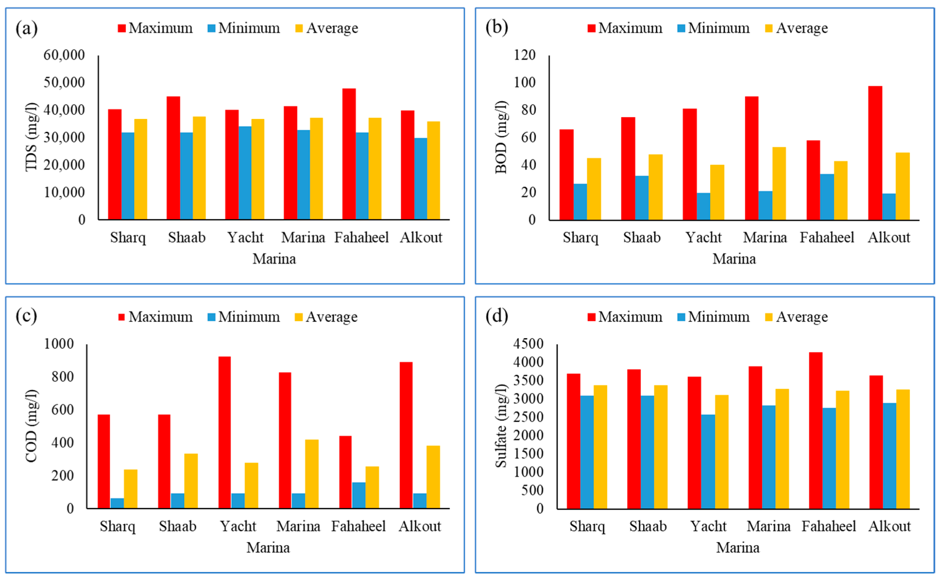
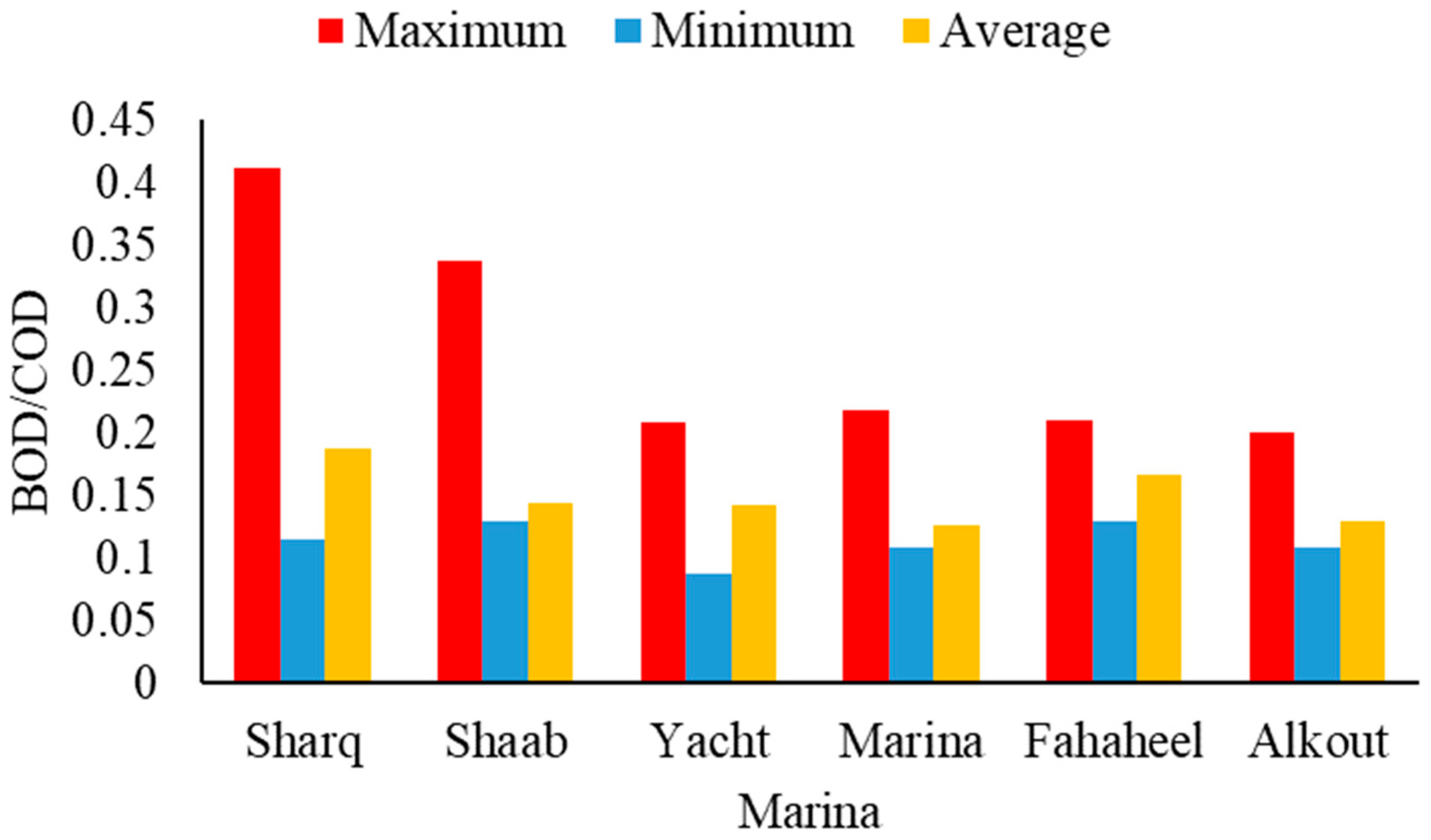
4.1. Water Quality Inside the Marinas

The field campaign uncovered significant insights into the water quality of tidal marinas, revealing deviations from established standards and fluctuations across various parameters. Generally, the water quality in the marinas fell short of the seawater quality standards outlined in local and international regulations [13,21,62]. While TDS levels mostly adhered to standard limits [63], exceptions were noted in Shaab and Fahaheel Marinas (Figure 2a). The pH levels remained within KEPA guidelines, ranging from 8.16 to 8.55 (Table A2). However, BOD and COD levels generally exceeded KEPA’s maximum limits for pollutants in wastewater discharged into the sea, set at 30 mg/L and 200 mg/L, respectively [13,21,24], with significant variations observed among marinas (Figure 2b,c).
Additionally, DO levels showed low and varied readings across the marinas, with most averaging below KEPA’s threshold of 4 mg/L, particularly notable during the summer (Table A1). Temperature readings, Table A2, ranged from 19.8 °C in Sharq Marina (October) to 39.2 °C in Alkout Marina (September), while salinity levels, Table A1, ranged between 39.29 PSU and 43.8 PSU. These temperature and salinity variations are consistent with Kuwait’s extreme climate, characterized by air temperatures fluctuating from near zero in January to over 50 °C from late June onwards [64] and high salinity levels attributed to factors such as intense evaporation rates during summer, sluggish water circulation during tidal periods, and brine water discharge from power and desalination plants.
At Alkout Marina, BOD levels exhibited significant variation, ranging from the lowest recorded value of 19.20 mg/L to the highest of 97.50 mg/L, with an average of 49.34 mg/L, the second-highest among all marinas sampled. Conversely, the Yacht Club Marina showcased the lowest average BOD of 40.1 mg/L, while the Marina Club Marina exhibited the highest average of 53.06 mg/L. Notably, extreme levels of BOD were observed within Alkout Marina, indicating potential areas of concern for organic pollution. Similarly, COD levels peaked at the Yacht Club, Marina Club, and Alkout Marinas, surpassing those of other sampled locations. On average, COD concentrations ranged from 239.67 mg/L at Sharq Marina to 421.13 mg/L at Marina Club Marina.
The elevated levels of BOD and COD observed in the marinas raise significant environmental concerns, primarily indicating the presence of organic pollutants. These pollutants can profoundly affect water quality by depleting DO, potentially leading to hypoxic or anoxic conditions detrimental to aquatic life [65,66]. Notably, Alkout Marina has been identified as experiencing chronic hypoxia, posing a substantial risk to aquatic ecosystems, as corroborated by a recent study [14].
Moreover, high COD levels often signify an abundance of nutrients, such as nitrates and phosphates, which can contribute to eutrophication. This excess nutrient input stimulates the overgrowth of algae and phytoplankton, leading to algal blooms that disrupt the balance of the ecosystem and impede the growth of aquatic plants [67]. Such disturbances can have far-reaching consequences for aquatic biodiversity and ecosystem functioning.
The average DO levels ranged from 1.74 mg/L (Sharq Marina) in May to a maximum of 5.55 mg/L (Yacht Club Marina) in October, showing seasonal variation accompanied by high levels of BOD and COD. Alkout Marina had consistently low DO levels, below 3 mg/L, throughout all measurements. There have been only a few instances where high maximum DO levels have been measured, and the cause remains unknown (Table A1).
The DO, BOD, and COD levels observed across all marinas consistently surpass local and global standards, indicating persistent pollution issues [8,21,68]. With the absence of identified wastewater sources, contamination likely arises from tidal water influx and improper waste disposal from boats, accompanied by inadequate natural flushing and exacerbated by elevated temperature and salinity levels that further deplete DO levels, particularly during the peak sailing season in summer [36,68].
Disposing of human fecal waste from boats significantly contributes to this issue, especially in marinas with poor flushing. The impact is substantial, with a single sewage discharge from a boat equivalent to approximately 10,000 household flushes [69]. Moreover, it has been estimated that a typical boat releases 130 million coliform bacteria and 5 g of oxygen-demanding material per operational hour [20].
Extreme cases observed in poorly flushing marinas have reported chlorophyll-a levels exceeding 25 mg/L and a drop in DO levels to 2 mg/L, leading to plankton algal and red tide blooms [10]. Such low DO levels can induce lethal and sublethal toxicity in the water column [68], promote the accumulation of organic materials in bed sediments, and elevate sediment oxygen demand, further exacerbating DO depletion [68,70,71].
Additionally, the observed BOD/COD ratios in the marinas are concerning, with maximum average ratios reaching 0.4185 and minimum ratios at 0.0873, with an overall average of 0.15, indicating resistance to conventional biological treatment methods [72]. These high ratios often signify the presence of non-biodegradable pollutants, including fats, oils, and greases, potentially originating from boats and yachts, posing significant risks to marine ecosystems [22,23,24]. Moreover, the observed BOD/COD ratios may indicate the presence of toxic pollutants within the marinas.
Figure 2d illustrates the variability in SO42− concentrations among different marinas, with levels ranging from 4279 mg/L at Fahaheel Marina to 2582 mg/L at Yacht Club Marina. The data reveals relatively consistent SO42− levels across marinas, with Yacht Club Marina recording the lowest average concentration (3110 mg/L) and Shaab Marina the highest (3379 mg/L). Notably, significant rusting observed on boat and yacht hulls during field observations at Fahaheel Marina aligns with studies associating high SO42− concentrations with accelerated algae and bacteria growth, leading to degradation of marine infrastructure [27,28,29,30] and indicating seawater and soil pollution [31].
In conclusion, this field study emphasizes the intricate relationship among various water quality parameters in marinas and underscores the urgent need for effective waste management practices. Implementing efficient waste flushing and disposal measures is crucial for protecting marine ecosystems and preventing damage to boats and yachts. Comprehensive environmental management strategies are essential to ensuring the sustainability and health of these vital marine environments.

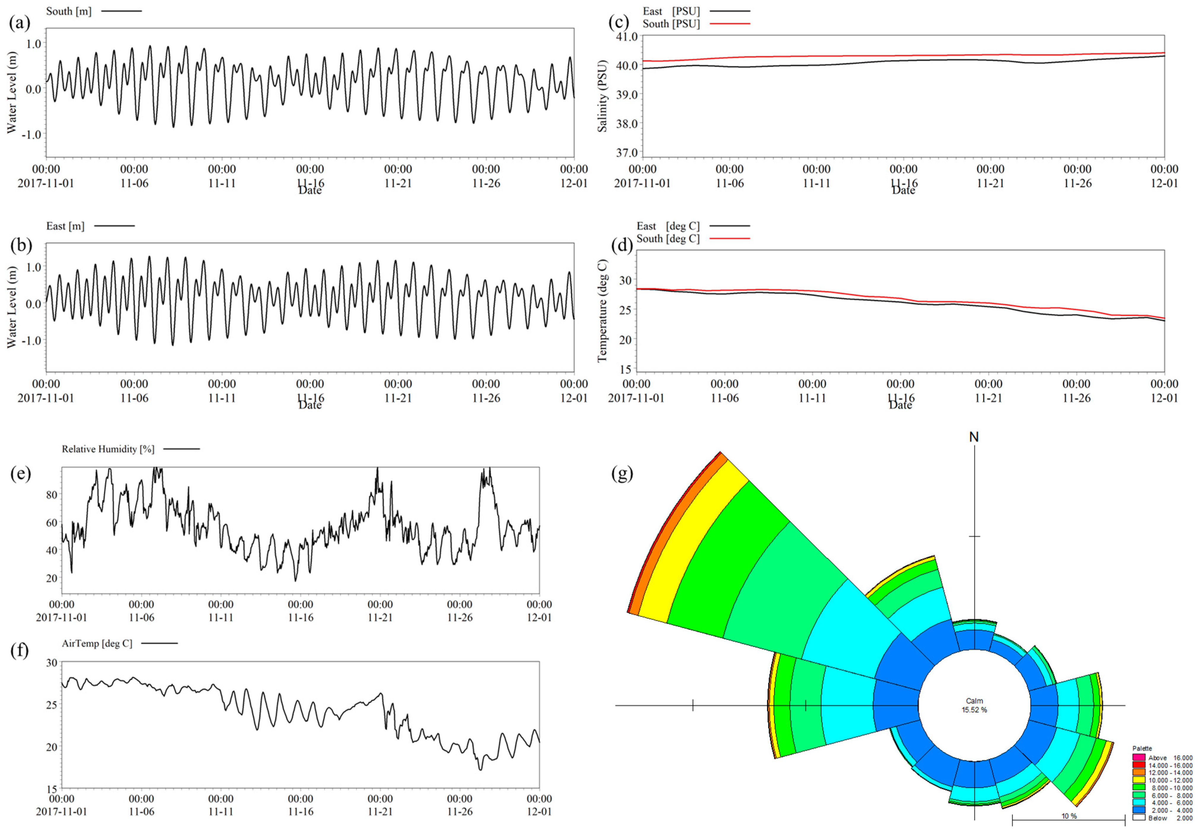
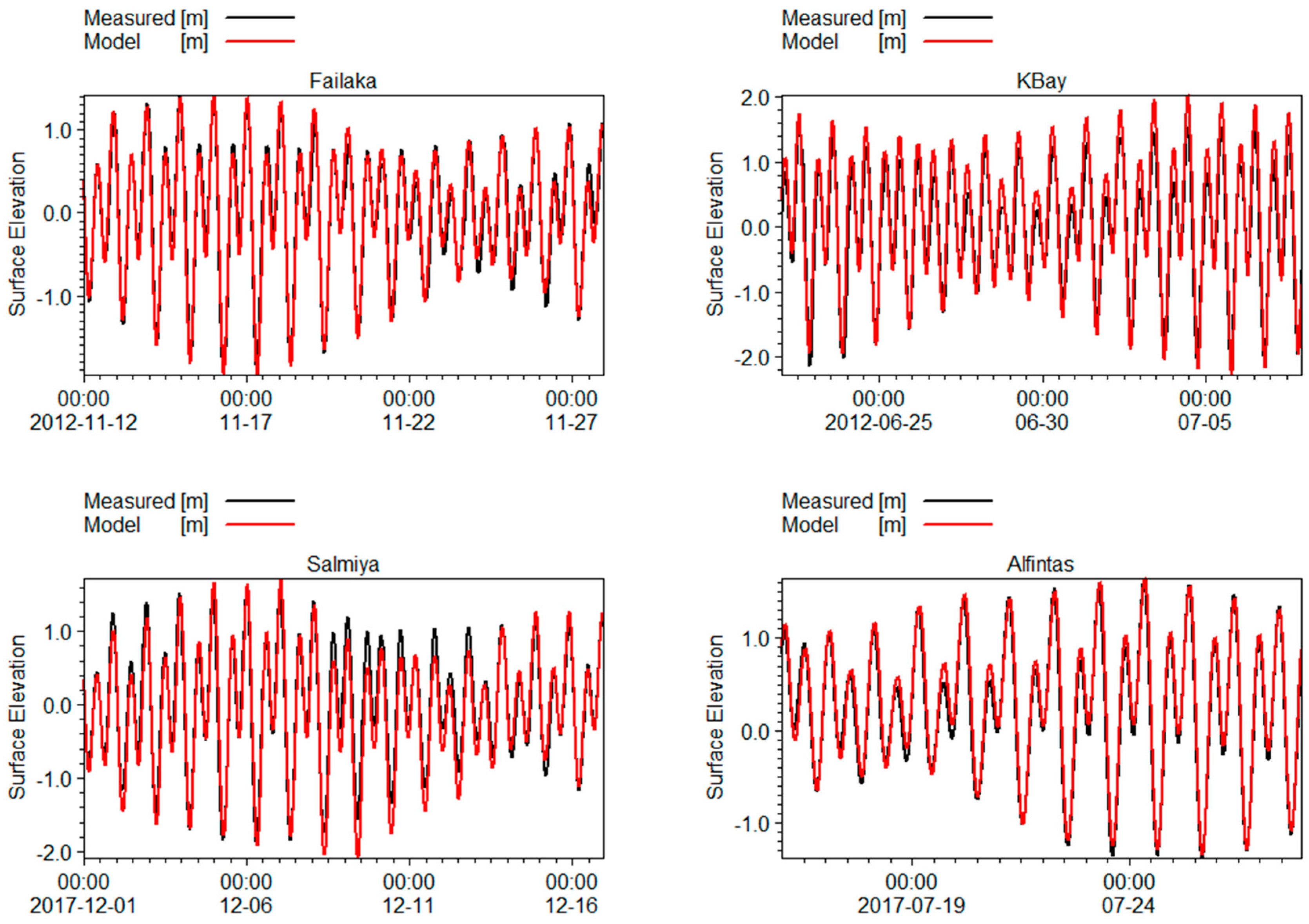
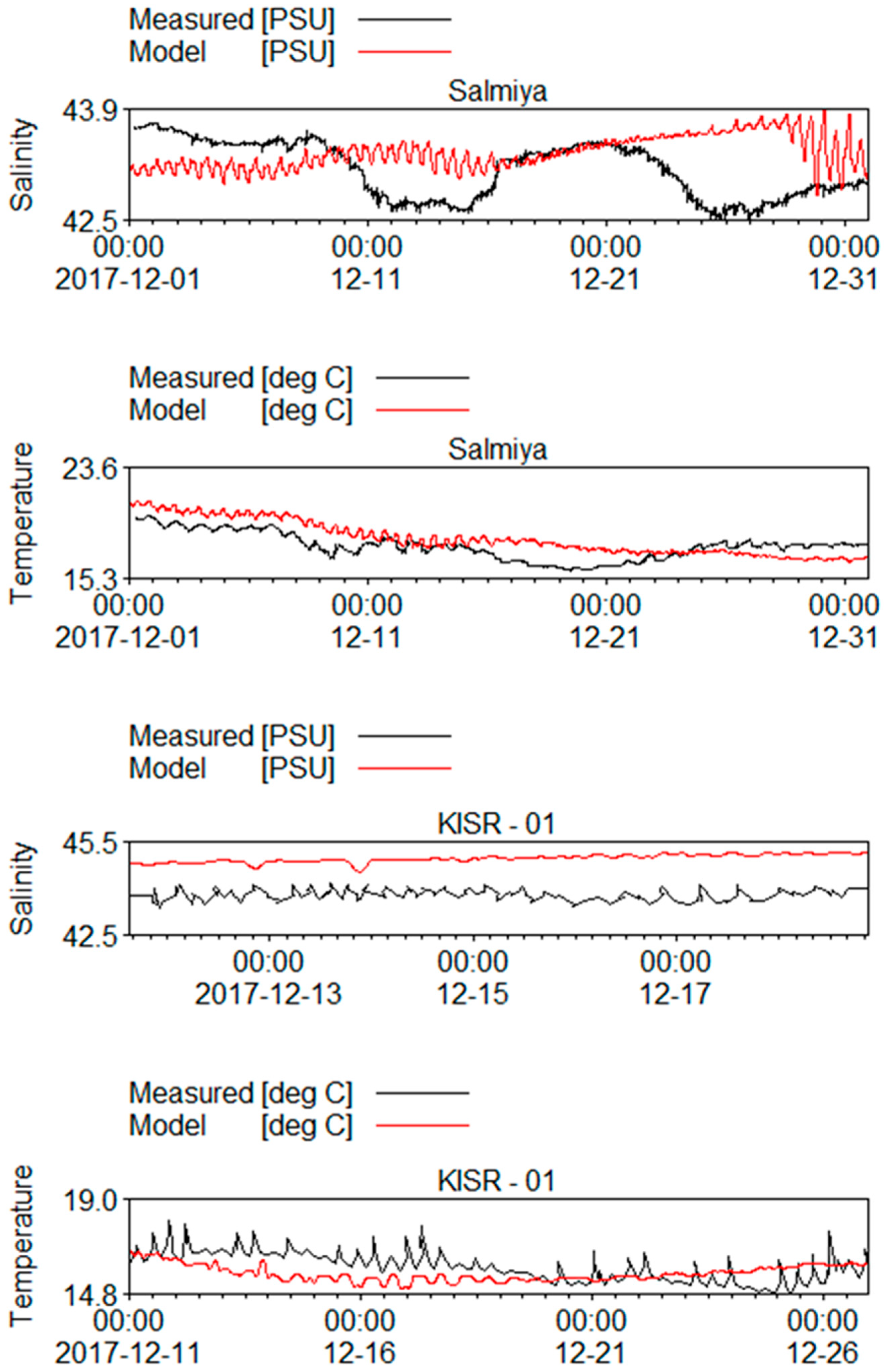
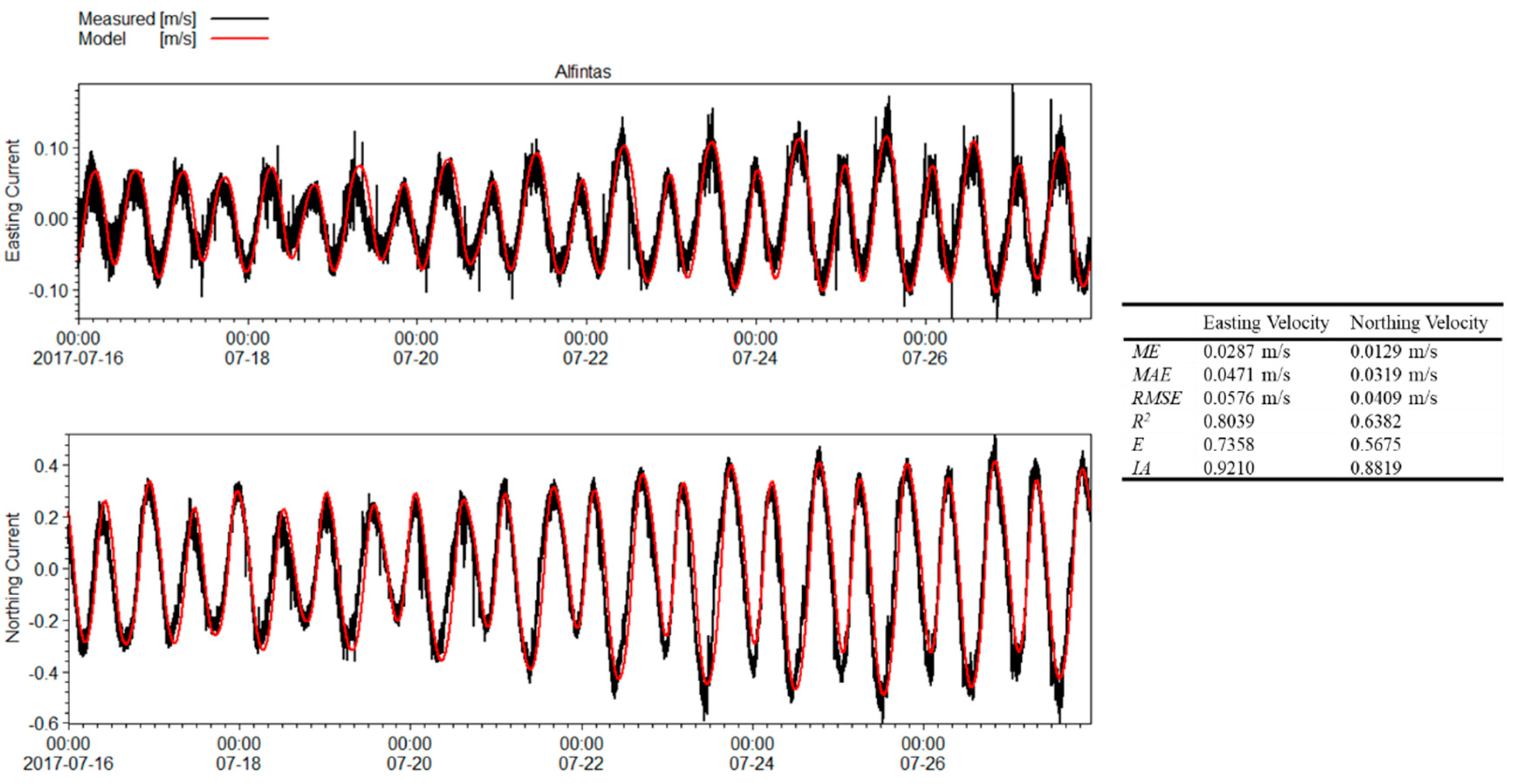
4.2. KHDM Validation

The KHDM has shown excellent predictive capabilities for water levels across various locations within the model domain, as evidenced in Figure 7 and Table 7. The model’s performance was evaluated using key metrics such as mean error (ME), mean absolute error (MAE), root mean square error (RMSE), coefficient of determination (R2), Nash–Sutcliffe coefficient (E), and the index of agreement (IA). When the last three parameters are closer to 1, there is a strong alignment between the model predictions and the actual measured data. Table 7 shows these parameters collectively, demonstrating a high level of accuracy in the model’s predictions of water levels.
For tidal currents, the KHDM accurately predicted conditions at the Alfintas station (Figure 8). The lower coefficients of determination (0.6382) and coefficient of efficiency (0.5675) are attributed to irregularities and sudden peaks in the data, which align with observations from previous studies in Kuwait and other locations [73,74,75]. Despite these variations, the KHDM effectively predicts water levels and tidal currents.
The hydrodynamic model’s calibration process required input parameter adjustments to enhance the accuracy of salinity and temperature predictions. The literature on coastal hydrodynamics acknowledges that such predictions frequently encounter variability due to the dynamic nature of coastal processes [76]. Studies within similar marine environments have noted that salinity and temperature predictions are susceptible to variations, particularly when affected by fluctuating boundary conditions and intermittent data collection [77,78,79].
Challenges were encountered when aligning model outcomes with measured data from the Salmiya and KISR-01 stations (Figure 9). Discrepancies primarily resulted from the absence of proximal salinity and temperature measurements during the simulation. Dependence on secondary data sources such as ERA5 and the Boundary Conditions Generator for MIKE 3 led to observable variations: salinity was overpredicted by an average of 1.23 PSU, while temperature was underpredicted by 2 °C. Despite these minor deviations, the model accurately captures the general patterns and trends of measured values consistent with known levels in the area [80,81].
The robustness of the model was evaluated against its predictive capacity for tidal levels and currents, which are crucial for such studies. The model demonstrated high precision in these critical aspects, as evidenced by the performance metrics in Table 7 and Figure 8.
In conclusion, despite the noted challenges, the model’s predictive accuracy for salinity and temperature remained within an acceptable range for the study’s purposes. A thorough calibration, supported by regional and related studies evidence, confirms the model’s reliability. The Kuwait hydrodynamic model (KHDM) is validated as a robust tool for developing advanced hydrodynamic and transport models, thereby contributing to a deeper understanding of marine dynamics, particularly in Kuwait’s coastal and marine environments.

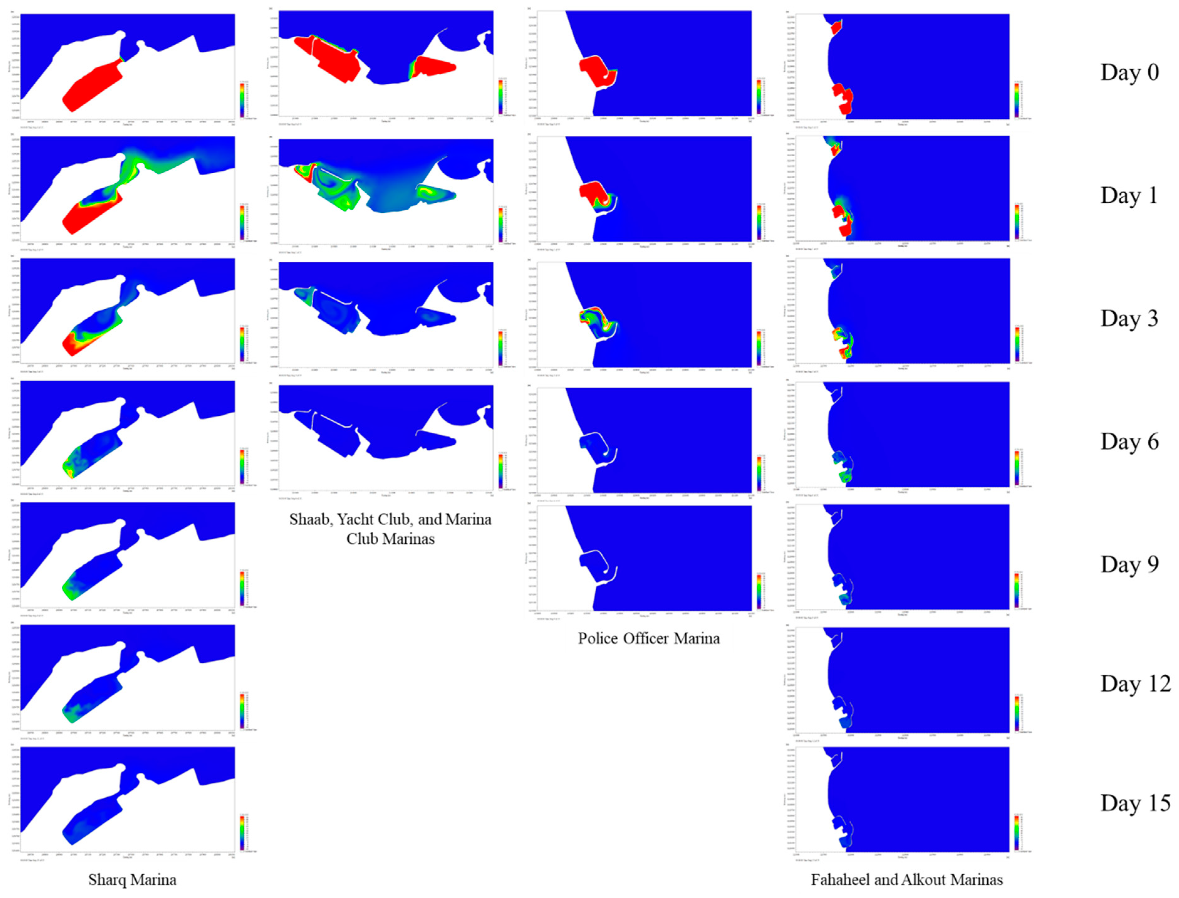
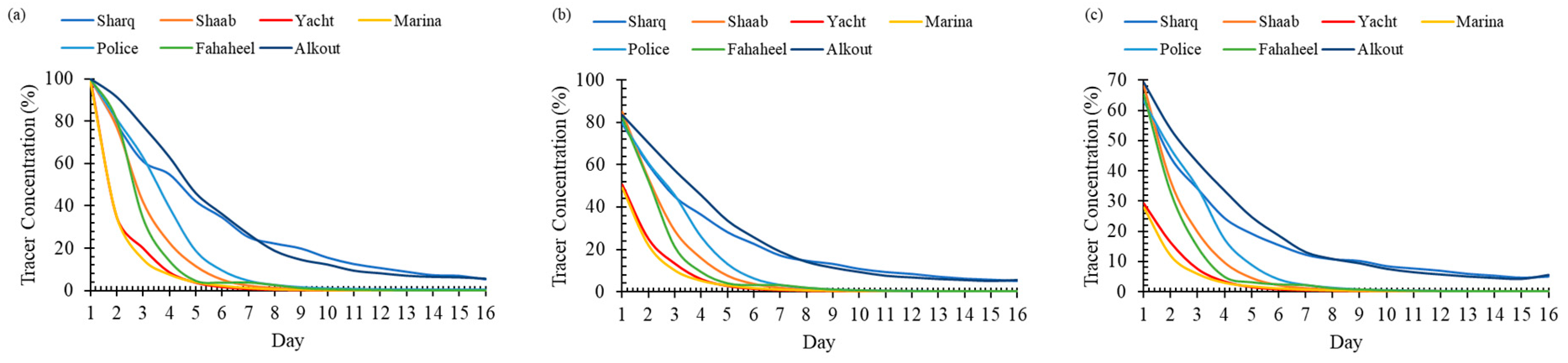
4.3. Transport Model and Flushing Capability
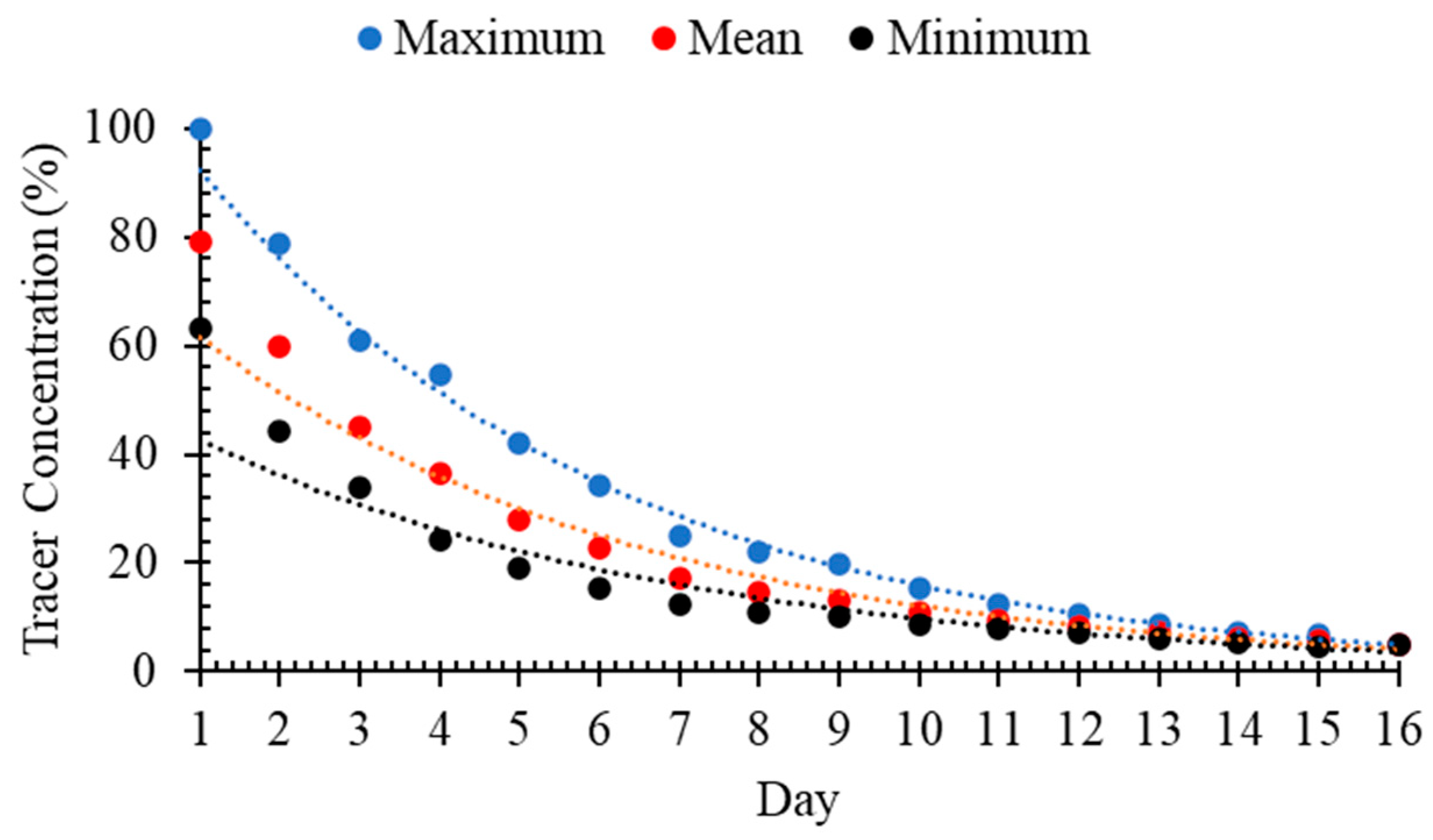
This study aimed to assess marinas’ water renewal factors and flushing capability by numerically assessing tracer concentration changes over tidal cycles. The findings from the transport model are presented in Table 8, and Figure 10 and Figure 11, which depict the daily maximum, mean, and minimum tracer concentrations.

Flushing Efficiency

In the Sharq, Police Officer, and Alkout Marinas, tracer average concentrations after three days were recorded between 44.9% and 57.2%, with peaks ranging from 61% to 77.7%. In contrast, other marinas experienced a rapid decrease in the mean concentrations, dropping below 30% after three days. After six days, Shaab, Yacht Club, Marina Club, Police Officer, and Fahaheel Marinas recorded a significant reduction in maximum mean tracer levels, reaching only 6.3%. Meanwhile, Sharq and Alkout Marinas maintained higher levels, with averages above 22.6% and peaks exceeding 34%. After 16 days, only Alkout and Sharq Marinas continued to show tracer concentrations above 5%, as levels in the remaining marinas neared zero. These results highlight the varied tracer concentration across different marinas, indicating hydrodynamic, geometric, environmental, and operational impacts.
Hence, Alkout and Sharq Marinas showed the least efficient water renewal. Factors such as their complex layout and entrance configuration, which protect from strong waves but hinder flushing efficiency, contribute to this. For instance, the meandering entrances create eddies and dead zones, obstructing water mixing [20]. Sharq Marina faces additional challenges due to its location behind Souq Sharq Mall and its shallow entrance orientation, which recesses about 2 km during low spring tide. Alkout Marina’s main issue was the presence of sheltered areas that do not face the open sea.
In contrast, Yacht Club and Marina Club Marinas exhibited more efficient flushing due to their simpler layouts and wider entrances. Both marinas showed excellent flushing capabilities within two days, with mean and maximum tracer concentrations less than 13.1% and 20.1%, respectively. Additionally, Yacht Club Marina benefits from a secondary 23-meter opening that enhances water circulation [9,19]. The smallest and second-smallest marinas, Alshaab and Fahaheel Clubs, demonstrated similar water renewal trends. However, Fahaheel Club Marina slightly outperformed Alshaab Marina due to its wider entrance and faster tidal currents outside Kuwait Bay.
Table 8, and Figure 10 and Figure 11, as well as the marina characteristics in Table 6, show that surface areas, layout configurations, locations, and hydrodynamic conditions are crucial in determining flushing efficiency. The observed decay in tracer concentration inside the marinas (Figure 11) aligns with the literature [10,18,39,48,50,82] and follows an exponential decay model as follows:
C % = a e b t f
Regression analysis fitted the data in Table 8 to Equation (21), yielding coefficients a and b, which reflect the maximum, average, and minimum daily concentration (Table 9). Figure 12 illustrates the model’s performance in predicting tracer concentration inside Sharq Marina. The model shows high accuracy, with a minimum R2 of 0.964 at the Fahaheel Club Marina and a maximum of 0.996 at the Yacht Club Marina. By correlating the hydrodynamics and geometry of the marinas with the empirical model (Equation (21)), a relationship was established encompassing most of the following factors determining flushing efficiency: the tidal prism, water level range, mean tidal currents, and average flow discharge at the channel entrance (Table 10) are related to the marina’s geometry and hydrodynamics. The regression analysis revealed that as the tidal prism and its ratio to the average discharge (P/Q) increase, the coefficients a and b decrease, as shown in Figure 13 and Equations (22) and (23). Equation (24), derived from substituting Equations (22) and (23) into Equation (21), is a general model to estimate the tracer concentration inside marinas for a given tidal prism, discharge ratio, and flushing time. With R2 values of 0.815 and 0.630 for Equations (22) and (23), respectively, this model is valuable for assessing the flushing efficiency of marinas and a preliminary estimation of flushing time in pollution incidents, selecting locations for new marinas, and optimizing the layouts of existing marinas. In Equation (24), P is in m3, Q is in m3/day, and tf is in days.
a = 1070 P 0.187
b = 0.1323 P Q 0.838
C % = 1070 P 0.187 e 0.1323 P Q 0.838 t f

5. Findings and Conclusions

Maintaining healthy marinas in terms of acceptable water quality is challenging and requires optimized design, proper management, and community awareness. The results of this study are instrumental in guiding marinas’ sustainable planning, development, and management.
Understanding flushing dynamics is crucial to maintaining or designing existing marinas. The marinas failed to meet established water quality standards due to inefficient flushing and inadequate environmental management. Notably, even in the absence of official sewage discharge sources, poorly flushed marinas exhibited significant pollution. This pollution is closely linked to each marina’s hydrodynamic and geometric characteristics, as reflected in the variability of parameters like BOD, COD, BOD/COD, DO, and SO42− levels.
Although the tracer concentration in all marinas decayed exponentially with time, the decay rate differed across marinas due to their unique hydrodynamic and geometric properties. The decay rate is expressed by the generalized exponential equation (Equation (24)), which is influenced by the tidal prism (P), the ratio of the tidal prism to mean flow discharge (P/Q), and flushing time (tf). This equation emerges as a critical tool for assessing marina flushing capabilities and aids in selecting sites and layouts for new marinas and optimizing existing layouts.
Design optimization has never been a unique solution to keep marinas clean and safe. A robust environmental management plan and community awareness are essential. The plan should include at least the following:
  • Monitoring and Regulation: Enhance the monitoring and regulation of pollutants contributing to water and sediment quality degradation, such as high BOD and COD and low DO levels.
  • Numerical Modeling: The numerical model’s accurate prediction of water levels and tidal currents underscores the significance of precise hydrodynamic modeling in managing marina environments and flushing characteristics.
  • Design Guidelines: Implement advanced design solutions like engineering-with-nature systems and slotted vertical and sloped structures to enhance water circulation, reduce stagnation, and promote natural pollutant cleansing. Incorporating nature-based solutions into marina management and design offers a promising avenue toward achieving sustainability.
  • Community Engagement: Encourage marina users and local communities to participate in sustainable practices and understand their impact on environmental health.
  • Policy and Regulation: Advocate for stricter environmental regulations and standards for marinas, ensuring accountability for maintaining water quality.
In conclusion, achieving sustainable marina development is a complex task that requires a harmonious combination of rigorous scientific research, innovative design, strict policy formulation, and active community involvement. This study highlights the importance of collaborative efforts among scientists, designers, marina authorities, environmental agencies, and the wider community in promoting the sustainability of coastal marinas. Adopting a comprehensive environmental management plan that addresses the numerous challenges marinas face is a significant opportunity to improve the quality of these vital coastal environments. Such concerted actions promise to protect the health and sustainability of marinas for future generations while preserving their natural beauty and biodiversity. Moving forward, this synergistic approach will be crucial in achieving the dual goals of marina sustainability and the preservation of ecological integrity, ensuring that marinas continue to thrive as bastions of beauty and biodiversity despite evolving environmental challenges.

Author Contributions

Conceptualization, M.A. and A.A.; methodology, M.A. and A.A.; software, M.A.; validation, M.A. and A.A.; formal analysis, M.A. and A.A.; investigation, M.A. and A.A.; resources, M.A.; data curation, M.A.; writing—original draft preparation, M.A. and A.A.; writing—review and editing, M.A. and A.A.; visualization, M.A.; supervision, M.A. and A.A.; project administration, M.A.; funding acquisition, M.A. All authors have read and agreed to the published version of the manuscript.

Funding

This research was funded by Kuwait University, grant number EV01/19.

Institutional Review Board Statement

Not applicable.

Informed Consent Statement

Not applicable.

Data Availability Statement

The data presented in this study are available on request from the corresponding author due to legal reasons.

Conflicts of Interest

The authors declare no conflicts of interest.

Appendix A

Table A1. Monthly DO concentrations and salinity levels at different marinas from May to October.
Marina MonthMonth
56789105678910
DO (mg/L)Salinity
SharqMinimum1.071.542.623.124.004.1340.9740.9942.2543.2442.4441.04
Average1.742.103.513.644.525.1140.9841.0642.3743.3443.3741.70
Maximum2.052.814.244.145.186.6140.9941.1342.6343.3743.8042.60
Sha’abMinimum2.903.024.071.102.753.7642.7040.1740.8340.9140.3140.06
Average3.893.644.782.664.024.7942.7840.3941.0841.9640.7640.55
Maximum4.674.235.724.954.745.4142.8540.4741.1942.8941.1740.91
Yacht ClubMinimum2.792.862.952.442.454.5243.0940.0440.3442.4941.8741.15
Average3.543.144.153.284.285.5543.1340.2641.0742.5742.2641.58
Maximum4.383.365.214.005.756.4243.1940.4641.2942.6642.7841.93
Marina ClubMinimum2.722.513.172.004.075.1539.8039.7541.0041.0040.6240.13
Average4.103.053.862.364.455.5240.6740.2941.3041.8341.7740.74
Maximum5.223.444.643.035.376.1342.4840.4941.3842.7042.2741.54
Fahaheel ClubMinimum1.261.894.102.751.462.7642.5739.9840.2640.3040.8040.34
Average2.402.434.333.632.063.9943.1140.1140.4341.6841.5140.62
Maximum2.952.934.664.882.555.7343.3540.2140.6342.8042.2940.87
AlkoutMinimum1.900.742.171.371.370.8540.2239.2939.9840.2940.1640.09
Average2.431.532.852.042.831.3941.2240.0040.4640.8540.8240.71
Maximum2.802.003.453.703.941.7842.7640.2540.6041.5141.4641.16
Table A2. Monthly Tw and pH levels at different marinas from May to October.
Marina MonthMonth
56789105678910
Tw (°C)pH
SharqMinimum29.8031.4031.2032.7031.3019.808.148.128.448.408.278.28
Average30.1331.6331.4832.8632.0926.018.188.208.488.458.438.47
Maximum30.3031.8031.7033.1036.6032.208.218.268.528.488.498.54
Sha’abMinimum28.5031.0029.1032.2024.7024.808.298.298.407.798.468.49
Average28.5831.2529.4032.3930.4326.408.308.318.438.308.498.51
Maximum28.7031.5029.7032.5035.4027.908.318.328.458.408.518.52
Yacht ClubMinimum28.5030.9028.9032.5026.3022.508.308.278.358.438.448.49
Average28.5631.2629.2932.5332.6126.258.328.318.418.458.488.51
Maximum28.6031.6029.6032.6038.1030.808.338.338.458.468.518.54
Marina ClubMinimum23.7031.0030.2032.3021.7024.808.248.258.398.328.238.29
Average25.4532.1630.3132.6127.9327.948.318.298.418.408.458.43
Maximum28.3033.2030.4033.1035.7030.508.348.338.448.478.528.49
Fahaheel ClubMinimum26.2031.3029.5030.3026.5022.808.168.208.428.338.398.46
Average26.5031.5329.5235.8030.7327.808.238.228.438.408.438.49
Maximum27.0032.0029.6038.1037.5032.008.268.238.448.458.468.52
AlkoutMinimum26.2031.6029.5031.1024.8021.208.188.098.298.238.088.23
Average26.6432.0629.6033.8434.0027.078.218.148.338.288.348.32
Maximum27.1032.9029.8036.0039.2031.708.248.208.388.338.408.40

References

  1. Davenport, J.; Davenport, J.L. The impact of tourism and personal leisure transport on coastal environments: A review. Estuar. Coast. Shelf Sci. 2006, 67, 280–292. [Google Scholar] [CrossRef]
  2. Valdor, P.F.; Gómez, A.G.; Juanes, J.A.; Kerléguer, C.; Steinberg, P.; Tanner, E.; MacLeod, C.; Knights, A.M.; Seitz, R.D.; Airoldi, L.; et al. A global atlas of the environmental risk of marinas on water quality. Mar. Pollut. Bull. 2019, 149, 110661. [Google Scholar] [CrossRef]
  3. Widmer, W.M.; Underwood, A.J. Factors affecting traffic and anchoring patterns of recreational boats in Sydney Harbour, Australia. Landsc. Urban Plan. 2004, 66, 173–183. [Google Scholar] [CrossRef]
  4. Association of Marina Industries. U.S. Marina Industry Economic Impact Study; Association of Marina Industries: Warren, RI, USA, 2018; p. 9. [Google Scholar]
  5. Crain, C.M.; Halpern, B.S.; Beck, M.W.; Kappel, C.V. Understanding and managing human threats to the coastal marine environment. Ann. N. Y. Acad. Sci. 2009, 1162, 39–62. [Google Scholar] [CrossRef] [PubMed]
  6. Yılmaz, A.; Karacık, B.; Henkelmann, B.; Pfister, G.; Schramm, K.W.; Yakan, S.D.; Barlas, B.; Okay, O.S. Use of passive samplers in pollution monitoring: A numerical approach for marinas. Environ. Int. 2014, 73, 85–93. [Google Scholar] [CrossRef]
  7. Tetra Tech. National Management Measures to Control Nonpoint Source Pollution from Marinas and Recreational Boating; Tetra Tech: Fairfax, VA, USA, 2000; p. 212. [Google Scholar]
  8. EPA. National Management Measures Guidance to Control Nonpoint Source Pollution from Marinas and Recreational Boating; United States Environmental Protection Agency: Washington, DC, USA, 2001.
  9. Flory, J.; Alber, M. Marinas: Best Management Practices & Water Quality: Prepared for GA DNR—Coastal Resources Division; Georgia Coastal Research Council: Athens, GA, USA, 2005. [Google Scholar]
  10. Nece, R.E.; Welch, E.B.; Reed, J.R. Flushing Criteria for Salt Water Marinas; University of Washington, Department of Civil and Environmental Engineering: Seattle, WA, USA, 1975. [Google Scholar]
  11. Petrosillo, I.; Valente, D.; Zaccarelli, N.; Zurlini, G. Managing tourist harbors: Are managers aware of the real environmental risks? Mar. Pollut. Bull. 2009, 58, 1454–1461. [Google Scholar] [CrossRef] [PubMed]
  12. Dolgen, D.; Alpaslan, M.N.; Serifoglu, A.G. Best waste management programs (BWMPs) for marinas: A case study. J. Coast. Conserv. 2003, 9, 57–63. [Google Scholar] [CrossRef]
  13. Alkhalidi, M.A.; Al-Nasser, Z.H.; Al-Sarawi, H.A. Environmental Impact of Sewage Discharge on Shallow Embayment and Mapping of Microbial Indicators. Front. Environ. Sci. 2022, 10, 914011. [Google Scholar] [CrossRef]
  14. Alkhalidi, M.; Alsulaili, A.; Almarshed, B.; Bouresly, M.; Alshawish, S. Assessment of Seasonal and Spatial Variations of Coastal Water Quality Using Multivariate Statistical Techniques. J. Mar. Sci. Eng. 2021, 9, 1292. [Google Scholar] [CrossRef]
  15. Almarshed, B.; Figlus, J.; Miller, J.; Verhagen, H.J. Innovative Coastal Risk Reduction through Hybrid Design: Combining Sand Cover and Structural Defenses. J. Coast. Res. 2019, 36, 174–188. [Google Scholar] [CrossRef]
  16. Alkhalidi, M.; Alanjari, N.; Neelamani, S. Wave Interaction with Single and Twin Vertical and Sloped Slotted Walls. J. Mar. Sci. Eng. 2020, 8, 589. [Google Scholar] [CrossRef]
  17. Alkhalidi, M.; Neelamani, S.; Al Haj Assad, A.I. Wave Forces and Dynamic Pressures on Slotted Vertical Wave Barriers with an Impermeable Wall in Random Wave Fields. Ocean Eng. 2015, 109, 1–6. [Google Scholar] [CrossRef]
  18. Gómez, A.G.; Ondiviela, B.; Fernández, M.; Juanes, J.A. Atlas of Susceptibility to Pollution in Marinas. Application to the Spanish Coast. Mar. Pollut. Bull. 2017, 114, 239–246. [Google Scholar] [CrossRef] [PubMed]
  19. Al-Khalidi, M.A.; Tayfun, M.A.; Al-Mershed, A.B. Tidal Recirculation of a Marina: A Case Study in Kuwait Bay. Kuwait J. Sci. Eng. 2011, 38, 1–17. [Google Scholar]
  20. Klein, R. The Effects of Marinas & Boating Activity upon Tidal Waterways; Community & Environmental Defense Services: Owings Mills, MD, USA, 2007. [Google Scholar]
  21. Kuwait Environment Public Authority (KEPA). Environmental Protection Law; Kuwait Environment Public Authority: Shuwaikh Industrial, Kuwait, 2014; Volume 42, p. 164.
  22. Wang, W.; Chang, J.-S.; Show, K.-Y.; Lee, D.-J. Anaerobic recalcitrance in wastewater treatment: A review. Bioresour. Technol. 2022, 363, 127920. [Google Scholar] [CrossRef] [PubMed]
  23. Dinçer, A.R. Increasing BOD5/COD ratio of non-biodegradable compound (reactive black 5) with ozone and catalase enzyme combination. SN Appl. Sci. 2020, 2, 736. [Google Scholar] [CrossRef]
  24. Alkhalidi, M.A.; Hasan, S.M.; Almarshed, B.F. Assessing Coastal Outfall Impact on Shallow Enclosed Bays Water Quality: Field and Statistical Analysis. J. Eng. Res. 2023, in press. [Google Scholar] [CrossRef]
  25. Daud, Z.; Awang, H.; Latif, A.A.A.; Nasir, N.; Ridzuan, M.B.; Ahmad, Z. Suspended Solid, Color, COD and Oil and Grease Removal from Biodiesel Wastewater by Coagulation and Flocculation Processes. Procedia—Soc. Behav. Sci. 2015, 195, 2407–2411. [Google Scholar] [CrossRef]
  26. Adjovu, G.E.; Stephen, H.; James, D.; Ahmad, S. Measurement of Total Dissolved Solids and Total Suspended Solids in Water Systems: A Review of the Issues, Conventional, and Remote Sensing Techniques. Remote Sens. 2023, 15, 3534. [Google Scholar] [CrossRef]
  27. Wang, H.; Zhang, Q. Research Advances in Identifying Sulfate Contamination Sources of Water Environment by Using Stable Isotopes. Int. J. Environ. Res. Public Health 2019, 16, 1914. [Google Scholar] [CrossRef]
  28. Geurts, J.J.M.; Sarneel, J.M.; Willers, B.J.C.; Roelofs, J.G.M.; Verhoeven, J.T.A.; Lamers, L.P.M. Interacting Effects of Sulphate Pollution, Sulphide Toxicity and Eutrophication on Vegetation Development in Fens: A Mesocosm Experiment. Environ. Pollut. 2009, 157, 2072–2081. [Google Scholar] [CrossRef] [PubMed]
  29. Tostevin, R.; Turchyn, A.V.; Farquhar, J.; Johnston, D.T.; Eldridge, D.L.; Bishop, J.K.B.; McIlvin, M. Multiple sulfur isotope constraints on the modern sulfur cycle. Earth Planet. Sci. Lett. 2014, 396, 14–21. [Google Scholar] [CrossRef]
  30. Li, X.; Liu, Y.; Zhou, A.; Zhang, B. Sulfur and oxygen isotope compositions of dissolved sulfate in the Yangtze River during high water period and its sulfate source tracing. Earth Sci. J. China Univ. Geosci. 2014, 39, 1648–1654. [Google Scholar]
  31. Torres-Martínez, J.A.; Mora, A.; Mahlknecht, J.; Kaown, D.; Barceló, D. Determining nitrate and sulfate pollution sources and transformations in a coastal aquifer impacted by seawater intrusion—A multi-isotopic approach combined with self-organizing maps and a Bayesian mixing model. J. Hazard. Mater. 2021, 417, 126103. [Google Scholar] [CrossRef] [PubMed]
  32. Schwartz, R.; Imberger, J. Flushing Behaviour of a Coastal Marina. In Coastal Engineering; American Society of Civil Engineers: Reston, VA, USA, 1989; pp. 2626–2640. [Google Scholar]
  33. Shen, J.; Haas, L. Calculating age and residence time in the tidal York River using three-dimensional model experiments. Estuar. Coast. Shelf Sci. 2004, 61, 449–461. [Google Scholar] [CrossRef]
  34. Abdelrhman, M.A. Simplified Modeling of Flushing and Residence Times in 42 Embayments in New England, USA, with Special Attention to Greenwich Bay, Rhode Island. Estuar. Coast. Shelf Sci. 2005, 62, 339–351. [Google Scholar] [CrossRef]
  35. DiLorenzo, J.L.; Ram, R.; Huang, P.; Najarian, T.O. Simplified Tidal-Flushing Model for Small Marinas. In Proceedings of the World Marina’91, Long Beach, CA, USA, 4–8 September 1991; pp. 402–411. [Google Scholar]
  36. EPA. Coastal Marinas Assessment Handbook; The Region I. V.—Atlanta, GA: Atlanta, GA, USA, 1985. [Google Scholar]
  37. Coastal Systems International. Water Quality at Marinas: Flushing; Coastal Systems International: Coral Gables, FL, USA, 2004; p. 4. [Google Scholar]
  38. Sámano, M.L.; Bárcena, J.F.; García, A.; Gómez, A.G.; Álvarez, C.; Revilla, J.A. Flushing Time as a Descriptor for Heavily Modified Water Bodies Classification and Management: Application to the Huelva Harbour. J. Environ. Manag. 2012, 107, 37–44. [Google Scholar] [CrossRef] [PubMed]
  39. Yin, J.; Falconer, R.A.; Pipilis, K.; Stamou, A.I. Flow Characteristics and Flushing Processes in Marinas and Coastal Embayments. WIT Trans. Built Environ. 1998, 36, 1–12. [Google Scholar]
  40. Barber, R.; Wearing, M. A simplified model for predicting the pollution exchange coefficient of small tidal embayments. Water Air Soil Pollut. Focus 2004, 4, 87–100. [Google Scholar] [CrossRef]
  41. Nece, R.E.; Richey, E.P. Flushing Characteristics of Small-Boat Marinas. In Proceedings of the 13th Conference on Coastal Engineering, Vancouver, BC, Canada, 29 January 1972; pp. 2499–2512. [Google Scholar]
  42. Nece, R.E. Planform Effects on Tidal Flushing of Marinas. J. Waterw. Port Coast. Ocean Eng. 1984, 110, 251–269. [Google Scholar] [CrossRef]
  43. EPA. Coastal Marina Assessment Handbook; Environmental Protection Agency: Atlanta, GA, USA, 1985; p. 610. [Google Scholar]
  44. Sanford Lawrence, P.; Boicourt William, C.; Rives Stephen, R. Model for Estimating Tidal Flushing of Small Embayments. J. Waterw. Port Coast. Ocean Eng. 1992, 118, 635–654. [Google Scholar] [CrossRef]
  45. Edwards, A.; Sharples, F. Scottish Sea Lochs: A Catalogue; Scottish Marine Biological Association: Oban, UK, 1986. [Google Scholar]
  46. Hartnett, M.; Gleeson, F.; Falconer, R.; Finegan, M. Flushing Study Assessment of a Tidally Active Coastal Embayment. Adv. Environ. Res. 2003, 7, 847–857. [Google Scholar] [CrossRef]
  47. Fischer, H.B.; List, J.E.; Koh, C.R.; Imberger, J.; Brooks, N.H. Mixing in Inland and Coastal Waters; Academic Press: Cambridge, MA, USA, 1979. [Google Scholar]
  48. Monsen, N.E.; Cloern, J.E.; Lucas, L.V.; Monismith, S.G. A Comment on the Use of Flushing Time, Residence Time, and Age as Transport Time Scales. Limnol. Oceanogr. 2002, 47, 1545–1553. [Google Scholar] [CrossRef]
  49. Dyer, K.R. Estuaries: A Physical Introduction, 2nd ed.; John Wiley and Sons: Chichester, UK, 1997; p. 195. [Google Scholar]
  50. Thomann, R.V.; Mueller, J.A. Principles of Surface Water Quality Modeling and Control; Harper-Collins: New York, NY, USA, 1987; p. 644. [Google Scholar]
  51. Gómez, A.G.; Juanes, J.A.; Ondiviela, B.; Revilla, J.A. Assessment of Susceptibility to Pollution in Littoral Waters using the Concept of Recovery Time. Mar. Pollut. Bull. 2014, 81, 140–148. [Google Scholar] [CrossRef] [PubMed]
  52. Lebleb, A.; Galal, E.; Tolba, E. A Hydrodynamic Study of Water Flushing Parameters to Improve the Water Quality Inside Marinas and Lagoons. Port-Said Eng. Res. J. 2020, 24, 52–62. [Google Scholar] [CrossRef]
  53. Environment Protection Authority. Approved Methods for the Sampling and Analysis of Water Pollutants in NSW; NSW Environment Protection Authority: Parramatta, Australia, 2022; p. 55. [Google Scholar]
  54. American Public Health Association (APHA); American Water Works Association (AWWA); Water Environment Federation (WEF). Standard Methods for the Examination of the Water and Wastewater, 23rd ed.; Beird, R.B., Eaton, A.D., Rice, E.W., Eds.; APHA: Washington, DC, USA; AWWA: Washington, DC, USA; WEF: Washington, DC, USA, 2017. [Google Scholar]
  55. DHI. MIKE 3 Flow Model FM, Hydrodynamic and Transport Module, Scientific Documentation; Danish Hydraulic Institute: Hørsholm, Denmark, 2024. [Google Scholar]
  56. DHI. MIKE 3 Flow Model FM: Hydrodynamic Module User Guide; Danish Hydraulic Institute: Hørsholm, Denmark, 2024. [Google Scholar]
  57. Alsulaiman, N. Three-Dimensional Hydrodynamic Modelling of the Wintertime Variation of Kuwait Bay; Kuwait University: Kuwait City, Kuwait, 2019. [Google Scholar]
  58. DHI. MIKE C-MAP: Extraction of World Wide Bathymetry Data and Tidal Information User Guide; Danish Hydraulic Institute: Hørsholm, Denmark, 2019; p. 42. [Google Scholar]
  59. DHI. Boundary Conditions Generator for MIKE 3. Available online: https://www.dhigroup.com/marine-water/boundary-conditions-generator (accessed on 21 August 2022).
  60. Dee, D.P.; Uppala, S.M.; Simmons, A.J.; Berrisford, P.; Poli, P.; Kobayashi, S.; Andrae, U.; Balmaseda, M.A.; Balsamo, G.; Bauer, P.; et al. The Era-Interim Reanalysis: Configuration and Performance of the Data Assimilation System. Q. J. R. Meteorol. Soc. 2011, 137, 553–597. [Google Scholar] [CrossRef]
  61. Wilcox, D.C. Basic Fluid Mechanics; DCW Industries: La Cañada, CA, USA, 2000. [Google Scholar]
  62. US Army Corps of Engineers. Engineering and Design Environmental Engineering for Small Boat Basins; EM 1110-2-1206; US Army Corps of Engineers: Washington, DC, USA, 1993. [Google Scholar]
  63. Moran, S. Chapter 6—Clean water characterization and treatment objectives. In An Applied Guide to Water and Effluent Treatment Plant Design; Moran, S., Ed.; Butterworth-Heinemann: Oxford, UK, 2018; pp. 61–67. [Google Scholar]
  64. Central Statistical Bureau. Annual Statistical Abstract; Central Statistical Bureau: Kuwait City, Kuwai, 2018. [Google Scholar]
  65. Scully, M.E.; Geyer, W.R.; Borkman, D.; Pugh, T.L.; Costa, A.; Nichols, O.C. Unprecedented Summer Hypoxia in Southern Cape Cod Bay: An Ecological Response to Regional Climate Change? Biogeosciences 2022, 19, 3523–3536. [Google Scholar] [CrossRef]
  66. Diaz, R.J.; Breitburg, D.L. Chapter 1 The Hypoxic Environment. In Fish Physiology; Richards, J.G., Farrell, A.P., Brauner, C.J., Eds.; Academic Press: Cambridge, MA, USA, 2009; Volume 27, pp. 1–23. [Google Scholar]
  67. Liu, S.; Lou, S.; Kuang, C.; Huang, W.; Chen, W.; Zhang, J.; Zhong, G. Water Quality Assessment by Pollution-Index Method in the Coastal Waters of Hebei Province in Western Bohai Sea, China. Mar. Pollut. Bull. 2011, 62, 2220–2229. [Google Scholar] [CrossRef]
  68. EPA. Guidance Specifying Management Measures for Sources of Nonpoint Pollution in Coastal Waters; United States Environmental Protection Agency: Washington, DC, USA, 1993. [Google Scholar]
  69. San Francisco Regional Water Quality Control Board. California’s Vessel Sewage Guide. California State Parks Division of Boating and Waterways’ Clean Vessel Act Program. 2019. Available online: https://cms.santamonicabay.org/wp-content/uploads/2019/09/when-nature-calls_FINAL_2019_for-web.pdf (accessed on 10 March 2024).
  70. Milliken, A.S.; Lee, V. Pollution Impacts from Recreational Boating: A Bibliography and Summary Review. Rhode Island Sea Grant Number RIU-G-90-002 C4. 1990. Available online: https://repository.library.noaa.gov/view/noaa/11840/noaa_11840_DS1.pdf (accessed on 10 March 2024).
  71. Division of Environmental Management—Water Quality Section. North Carolina Coastal Marinas: Water Quality Assessment; 90-01; North Carolina Department of Environment, Health and Natural Resources: Raleigh, NC, USA, 1990. [Google Scholar]
  72. Koch, M.; Yediler, A.; Lienert, D.; Insel, G.; Kettrup, A. Ozonation of Hydrolyzed Azo Dye Reactive Yellow 84 (Ci). Chemosphere 2002, 46, 109–113. [Google Scholar] [CrossRef]
  73. Lafta, A.A.; Altaei, S.A.; Al-Hashimi, N.H. Impacts of Potential Sea-Level Rise on Tidal Dynamics in Khor Abdullah and Khor Al-Zubair, Northwest of Arabian Gulf. Earth Syst. Environ. 2020, 4, 93–105. [Google Scholar] [CrossRef]
  74. Al Mamoon, A.; Keupink, E.; Rahman, M.M.; Eljack, Z.A.; Rahman, A. Sea Outfall Disposal of Stormwater in Doha Bay: Risk Assessment Based on Dispersion Modelling. Sci. Total Environ. 2020, 732, 139305. [Google Scholar] [CrossRef] [PubMed]
  75. Alosairi, Y.; Pokavanich, T.; Alsulaiman, N. Three-Dimensional Hydrodynamic Modelling Study of Reverse Estuarine Circulation: Kuwait Bay. Mar. Pollut. Bull. 2018, 127, 82–96. [Google Scholar] [CrossRef] [PubMed]
  76. de Pablo, H.; Sobrinho, J.; Garcia, M.; Campuzano, F.; Juliano, M.; Neves, R. Validation of the 3D-MOHID Hydrodynamic Model for the Tagus Coastal Area. Water 2019, 11, 1713. [Google Scholar] [CrossRef]
  77. Lakhan, V.C.; Trenhaile, A.S. Chapter 1 Models and the Coastal System. In Elsevier Oceanography Series; Lakhan, V.C., Trenhaile, A.S., Eds.; Elsevier: Amsterdam, The Netherlands, 1989; Volume 49, pp. 1–16. [Google Scholar]
  78. Murthy, C.R.; Sinha, P.C.; Rao, Y. Modelling and Monitoring of Coastal Marine Processes; Springer: Berlin/Heidelberg, Germany, 2008. [Google Scholar]
  79. Wild-Allen, K.; Andrewartha, J. Connectivity between estuaries influences nutrient transport, cycling and water quality. Mar. Chem. 2016, 185, 12–26. [Google Scholar] [CrossRef]
  80. Al-Dousari, A.E. Desalination Leading to Salinity Variations in Kuwait Marine Waters. Am. J. Environ. Sci. 2009, 5, 451. [Google Scholar] [CrossRef]
  81. Al-Said, T.; Al-Ghunaim, A.; Subba Rao, D.V.; Al-Yamani, F.; Al-Rifaie, K.; Al-Baz, A. Salinity-driven decadal changes in phytoplankton community in the NW Arabian Gulf of Kuwait. Environ. Monit. Assess. 2017, 189, 268. [Google Scholar] [CrossRef]
  82. Patgaonkar, R.S.; Vethamony, P.; Lokesh, K.S.; Babu, M.T. Residence Time of Pollutants Discharged in the Gulf of Kachchh, Northwestern Arabian Sea. Mar. Pollut. Bull. 2012, 64, 1659–1666. [Google Scholar] [CrossRef]
Figure 1. The locations of tidal measurements and the marinas (Source: Google Earth Pro).
Jmse 12 00649 g001
Figure 2. Monthly maximum, minimum, and average: (a) TDS, (b) BOD, (c) COD, and (d) SO42− in all marinas.
Jmse 12 00649 g002
Figure 3. Monthly maximum, minimum, and average: BOD/COD.
Jmse 12 00649 g003
Figure 4. Flexible mesh of Kuwait before (left) and after (right) the bathymetric interpolation.
Jmse 12 00649 g004
Figure 5. Samples of the water level boundary conditions at the south (a) and east (b), the salinity (c), temperature (d), relative humidity (e), and air temperature (f) and wind rose (g) at (48.13333, 29.43333).
Jmse 12 00649 g005
Figure 6. Tracer concentration inside (red: 100%) and outside (blue: 0%) the marinas, at the beginning of each simulation.
Jmse 12 00649 g006
Figure 7. Measured versus model water levels at Failaka, KBay, Salmiya, and Alfintas stations.
Jmse 12 00649 g007
Figure 8. Measured versus model tidal currents at Alfintas station and the goodness of fit measures for tidal currents near Alfintas (Alfintas station).
Jmse 12 00649 g008
Figure 9. Measured versus model salinity and temperature at Salmiya and KISR-01 stations.
Jmse 12 00649 g009
Figure 10. Variation of the tracer concentration with time inside the marina’s basins.
Jmse 12 00649 g010
Figure 11. Variation of the daily (a) maximum, (b) mean, and (c) minimum tracer concentration inside all marinas.
Jmse 12 00649 g011
Figure 12. Comparison of daily modeled maximum, mean, and minimum tracer concentrations within Sharq Marina over a 16-day period against Equation (21) (dashed lines).
Jmse 12 00649 g012
Figure 13. Variation of the mean ‘a’ (left) and ‘b’ (right) coefficients of Equation (21) with the tidal prism (P) and the tidal prism to the average discharge through the inlet (P/Q) ratio, respectively.
Jmse 12 00649 g013
Table 1. Definition of the terms in Equations (12)–(18).
TermDefinition
t: Time
x, y, z: Cartesian coordinates
u, v, and w: Flow velocity components
S: Magnitude of discharge due to point sources
η : Surface elevation
d: Still water depth
h: Total   water   depth   ( η + d )
f :Coriolis parameter
g : G r a v i t a t i o n a l   a c c e l e r a t i o n
ρ : Density of water
ρ : Reference density
s y x , s x x , s y y , s x y : Radiation stress tensor components
V t : Vertical turbulence (or eddy) viscosity
P a : Atmospheric pressure
u s , v s : The velocity of discharged water from the source points to ambient water
F u , F v : Horizontal stress terms
T: Temperature
s: Salinity
Dv: Vertical turbulent (eddy) diffusion coefficient
H: Source term due to heat exchange with the atmosphere
Ts: Temperature of the source
ss: Salinity of the source
FT, Fs: Horizontal diffusion terms for temperature and salinity
Dh: Horizontal diffusion coefficient
Table 2. Minimum, maximum, and mean tidal ranges at the south and east boundaries.
LocationMinimum Neap Tidal Range (m)Maximum Spring Tidal Range (m)Mean Tidal Range (m)
South0.632.341.30
East0.852.931.73
Table 3. Model basic input parameters.
ParameterValueSource
Flooding and DryingDrying depth = 0.01Sensitivity analysis
Flooding depth = 0.05Default
Wetting depth = 0.1Default
Horizontal Eddy ViscositySmagorinsky coefficient = 0.4Sensitivity analysis
(0.25–1 [55])
Vertical Eddy ViscosityLog law formulation.Default
Bed ResistanceQuadratic drag coefficient = 0.01Default
Horizontal Dispersion (Salinity + Temperature)Dispersion coefficient formulation. Constant value: 15 m2/sSensitivity analysis
Vertical Dispersion (Salinity)Scaled eddy viscosity formulation. Scaling factor = 0.02Sensitivity analysis
Vertical Dispersion (Temperature)Scaled eddy viscosity formulation. Scaling factor = 0.08Sensitivity analysis
Table 4. The model source points’ locations and discharge properties [57].
Source PointLongitude, LatitudeDischarge
(m3/s)
Excess
Salinity (PSU)
Excess
Temperature (°C)
Doha East47.80399, 29.372583.50023.5
Doha West47.82137, 29.362208.71023.5
Shuwaikh47.94500, 29.357004.89423.5
AlSubiya47.70590, 29.359888.90623.5
Shuaiba48.15578, 29.03326 8.70023.5
Alzour48.379172, 28.698638.70023.5
Table 5. Simulation periods and tidal station location measurement information.
LocationSimulation PeriodMeasured Data PeriodData Type
1. KBay21 May 2012–16 July 201221 June 2012–16 July 2012Water level and temperature
2. Failaka10 November 2012–10 December 201210 November 2012–10 December 2012Water level
3. Salmiya1 November 2017–1 March 20181 December 2017–1 March 2018Water level, salinity, and temperature
4. KISR–011 November 2017–1 March 20181 December 2017–31 December 2017Salinity and temperature
5. Alfintas15 June 2017–29 July 201715 July 2017–29 July 2017Water level, tidal current, and direction
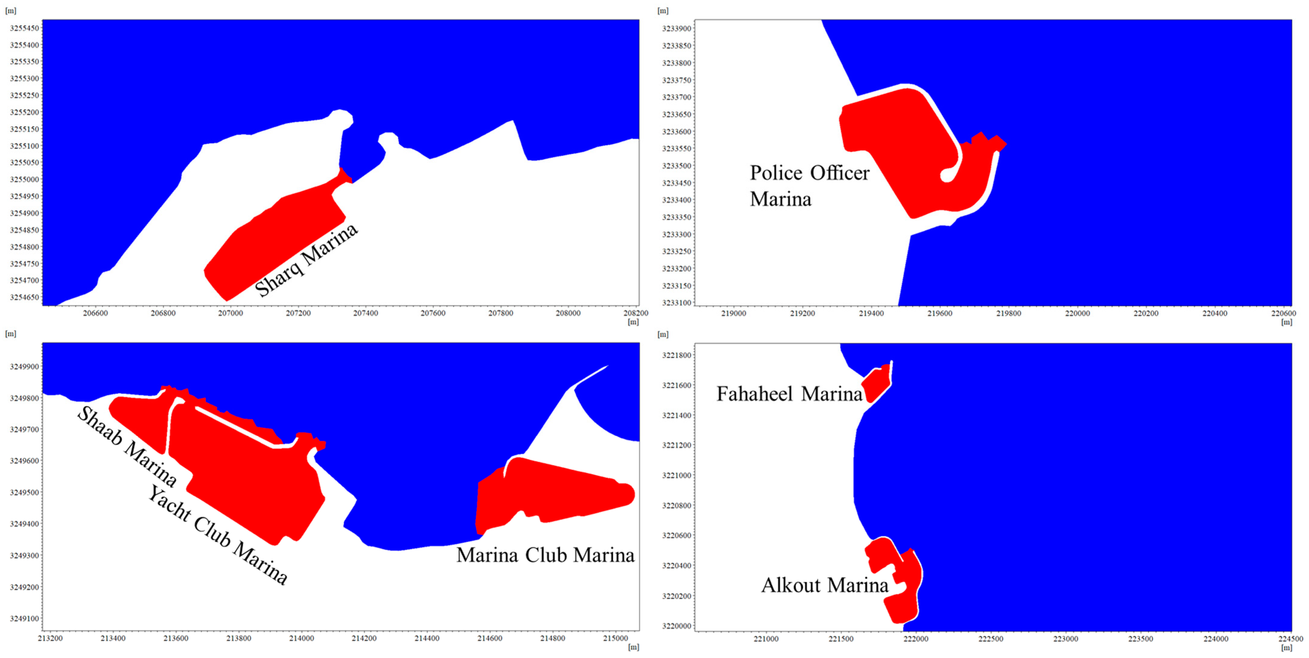
Table 6. Characteristics of the study marinas.
MarinaMaximum
Width
(m)
Maximum
Length
(m)
Surface
Area
(m2)
Entrance
Width
(m)
Depth
(m)
Spring Tidal
Range
(m)
Neap Tidal
Range
(m)
Sharq19043572,45628.5342.1
Sha’ab21217522,0993033.51.45
Yacht Club546334125,72223 and 5533.51.45
Marina Club19341156,02611033.51.45
Police Officer38027794,5808252.950.80
Fahaheel Club14521026,9975132.940.78
Alkout580317104,7268332.930.76
Table 7. The goodness of fit indices for water levels at KBay, Failaka, Salmiya, and Alfintas stations.
StationMEMAERMSER2EIA
KBay−0.1450.2190.2610.9460.9210.979
Failaka−0.0020.1120.1420.9640.9630.991
Salmiya0.0700.1410.1720.9540.9450.985
Alfintas−0.0660.0950.1170.9810.9720.993
Table 8. Daily maximum, minimum, and mean tracer concentration (%) at marinas.
Marina
SharqShaabYacht ClubMarina ClubPolice OfficerFahaheel ClubAlkout
DayMaxMeanMinMaxMeanMinMaxMeanMinMaxMeanMinMaxMeanMinMaxMeanMinMaxMeanMin
1100.079.363.3100.084.968.1100.050.529.110049.227.8100.080.262.8100.082.265.3100.083.369.1
278.659.944.377.253.336.334.824.816.134.921.811.880.960.847.180.752.232.891.470.153.6
361.044.934.041.928.619.520.113.17.414.89.95.862.945.634.234.221.014.677.757.242.6
454.836.424.322.715.79.58.75.83.37.65.12.939.225.917.214.19.24.863.045.533.2
542.128.119.211.67.44.53.82.51.54.02.81.718.713.18.94.73.93.146.033.524.6
634.422.615.55.23.52.11.71.20.72.31.51.09.46.34.13.83.02.436.025.618.5
725.117.112.32.41.71.10.80.60.41.20.80.64.53.22.33.93.02.126.618.913.0
822.114.710.81.31.00.60.40.40.30.60.50.32.51.81.42.71.81.118.614.010.8
919.713.210.30.70.50.40.30.20.20.40.30.21.41.10.81.20.90.714.411.39.3
1015.410.88.50.40.30.30.20.20.20.20.20.20.90.70.50.70.50.412.19.37.5
1112.49.37.80.30.20.20.20.10.10.20.20.10.60.50.40.40.30.39.37.56.4
1210.58.47.00.20.20.20.10.10.10.10.10.10.40.40.30.30.20.28.06.75.6
138.77.16.00.20.10.10.10.10.10.10.10.10.40.30.30.20.10.16.96.04.9
147.16.25.40.10.10.10.10.10.10.10.10.10.30.30.20.10.10.16.35.54.5
156.85.74.70.10.10.10.10.10.10.10.10.10.30.20.20.20.10.16.15.04.2
165.15.15.10.10.10.10.10.10.10.10.10.10.20.20.20.10.10.15.55.55.5
Table 9. Equation (21) coefficients for the marinas’ maximum, average, and minimum daily concentration.
Maximum Daily ConcentrationAverage Daily ConcentrationMinimum Daily Concentration
MarinaabR2abR2abR2
Sharq120.900.210.99796.110.230.99075.810.250.972
Shaab Club171.060.480.983151.050.560.997130.160.640.997
Yacht Club246.430.910.995102.260.711.00058.020.680.998
Marina Club260.430.970.998107.610.790.99961.160.800.998
Police Officer157.440.380.972127.450.410.982101.850.430.982
Fahaheel Club183.950.540.964159.490.630.989137.870.740.998
Alkout135.470.220.983109.270.240.99388.440.250.994
Table 10. Variations of Equation (24) coefficients with the marina’s geometry and the hydrodynamic conditions.
Marinaa
-
b
1/Day
Area
× 104 m2
Tidal
Range
m
Tidal Prism
× 104 m3
Q
× 104 m3/Day
P/Q
Day
Sharq96.110.237.092.2215.7726.470.60
Shaab151.050.562.212.034.4928.620.16
Yacht102.260.7012.572.0351.15173.420.15
Marina107.610.795.602.0311.3669.020.16
Police127.450.419.461.6615.6879.930.20
Fahaheel159.490.632.701.544.1717.440.24
Alkout109.270.2310.471.5416.0956.660.28
Disclaimer/Publisher’s Note: The statements, opinions and data contained in all publications are solely those of the individual author(s) and contributor(s) and not of MDPI and/or the editor(s). MDPI and/or the editor(s) disclaim responsibility for any injury to people or property resulting from any ideas, methods, instructions or products referred to in the content.

