Comparison of Different Methods for Ancient Ship Calm Water Resistance Estimation

Abstract

The remains of ancient ships from various time periods are commonly found on land and under the sea in conditions that make it difficult to reconstruct their original form and structure. For this reason, the reconstruction should be supported by other data, such as data on similar ships, but also by certain assumptions. The results of the reconstruction are significant not only in a historical sense but are of exceptional importance when building floating replicas. Two ships, Nin 1 and Nin 2, today for promotional purposes known as Condurae Croaticae, were found in Nin (Croatia) at the end of the 1960s. They are about 8 to 10 m long, and tentatively dated to the 11th century AD, although there are indications that they could be dated two centuries later. Based on archaeological finds exhibited in the Museum of Nin Antiquities, hull line drawings were created, according to which two floating replicas were made at the end of the 1990s. Considering the problem of hogging that appeared in both ships, a new proposal for the reconstruction of the original hull lines was performed based on the available documentation. The aim of this paper is a systematic analysis of its calm water resistance. Based on the established credibility of experimental testing, a scale model (1:4 ratio) of the Nin 1 vessel is constructed and evaluated through towing tank experiments. The second approach, the CFD method, is a reliable numerical method for calm resistance estimation, but it is rarely used in the analysis of ancient ships. Finally, the widely used empirical Holtrop method is also applied, but it was developed for ships of larger dimensions and with large parts of flat bottoms and, therefore, the more appropriate Delft Hull Yacht Series method is also tested. The results obtained by applying the four mentioned methods are compared and discussed.

1. Introduction

Reconstruction of the original forms of ancient vessels is a prevalent practice within nautical archaeology, as evidenced by numerous projects [1,2,3]. Conducting hydrodynamic analyses on these reconstructed ships requires a distinct set of engineering expertise and thrives within interdisciplinary collaborations. Understanding the sailing performance of ancient ships gives better insight into their capabilities and thus their purpose.

The most straightforward example of applying modern technologies for assessing old vessel hydrodynamic properties was completed by Murray et al. [4], where experimental towing tank tests were performed so the origin and development of the waterline ram could be investigated. By using towing tank testing, the authors supported their suspicion that bow projection was not just developed as an offensive weapon but also functioned as cutwater and thus, increased hull speed.

Because of the advancement of software packages, their capability of solving highly complex physical phenomena as well as the expansion of computational resources, numerical analysis started to be applied in nautical archaeology to estimate a wide range of ship sailing capabilities and detect various ship sailing characteristics. One such example was performed by Palmer [5], who modelled environmental loads and described the windward sailing capability of ancient vessels. Another study [6] implemented a Computational Fluid Dynamics (CFD) approach to assess a square-rigged sailing vessel, which was performed by using CFD software Fluent 6. 3 for calculating pressure. Exploration of ancient ship sailing capabilities under different wind incidence angles and yard angles was performed by Ciortan and Fonseca [7]. A more complex transient simulation of ship sinkage was performed by Rudan and Radić Rossi [8], but this time, an Arbitrary Lagrangian–Eulerian approach (ALE) was used. The goal of the study was to record the movement of both ship and cargo during ship capsizing. The whole simulation was divided into two phases including the first phase, where a simple ship model was exposed to side waves and its movement was analysed, while in the second phase, movements from the first phase were superimposed on a much more complex model consisting of modelled cargo. Another similar study of ship motion analysis was performed [9] by using the hypothetical model Barcode 02, the largest excavated ship in Oslo harbour. The study gave insight into ship performance on the sea and provided marine archaeologists with better insight into ship capabilities.

While the aforementioned studies are focused on assessing sailing under different environmental loads, there is a clear lack of thorough studies of ancient ship hydrodynamic properties, mainly ship resistance determination. The importance of accurate ship resistance calculation is crucial for both nautical archaeology and naval engineering, as it helps us understand how ancient vessels were designed and how they performed at sea. By carefully analysing each component of hydrodynamic resistance, i.e., wave and viscous components, nautical archaeologists together with engineers can piece together how fast and how far these ships could have travelled.

As already mentioned, numerical analysis is gaining popularity in nautical archaeology research, so numerous different software packages as well as methods are used for this purpose. A hydrodynamic study of the ideal wave pattern and frictional and wave-making resistance was conducted by Subbaiah et al. [10] for the traditional vessel Kerrala using Shipflow 5.1 software based on the Finite Volume Approach. Another possible approach to assessing ship hydrodynamic characteristics is the use of empirical methods. In one such study, Jerat et al. [11] examined uncertainty in the hull dimension and its impact on sailing characteristics. Ancient merchant ship Kyrenia with a hypothetical hull beam was considered, as well as its variations of ±5% and ±10%, leaving all other dimensions of the ship unchanged. A study conducted ship resistance calculation by using the empirical Holtrop–Mennen method. Handley [12] used the same empirical Holtrop–Mennen method, but this time, not for ship resistance calculation but instead for assessing probable ship displacement and, consequently, maximum cargo capacity. Using the Holtrop–Mennen method for detailed ship reconstruction, Tanner et al. [13] showed the need for a hydrodynamic calculation method that offers the possibility of predicting every ship scenario.

Prior studies have highlighted the critical role of hydrodynamic modelling in nautical archaeology, serving purposes such as evaluating stability concerns (e.g., capsizing and sinkage), assessing sailing performance, and determining optimal hull geometries based on propulsion capabilities. However, there has not been a detailed comparison of different methods to see how precise they are and if they are a good fit for calculating the resistance of ancient ships.

2. Aim and Scope of this Work

While ship resistance is a topic that has been extensively researched and presented over the last two decades, the analysis of ancient ship resistance with hull form differing from the modern hull is research in progress. Even though well-established procedures for resistance calculation already exist, each of them has its limitations and drawbacks, and they are not verified on hull forms that were not experimentally tested before that. In this article, four different methods for ship resistance calculation are applied and compared. With this study, verification of results gained by conventional empirical methods such as Holtrop–Mennen and Delft Yacht Hull series for non-conventional hulls are performed, and a comparison between experimental results is shown. The structure of this article is as follows:

• A detailed explanation of methods used for assessing (ancient) ship resistance on calm water is presented in Section 3 with a short description of the theoretical background for all four methods;
• Initial data, such as ship particulars (model size and life size), and materials and methods are stated for each method in Section 4 with an explanation of the chosen calculation parameters;
• Results are presented in Section 5 with a model size comparison between CFD and the experiment presented in Section 5.1 and a comparison of all four methods on a life-size ship presented in Section 5.2;
• The Discussion and Conclusion Section 6 and Section 7 focus on the findings obtained as well as pointing out the potential issues and/or limitations of the applied methods.

This approach was added to see how results differ when there is no applied extrapolation method and to investigate if an extrapolation method can result in a potentially bigger result difference. Regarding CFD analysis, an additional set of numerical calculations with surface roughness is presented to examine if the implementation of this phenomenon leads to better overlap with experimental tests and thus, more accurate results. The authors believe that a comprehensive study of different methods for ancient ship resistance calculation gives valuable insight into potential flaws of standardized procedures applied to unconventional hull forms, mainly empirical ones as well as layout comparisons between different approaches.

3. Methods

This research started with experimental testing in a towing tank as a baseline method. Following the completion of these tests, a comparison was made between the numerical CFD model and the towing tank results to validate the numerical approach. Subsequently, the towing tank data were scaled up to full-size dimensions using ITTC procedures and compared with the following three different methodologies: DHSYS, Holtrop–Mennen, and CFD for full-size ships.

3.1. Towing tank tests

The methodology for conducting towing tank experiments follows the International procedure made by ITTC in 1975 [14]. The procedure is based on the assumption that if the Froude number and geometrical and kinematical variables are maintained, resistance forces can be directly scaled from a model-size to a life-size ship. ITTC suggests that when using a form factor method (1 + k), assessing resistance forces should be more accurate because the form factor accounts for 3D viscous effects on the ship’s surface. The total resistance coefficient is defined by the following equation:

$$C_{TS}=C_W+C_F+C_A+C_{AppS}+C_{AAS}$$

(1)

If the surface roughness is accounted, then the equation is modified to the following expression by ITTC’s 1978 recommendation [15]:

$$C_{TS}={(1+k)C}_F+C_A+C_W+C_{AAS}$$

(2)

In this article, the air resistance coefficient, C_AAS, is neglected in all extrapolation methods because of the small ship cross-section area. The frictional resistant coefficient is determined by the two following formulas, without surface roughness (3) or with surface roughness (4), taken from [14,15], respectively:

$$C_F=\frac{0.075}{{\left(\mathrm{l}\mathrm{o}\mathrm{g}Re-2\right)}^2}$$

(3)

$$C_F=0.44\left[{\left(\frac{{\mathrm{k}}_{\mathrm{s}}}{L_{wl}}\right)}^{0.33}-10·R{e}^{-0.33}\right]+0.00125$$

(4)

The wave resistance coefficient is calculated by the difference between the total and the frictional resistance coefficient [14]:

$$C_W=C_{TM}-C_F(1+k)$$

(5)

where C_TM is equal to:

$$C_{TM}=\frac{R_T}{0.5·\rho ·A_w·v^2}$$

(6)

The most reliable and currently recommended procedure for evaluating the form factor is an experimental method established by Prohaska [16], where the ship is towed at low velocities (Fn $\approx$ 0.1) at which wave resistance can be neglected and only viscous resistance occurs. There are other methods for evaluating the form factor, and they are based either on regression methods, such as Bøckmann and Steen [17], or on more popular CFD methods, such as Wang et al. [18].

3.2. Numerical Approach—CFD

While the numerical approach allows users to solve governing equations often referred to as Navier–Stokes equations, an adequate solver and appropriate physics should be chosen for solving this type of problem. As ship resistance is a hydrodynamical problem where fluid is assumed to be incompressible, only mass and continuity are considered. To accurately predict resistance due to wave-making, the Volume of Fluid (VOF) method is used, which can define the free surface condition. While it offers many advantages over other approaches, this method can be unreliable if the numerical model is not adequately prepared. In one such study, van Chinh et al. [19] completed a comparative study on two types of fishing vessels, which were assessed both experimentally and numerically, and concluded that the inaccuracy of CFD results is often due to inadequate 3D model quality. The main reason for inadequate 3D quality comes from the turbulence zone, which is why numerous studies are focused on comparing different turbulence models, such as Pena and Huang [20], or mesh treatment around the walls, such as Park et al. [21]. Regarding turbulence modelling, most studies showed [22,23,24] that the k-ω turbulence model gave the most consistent results. This model is widely used to analyse turbulence within the boundary layer by solving two separate partial differential equations. The first equation is employed to calculate the turbulence kinetic energy, denoted as k, and the second equation addresses the dissipation of turbulence, represented by ω. As the ship surface has roughness approximated as 150 μm (roughness equal to average coating surface roughness) resistance with roughness is explored by using the nutkRoughWallFunction on the ship surface. This function adjusts the traditional law of the wall, which states that the average velocity of a turbulent flow at a given point on the wall correlates with the logarithm of the distance from that point. It accomplishes this by incorporating modifications for extra shear caused by surface roughness through a parameter denoted as ΔB.

$$U^{+}=\frac{1}{\kappa }\log \left(E_y^{+}\right)-\Delta B$$

(7)

3.3. Empirical Methods

3.3.1. Holtrop–Mennen

Holtrop and Mennen [25,26,27] developed an empirical method based on regression analysis of 334 model trial data points acquired by the Marine Research Institute Netherlands (MARIN) but within a range of dimension ratios. Their model describes resistance as:

$$R_T=R_F+R_P+R_W$$

(8)

The frictional resistance is corrected by form factor k, and it is calculated based on ITTC recommendations for resistance tests [15] and the model-ship correlation coefficient C_F as the resistance of the wetted plate:

$$R_F(1+k)=R_F+R_P$$

(9)

$$R_F=\frac{1}{2}{C}_F{V}^2{A}_w\rho$$

(10)

$$C_F=\frac{0.075}{{\left(\mathrm{l}\mathrm{o}\mathrm{g}Re-2\right)}^2}$$

(11)

The estimation of wave resistance is performed by dividing wave resistance into three different sections:

$$R_W=\left\{\begin{array}{l}\hspace{1em}\hspace{1em}{c}_1{c}_2{c}_5\rho g\nabla c{e}^{m_{1}F{n}^d+m_2\cos \left(\Lambda -F{n}^{-2}\right)} if Fn\le 0.4\\ \hspace{1em}\hspace{1em}\hspace{1em} R_{W,0.4}+\frac{20Fn-8}{3\left[R_{w,0.55}-R_{w,0.4}\right]} if 0.4\le Fn\le 0.55\\ \hspace{1em} c_{17}{c}_2{c}_5\rho g\nabla e^{m_{1}F{n}^d+m_4\cos \left(\Lambda -F{n}^{-2}\right)} if Fn>0.55\end{array}\right.$$

(12)

Wave coefficients c1, c2, c5, c17, m1, m2, and m4 are explained by Birk [28] with detailed descriptions. Besides the ship parameters that are used from the model ship measurement, the block coefficient C_B and prismatic coefficients C_P are computed concerning the length of the ship in the waterline:

$$C_B=\frac{\nabla c}{L_{wl}{B}_{wl}{T}_c}$$

(13)

$$C_P=\frac{\nabla c}{L_{wl}{A}_m}$$

(14)

3.3.2. Delft Systematic Hull Yacht Series (DSYHS)

As the Holtrop–Mennen method is developed by running a series of towing tank tests on ships with larger dimensions [26], another method called the Delft Systematic Hull Yacht Series [29] is developed for smaller ships, which may be a more appropriate approach for the selected ship. It was developed by running more than 50 sailing yacht models, which resulted in an extensive database capable of predicting total resistance. While the formula for the viscous resistance is the same as that in the Holtrop–Mennen method, wave resistance is calculated by a polynomial expression:

$$\frac{R_w}{\nabla \mathrm{c}·\mathsf{\rho }·\mathrm{g}}={\mathrm{a}}_0+(a_1·\frac{LC{B}_{fpp}}{L_{wl}}+a_2·C_p+a_3·\frac{\nabla {\mathrm{c}}^{\frac{2}{3}}}{A_w}{+a}_4·\frac{B_{wl}}{L_{wl}}+a_5·\frac{LC{B}_{fpp}}{{LCF}_{fpp}}{+a}_6·\frac{B_{wl}}{T_c}+a_7·C_m)·\frac{\nabla {\mathrm{c}}^{\frac{2}{3}}}{L_{WL}}$$

(15)

4. Analysis Setup

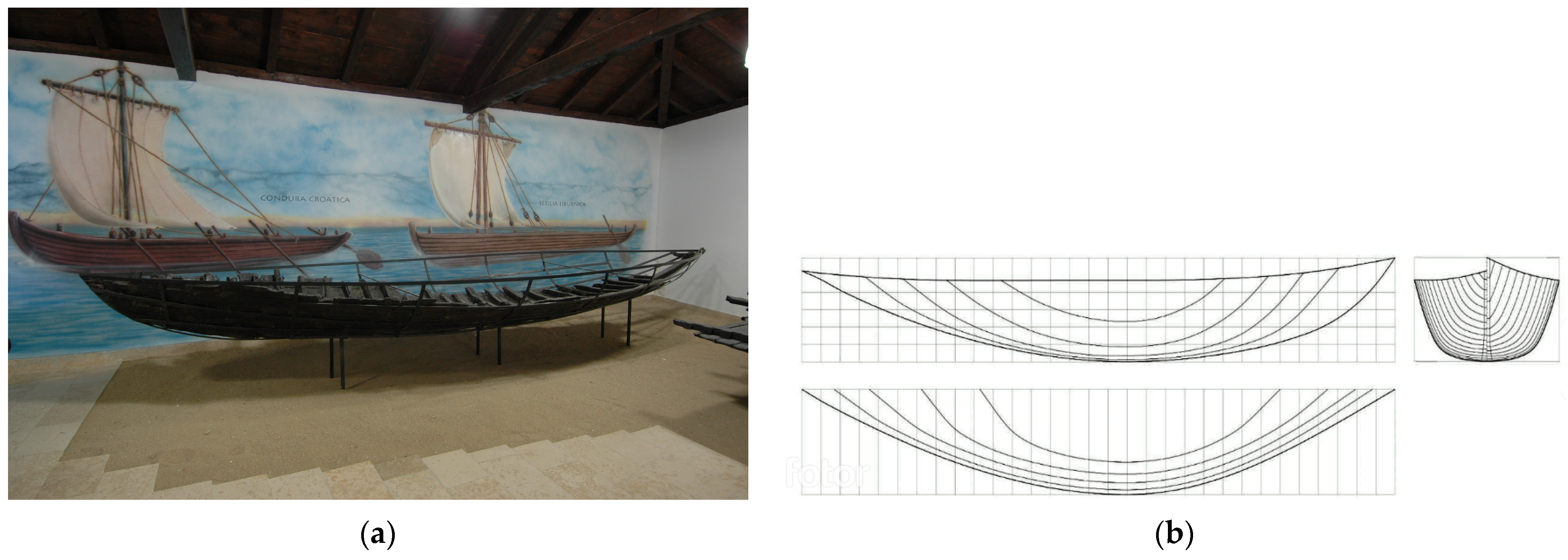
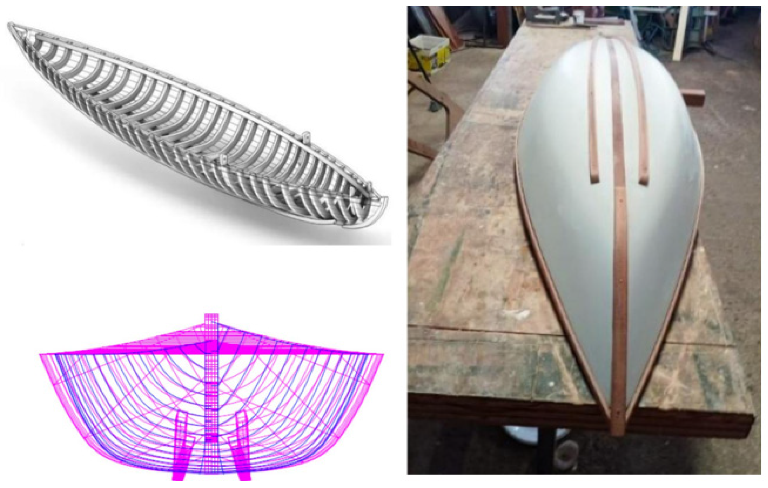
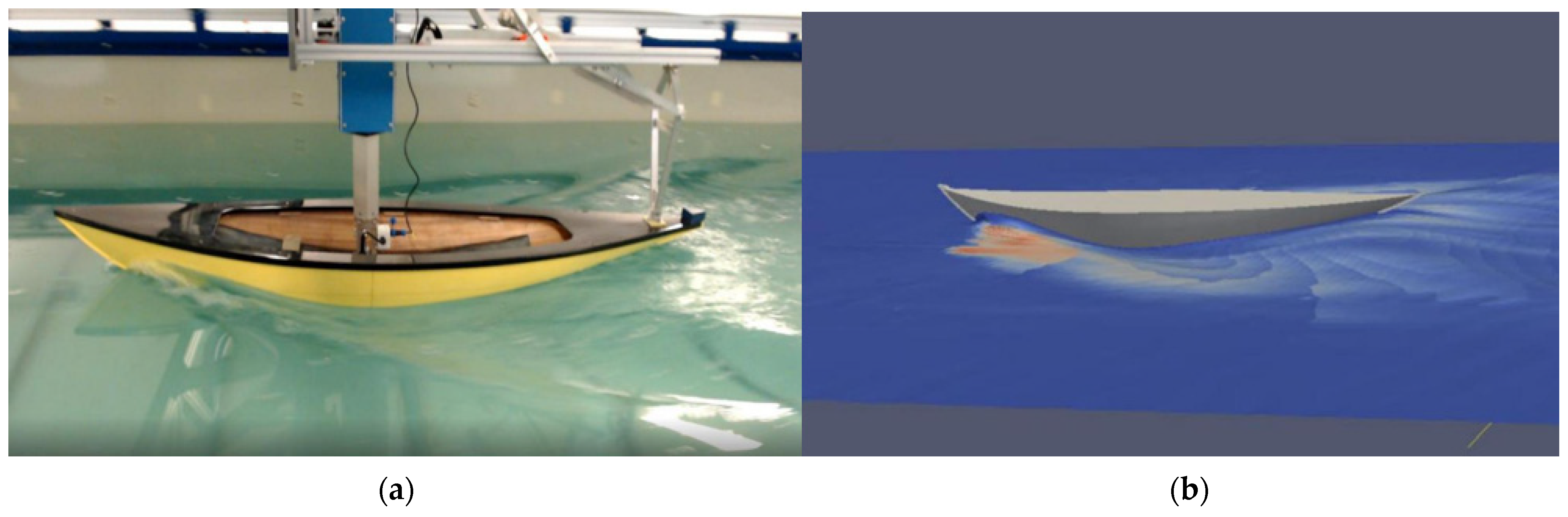
4.1. Case Study—Nin 1

In 1966, well-preserved remains of a medieval ship (Nin 1) were discovered near the port of the Croatian coastal town of Nin, north of Zadar. Two years later, the remains of another medieval ship (Nin 2) were spotted in the immediate vicinity. After several documentation campaigns, in 1974, the remains of the two ships were excavated and raised. After a long-term conservation process, which was carried out by the Zadar Archaeological Museum, they were exhibited in the Museum of Nin Antiquities. The first attempt at the reconstruction of the original hull lines was made by the conservator B. Vilhar in 1974, mainly for the needs of the museum display of preserved finds. The second reconstruction of the original hull lines was made by the naval architect I. Marinčić in the late 1990s, for the purpose of building two floating replicas. Marinčić’s work was based on the ships exhibited in the Museum and not on the original archaeological finds. For promotional purposes, the boats are today known as Condurae Croaticae [30].

The problem of hogging that affected the two replicas led to another reconstruction attempt, carried out by maritime historian M. Bondioli, within the NEREAS project (Numerical Reconstruction in the Archaeology of Seafaring, IP-2020-02-3420), funded by the Croatian Science Foundation [31], and the ship analysed in this study is based on these lines. The main characteristic of the structure of Nin ships is the lack of a keel and the existence of two almost parallel side elements that could serve as bilge keels. Besides that, they probably served as solid supports during low tide in the shallow sandy bay of Nin, and when pulling ships ashore. The Nin 1 museum exhibit as well as Bondioli’s proposal of the original hull lines are presented in Figure 1.

The main particulars of the life-size Nin 1 are stated in

Table 1. Ship particulars of the life-size Nin 1 (based on Bondioli’s proposal of the original hull lines).

Parameters	Lpp [m]	Height [m]	Mass [kg]	Tc [m]	Aw [m2]	$\nabla \mathit{c}$ [m3]
Value	7.8	0.6	1711	0.45	8.03	1.78
Parameters	Cp[-]	Lwl[m]	Bwl[m]	Cm[-]	LCBfpp[m]	LCFfpp[m]
Value	0.533	5.78	1.605	0.64	2.864	2.969

.

To conduct a series of experimental tests, the towing tank model of Nin 1 was created while respecting the geometrical constraints of the towing tank and the maximum loadbearing capacity of the towing tank equipment. This led to a model with a 1:4 ratio (λ = 4) to a life-size boat. The geometry model was made by the 3D CAD software Rhinoceros 7 [32]. After designing the CAD model, preliminary hydrostatic calculations were performed by AutoHydro 6. 5 [33], which takes into account hull shape, mass, and a centre of gravity, and it was determined that an additional 13 kg should be added to the ship’s original 7.9 kg. Hence, a design model draft equal to 11.25 cm (45 cm in life-size) could be reached. A ship model is made of mahogany and spray painted using a primer, which is a mixture of synthetic resin. Afterwards, two coatings are applied that serve as a protective layer. As the process of building a towing tank model requires a compromise between respecting idealized 3D CAD model geometry and a process of a physical model manufacture, a 10 mm hull thickness was chosen for building the towing tank model because of the simplicity of model realization and reaching the predetermined centre of gravity as well as a model weight, while thickness itself does not affect the accuracy of ship resistance calculation. A concise display of the towing tank creation consisting of CAD modelling and building is shown in Figure 2.

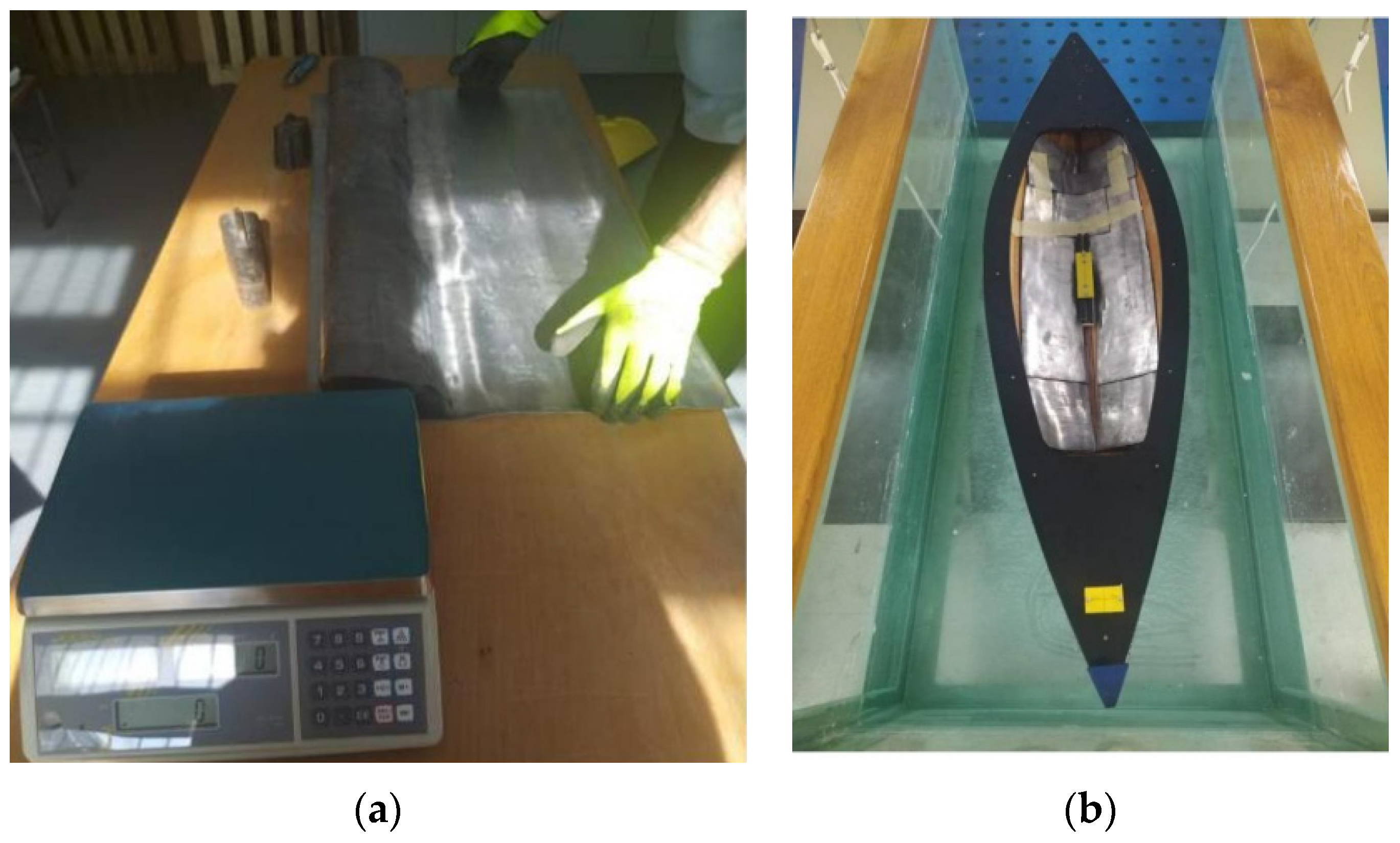
Towing Test Experiment

Towing test experiments were carried out at the University of Zagreb, Faculty of Mechanical Engineering and Naval Architecture. The overall dimensions of the towing tank are 32.8 m in length, 3.6 m in width and 1.8 m in depth. The towing tank is equipped with a carriage, beach, wave generator, wave probe and measuring equipment. No initial heel, drift or trim angle existed in the ship, and it was ballasted according to draft marks. Ship radius of inertia and longitudinal and vertical centres of gravity were measured and used as a base input for other calculations. The range of speed at which the model was tested was from 0.1 m/s up to 1.5 m/s, with 0.1 m/s increments. The initial hull surface roughness estimation was 150 μm. An experimental setup with model weighing, adding led strips, and determining accurate draft can be seen in Figure 3, while more detailed pieces of information on the towing tank model and tank water conditions are stated in

Table 2. Data of the experimental setup at t = 0 s.

Ship Parameters	Model Mass [kg]	Ballast [kg]	Towing Post Mass [kg]	Tc [m]	Aw [m2]	λ
Value	7.878	19.813	0.3	0.1125	0.502	4
Freshwater Parameters (by ITTC)	Temperature [°C]	Density [kg/m3]	Dynamic Viscosity [Pa·s]	Kinematic Viscosity [m2/s]	Vapour Pressure (MPa)
Value	20	998.2072	0.001002	1.0034 × 10−6	2.3393 × 10−3

.

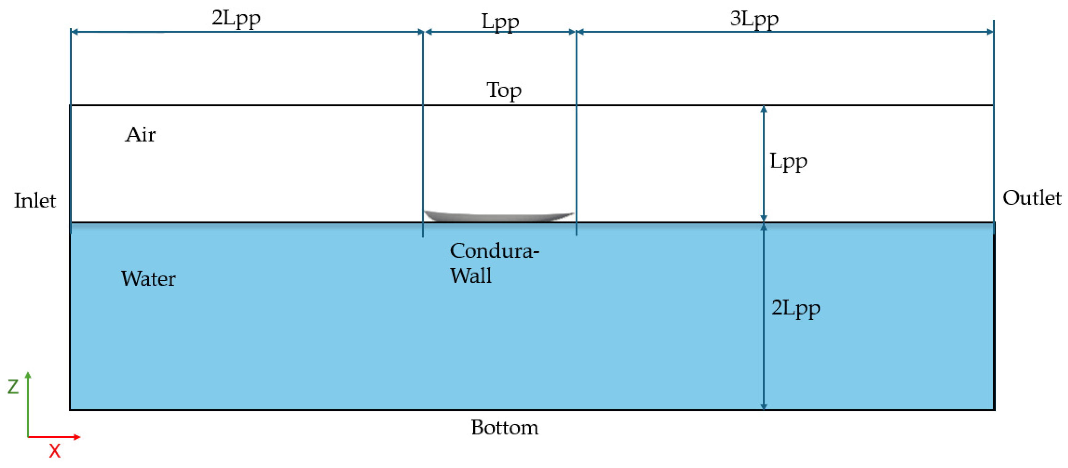
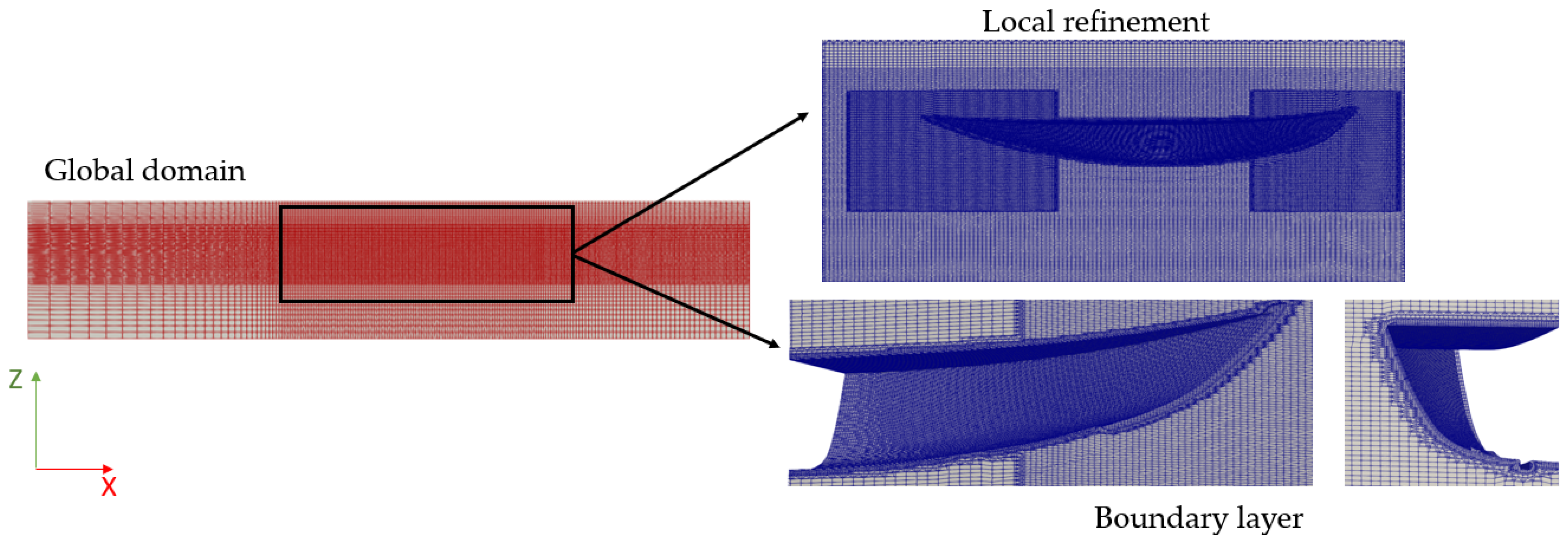
4.2. Numerical Approach—CFD

The numerical calculation of ship resistance requires the definition of the free surface, which allows the creation of waves during ship surges and consequently leads to correct resistance force calculation. In this study, open-source CFD software called OpenFOAM v9 [34] is used. As this software is primarily developed to solve complex fluid flow it is capable of successfully describing free surface and creation of waves during this condition. For this problem, an internally developed steady-state solver called LTSInterFoam is used. This solver is based on a Volume of Fluid method combined with the local time-stepping (LTS) algorithm, which maximizes the local time-step based on the local Courant number, thus making simulation quick and reliable. The side view of the numerical domain shown in Figure 4 consists of two phases, i.e., water and air, that are divided by a free surface. The domain in front of the ship is shorter than the domain behind the ship to leave more space for accurate wave creation. For the same reason, the width of the domain (y-direction) has an adequate length of 3Lpp.

Besides the applied boundary conditions stated in

Table 3. Boundary conditions for CFD analysis.

Boundary	Position	Boundary Condition
Inlet	3Lpp in front of the ship	Velocity inlet
Outlet	6Lpp in the back of the ship	Pressure outlet
Side	3Lpp side of ship	XZ symmetry
Top/bottom	3Lpp above/below the ship	XY symmetry
Nin 1	Lpp	Wall

, one set of numerical simulations was performed while accounting for surface roughness by using the already mentioned nutkRoughWallFunction function on the ship surface with roughness height Ks applied as 150 × 10⁻⁶ m and dimensionless roughness constant Cs applied as 0.5, which points out that roughness is uniform across the whole surface [35].

For both model-size as well as life-size ships, meshing attributes are identical. A global domain is meshed using a bias ratio of 0.3 in the X-, Y-, and Z-directions, which generates more cells in the area surrounding the ship, as shown in Figure 5 on the left. This approach improves the quality of the mesh. In the next phase of meshing, the ship’s geometry is introduced by “snapping” it into the domain, which is then precisely cut out. The final step in meshing involves adding boundary layers along this refined ship domain, as shown in Figure 5 on the right. The boundary layer mesh parameters were adjusted to ensure the y+ values have a minimum average of 50 for each velocity calculation. The y+ value is a non-dimensional number indicating the characteristics of the flow near the wall in turbulent conditions, and this adjustment is crucial for accurately capturing the effects of the turbulent boundary layer. As a result of these steps, the mesh includes an average of five boundary layer cells and totals 7.4 million cells

4.3. Empirical methods

4.3.1. Holtrop–Mennen

For calculating ship resistance by the Holtrop–Mennen method, Orca 3D 2.0.21 Software was used because of its already implemented Holtrop–Mennen procedure. As the approach with direct import of geometry offers less user definition, parameters defined either by software or the user are stated in

Table 4. Input data for Holtrop–Menne 1984 calculation.

Ship Parameters	k [-]	Lwl [m]	Bwl [m]	Displacement [kgf]	Aw [m2]	Am [m2]	Correlation Allowance [-]
Value	1.07	5.78	1.604	1834	8.035	0.58	0.002647
Ship Parameters	LCBF [%]	Λ [-]	Cp [-]	CB [-]	Lwl/Bwl [-]	Tc [m]	Bwl/Tc [-]
Value	0.477%Lwl	0.662	0.533	0.426	3.606	0.45	3.5309

. As previously mentioned, the Holtrop–Mennen method was developed for ships within a specific range of dimension ratios, namely, L_wl/B_wl and B_wl/T. When applying Holtrop–Mennen to ships outside these specified ranges, there is a potential risk of a decrease in accuracy, and it should be investigated. Software uses these parameters to assess wave coefficients and solve Equations (8)–(14).

4.3.2. Delft Systematic Hull Yacht Series (DSYHS)

While the viscous resistance is the same as in the case of Holtrop and ITTC [14], wave-making resistance is equal to polynomial expression by Equation (15), which uses coefficients a0–a7 to calculate force due to wave-making. The polynomial coefficients are obtained from previous research [36], which was based on a series of typical yacht hull designs that varied in length, width, and draft but only for a Froude number between 0.15 and 0.4. All polynomial coefficients are presented in

Table 5. Polynomial coefficients [36].

Fn	a0	a1	a2	a3	a4	a5	a6	a7
0.15	−0.0005	0.003	−0.0086	−0.0015	0.0061	0.001	0.0001	0.0052
0.2	−0.0003	0.0019	−0.0064	0.007	0.0014	0.0013	0.0005	−0.002
0.25	−0.0002	−0.0176	0.0031	−0.0021	−0.007	0.0148	0.0006	−0.0043
0.3	−0.0009	0.0016	0.0257	−0.0285	−0.036	0.0218	0.001	−0.0172
0.35	−0.0026	−0.0567	0.0446	−0.1091	−0.0807	0.0904	0.0014	−0.0098
0.4	−0.0074	−0.434	−0.15	0.0273	−0.1341	0.3578	0.0011	0.115

.

5. Results

The results will be presented graphically and using diagrams comparing model-size and life-size ships, whenever applicable. The results for the life-size ship are extrapolated using the aforementioned Equations (1)–(6) since measurements are obtained on the model-size ship. As not all four methods are applied to both models, the available results are summarized in

Table 6. Available results.

	Model-Size	Life-Size
Towing tank	YES	YES
CFD	YES	YES
Holtrop–Mennen	NO	YES
DHSYS	NO	YES

.

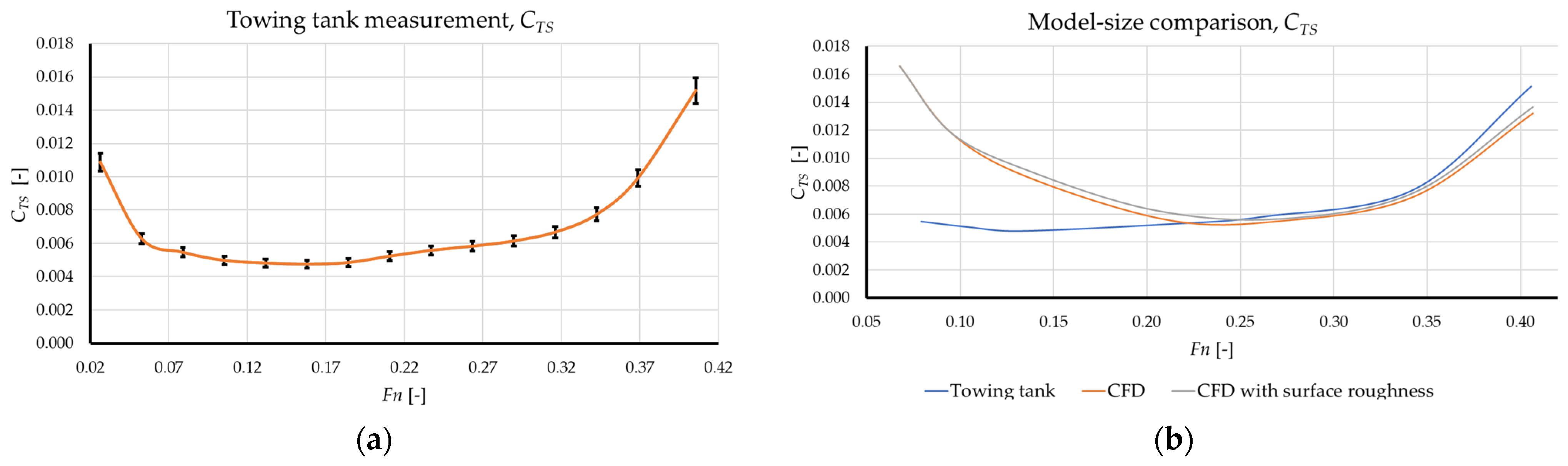
5.1. Model-Size Nin 1

First, a comparison between the towing tank and the CFD for the model-size Nin 1 is completed. This way, errors due to extrapolation are avoided and the CFD method is validated. In Figure 6, a visual comparison of wave generation at a maximum speed of 3 knots (6 knots for the life-size) is compared. It is visible that wave patterns occurring alongside the hull surface are identical between the experiment and CFD.

Next, a comparison of the total resistance coefficient between CFD and the towing tank experiment is shown in the diagram and table in Figure 7. The implementation of the surface roughness model leads to slightly better overlap with experimental results for the Froude number between 0.25 and 0.35. In the low-range velocity, results differ significantly between the towing tank and CFD.

A more detailed comparison of all three methods with standard deviation added to the towing tank results is presented in

Table 7. Detailed results of model-size comparison.

		Average Towing Tank Measurement		CFD			CFD—With Surface Roughness
v [knot]	Fn [-]	CTS [-]	RT [N]	CTS [-]	RT [N]	Standard Deviation [-]	CTS [-]	RT [N]	Standard Deviation [-]
0.5	0.06	0.0058	0.15	0.0166	0.3	0.00168132	0.0165	0.32	0.005606479
1	0.135	0.0048	0.4	0.008	0.65	0.00206743	0.00915	0.69	0.003114555
1.5	0.211	0.0052	0.96	0.005	1.02	0.00290492	0.00628	1.06	0.000812613
2	0.271	0.0059	1.68	0.0055	1.6	0.00346523	0.00563	1.7	0.000296827
2.5	0.342	0.0077	3.7	0.007	3.5	0.00495888	0.00752	3.6	0.00010675
3	0.4	0.0153	10	0.0132	8.9	0.001338702	0.01366	9.27	0.001146144

.

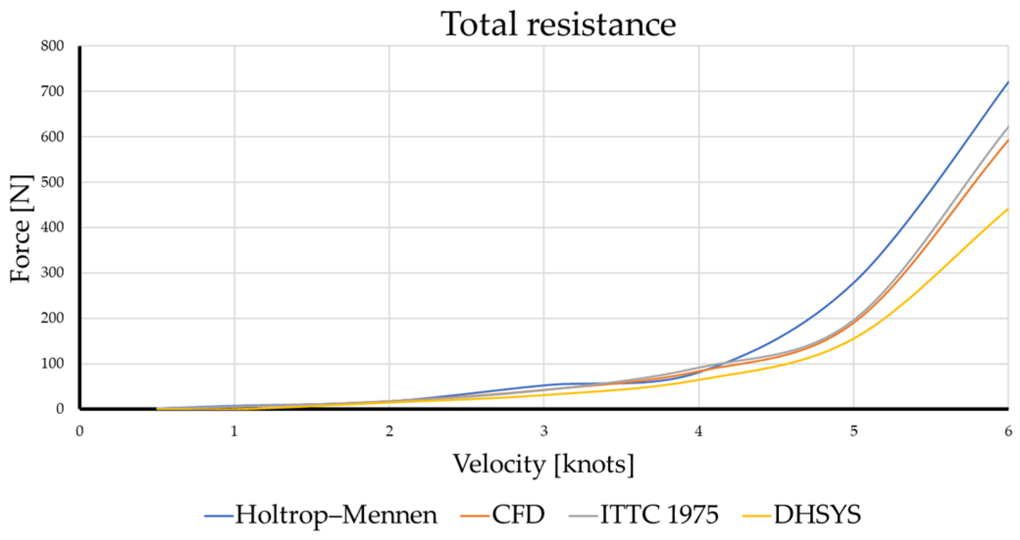
5.2. Life-Size Nin 1

The full resistance vs. velocity curve is presented next, as shown in Figure 8. To convert the velocity between the model and the full-size ship, the following equation is applied:

$$v_{life-size}={\mathrm{v}}_{\mathrm{m}\mathrm{o}\mathrm{d}\mathrm{e}\mathrm{l}-\mathrm{s}\mathrm{i}\mathrm{z}\mathrm{e}}·\sqrt{\lambda }$$

(16)

The difference between the extrapolated ITTC results and CFD calculation is less than 1% for the mid-velocity range (around 3 knots) and 5% for the high-velocity range (around 6 knots), while the biggest difference comes in the low-velocity area, up to 30%, even though absolute force values are extremely low in that range, being less than 0.5 N for the model-size.

The resulting difference between the experimental and the other three methods results can be seen in

Table 8. Comparative summary of all four methods.

ITTC 1975		CFD [%]		Holtrop–Mennen [%]		DHSYS
Velocity [knots]	Extrapolated Force from * TT [N]	RT [N]	Difference to ITTC [%]	RT [N]	Difference to ITTC [%]	RT [N]	Difference to ITTC [%]
0.5	1	2	100	2.1	64	-	-
1	5.1	5.5	7.8	7.8	52	-	-
2	16.8	18	7	17.8	5.7	15	−11
3	41.7	43	3.1	63.1	51	31.5	−24
4	91.4	84	−8	82	−10	65	−28
5	196	191	−2.9	280	42	156	−20
6	623	594	−4.6	722	15	442	−29

* TT = Towing tank.

. Experimental results are presented as a baseline for comparison.

Both empirical methods, Holtrop–Mennen and DHSYS, give significant result deviation compared with the baseline ITTC 1975 results extrapolated from the towing tank simulations for almost all velocity points. While both Holtrop–Mennen and DHSYS gave good overlap with towing tank results at 2 knots, they are inconsistent, and DHSYS underestimated every point. Thus, the focus will shift to a more detailed comparison between experimental and CFD results. In Figure 9 below, resistance is divided into the viscous and wave-making parts and compared between them. While viscous resistance quantitively follows the experimental results but with a slight offset, as shown in Figure 9, wave resistance differs in the mid-velocity region between 4 and 5 knots, as shown in Figure 9b.

Furthermore, a comparison of results with the applied surface roughness function (CFD) and extrapolation, Figure 10, showed a bigger discrepancy in the viscous force than when no surface roughness extrapolation was applied.

Table 9. Surface roughness comparison.

		ITTC 1978		CFD with Surface Roughness
Velocity [knots]	RT [N]	RV [N]	RW [N]	RT [N]/Difference to ITTC Results [%]	RV [N]/ Difference to ITTC Results [%]	RW [N] /Difference to ITTC Results [%]
0.5	2.1	1.42	0.3	3.55/47	2.55/80	1/42
1	6.1	4.6	1.5	7.5/22	4.95/6.6	2.55/69
2	22	17	5	23.2/5	16.7/−3	6.5/8
3	47	38	9	45/−5	34/−11	11/24
4	104	68	35	88/−15	59/−14	29/−17
5	218	107	110	205/−6	98/−8.6	107/−3.5
6	652	154	498	626/−4	141/−8	485/−2.6

presents a comparison between the CFD and towing tank results, focusing on the results with surface roughness. The results are broken down by component, and for each, the percentage difference between the calculated CFD component and its corresponding extrapolated component is provided. The discrepancies between CFD results and those from the extrapolation method ITTC 1978 based on surface roughness are larger than when surface roughness is not considered. This suggests that the CFD method tends to underestimate the viscous force component, leading to a greater deviation from the extrapolation method while prolonging simulation time due to convergence.

6. Discussion

As testing was also conducted in a low-velocity area at only 0.2 m/s, flow around the towing tank model is laminar due to its size difference, while in reality, turbulence occurs around the appendages. ITTC’s 1990 conference [37] prescribes that turbulence stimulators should be applied if appendages or bulbous bows exist in the model. Usually, these turbulence stimulators are made in the form of artificial objects such as Hama strips, sand grains, wires, or similar objects [38]. In this research, stimulators were applied in the form of strips of glue in the bow area, as shown in Figure 11a. The tests at low speeds between 0.2 knots and 2 knots (0.05–0.25Fn) were performed multiple times and showed significant percentual differences compared with the CFD results.

Even with added turbulence initialization, the biggest difference between the experimental towing tank tests and CFD calculations still occurred in the low-velocity region, as shown in Figure 11b. The probable cause of this is the measurement equipment and inherited tolerance in accelerometers due to measuring very small values, for both CFD and experiment resistance force, of less than 0.2 N, but the relative difference is significant at >30%.

7. Conclusions

This paper presents a comprehensive study of assessing the ancient ship Nin 1 resistance in calm water. The physical towing tank model of Nin 1 was produced on a 1:4 scale and tested in an experimental tank. Conducting each analysis led to the following conclusions:

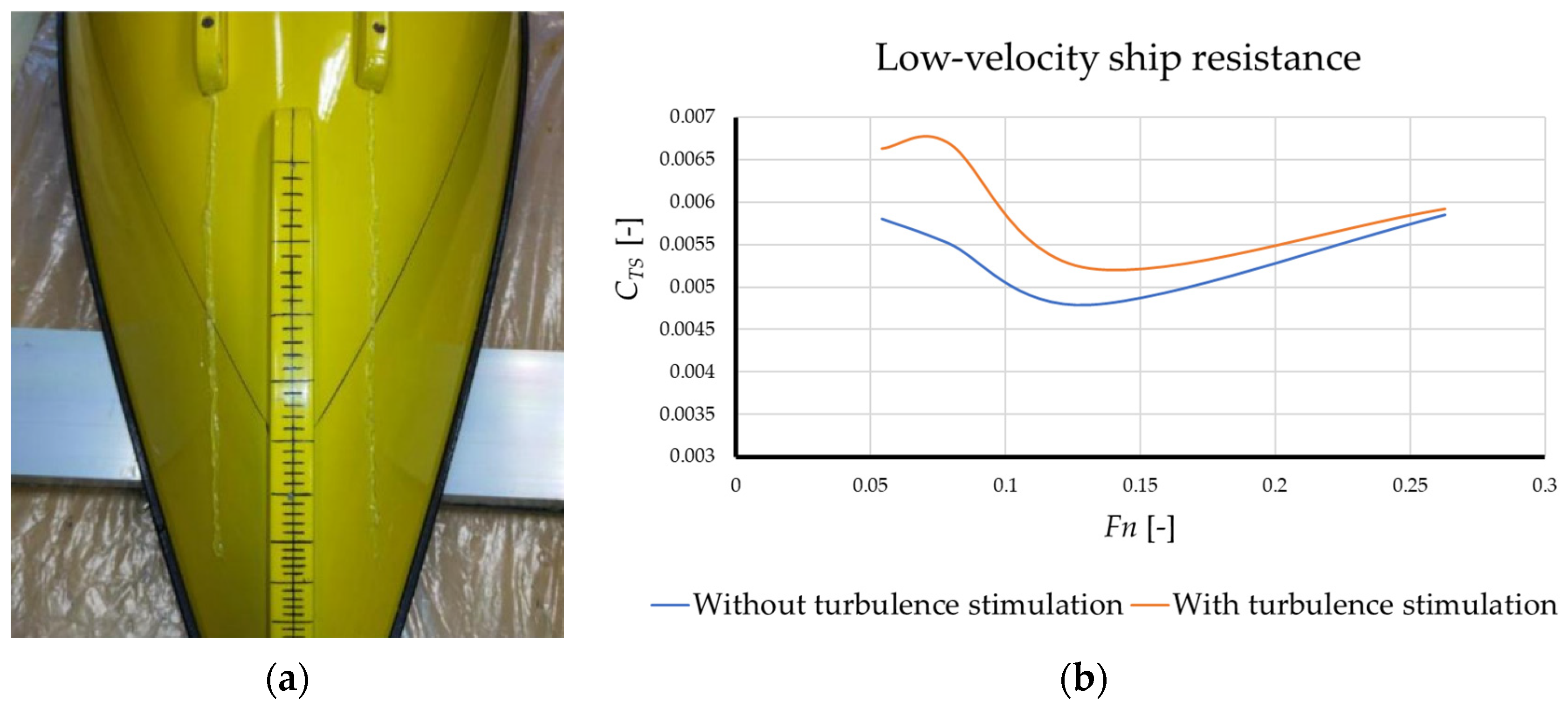
• CFD proved to be a reliable and accurate method for predicting ancient ship resistance. Differences between the experimental and CFD approach occurred in a very low-velocity range of >0.5 knots (0.25 m/s). As the CFD model converged after 1500 increments, the focus was shifted to testing equipment, which showed extreme sensitivity when dealing with a low-force reading of <0.2 N. This leads to the conclusion that standard accelerometers are not capable of reading extremely low values of force;
• An additional set of simulations performed with surface roughness showed that the implemented roughness model simply offsets the resistance curve and gives more accurate results in a model-size case;
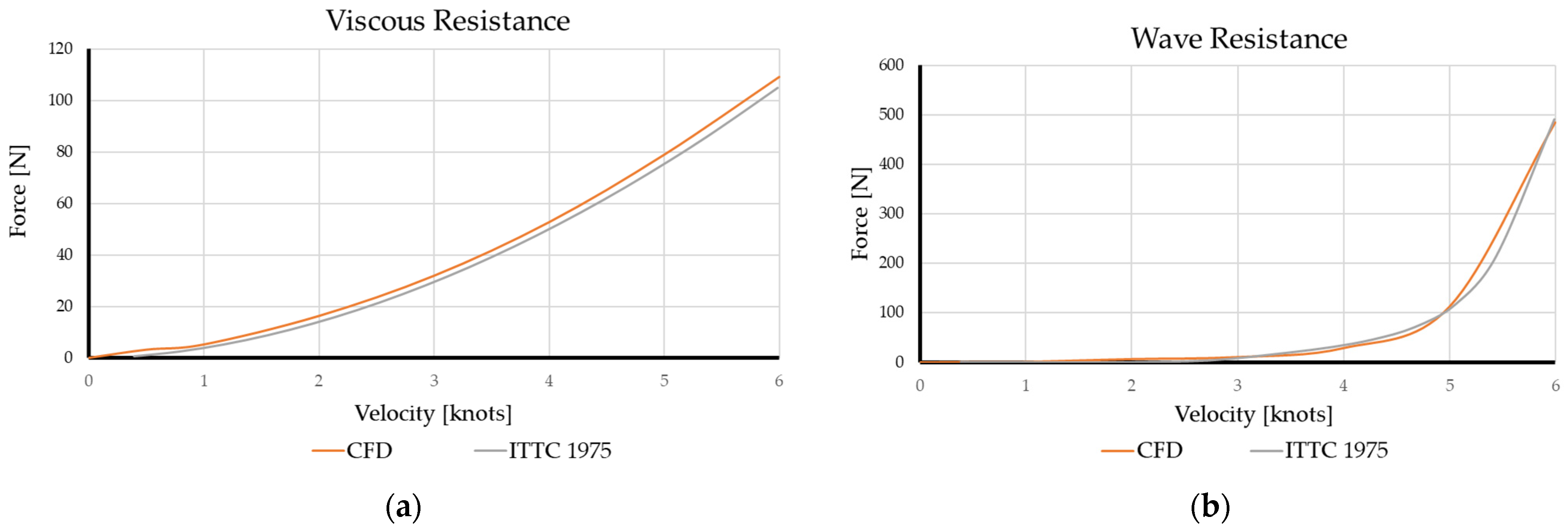
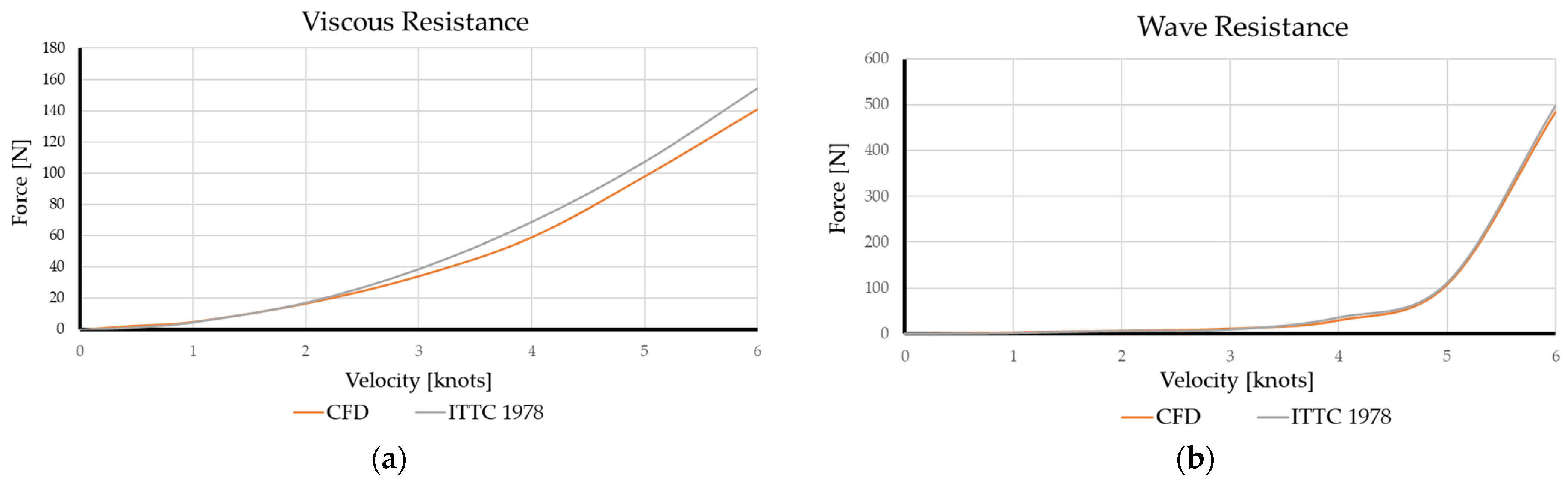
• When a comparison of resistance for the life-size Nin 1 was analysed, CFD again proved to be excellent in predicting resistance with significance only occurring in a low-velocity region;
• If surface roughness is applied in both extrapolation methods (ITTC 1978) as well in CFD, the difference between the results is higher;
• The Holtrop–Mennen method proved the suspicion that it is inefficient in predicting ship resistance for smaller boats with an average difference of 20% to experimental results and inconsistent agreement with the experimental results;
• Delft Yacht Hull Series showed better overlap than Holtrop–Mennen, with differences varying between 6 and 25%. The drawbacks of this method are insufficient data applicable to ancient ships as well as a velocity range that does not cover the whole Nin 1 assumed operational velocity range and thus, many other ancient ship velocities.

In conclusion, aside from direct experimental testing in a towing tank, the most dependable method for addressing these issues is employing the CFD (Computational Fluid Dynamics) approach without considering surface roughness. The CFD method proves reliable for both model-sized ships as well as when compared with extrapolated experimental outcomes on full-scale ships. The application of the empirical methods to ancient ships is inaccurate because those models were developed for ships with significantly different geometries.

References

1. Vosmer, T. The Jewel of Muscat Reconstructing a ninth-century sewn-plank boat. In Proceedings of the Forty-Fourth Meeting of the Seminar for Arabian Studies, London, UK, 22–24 July 2010; Volume 41, pp. 411–424. [Google Scholar]
2. Pomey, P.; Kahanov, Y.; Rieth, E. Transition from Shell to Skeleton in Ancient Mediterranean Ship-Construction: Analysis, problems, and future research. Int. J. Naut. Archaeol. 2012, 41, 235–314. [Google Scholar] [CrossRef]
3. Coates, J.F. Reconstructing the ancient Greek trireme warship. Endeavour 1987, 11, 94–99. [Google Scholar] [CrossRef]
4. Murray, W.M.; Ferreiro, L.D.; Vardalas, J.; Royal, J.G. Cutwaters Before Rams: An Experimental Investigation into the Origins and Development of the Waterline Ram: An Experiment in Ancient Cutwater Hydrographics. Int. J. Naut. Archaeol. 2017, 46, 72–82. [Google Scholar] [CrossRef]
5. Palmer, C. Windward Sailing Capabilities of Ancient Vessels. Int. J. Naut. Archaeol. 2009, 38, 314–330. [Google Scholar] [CrossRef]
6. Lasher, W.C.; Flaherty, L.S. CFD Analysis of the Survivability of a Square-Rigged Sailing Vessel. Eng. Appl. Comput. Fluid Mech. 2009, 3, 71–83. [Google Scholar] [CrossRef]
7. Ciortan, C.; Fonseca, N. Numerical Simulations of the Sails of a XVIth Century Portuguese Nau Marine 201. In Proceedings of the International Conference on Computational Methods in Marine Engineering, Lisbon, Portugal, 28–30 September 2011; pp. 278–289. [Google Scholar]
8. Rudan, S.; Radić Rossi, I. Numerička simulacija potonuća broda na temelju arheoloških zapisa. Archaeol. Adriat. 2020, 14, 129–157. [Google Scholar] [CrossRef]
9. Fawsitt, S.; Hobberstad, L.C. Computational Fluid Dynamics: Floating a Digital Barcode 02. Archaeonautica 2021, 21, 325–330. [Google Scholar] [CrossRef]
10. Subbaiah, B.V.; Thampi, S.G.; Rambabu, N.; Mustafa, V.; Akbar, M.A. Characterization and CFD Analysis of Traditional Vessels of Kerala. Int. J. Innov. Technol. Explore. Eng. 2020, 9, 132–149. [Google Scholar] [CrossRef]
11. Jerat, G.; Rudan, S.; Zamarin, A.; Rossi, I.R. Uncertainty in the Reconstruction of the Ancient Ship Hull and Its Impact on Sailing Characteristics. In Proceedings of the 16th International Symposium on Boat and Ship Archeology, Zadar, Croatia, 26 September–1 October 2021. [Google Scholar]
12. Handley, P. The Sutton Hoo Ship: Development and Analysis of a Computer Hull Model, Prior to Full-Scale Reconstruction. In Proceedings of the Historic Ships, London, UK, 7–8 December 2016; Royal Institute of Naval Architects: London, UK, 2016; pp. 137–147. [Google Scholar]
13. Tanner, P.; Whitewright, J.; Startin, J. The Digital Reconstruction of the Sutton Hoo ship. Int. J. Naut. Archaeol. 2020, 49, 5–28. [Google Scholar] [CrossRef]
14. International Towing Tank Conference (ITTC). Form Factor According to Prohaska. Proceedings of the 14th International Towing Tank Conference, ITTC’75, Ottawa, Canada, Volume 1. 1975. Available online: https://repository.tudelft.nl/islandora/object/uuid%3A9d57e745-61cc-4e9c-9f0d-c98c659059b2 (accessed on 1 April 2024).
15. International Towing Tank Conference (ITTC). ITTC—Recommended Procedures and Guidelines. 1978 ITTC Performance Prediction Method; 7.5-02-03; International Towing Tank Conference (ITTC): Zürich, Switzerland, 2017; Available online: https://www.ittc.info/media/8017/75-02-03-014.pdf (accessed on 1 April 2024).
16. Prohaska, C. A simple method for the evaluation of the form factor and the low speed wave resistance. In Hydro-and Aerodynamics Laboratory, Lyngby, Denmark, Hydrodynamics Section. In Proceedings of the 11th International Towing Tank Conference, ITTC’66, Tokyo, Japan, October 1966; Resistance Committee: Tokyo, Japan, 1966; pp. 65–66. [Google Scholar]
17. Bøckmann, E.; Steen, S. Model test and simulation of a ship with wavefoils. Appl. Ocean Res. 2016, 57, 8–18. [Google Scholar] [CrossRef]
18. Wang, J.; Yu, H.; Zhang, Y.; Xiong, X. CFD-based method of determining form factor k for different ship types and different drafts. J. Mar. Sci. Appl. 2016, 15, 236–241. [Google Scholar] [CrossRef]
19. van Chinh, H.; Thai, T.T. Improving the Accuracy of Ship Resistance Prediction Using Computational Fluid Dynamics Tool. Int. J. Adv. Sci. Eng. Inf. Technol. 2020, 10, 171. [Google Scholar] [CrossRef]
20. Pena, B.; Huang, L. A review on the turbulence modelling strategy for ship hydrodynamic simulations. Ocean. Eng. 2021, 241, 110082. [Google Scholar] [CrossRef]
21. Park, D.W.; Lee, S.B. The sensitivity of ship resistance to wall-adjacent grids and near-wall treatments. Int. J. Nav. Archit. Ocean. Eng. 2018, 10, 683–691. [Google Scholar] [CrossRef]
22. Van Nguyen, T.; Van Ngo, H.; Ibata, S.; Ikeda, Y. Effects of Turbulence Models on the CFD results of Ship Resistance and Wake. In Proceedings of the Japan Society of Naval Architects and Ocean Engineers, Hiroshima, Japan, 27–28 November 2017; Volume 25, pp. 199–204. [Google Scholar]
23. Matsuda, S.; Katsui, T. Hydrodynamic Forces and Wake Distribution of Various Ship Shapes Calculated Using a Reynolds Stress Model. J. Mar. Sci. Eng. 2022, 10, 777. [Google Scholar] [CrossRef]
24. Ge, G.; Zhang, W.; Xie, B.; Li, J. Turbulence model optimization of ship wake field based on data assimilation. Ocean. Eng. 2024, 295, 116929. [Google Scholar] [CrossRef]
25. Holtrop, J.; Mennen, G.G.J. An approximate power prediction method. Int. Shipbuild. Prog. 1982, 29, 166–170. [Google Scholar] [CrossRef]
26. Holtrop, J. A statistical re-analysis of resistance and propulsion data. Int. Shipbuild. Prog. 1984, 31, 272–276. [Google Scholar]
27. Holtrop, J. A statistical resistance prediction method with a speed dependent form factor. In Proceedings of the Scientific and Methodological Seminar on Ship Hydrodynamics (SMSSH ’88), Varna, Bulgaria, 1 October 1988. [Google Scholar]
28. Birk, L. Fundamentals of Ship Hydrodynamics: Fluid Mechanics, Ship Resistance and Propulsion; John Wiley Sons: Hoboken, NJ, USA, 2019; pp. 611–627. ISBN 978-1-118-85551-5. [Google Scholar]
29. Keuning, J.A.; Sonnenberg, U.B. Approximation of the Hydrodynamic Forces on a Sailing Yacht based on the Delft Systematic Yacht Hull Séries’. In Proceedings of the 15th International Symposium on “Yacht Design and Yacht Construction”, Amsterdam, The Netherlands, 16 November 1998; ISBN 90-370-01-71-8. [Google Scholar]
30. Radić Rossi, I.; Liphshitz, N. Analiza drvene građe srednjovjekovnih brodica iz Nina. Archaeol. Adriat. 2020, 10, 257–270. [Google Scholar] [CrossRef]
31. Nicolardi, M.; Bondioli, M.; Radić Rossi, I. The Contribution of Historical Sources in the Reconstruction of the Nin 1 Original Hull Form. In ISBSA 16, Sailing through History, Zadar 2021, Book of Abstracts.; Batur, K., Fabijanić, T., Radić Rossi, I., Eds.; University of Zadar: Zadar, Croatia, 2021; p. 105. [Google Scholar]
32. McNeel, R. Rhinoceros 3D, Version 6.0. Robert McNeel; Associates: Seattle, WA, USA, 2010. [Google Scholar]
33. AutoHydro Users Manual; Autoship Systems Corporation: Vancouver, BC, Canada, 2011.
34. Weller, H.G.; Tabor, G.; Jasak, H.; Fureby, C. A tensorial approach to computational continuum mechanics using object-oriented techniques. Comput. Phys. 1998, 12, 620–631. [Google Scholar] [CrossRef]
35. Speranza, N.; Kidd, B.; Schultz, M.P.; Viola, I.M. Modelling of hull roughness. Ocean. Eng. 2019, 174, 31–42. [Google Scholar] [CrossRef]
36. Keuning, L.J.A.; Katgert, M. A bare hull resistance prediction method derived from the results of The Delft Systematic Yacht Hull Series to higher speeds. In Proceedings of the International Conference Innovation in High Performance Sailing Yachts, Lorient, France, 29–30 May 2008. [Google Scholar]
37. ITTC. Report of the Resistance and Flow Committee. In Proceedings of the 19th International Towing Tank Conference, Madrid, Spain, 16–22 September 1990; Volume 1, pp. 62–64. [Google Scholar]
38. Lee, S.B.; Seok, W.; Rhee, S.H. Computational simulations of transitional flows around turbulence stimulators at low speeds. Int. J. Nav. Archit. Ocean. Eng. 2021, 13, 236–245. [Google Scholar] [CrossRef]
Figure 1. (a) Nin 1 in the Museum of Nin Antiquities. (b) CAD model (author: M. Bondioli).
Jmse 12 00658 g001
Figure 2. Nin 1—From CAD to physical model (authors: M. Bondioli/CAD, M. Jandrić/physical model).
Jmse 12 00658 g002
Figure 3. Nin 1: (a) led strips and model weighing and (b) conducting experimental tests.
Jmse 12 00658 g003
Figure 4. Setup of the numerical domain for CFD.
Jmse 12 00658 g004
Figure 5. Mesh domain.
Jmse 12 00658 g005
Figure 6. Wave generation at 3 knots: (a) towing tank and (b) CFD analysis.
Jmse 12 00658 g006
Figure 7. Results of the total resistance coefficient CTS: (a) towing tank and (b) model-size comparison.
Jmse 12 00658 g007
Figure 8. Total resistance forces with all four methods.
Jmse 12 00658 g008
Figure 9. Comparison between CFD and ITTC 1975 of (a) viscous resistance and (b) wave resistance.
Jmse 12 00658 g009
Figure 10. Surface roughness comparison between the CFD and experiment of (a) viscous resistance and (b) wave resistance.
Jmse 12 00658 g010
Figure 11. Turbulence simulation: (a) stimulators added with glue and (b) result comparison between 0.4 and 1 knot.
Jmse 12 00658 g011