Abstract
With the inception of the Argo program, the global ocean observation network is undergoing continuous advancement, with profiling buoys emerging as pivotal components of this network, thus garnering increased attention in research. In efforts to enhance the efficiency of profiling buoys and curtail energy consumption, a teardrop-shaped buoy design is proposed in this study. Moreover, an optimization methodology leveraging neural networks and genetic algorithms has been devised to attain an optimal profile curve. This curve seeks to minimize drag and drag coefficient while maximizing drainage, thereby improving hydrodynamic performance. Simulation-based validation and analysis are conducted to assess the efficacy of the optimized buoy design. Results indicate that the drag of the teardrop-shaped buoy with a deflector decreased by 9.2% compared to pre-optimized configurations and by 22% compared to buoys lacking deflectors. The hydrodynamic profile devised in this study effectively enhances buoy performance, laying a solid foundation for ocean thermal energy generation and buoyancy regulation control. Additionally, the optimized scheme serves as a valuable blueprint for the design of ocean exploration devices.
1. Introduction
In recent years, the scope of human exploration of the oceans has expanded significantly. The introduction of the Argo program, coupled with rapid advancements in underwater exploration technology, has created an enabling environment for the advancement of exploration buoys [1]. Currently, there are over 3000 profiling buoys actively operating in the ocean, making significant contributions to marine environmental observation, weather forecasting, and monitoring atmospheric changes, among other critical areas [2,3]. Conventional buoys rely on batteries for power, which cease functioning once their power is depleted. Consequently, leveraging ocean energy as a sustainable power source for buoys offers a promising solution to address their endurance limitations. Among the various ocean energy sources, ocean thermal energy stands out as one of the most abundant. It encompasses the thermal energy stored in the temperature differential between surface seawater and deep seawater, stemming from solar radiation. As a perpetual and readily accessible renewable energy source, ocean thermal energy holds significant potential for powering buoys and addressing their energy needs [4,5]. Therefore, the exploration of profiling buoys propelled by ocean thermal energy has emerged as a prominent research focus among scientists.
At present, a variety of profiling buoys have been developed. For instance, Sea-Bird Scientific has introduced NAVIS, which is a sleek cylindrical buoy outfitted with a suite of sensors including CTD sensor, optical sensor, and nitrate ultraviolet analyzer. Additionally, it features a built-in power supply enabling it to autonomously conduct 300 profile detections. However, this buoy has been susceptible to malfunctions due to flaws in the design of its hydraulic system [6]. The Scripps Institution of Oceanography has pioneered the development of the SOLO buoy series with various models enhancing efficiency and functionality. Notably, the SOLO-II model stands out as a lighter and more efficient iteration compared to its predecessors; it can carry out detection tasks in water depths of up to 2000 m. Furthermore, the SOLO-DEEP, an upgraded version of the SOLO-II, has achieved an impressive detection depth of 6000 m. Featuring an approximately spherical design, the SOLO-DEEP has successfully completed numerous missions in sea areas as deep as 4000 m off the coast of the United States of America [7,8]. Currently, APEX-type buoys, developed by the Webb company, stand as the most prevalent choice within the Argo program. Characterized by their spherical shape and platforms situated at each end for sensor mounting, these buoys have achieved remarkable milestones. They hold the record for ocean sounding depth, reaching an impressive 6000 m, and have consistently retrieved valuable data. [9]. In addition, operational buoys such as the NOVA buoy, a slender cylindrical design developed by MetOcean company [10], the NINJA buoy, featuring a cylinder with multiple segments rounded on one side and developed by the Agency for Marine-Earth Science and Technology and TSK company [11], and the ARVOR buoy, another slender cylindrical model developed by the Ocean Development Institute, have been successfully deployed [12]. The Ocean Profiling Explorer-COPEX, developed by the National Ocean Technology Center, has been employed in numerous ocean experiments, yielding satisfactory data results [13]. However, most buoy products are commercialized with limited public research, resulting in a scarcity of studies focused on optimizing buoy shapes. Most buoys in operation exhibit spherical or cylindrical shapes, which are prone to high resistance and consequently impact the carrying capacity of the buoy.
Similarly, the shape of underwater gliders driven by ocean thermal energy has also received attention in research. Nonetheless, there are references to various studies on the shape of underwater gliders, which also driven by ocean thermal energy that could serve as valuable resources. For instance, the Spray Glider developed by Sherman at the Scripps Institute of Oceanography features a slender, low-resistance streamlined shell [14] and boasts a maximum submerged depth of 1500 m [15]. The Slocum developed by WEBB measures 1.8 m in length and features a streamlined bow and tail. It is capable of operating at speeds of approximately 0.5 m/s in waters up to 200 m deep [16]. The Sea Glider developed by Erisken et al. at the University of Washington utilizes a spindle-like form factor with a smaller size, and it has also performed well in experiments [17]. Bertram and Alvarez conducted an in-depth discussion on the overall design simulation of the Autonomous Underwater Vehicle’s (AUV) shell. Collaborating with naval hydrodynamics experts, they put forth comprehensive guidelines for the shell shape, which are accompanied by empirical coefficients to optimize the maneuverability of the torpedo-like geometry [18]. Ye and Pan employed an enhanced ensemble of surrogates-based global optimization method (IESGO-HSR), which incorporates a hierarchical design space reduction strategy, to optimize the airfoils of the novel flying-wing configuration underwater glider [19]. Sun et al. used the efficient global optimization (EGO) method to achieve a higher maximum lift-to-drag ratio of the blender-wing-body underwater glider [20]. Fu et al. designed a slender ellipsoidal underwater glider and used a genetic algorithm to carry out multi-objective optimization of the hull drag and hull surface pressure for the underwater glider [21].
At present, most buoys in operation exhibit spherical or cylindrical shapes, which are prone to high resistance and consequently impact the carrying capacity of the buoy. Li introduced a streamlined buoy design that effectively enhanced float performance [22]. However, this design failed to account for the reciprocating motion characteristics of profiling buoys. Therefore, this paper proposes a water teardrop float inspired by the motion patterns of profiling buoys. This design incorporates a bow-like structure on both sides of the float to optimize its hydrodynamic performance. The key innovations of this study include: (a) The proposal and design of a teardrop profiling buoy, driven by ocean thermal energy, which considers buoy motion characteristics to enhance hydrodynamic efficiency during both ascent and descent phases. (b) Development of an optimization scheme for the buoy shell, with objectives focused on minimizing drag and drag coefficient while maximizing drainage volume. This approach aims to attain the optimal buoy shape for superior performance and improves buoy energy efficiency which will be crucial to maintaining and improving the Argo array [23]. These findings provide a solid foundation for the self-sustaining generation of ocean thermal energy and buoyancy regulation control for underwater buoys. Furthermore, they offer valuable insights for the development of underwater detection devices.
The remainder of this paper is organized as follows. Section 2 elucidates the theory employed in the design, computational fluid dynamics (CFD) simulation, and optimization process. Section 3 presents the optimization results following discussion, accompanied by an analysis of the hydrodynamic performance of the buoy. Finally, Section 4 offers concluding remarks.
2. Methods
To improve the hydrodynamic performance of the buoy, a teardrop buoy is proposed, designed, optimized and verified in this paper. This section primarily outlines the theoretical framework employed in the design of the buoy, CFD simulation, and optimization process. It is divided into three key parts: buoy structural design, numerical model development, and optimization scheme.
2.1. Buoy Structural Design
The shape of ocean exploration buoys typically resembles a rotational body. This rotational body is often described by a curve that rotates around an axis to form its surface, which is known as the generatrix. In this context, we introduce the teardrop curve as the generatrix of the rotational body. The teardrop curve is a streamlined curve resembling the edge of a water droplet, which is described as follows:
where represents the maximum radius, denotes the length of the front part, indicates the length of the ahead part, signifies the index of the front part, and represents the index of the ahead part.
The movement direction of a submarine in water aligns with its bow section, necessitating the design of the bow section curve to enhance control performance and reduce drag coefficient. Conversely, the stern section curve is typically designed to mitigate vortex formation at the stern. As ocean exploration buoys move vertically in seawater, both ends of the buoy alternate as the bow. Hence, this study proposes that both ends of the buoy feature teardrop-shaped curves with the design of the generatrix as follows:
where and determine the line shape of the teardrop curve. The curve is a straight line when and is nearly square when . To ensure that the research is accurate and effective and the scope of optimization is sufficient, the optimized range of values for and is constrained within the range of .
The ocean exploration buoy driven by thermal energy needs a certain amount of internal storage space. Therefore, the design process begins with confirming the internal space of the buoy shell before proceeding with the external structure design. Combined with the heat exchange system of the buoy, it is determined that the shell of the buoy will be a cylinder with a diameter of 246 mm and a height of 1400 mm. The heat exchange system requires 6 heat exchange tubes distributed around the shell. Comprehensive considerations of the buoy shape, water displacement, overall mass, and density of the deflector material lead to the adoption of a transitional structure for the buoy, which is segmented into front, middle, and back sections. The rotating busbar of the front and back sections of the deflector serves as the optimization object. The model of the buoy is depicted in Figure 1. The buoy is designed for a maximum diving depth of 1000 m, a maximum sailing speed of 1 knot (0.514 m/s), and a power generation rating of 300 W. The buoy’s internal capacity to carry equipment such as power generation systems, wireless communications, sensors, etc., as well as its external pressure-resistant capacity are considered; detailed dimensions are provided in Table 1.
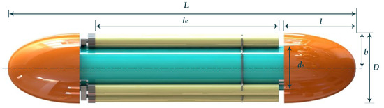
Figure 1.
The shape of the teardrop buoy.

Table 1.
Model parameters of the designed buoy.
2.2. Numerical Model
For the investigation of buoy hydrodynamic performance, accounting for fluid rotation and viscosity, the CFD method is employed. The CFD software Fluent is utilized for simulation purposes. This section outlines the governing equations of the CFD computational method, turbulence model selection, boundary conditions, and verification of mesh convergence.
2.2.1. Turbulence Model
As the buoy moves at a speed of , the Reynolds number reaches , surpassing a critical value. At this point, laminar flow will be disrupted and turbulence will be generated. In the turbulence model provided by ANSYS 2020 R2, the turbulent SST k−ω model exhibits better accuracy and stability in the near-wall region, allowing for a more accurate description of the flow field around the buoy. Therefore, the SST model has been chosen for this study. The SST is an optimized two-equation model that incorporates the equations for turbulent kinetic energy and turbulence frequency [24].
where is the rate of turbulence generation, , , , , , , is kinematic viscosity, d is the distance to the wall, and is turbulent viscosity, as follows:
2.2.2. Boundary Conditions
The boundary conditions and watershed dimensions for the CFD simulation are shown in Figure 2, while the dimensions of the buoy are shown in Table 1. This simulation is designed as a three-dimensional model with the computational domain measuring 6.94 m in length, 2.38 m in width, and 2.38 m in height. The left boundary is designated as the velocity inlet, while the right boundary is assigned as the pressure outlet. The buoy is positioned at the center of the computational domain with its surface defined as the wall. The fluid medium is seawater with a density of and a dynamic viscosity coefficient of at .
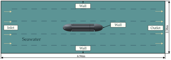
Figure 2.
CFD model condition.
2.2.3. Mesh-Independent Verification
To ensure accurate calculation of the flow field around the buoy, automatic inflation is employed in the automatic meshing process of ANSYS 2022 R2. Inflation is applied to the surface of the buoy with the number of layers set to 10. The first layer thickness is set to 2.5 with a growth rate of 1.2. Furthermore, the number and refinement of the mesh significantly impact the accuracy and computational speed of the calculations. Generally, finer meshes yield more accurate results, but an increase in mesh density also escalates computational workload, consequently reducing calculation speed. Hence, it is imperative to determine an appropriate mesh density. Four models with varying mesh sizes are investigated, which are each scaled by a factor of . The number of meshes and corresponding simulation results are summarized in Table 2:
Table 2.
Parameters of meshes and simulation result.
With all other parameters held constant, the computational results gradually converge as the number of meshes increases. When the number of grids reaches 321.1 w, both resistance and resistance coefficient have converged. Further increasing the number of meshes has minimal impact on result convergence. The difference in calculations between model 3 and model 4 is less than 1%. Considering computational efficiency, model 3 is selected as the mesh configuration for computation. The grid configuration is depicted in Figure 3.
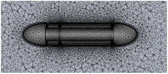
Figure 3.
Mesh of simulation with teardrop buoy.
2.2.4. Numerical Simulation Validation
To verify the CFD model presented in this paper, experiments conducted by Gao et al. [25] on an AUV in a circulating water tunnel are simulated. The model parameters are kept consistent with the aforementioned study except for the dimensions and shape of the submarine. The external dimensions of the AUV are depicted in Figure 4. Figure 5 illustrates that the CFD results closely align with the experimental findings with a maximum simulation error of 5.84%. This demonstrates the accuracy of the numerical simulation. Consequently, the simulation results and optimization scheme based on this numerical model can be considered reliable.
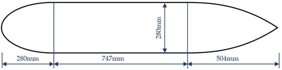
Figure 4.
The dimension and shape of the AUV by Gao et al. [25].
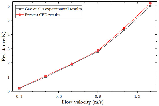
Figure 5.
Comparison of resistance between CFD simulation and Gao et al.’s experiment result [25].
2.3. Optimization Scheme
When optimizing the shape of the buoy, the primary objective is to reduce water resistance while the buoy moves through seawater. Additionally, the deflector is crafted using lightweight materials to provide extra buoyancy while minimizing buoy resistance. However, an excessively large deflector may impede buoy operations and increase the complexity of buoy deployment. Therefore, the optimization objective is to achieve lower resistance and increased drainage volume under these constraints. Figure 6 illustrates the optimization process: initial parameters obtained through Latin hypercube sampling are simulated to create an initial sample, which is followed by training the samples with a neural network to establish a fitted functional relationship. Subsequently, a genetic algorithm is employed to identify Pareto optimal solutions and plot the Pareto front. Finally, the optimal buoy shape is determined following CFD verification.
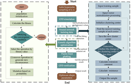
Figure 6.
Optimization solution flowchart.
2.3.1. Building Performance Analysis Functions with Neural Networks
Based on the optimization objectives outlined above, this paper will employ a radial basis neural network to examine the relationship between the values of and and the water resistance, resistance coefficient, and drainage volume of the buoy during its movement. This analysis aims to explore the connection between the generatrix of the buoy and its hydrodynamic performance.
Neural networks are mainly composed of input, hidden and output layers. The neural network training process is shown on the right side of Figure 4. The training principle is shown in Algorithm 1; Sample A is used as a training set, from which vectors are selected and used as the center of the radial function base. The mean square error is minimized through gradient descent, and iterations continue until the error value meets satisfaction. Subsequently, the functional relationship between , and resistance are outputted.
| Algorithm 1: Neural network fitting the functional relationship between,and resistance. |
| INPUT: Training set D = {(, )} i = 1, 2, …30 |
| Learning rate η = 0.001 |
| Radial basis network based on (, ) REPEAT |
| FOR ALL (, ) IN D Calculate the error from the network parameters to the output layer; |
| Calculate the descending gradient of the network parameters based on the error; |
| Update the parameters according to the descending gradient; |
| END FOR |
| UNTIL mean square error < 0.01 |
| OUTPUT the functional relationship between , and resistance |
The input layer is:
The Gaussian function is chosen as the radial basis function for the hidden layer due to its fast approximation and simple structure. The hidden layer function can be expressed as
where i is the implied layer node number, denotes the radial basis function center vector at the ith node, and is the radial basis function node width. Combining the above equations and introducing the weight vector w, the output layer y is
2.3.2. Genetic Algorithm
Genetic algorithms are search algorithms that mimic natural evolution and heredity. They search for and improve the optimal solution by performing operations such as selection, crossover, and mutation on individuals within the population. The optimization search principle is outlined in Algorithm 2: after initializing , the fitness is calculated, individuals are selected based on their fitness, and then they are subjected to crossover and mutation. The resulting individuals are added to the new generation of the population, and the process repeats until the number of evolutionary generations reaches 500. The minimum and its corresponding , values are then outputted. The size of the initial population significantly affects the efficiency of the optimization search. A population that is too small can make it difficult to find the best solution for the optimization problem, whereas a large population may be inefficient and time consuming due to processing numerous unnecessary individuals. Therefore, in this study, the population size is set to 100, the optimal individual coefficient of the genetic algorithm is 0.4, the maximum number of evolutionary generations is 500, and the deviation of the fitness function is set to .
| Algorithm 2: Genetic algorithm for finding the minimum resistance value. |
| BEGIN |
| Initialize (0) t = 0; Initialize parameters |
| While (t < 500) do |
| Calculate individual fitness; |
| Select individuals from the population based on fitness; |
| Perform crossover and mutation of selected individuals; |
| Add manipulated individuals to the population; |
| UNTIL t = 500 evolutionary generations up to 500 |
| END |
| OUTPUT minimum |
2.3.3. Pareto Optimal Solution
Under the given constraints, the task of optimizing multiple objectives to attain their maximum (or minimum) values is referred to as a multi-objective optimization problem. The essence of solving such a problem lies in identifying a set of non-inferior solutions, known as Pareto-optimal solutions, which strive to achieve a balanced outcome across individual objectives. The collection of multiple Pareto-optimal solutions plotted in the objective function space forms what is known as the Pareto front.
Assuming that the multi-objective optimization problem involves N variables, T optimization objectives, R inequality constraints, and K equality constraints, the expression is as follows:
where , X is the space of design variables; , Y is the target space; is the inequality constraint; and is the equality constraint.
In this paper, the motion data of buoys with varying slewing body buses are utilized as inputs, and a radial basis neural network is trained to establish the relationship between the control parameters of the slewing body buses and the motion performance of the buoys. This relationship serves as the objective function output. Consequently, the shape optimization problem of the buoys is transformed into a multi-objective optimization problem involving the performance parameters of the buoys. The set of Pareto optimal solutions will be determined based on minimizing drag, minimizing drag coefficient, and maximizing drainage volume as the objectives.
3. Results and Discussion
In this section, the simulation results of the buoy’s hydrodynamic performance are presented. The parameter optimization process is described in detail, aiming to minimize drag, minimize drag coefficient, and consider drainage volume. The optimized parameters are then simulated in Fluent to verify the hydrodynamic performance of the optimized buoys.
3.1. Sampling and CFD Simulation Results
Firstly, the initial shape of the buoy is simulated and analyzed. The seawater flow velocity is set as , , , and . The resulting drag force and drag coefficient of the buoy during its profile movement in seawater are shown in the Table 3 below.
Table 3.
Kinematic energy parameters of bouy at different speeds.
When the velocity of the buoy was increased from 0.1 to 0.3 m/s, the drag on the buoy increased by 2.19 N, and from 0.3 to 0.5 m/s, the drag increased by 4.6 N. According to the formula:
The skin bag needs to provide a volume change of about 245 mL for the buoy to undergo profiling motion at a velocity of 0.3 , where is the buoyancy on the buoy, and is the buoy drainage volume. When the buoy is moving at a velocity of 0.5 m/s, the skin bag needs to provide a volume change of about 705 mL. However, the size of the skin bag is too large, occupying space inside the shell and requiring additional heat exchangers for operation. Therefore, optimizing the shape of the buoy to minimize drag, skin friction, and energy consumption is essential for enhancing buoy performance.
Secondly, the Latin hypercube sampling method combines random sampling with stratified sampling, providing a strong representation of samples across the overall probability distribution. This method yields statistically accurate results with small sample sizes [26], thereby achieving better sampling accuracy while utilizing smaller computational costs. Moreover, it ensures accurate representation of remote events in the sampling process. Therefore, the Latin hypercube sampling method is employed to generate 30 sets of curves, which are then used to simulate the hydrodynamic performance of the buoy in Fluent at 0.5 m/s. The curve parameters and simulation results are denoted as sample A. The spatial distribution of the 30 sets of samples taken is shown in Figure 7, and several examples are represented in Table 4.
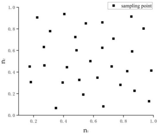
Figure 7.
Spatial distribution of the sample.
Table 4.
Performance parameters of several samples in sample A.
The maximum value in minimum distance and minimum potential energy are used to discuss the accuracy of the randomization of the Latin hypercube sampling method, as shown below:
where is the distance between sample i and sample j.
It is calculated that is 0.105, and is 4041.3. Upon assessing the indicators and the sample distribution shown in Figure 7, it is evident that the Latin hypercube sampling method ensures the randomness of the sample. Given the complex and non-linear functional relationship between resistance and curve parameters, it is essential to utilize the simulation results from the 30 sets of sample parameters as training data for the neural network to accurately capture this relationship.
3.2. Neural Network Training Results
The relationship between the parameter , and the drag force on the buoy profile during motion is fitted to the data using the radial basis neural network described in Section 2.3.1. Thirty sets of buoy parameters with different slewing buses from the table are used as training data and inputted into the neural network for iterative computation. The relationship between the parameters , and the resistance of the buoy is finally obtained, as shown in Figure 8. It can be seen that there exists a certain set of defined and unique values within a specific range that minimizes the resistance to movement of the buoy. However, numerous saddle points exist in the surface function, making the gradient descent method unsuitable for searching the optimal value as it may lead to falling into local optima.
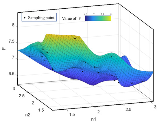
Figure 8.
Neural network training result.
3.3. Optimal Solution Selection
Based on the global search results obtained from the genetic algorithm, the Pareto front is plotted, as shown in Figure 9. The Pareto solution set is determined based on criteria such as the minimum resistance, the minimum resistance coefficient, and the maximum drainage volume. Finally, five sets of parameters are selected, as illustrated in Table 5.
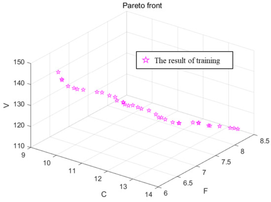
Figure 9.
Pareto frontier of the optimization in this study.
Table 5.
Optimal solution set of curve parameters.
In the optimal solution set, the first group exhibits the smallest drag of 6.36 N with a corresponding resistance coefficient of 10.308. Additionally, its drainage volume measures 137.994 L. On the other hand, the second group records a resistance of 6.401 N and a resistance coefficient of 10.457, albeit with a higher drainage volume of 141.169 L, representing a 3.75 L increase compared to the first group. According to Equation (15), the load of the second group is increased by 3.75 kg compared to the first group. Remarkably, despite this increase in load, the resistance is only raised by 0.041 N. Consequently, the skin bag needs to provide a volume change of about 4 mL for the buoy to execute profiling motion. In summary, while the second group exhibits similar resistance to the first group, with both being significantly lower than the initial value, the second group boasts the highest load capacity. Hence, the parameters of the second group are deemed optimal.
3.4. Simulation Verification
According to the optimization results, the rotary generatrix is obtained as follows:
Fluent simulation is utilized to validate the plausibility of the results obtained from neural network fitting. At a flow velocity of 0.5 m/s, corresponding to the profiling velocity of the buoy, the simulated resistance on the buoy is 6.41 N. Comparatively, the fitted value obtained from the neural network is 6.401 N, resulting in a fitting error of approximately 0.14%. Additionally, Figure 10 illustrates the velocity streamline around the buoy, showcasing uniform flow velocity and stable flow lines. Consequently, the fitting function of the neural network and the optimization scheme are deemed credible. In comparison to the initial sample drag of 7.05 N, the optimized buoy drag experiences a reduction of 9.2%. Moreover, when compared to buoys lacking a deflector, the optimized buoy demonstrates a 22% reduction in resistance. This optimized solution effectively minimizes the resistance of the buoy while ensuring maximum drainage volume and stable flow field around the buoy with uniform flow velocity. Furthermore, in contrast to Li’s streamlined buoy [24], the proposed and optimized teardrop buoy better aligns with the reciprocating motion characteristics of the buoy, thereby enhancing its performance during both descent and ascent. This optimized design is more practical and efficient.
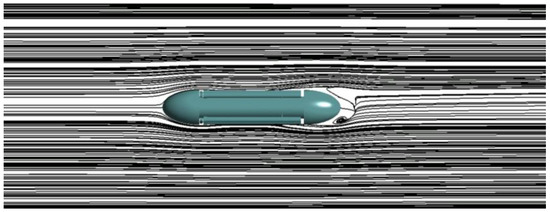
Figure 10.
Velocity streamlines at the flow rate of 0.5 .
To visually demonstrate the hydrodynamic performance of the buoy, velocity fields around the buoy are compared at different flow velocities ranging from 0.1 to 0.6 m/s, as depicted in Figure 11. The optimized teardrop buoy maintains a stable flow field even at low velocities, as observed in Figure 11a–d. Moreover, the flow field remains stable as the velocity increases, which is illustrated in Figure 11e,f. Noticeably, a small region of low velocity is observed at the top of the bow with slightly elevated flow velocities at the ends of the deflector. Fluid along the structural path of the device is compelled to form vortices around the edges, resulting in energy dissipation, which is known as form drag. The teardrop-shaped deflector serves to reduce boundary layer separation, mitigate backflow and vortex action, and consequently decrease pressure differential resistance. Additionally, the smooth passage of surface fluid minimizes the creation of vacuum zones on the buoy’s surface, effectively reducing pressure differences that may be generated in this area. This reduction in resistance contributes to the superior hydrodynamic performance of teardrop-shaped buoys.
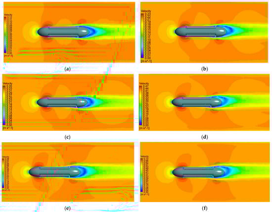
Figure 11.
Velocity field around the teardrop buoy: (a) 0.1 ; (b) 0.2 ; (c) 0.3 ; (d) 0.4 ; (e) 0.5 ; (f) 0.6 .
4. Conclusions
This paper investigates the motion characteristics of buoys propelled by ocean thermal energy. Given the significant impact of the deflector shape on buoy performance, which directly influences operational efficiency and payload capacity, a teardrop buoy design is proposed and developed. Subsequently, a multi-objective optimization scheme, integrating genetic algorithms and neural networks, is formulated to minimize drag.
Firstly, a numerical simulation platform was established in Fluent, mirroring wind tunnel tests. Detailed descriptions of boundary conditions and mesh division procedures were provided. Thirty sample sets for , are generated using the hypercubic sampling method and then simulated in Fluent to analyze buoy resistance and drag coefficients under varied parameters.
Furthermore, data are trained using a radial basis neural network to establish a functional relationship between parameters and drag. Results indicated the presence of a unique , value that minimizes buoy resistance. Multi-objective optimization of the shell of the buoy, focusing on hydrodynamic performance and drainage volume, is conducted through a combination of genetic algorithms and Pareto front analysis, yielding optimal values for and as well as the buoy shell curve.
Finally, optimization results are verified in Fluent. Simulation outcomes demonstrate that the optimized shell reduces buoy resistance by 9.2% during seawater profile movement at 0.5 m/s, and by 22% compared to buoys lacking a deflector. This enhancement in motion performance and reduction in energy consumption in similar operational states provide a strong foundation for self-sustaining ocean thermal energy generation and buoyancy regulation control in underwater buoy applications.
Author Contributions
Conceptualization, D.Z. and W.S.; methodology, D.Z.; software, D.Z.; validation, D.Z. and Z.Z.; formal analysis, D.Z.; investigation, Z.Z.; resources, S.L.; data curation, D.Z. and W.S.; writing—original draft preparation, D.Z.; writing—review and editing, D.Z., W.S., F.G. and S.L.; visualization, Z.Z.; supervision, W.S.; project administration, S.L.; funding acquisition, S.L. All authors have read and agreed to the published version of the manuscript.
Funding
This research was funded by the National Key Research and Development Program of China under Grant 2023YFC2810000, the National Natural Science Foundation of China under Grant 52175054 and the Shandong Province Science and Technology-oriented Small and Medium-sized Enterprises (SMEs) Innovation Capacity Enhancement Project under Grant 2023TSGC0320 and 2022TSGC2172.
Institutional Review Board Statement
Not applicable.
Informed Consent Statement
Not applicable.
Data Availability Statement
Dataset available on request from the authors.
Conflicts of Interest
The authors declare no conflict of interest.
References
- Xing, X.G.; Claustre, H. Toward deeper development of Biogeochemical-Argo floats. Atmos. Ocean. Sci. Lett. 2018, 11, 287–290. [Google Scholar] [CrossRef]
- Potiris, M.; Mamoutos, I.G.; Tragou, E.; Zervakis, V.; Kassis, D.; Ballas, D. Dense Water Formation in the North—Central Aegean Sea during Winter 2021–2022. J. Mar. Sci. Eng. 2024, 12, 221. [Google Scholar] [CrossRef]
- Hu, Y.; Shao, W.; Li, J.; Zhang, C.; Cheng, L.; Ji, Q. Short-Term Variations in Water Temperature of the Antarctic Surface Layer. J. Mar. Sci. Eng. 2022, 10, 287. [Google Scholar] [CrossRef]
- Abbas, S.M.; Alhassany, H.D.S. Review of enhancement for ocean thermal energy conversion system. J. Ocean. Eng. Sci. 2023, 8, 533–545. [Google Scholar] [CrossRef]
- Herrera, J.; Sierra, S. Ocean Thermal Energy Conversion and Other Uses of Deep Sea Water: A Review. J. Mar. Sci. Eng. 2021, 9, 356. [Google Scholar] [CrossRef]
- Barnard, A.H.; Mitchell, T.O. Biogeochemical monitoring of the oceans using autonomous profiling floats. Ocean News Technol. 2013, 19, 16–17. [Google Scholar]
- Roemmich, D.; Johnson, G.C.; Riser, S. The Argo Program: Observing the global ocean with profiling floats. Oceanography 2009, 22, 34–43. [Google Scholar] [CrossRef]
- Roemmich, D.; Sherman, J.T.; Davis, R.E. Deep SOLO: A full-depth profiling float for the Argo Program. J. Atmos. Ocean. Technol. 2019, 36, 1967–1981. [Google Scholar] [CrossRef]
- Petzrick, E.; Truman, J.; Fargher, H. Profiling from 6000 meter with the APEX-Deep float. In Proceedings of the Oceans 2013 MTS/IEEE San Diego, San Diego, CA, USA, 23–27 September 2013. [Google Scholar]
- Kobayashi, T.; Amaike, K.; Watanabe, K. Deep NINJA: A new float for deep ocean observation developed in Japan. In Proceedings of the 2011 IEEE Symposium on Underwater Technology and Workshop on Scientific Use of Submarine Cables and Related Technologies, Tokyo, Japan, 5–8 April 2011. [Google Scholar]
- Gould, W.J. From swallow floats to Argo—The development of neutrally buoyant floats. Deep Sea Res. Part II Top. Stud. Oceanogr. 2005, 52, 529–543. [Google Scholar] [CrossRef]
- André, X.; Moreau, B.; Reste, S.L. Argos-3 Satellite Communication System: Implementation on the Arvor Oceanographic Profiling Floats. J. Atmos. Ocean. Technol. 2015, 32, 1902–1914. [Google Scholar] [CrossRef]
- Yu, L.Z.; Zhang, S.Y.; Shang, H.M. Progress of China Argo float. Ocean. Technol. 2005, 2, 121–129. [Google Scholar]
- Sherman, J.; Davis, R.E.; Owens, W.B.; Valdes, J. The autonomous underwater glider “spray”. IEEE J. Ocean. Eng. 2001, 126, 437–446. [Google Scholar] [CrossRef]
- Davis, R.E.; Eriksen, C.C.; Jones, C.P. Autonomous buoyancy-driven underwater gliders. In The Technology and Applications of Autonomous Underwater Vehicles; Griffiths, G., Ed.; Taylor and Francis: London, UK, 2002; pp. 37–58. [Google Scholar]
- Webb, D.C.; Simonetti, P.J.; Jones, C.P. SLOCUM: An underwater glider propelled by environmental energy. IEEE J. Ocean. Eng. 2001, 26, 447–452. [Google Scholar] [CrossRef]
- Eriksen, C.C.; Osse, T.J.; Light, R.D. Seaglider: A long-range autonomous underwater vehicle for oceanographic research. IEEE J. Ocean. Eng. 2001, 126, 424–436. [Google Scholar] [CrossRef]
- Bertram, V.; Alvarez, A. Hydrodynamic Aspects of AUV Design 2006. Available online: https://www.researchgate.net/publication/228395786 (accessed on 5 April 2024).
- Ye, P.; Pan, G. Shape optimization of a blended-wing-body underwater glider using surrogate-based global optimization method IESGO-HSR. Sci. Prog. 2020, 103, 0036850420950144. [Google Scholar] [CrossRef] [PubMed]
- Sun, C.; Song, B.; Wang, P. Parametric geometric model and shape optimization of an underwater glider with blended-wing-body. Int. J. Nav. Arch. Ocean Eng. 2015, 7, 995–1006. [Google Scholar] [CrossRef]
- Fu, X.; Lei, L.; Yang, G.; Li, B. Multi-objective shape optimization of autonomous underwater glider based on fast elitist non-dominated sorting genetic algorithm. Ocean Eng. 2018, 157, 339–349. [Google Scholar] [CrossRef]
- Li, Z.; Liu, Y.; Guo, F.; Xue, G.; Li, S.; Li, X. Multi-objective optimization of the shell in autonomous intelligent Argo profiling float. Ocean Eng. 2019, 187, 106176. [Google Scholar] [CrossRef]
- Johnson, G.C.; Hosoda, S.; Jayne, S.R.; Oke, P.R.; Riser, S.C. Argo—Two decades: Global oceanography, revolutionized. Annu. Rev. Mar. Sci. 2022, 14, 379–403. [Google Scholar] [CrossRef]
- Liu, S.; Ong, M.C.; Obhrai, C. Influences of free surface jump conditions and different k−ω SST turbulence models on breaking wave modelling. Ocean. Eng. 2020, 217, 107746. [Google Scholar] [CrossRef]
- Gao, T.; Wang, Y.; Pang, Y. Hull shape optimization for autonomous underwater vehicles using CFD. Eng. Appl. Comp. Fluid 2016, 10, 601–609. [Google Scholar] [CrossRef]
- Yang, W.; Zhang, Y.; Wang, Y.; Liang, K.; Zhao, H.; Yang, A. Multi-Angle Reliability Evaluation of Grid-Connected Wind Farms with Energy Storage Based on Latin Hypercube Important Sampling. Energies 2023, 16, 6427. [Google Scholar] [CrossRef]


Disclaimer/Publisher’s Note: The statements, opinions and data contained in all publications are solely those of the individual author(s) and contributor(s) and not of MDPI and/or the editor(s). MDPI and/or the editor(s) disclaim responsibility for any injury to people or property resulting from any ideas, methods, instructions or products referred to in the content. |
© 2024 by the authors. Licensee MDPI, Basel, Switzerland. This article is an open access article distributed under the terms and conditions of the Creative Commons Attribution (CC BY) license (https://creativecommons.org/licenses/by/4.0/).