Research on Modeling Method of Autonomous Underwater Vehicle Based on a Physics-Informed Neural Network

Abstract

Accurately modeling the system dynamics of autonomous underwater vehicles (AUVs) is imperative to facilitating the implementation of intelligent control. In this research, we introduce a physics-informed neural network (PINN) method to model the dynamics of AUVs by integrating dynamical equations with deep neural networks. This integration leverages the nonlinear expressive power of deep neural networks, alongside the robust foundation of physical prior knowledge, resulting in an AUV model proficient in long-term motion forecasting. The experimental results indicate that this method is capable of effectively extracting AUV system dynamics from datasets, exhibiting strong generalization capabilities and achieving robust long-term motion prediction. Furthermore, a model predictive control method is proposed, using the learned PINN as the predictive model to accurately track the closed-loop trajectory. This research offers novel perspectives on the dynamics modeling of AUVs and has the potential to be applied in other relevant research endeavors.

1. Introduction

Autonomous underwater vehicles (AUVs) are a category of oceanographic instruments known for their versatility, advanced maneuverability, cost effectiveness, and straightforward deployment mechanisms. AUVs are increasingly utilized for a variety of tasks, including sample collection, data acquisition, and the maintenance and repair of marine infrastructures [1,2]. Such applications often require AUVs to make quick decisions and carry out agile operations in uncertain and dynamically changing marine environments. To facilitate high-accuracy tracking, observation, and execution of operational tasks, the deployment of advanced control algorithms is imperative. These algorithms, in turn, depend on the availability of robust dynamical models. In this context, the precise modeling of AUV dynamics is paramount, especially for capturing the highly nonlinear effects caused by hydrodynamic forces, moments, propeller interactions, and other phenomena. However, quantifying and modeling these influences pose significant challenges due to their complex and often unobservable nature. Thus, the development of precise dynamical models for AUVs is essential to effective simulation analysis and the design of control strategies.

The classical modeling of AUV dynamics is primarily based on nominal methods using fundamental physical principles. A critical aspect of accurately delineating an AUV’s dynamic model is the determination of its hydrodynamic parameters [3]. Historically, the initial estimations of AUV hydrodynamic parameters have employed analytical and semi-empirical (ASE) methods. These methods utilize fluid dynamics theories, such as potential flow theory and slender body theory, to comprehensively evaluate the underwater behavior of AUVs comprehensively. By extrapolating the hydrodynamic coefficients from hull forms of analogous configurations and integrating these with supplementary methodologies, designers can derive the essential hydrodynamic coefficients necessary for the development of new AUV designs. Employed predominantly during the initial design phase and for concept validation purposes, these ASE methods, while foundational, present challenges in terms of achieving precise accuracy in their predictions [4,5,6].

To achieve precise hydrodynamic coefficients, researchers have utilized both computational fluid dynamics (CFD) and experimental fluid dynamics (EFD) approaches. Javanmard et al. [7] utilized CFD methodologies to determine the drag coefficient of an AUV under the controlled conditions of a towing tank setting. The outcomes closely aligned with the drag coefficient results derived from experiments conducted on a full-scale AUV model. Julca Avila et al. [8] conducted forced oscillation experiments on a remotely operated vehicle using a planar motion mechanism (PMM). They determined the vehicle’s hydrodynamic parameters through system identification methodologies. Moreover, Racine et al. [9] conducted simulations of various tests, such as the oblique-towing test, the rotary-arm test, and the PMM test, on a flat-bodied AUV. By utilizing the overlapping grid technique, they successfully computed the primary hydrodynamic coefficients, thereby providing valuable insights into the dynamics modeling of AUVs.

While experimental techniques and numerical calculations have been instrumental in determining the dynamical models of underwater vehicles by estimating their hydrodynamic coefficients, these methods typically require significant human and material resources, as well as advanced computational software and hardware capabilities. The resulting models are often limited to specific steady-state maneuvers [10]. To overcome these limitations, recent studies have explored data-driven system dynamics modeling approaches. These methodologies employ artificial neural networks (ANNs) to create a nonlinear mapping function from inputs to outputs, effectively replicating the dynamic model of the system.

For instance, Song et al. [11] introduced a neural network-based strategy for predicting pitch angles. Their method relied on neural networks to discern the mapping relationship between variations in AUV acceleration and changes in pitch angle, facilitating the prediction of pitch angles in a single step. Nonetheless, this approach was limited to forecasting the value of a single degree of freedom (DOF) for the AUV, which proves inadequate for comprehensive long-term forecasting across all six DOFs. Erdogan et al. [12] utilized shallow neural networks to develop black-box models for the decoupled motion of an AUV in terms of depth and heading. They developed two sets of decoupled models: one set processed control and sensor signals to predict the heading angle, while the other utilized the same categories of inputs to forecast the depth–pitch angle. These models were then applied to simulate PID control experiments for heading motion and depth–pitch motion. However, this methodology did not achieve long-term forecasting objectives. The decoupled modeling approach failed to consider the interdependencies between the various DOFs of the AUV, thereby overlooking significant coupling effects.

The primary advantage of employing ANN modeling techniques lies in creating a mathematical model that relies solely on the system’s input and output data. This approach obviates the need for the costly acquisition of hydrodynamic parameters and allows for the consideration of small, higher-order quantities, which are typically neglected in conventional modeling efforts [13]. Nonetheless, a significant challenge encountered with ANN models is their difficulty in accurately capturing the intricate coupling actions among the different DOFs of an AUV, thereby limiting the method’s application and development. To date, a comprehensive long-term predictive neural network-based model that encompasses all the DOFs of an AUV has not been realized.

Hence, the primary objective in this study is to leverage ANNs’ nonlinear fitting capabilities to effectively capture the dynamic features of AUVs from their navigation data. It is recognized that there is physical prior knowledge hidden in the data; for example, the physical quantities in the navigation data of AUVs must follow their kinematic and dynamic equations. However, such knowledge is not leveraged in traditional machine learning algorithms, leading to inefficiency in information utilization. Motivated by the growing field of physics-informed machine learning [14,15,16], which extensively explores the incorporation of physical principles into neural network modeling, especially for solving problems related to partial differential equations in different domains, the potential of this approach for addressing ordinary differential equations, such as the spatial motion equations of AUVs, remains largely unexplored. Drawing inspiration from these developments, we propose a physics-informed neural network (PINN) aimed at capturing the dynamic behavior of AUVs and establishing a comprehensive 6DOF dynamical model of an AUV with the capacity for long-term forecasting.

By incorporating physics-informed loss terms during the training phase, we ensure that the predictions of network align with established physical laws. The PINN combines the strengths of data-driven machine learning methods with those of physical models. This allows for the outcomes of dynamic models that inherently adhere to the spatial motion equations that govern AUVs [17]. This PINN-based method for modeling AUVs eliminates the complex process of establishing the computational hydrodynamic coefficients required for the nominal model. Additionally, it allows for the flexible application of the trained model in various application scenarios. For instance, the PINN methodology offers a viable solution for establishing the predictive model of model-based control algorithms, such as model predictive control. In this paper, a trajectory-tracking method combining model predictive control and the PINN-based AUV dynamic model is proposed. By introducing the PINN as the predictive model for the controller, we could preliminarily demonstrate the potential of the PINN in AUV control applications. This innovation has played a powerful role in exploring the complex dynamic characteristics of AUVs and promoting the implementation of intelligent control algorithms.

The following sections of this paper are structured in the following manner: Section 2 introduces the coordinate system for AUVs, alongside kinematic and dynamic equations relevant to marine environments, and details the proposed PINN-based approach for AUV dynamics modeling. Section 3 describes simulation data generation methods for PINN training and evaluates the model’s predictive accuracy. In addition, the method based on the PINN and model predictive control is preliminarily explained in this section. Section 4 showcases the outcomes of field tests that confirm the practical utility in authentic operational settings of the PINN model. Section 5 serves as the conclusion of this paper and delineates potential avenues for future research.

2. Methodology

2.1. Coordinate Systems and Equations of Space Motion

Initially, we present the nominal model of AUV dynamics, which will be employed in conjunction with the suggested physics-informed loss function. Subsequently, we formulate the dynamics modeling issue by utilizing the PINN. For the sake of convenience in computation and adherence to the conventions of rigid-body mechanics, this study adopts the terminology bulletin system recommended by the International Towing Tank Conference (ITTC) and the Society of Naval Architects and Marine Engineers (SNAME). The coordinate systems used consist of two types of right-hand Cartesian coordinate systems: a fixed coordinate system $E-\xi \eta \zeta$ and a moving coordinate system $G-xyz$.

Generally, the motion of an AUV can be described by a set of 6DOF differential equations. These equations are developed by using the two coordinate systems shown in Figure 1. In the moving coordinate system, six velocity components [u, v, w, p, q, r] are defined, representing longitudinal, lateral, and vertical velocities, as well as roll rate, pitch rate, and yaw rate, respectively. Meanwhile, the fixed coordinate system defines the corresponding attitudes and positions $[\xi ,\eta ,\zeta ,\phi ,\theta ,\psi ]$. Symbol definitions are outlined in

Table 1. Symbol definitions.

Vector	x-Axis	y-Axis	z-Axis
Velocity	u	v	w
Rotation rate	p	q	r
Force	X	Y	Z
Moment	K	M	N
Euler angle	$\phi$	$\theta$	$\psi$
Position	$\xi$	$\eta$	$\zeta$

.

To analyze the full DOF dynamic state of an AUV, we define three sets of vectors according to the symbol definitions described in Table 1:

$$\begin{gathered} {\mathit{\eta }}_1={\left[\xi ,\eta ,\zeta \right]}^T,{\mathit{\eta }}_2={\left[\phi ,\theta ,\psi \right]}^T \\ {\mathit{\nu }}_1={\left[u,v,w\right]}^T,{\mathit{\nu }}_2={\left[p,q,r\right]}^T \\ {\mathit{\tau }}_1={\left[X,Y,Z\right]}^T,{\mathit{\tau }}_2={\left[K,M,N\right]}^T \end{gathered}$$

where ${\mathit{\eta }}_1$ and ${\mathit{\eta }}_2$ are vectors of position/Euler angles, respectively; ${\mathit{\nu }}_1$ and ${\mathit{\nu }}_2$ are vectors of velocities; and ${\mathit{\tau }}_1$ and ${\mathit{\tau }}_2$ denote forces and moments acting on the AUV.

It should be noted that to avoid singularities in calculations and transformations, the boundaries for the Euler angles are $-\pi <\phi <\pi ,-\frac{\pi }{2}<\theta <\frac{\pi }{2}, 0\le \psi \le 2\pi$.

The transformation relationship between physical quantities in the two coordinate systems is described as follows:

$$\dot{{\mathit{\eta }}_1}=T_1\left({\mathit{\eta }}_2\right)\cdot {\mathit{\nu }}_1$$

(1)

$${\mathit{\nu }}_1={T_1}^{-1}\left({\mathit{\eta }}_2\right)\cdot \dot{{\mathit{\eta }}_1}$$

(2)

$$\dot{{\mathit{\eta }}_2}=T_2\left({\mathit{\eta }}_2\right)\cdot {\mathit{\nu }}_2$$

(3)

$${\mathit{\nu }}_2={T_2}^{-1}\left({\mathit{\eta }}_2\right)\cdot \dot{{\mathit{\eta }}_2}$$

(4)

The transformation matrix between the fixed coordinate system and the moving coordinate system is $T_1\left({\mathit{\eta }}_2\right)$, where

$$T_1\left({\mathit{\eta }}_2\right)=\left[\begin{array}{ccc}c\psi c\theta & c\psi s\theta s\phi -s\psi c\phi & c\psi s\theta c\phi +s\psi s\phi \\ s\psi c\theta & s\psi s\theta s\phi -c\psi c\phi & s\psi s\theta c\phi -c\psi s\phi \\ -s\theta & c\theta s\phi & c\theta c\phi \end{array}\right]$$

(5)

Since $T_1\left({\mathit{\eta }}_2\right)$ is an orthogonal matrix, it follows that ${T_1}^{-1}\left({\mathit{\eta }}_2\right)={T_1}^T\left({\mathit{\eta }}_2\right)$.

The transformation matrices between angular velocity in the moving coordinate system and Euler angular rates are $T_2\left({\mathit{\eta }}_2\right)$ and ${T_2}^{-1}\left({\mathit{\eta }}_2\right)$, where

$$T_2\left({\mathit{\eta }}_2\right)=\left[\begin{array}{ccc}1& s\phi t\theta & c\phi t\theta \\ 0& c\phi & -s\phi \\ 0& \frac{s\phi }{c\theta }& \frac{c\phi }{c\theta }\end{array}\right]$$

(6)

$${T_2}^{-1}\left({\mathit{\eta }}_2\right)=\left[\begin{array}{ccc}1& 0& -s\phi \\ 0& c\phi & s\phi c\theta \\ 0& -s\phi & c\phi c\theta \end{array}\right]$$

(7)

where $s\left(\cdot \right)=\mathrm{s}\mathrm{i}\mathrm{n}\left(\cdot \right), c\left(\cdot \right)=\mathrm{c}\mathrm{o}\mathrm{s}\left(\cdot \right), \mathrm{and} t\left(\cdot \right)=\mathrm{t}\mathrm{a}\mathrm{n}\left(\cdot \right)$.

The displacement motion equations of the AUV are as follows (where the center of mass is located at the origin of the moving coordinate system) [3]:

$$\left\{\begin{array}{c}m(\dot{u}-vr+wq)=X\\ m(\dot{v}-wp+ur)=Y\\ m(\dot{w}-uq+vp)=Z\end{array}\right.$$

(8)

The rotational equations are

$$\left\{\begin{array}{c}{I}_{xx}\dot{p}+\left(I_{zz}-I_{yy}\right)qr=K\\ I_{yy}\dot{q}+\left(I_{xx}-I_{zz}\right)rp=M\\ I_{zz}\dot{r}+\left(I_{yy}-I_{xx}\right)pq=N\end{array}\right.$$

(9)

where m is the mass of the AUV, and $(I_{xx}, I_{yy},I_{zz})$ are the mass moments of inertia of the AUV in the moving coordinate system.

2.2. AUV Modeling Method Based on PINN

The modeling method in this paper examines the motion process of the AUV from a systematic perspective, considering it a nonlinear, time-varying dynamic system. The system states are defined by the underwater vehicle’s attitude angles, cruising speed, and angular velocity. The propeller’s rotation speed and rudder angle act as control variables, while the vehicle’s six-degrees-of-freedom accelerations represent the state derivatives. Consider an AUV dynamic system with a state denoted by $S$ and an action input denoted by A. To construct an equivalent AUV dynamic model, it is essential to identify a function denoted by F, which incorporates parameter ${\theta }^{\mathrm{*}}$, that establishes a mapping from the state space to the space of the state derivatives:

$$\dot{S}=F(S,A;{\theta }^{*})$$

(10)

In this study, we utilize a physics-informed neural network to fit the function and utilize the present motion states and action inputs to forecast the complete dynamic state of the AUV. Formally, the state derivative at time step n is given by

$${\dot{S}}_n=F_{PINN}(S_n,A_n;{\theta }^{*})$$

(11)

where $S_n$ and $A_n$ are the current states and actions inputs of the AUV, while ${\theta }^{\mathrm{*}}$ represents the network’s parameters. Therefore, constructing the AUV dynamic model involves determining parameters ${\theta }^{\mathrm{*}}$ of network $F_{PINN}$.

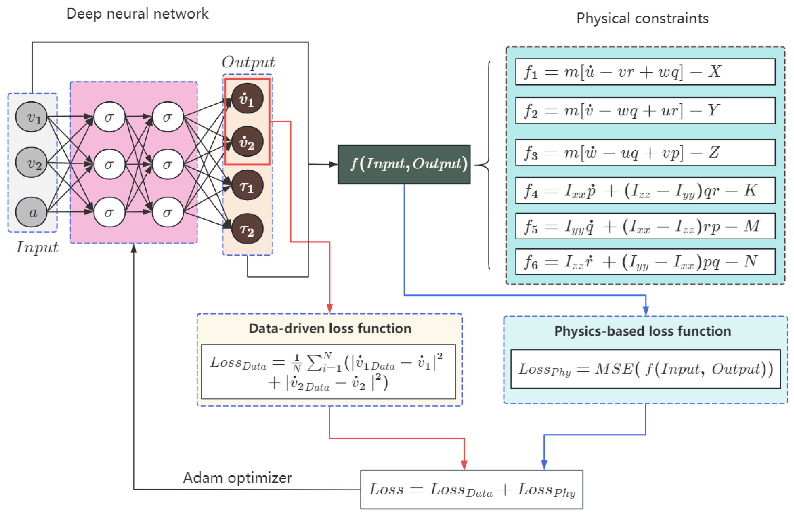
The suggested network, $F_{PINN}$, demonstrated in Figure 2, consists of a fully connected neural network (FCNN). The FCNN is composed of multiple fully connected layers. The input layer $Input=({\mathit{\nu }}_1,{\mathit{\nu }}_2,\mathit{a})$ includes the state variables and control variables of the AUV, with $\mathit{a}={\left[Tx, yite, yitr\right]}^T$, where Tx represents the thrust, $yite$ represents the horizontal rudder, and $yitr$ represents the directional rudder. Thus, the input of the network is a tensor of shape 9 × $N_{batch}$ (where $N_{batch}$ represents the number of data contained in a batch). The output layer $Output=(\dot{{\mathit{\nu }}_1},\dot{{\mathit{\nu }}_2},{\mathit{\tau }}_1,{\mathit{\tau }}_2)$ contains the state change variables and the combined external force/moment. Therefore, the output of the network is a 12 × $N_{batch}$ tensor. The hidden layers use the hyperbolic tangent activation function as typically employed in PINNs [14,15,16], while a linear activation function is utilized in the output layer.

The PINN embeds Equations (8) and (9) into the loss function, thereby achieving a training process constrained by the laws of physics. The loss function for enforcing physical constraints by constructing residual terms is as follows:

$${Loss}_{Phy}=\frac{1}{N_{batch}}\sum _{i=1}^N\sum _{j=1}^6\left({f_j({{\mathit{\nu }}_1}^{\mathit{i}},{{\mathit{\nu }}_2}^{\mathit{i}},{\dot{{\mathit{\nu }}_1}}^{\mathit{i}},{\dot{{\mathit{\nu }}_2}}^{\mathit{i}},{{\mathit{\tau }}_1}^{\mathit{i}},{{\mathit{\tau }}_2}^{\mathit{i}})}^2\right)$$

(12)

where

$$f_1=m(\dot{u}-vr+wq)-X$$

(13)

$$f_2=m(\dot{v}-wq+ur)-Y$$

(14)

$$f_3=m(\dot{w}-uq+vp)-Z$$

(15)

$$f_4=I_{xx}\dot{p}+\left(I_{zz}-I_{yy}\right)qr-K$$

(16)

$$f_5=I_{yy}\dot{q}+\left(I_{xx}-I_{zz}\right)rp-M$$

(17)

$$f_6=I_{zz}\dot{r}+\left(I_{yy}-I_{xx}\right)pq-N$$

(18)

$N_{batch}$ represents the number of training data points in each batch.

The mean square loss function for the data-driven part is as follows:

$${Loss}_{Data}=\frac{1}{N_{batch}}\sum _{i=1}^N{(\left|{\dot{{\mathit{\nu }}_1}}^{\mathit{N}\mathit{e}\mathit{t}}\left({{\mathit{\nu }}_1}^{\mathit{i}},{{\mathit{\nu }}_2}^{\mathit{i}},{\mathit{a}}^{\mathit{i}}\right)-{\dot{{\mathit{\nu }}_1}}^{\mathit{i}}\right|}^2+{\left|{\dot{{\mathit{\nu }}_2}}^{\mathit{N}\mathit{e}\mathit{t}}\left({{\mathit{\nu }}_1}^{\mathit{i}},{{\mathit{\nu }}_2}^{\mathit{i}},{\mathit{a}}^{\mathit{i}}\right)-{\dot{{\mathit{\nu }}_2}}^{\mathit{i}}\right|}^2)$$

(19)

where ${\dot{{\mathit{\nu }}_1}}^{\mathit{N}\mathit{e}\mathit{t}}$ and ${\dot{{\mathit{\nu }}_2}}^{\mathit{N}\mathit{e}\mathit{t}}$ are the network’s predictions, and ${\dot{{\mathit{\nu }}_1}}^{\mathit{i}}$ and ${\dot{{\mathit{\nu }}_2}}^{\mathit{i}}$ are the label values. The total loss function is the sum of the data-driven loss function and the physical constraint loss function:

$$Loss={Loss}_{Data}+{Loss}_{Phy}$$

(20)

Parameter ${\theta }^{*}$ of the PINN is obtained by training by minimizing the loss function with the gradient-based optimizer Adam [18]:

$${\theta }^{*}=arg \underset{{\theta }^{*}}{\min }Loss$$

(21)

To avoid prolonged neural network training time due to differences in the magnitudes of data, as well as inaccurate prediction results caused by gradient vanishing and exploding, the input and output variables are normalized in the calculation process of the physical constraint loss function as follows:

$$\begin{gathered} {\tilde{I}}_{xx,yy,zz}=I_{xx,yy,zz}/\frac{1}{2}\rho L^5, \tilde{m}=m/\frac{1}{2}\rho L^3 \\ \widetilde{{\mathit{\nu }}_1}={\mathit{\nu }}_1/V, \stackrel{~}{\dot{{\mathit{\nu }}_1}}=\dot{{\mathit{\nu }}_1}L/V^2 \\ \widetilde{{\mathit{\nu }}_2}=\widetilde{{\mathit{\nu }}_2}L/V, \stackrel{~}{\dot{{\mathit{\nu }}_2}}=\dot{{\mathit{\nu }}_2}{L}^2/V^2 \end{gathered}$$

(22)

In the formula, $\rho$ represents the fluid density; $L$ denotes the length of the AUV, and $V$ signifies the characteristic velocity.

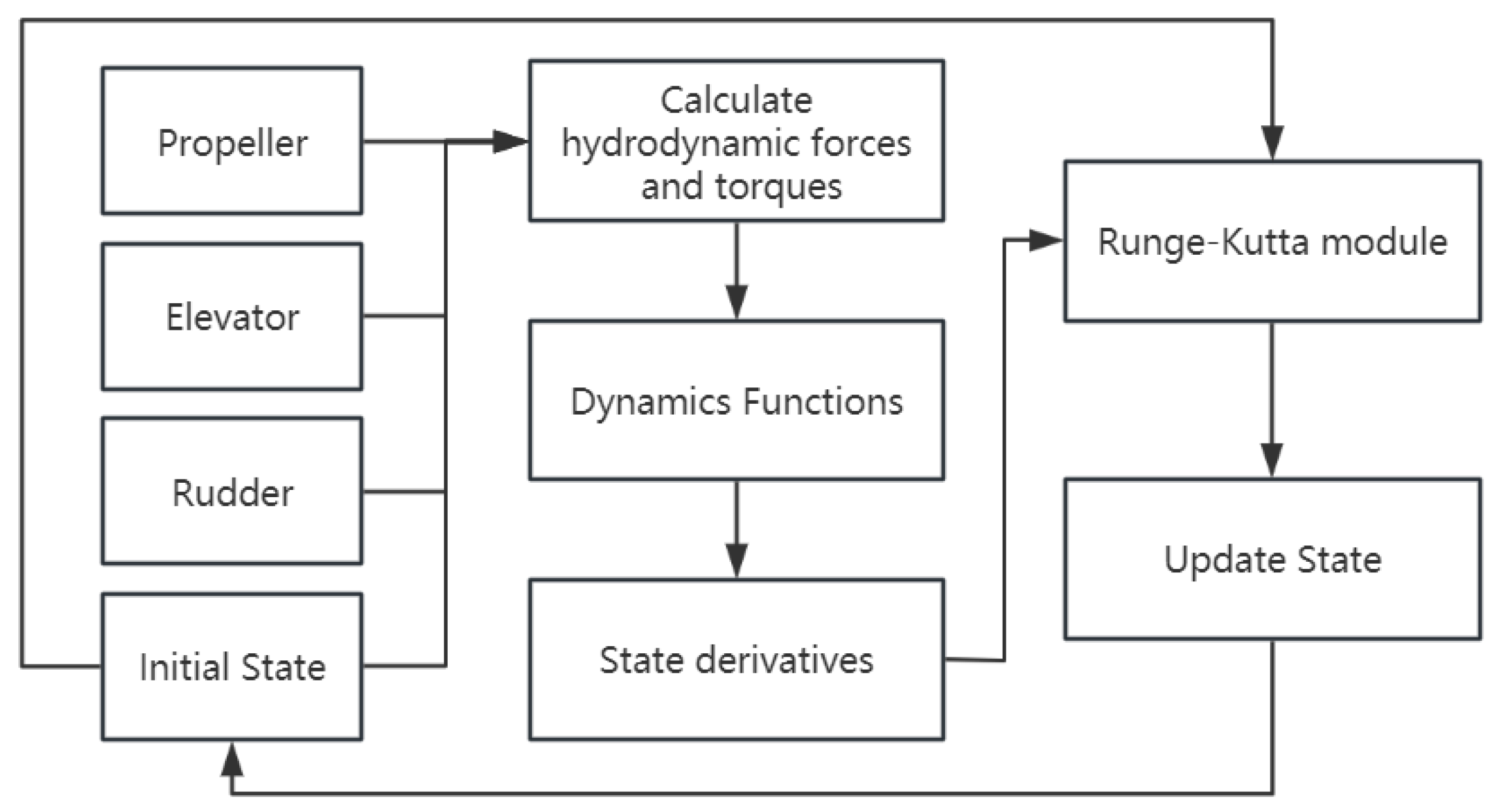
To endow the model with stable, long-term forecasting capabilities, an N-step cyclic iterative training process is proposed, as illustrated in Figure 3. The AUV’s initial state is input into the neural network, which then outputs the corresponding state derivatives and loss function values. Then, the state prediction values for the next time step are obtained by using the 4th-order Runge–Kutta method. These state prediction values, along with the action quantities to be measured, are input into the network, iteratively outputting a total of N times. The network’s gradient is calculated, and gradient descent is executed after computing the weighted average of the cumulative loss function values, as outlined in Algorithm 1.

Algorithm 1: Multi-step iterative training

The training procedure of the model PINN-Net

Input: State values and action values

Result: A set of (sub)optimal network parameters

Step 1: randomly initialize ${\theta }^{*}$

Step 2: while not done do

Step 3: Sample batch of dataset

Step 4:  for all ${batches}_i$ do

Step 5:  Sample N consecutive points $D_j$ from ${batches}_i$

Step 6:   for all $D_j$ do

Step 7:    Calculate the $Loss$ in sequential iterations using $D_j$ in Equation (20)

Step 8:   Calculate the total gradient using $\sum _0^{N-1}Loss\left(D_j\right)$

Step 9:   Update${\theta }^{*}$ with gradient descent

Step 10:    end for

Step 11:  end for

Step 12: end while

2.3. Design of Model Predictive Control Based on PINN

A proficiently trained PINN model can be effectively integrated into model-based control algorithms as a predictive model. In this paper, a trajectory-tracking method combining model predictive control (MPC) and the PINN-based AUV dynamic model is proposed. The MPC algorithm is based on a predictive model to predict the future multi-step states in an open-loop manner and re-optimizes the control variables based on errors in each control cycle. Therefore, the combination of a high-precision model with the MPC algorithm is a natural and logical idea, which can also verify the utility of the PINN model in practical scenarios.

The PINN-based dynamic model of an AUV is defined as

$${\mathbf{S}}_{t+1}=RK\left(F_{PINN}\left({\mathbf{S}}_t,{\mathbf{A}}_t ;{\theta }^{\mathit{*}}\right)\right)$$

(23)

where ${\mathbf{S}}_t$ and ${\mathbf{A}}_t$ represent the state and action at discrete time step t; ${\theta }^{\mathit{*}}$ represents the weights of the network; and RK represents the 4th-order Runge–Kutta numerical integration function, used to integrate the state derivatives obtained by the PINN at each time step.

In the MPC framework, the N-step optimal control problem is represented as

$$\begin{gathered} \underset{\begin{array}{c}{\mathbf{x}}_0,\dots ,{\mathbf{x}}_N\\ {\mathbf{u}}_0,\dots ,{\mathbf{u}}_{N-1}\end{array}}{\min }\frac{1}{2}\sum _{i=0}^N{\tilde{\mathbf{S}}}_i^{\mathrm{T}}{\mathbf{Q}}_{\mathbf{s}}{\tilde{\mathbf{S}}}_i+\frac{1}{2}\sum _{i=0}^{N-1}{\mathbf{A}}_i^{\mathrm{T}}{\mathbf{Q}}_{\mathbf{A}}{\mathbf{A}}_i+\frac{1}{2}\sum _{i=0}^{N-1}{\mathbf{V}}_i^{\mathrm{T}}{\mathbf{Q}}_{\mathbf{v}}{\mathbf{V}}_i \\ s.t. {\mathbf{S}}_{i+1}=RK\left(F_{PINN}\left({\mathbf{S}}_i,{\mathbf{A}}_i ;\mathit{\theta }\right)\right), for i=0,\dots ,N-1 \\ {\mathbf{S}}_0={\widehat{\mathbf{S}}}_0, g({\mathbf{S}}_i,{\mathbf{A}}_i)\le 0 \end{gathered}$$

(24)

where ${\mathbf{Q}}_{\mathbf{S}}$, ${\mathbf{Q}}_{\mathbf{A}}$, and ${\mathbf{Q}}_{\mathbf{V}}$ are positive diagonal weight matrices; ${\tilde{\mathbf{S}}}_i={\mathbf{S}}_{des,i}-{\mathbf{S}}_i$ represents the errors between the true state and the desired state; and ${\mathbf{A}}_i$ and ${\mathbf{V}}_i$ represents the amount of action and the amount of change in action. The initial state is the estimate of the current state, and ${\widehat{\mathbf{S}}}_0$. $g({\mathbf{S}}_i,{\mathbf{A}}_i)\le 0$represents the constraint of state and input, such as actuator or safety restraints. Therefore, the objective function calculates the difference between the predicted state and the reference state within the prediction time step, as well as the energy consumed for control.

Due to the strong nonlinearity and weak interpretability of neural network models, it is difficult to use traditional convex optimization algorithms to solve controllers. Therefore, we adopted a sample-based objective function optimization algorithm, the model predictive path integral algorithm (MPPI) [19,20]. The MPPI algorithm simulates a large number of possible control paths within a predetermined time range by using a system model and then finds the optimal solution by integrating these paths based on the objective function. A significant advantage of this method is that it is not limited by the system model and the type of objective function, making it particularly adaptable to nonlinear systems and unconventional cost functions. Therefore, it is very suitable for MPC optimization problems based on neural network models. The overall control framework flowchart is illustrated in Figure 4.

3. Numerical Experiment

3.1. Simulation Data Acquisition Methods

3.1.1. Simulation Platform

This paper’s numerical simulation experiments are based on a high-precision AUV dynamics simulation platform for data acquisition and the testing of the PINN modeling method. The platform’s AUV prototype features a conventional layout with a cylindrical configuration, as shown in Figure 1. It is equipped with a propeller, a pair of vertical rudders, and a pair of horizontal rudders at the tail. These components are responsible for controlling speed, heading, pitch angle, and depth, respectively. The simulation platform, based on the standard equations of motion for submarine simulation [21], with moderate simplifications, comprehensively considers the 6DOF motion of the AUV in an underwater environment. This includes forward, lateral, and vertical movements, as well as roll, pitch, and yaw. The simulation model’s related hydrodynamic parameters and definitions are shown in

Table 2. Some of the main hydrodynamic coefficients in the AUV simulation platform.

Surge	$X_{\dot{u}}=-0.000418$	$X_u=-0.00574$	$X_{u\left|u\right|}=-0.00188$
Sway	$Y_{\dot{v}}=-0.004584$	$Y_v=-0.01648$	$Y_{v\left|v\right|}=-0.02683$
Heave	$Z_{\dot{w}}=-0.004339$	$Z_w=-0.016897$	$Z_{w\left|w\right|}=-0.09094$
Roll	$K_{\dot{p}}=-0.00584$	$K_p=-0.001914$	$K_{p\left|p\right|}=-0.01241$
Pitch	$M_{\dot{q}}=-0.002042$	$M_q=-0.005209$	$M_{q\left|q\right|}=-0.00251$
Yaw	$N_{\dot{r}}=-0.002061$	$N_r=-0.001832$	$N_{r\left|r\right|}=-0.00281$

, consistently with References [3,21].

In the context of the comprehensive dynamics model of the AUV in the absence of ocean currents, the equation that delineates the forces exerted on the center of mass is outlined as follows [3]:

$$M\dot{v}+C\left(v\right)v+D\left(v\right)v+g\left(\eta \right)=\tau , (\ast )$$

(25)

where M represents the mass matrix with added mass; C(v) indicates the centrifugal and Coriolis matrix; D(v) describes the damping matrix; g(η) represents the restoring force matrix; and τ represents the moments generated by rudders, as well as the forces and torques provided by propellers. Propeller force and moment model are given as follows:

$$T=K_T\rho {\mathrm{D}}^4{n}^2$$

(26)

$$Q=K_Q\rho {\mathrm{D}}^5{n}^2$$

(27)

where D represents the propeller diameter; ρ is the fluid density; $K_T$ and $K_Q$ are the thrust coefficient and the torque coefficient, respectively.

Based on this framework and the hydrodynamic parameters in Table 2, the simulation platform was constructed as depicted in Figure 5. In the simulation platform, the inputs consist of the control variables and the initial state, while the outputs are the state derivatives (in a MIMO structure). The fourth-order Runge–Kutta method is utilized to numerically integrate the state derivatives, given by the Equation (25), and the parameters from Table 2.

3.1.2. Simulation Dataset

The method of collecting training data employed a practical and safety-oriented strategy. It used a PID controller with rough tuning to perform dynamic attitude angle tracking. This method enables the real-time collection of PWM signal values for the propulsion motor and steering servos, along with the corresponding angular acceleration, linear acceleration, linear velocity, and angular velocity data, all while ensuring engineering safety. To meet the practical needs of engineering, both the control signal transmission frequency and the data storage frequency were set to 1 Hz. Our data refresh rate was 20 Hz, which is significantly higher than the control interval. This approach ensures that the stored sensor data are aligned with the control signals, facilitating the online validation of control algorithms. Moreover, this practice ensures the consistency and real-time nature of data collection, providing high-quality and practically valuable data for training neural networks. Consequently, it enables the trained models to better approximate actual engineering requirements and predict the dynamic behavior of the vehicle.

The dataset comprised 20 different trajectories, each spanning a navigation duration of 200 s. The trajectory categories consisted of composite sinusoidal trajectories comprising various frequencies, along with linear and spiral trajectories. All the trajectories involved combinations of various axes, speeds, and accelerations. We uniformly distributed the scale of all data components to ensure that the PINN assigned equal weight to each data component. Ultimately, a set of 10 navigation trajectories was chosen at random for training purposes, while the remaining 10 trajectories were reserved for testing.

3.2. Convergence Experiments

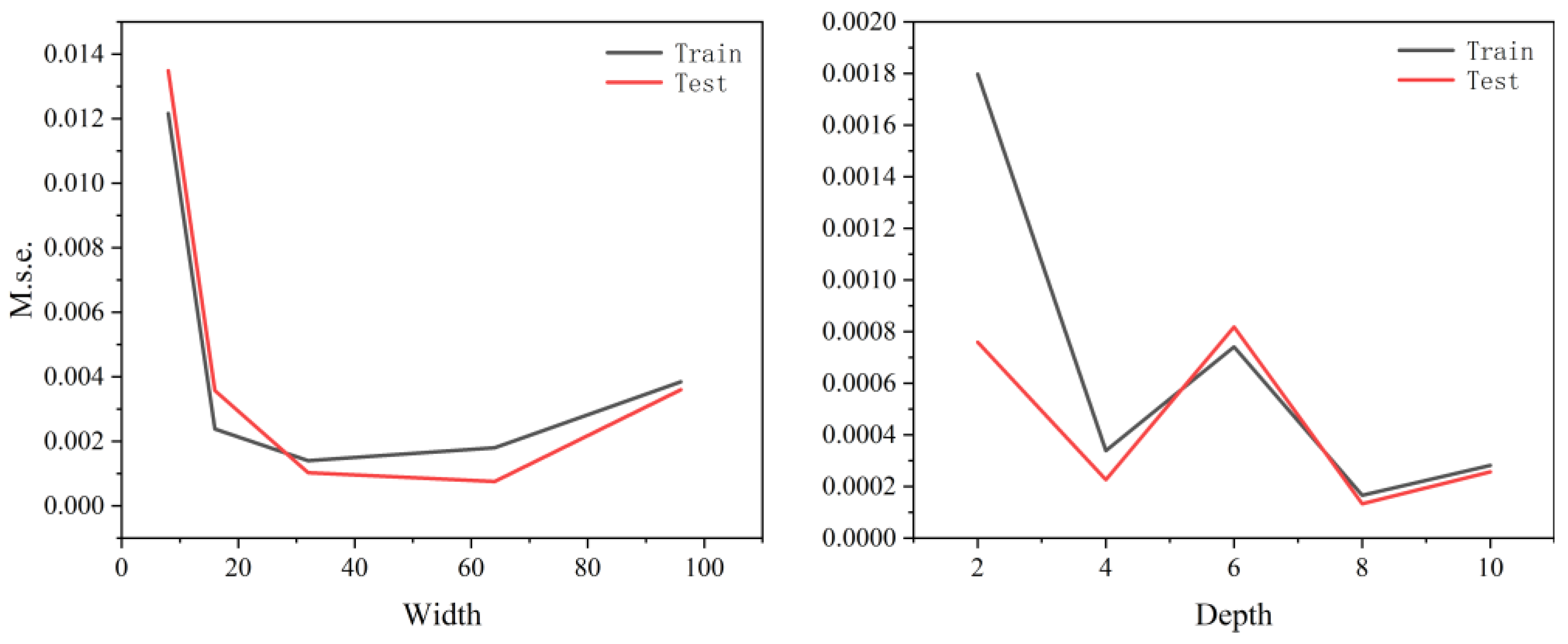
In this section, we will initially illustrate the impact of both the network size and the number of internal iteration steps on the convergence of training for the PINN. For this purpose, we trained the PINN with a time step of 1 s for 2000 epochs. The impact of network size during the training process was evaluated in this experiment. More particularly, we utilized comparative trials to confirm the convergence of training when adjusting the depth and width of the PINN. Figure 6 (on the left) demonstrates the outcomes obtained by altering the width parameter while maintaining a fixed depth of d = 2 layers. We observed that increasing the width from 10 to 64 reduced both training and test errors. However, further increasing the width led to an increase in errors. In addition, Figure 6 (right) illustrates the outcomes obtained by varying the depth parameter while maintaining the width at a constant value of w = 100. It is evident from the results that the optimal configuration, leading to minimized training and test errors, was achieved when the depth was configured to include eight hidden layers.

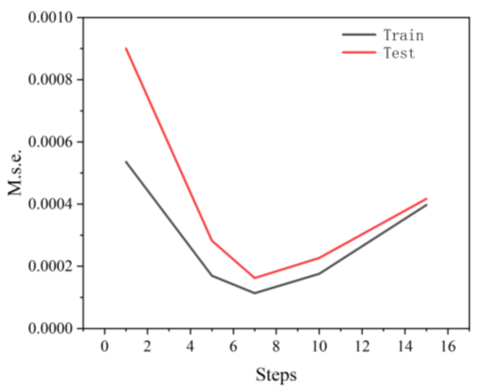
The impact of the number of iteration steps during the training process was also investigated, as presented in this section. More particularly, we utilized the previously validated network size (to mitigate the influence of network size) to confirm the convergence of training when adjusting the number of cyclic iterations in the neural network. Figure 7 illustrates the results when we varied the number of iterations (N) (with fixed dimensions of d = 8 and w = 64). We observed that increasing the number of iteration steps from 1 to 7 reduced the training error. However, further increasing the number of iterations led to an increase in training error. On the other hand, we observed that the test error was minimized when the number of iteration steps was set to n = 7.

3.3. Predictive Performance

We randomly selected trajectories from the test set and input the initial states and rudder angle sequences of each trajectory into the PINN, obtaining long-term motion forecast results for the AUV. We implemented the network architecture as an FCNN with eight hidden layers, each of size 64. Each layer of the network was equipped with a tanh activation function. We trained the PINN on a simulation dataset for 10,000 epochs by using the Adam stochastic gradient descent algorithm, batches of 128 samples, and a constant learning rate of 10⁻⁴. We used mean squared error (MSE) as the evaluation metric to guide the optimization direction of the model. In this study, the PINN was implemented by using the TensorFlow framework. The training process for the models used in the experiments was conducted on a laptop equipped with an Nvidia 3080 graphics card and an Intel i7 CPU.

We utilized the coefficient of determination between the actual values and the predicted values as the evaluation metric:

$$R^2=1-\frac{{\sum }_{i=1}^n{(y_i-{\widehat{y}}_i)}^2}{{\sum }_{i=1}^n{(y_i-{\overline{y}}_i)}^2}$$

(28)

where $y_i$ is the observed value, ${\widehat{y}}_i$ is the predicted value by the model, and ${\overline{y}}_i$ is the mean of the observed data.

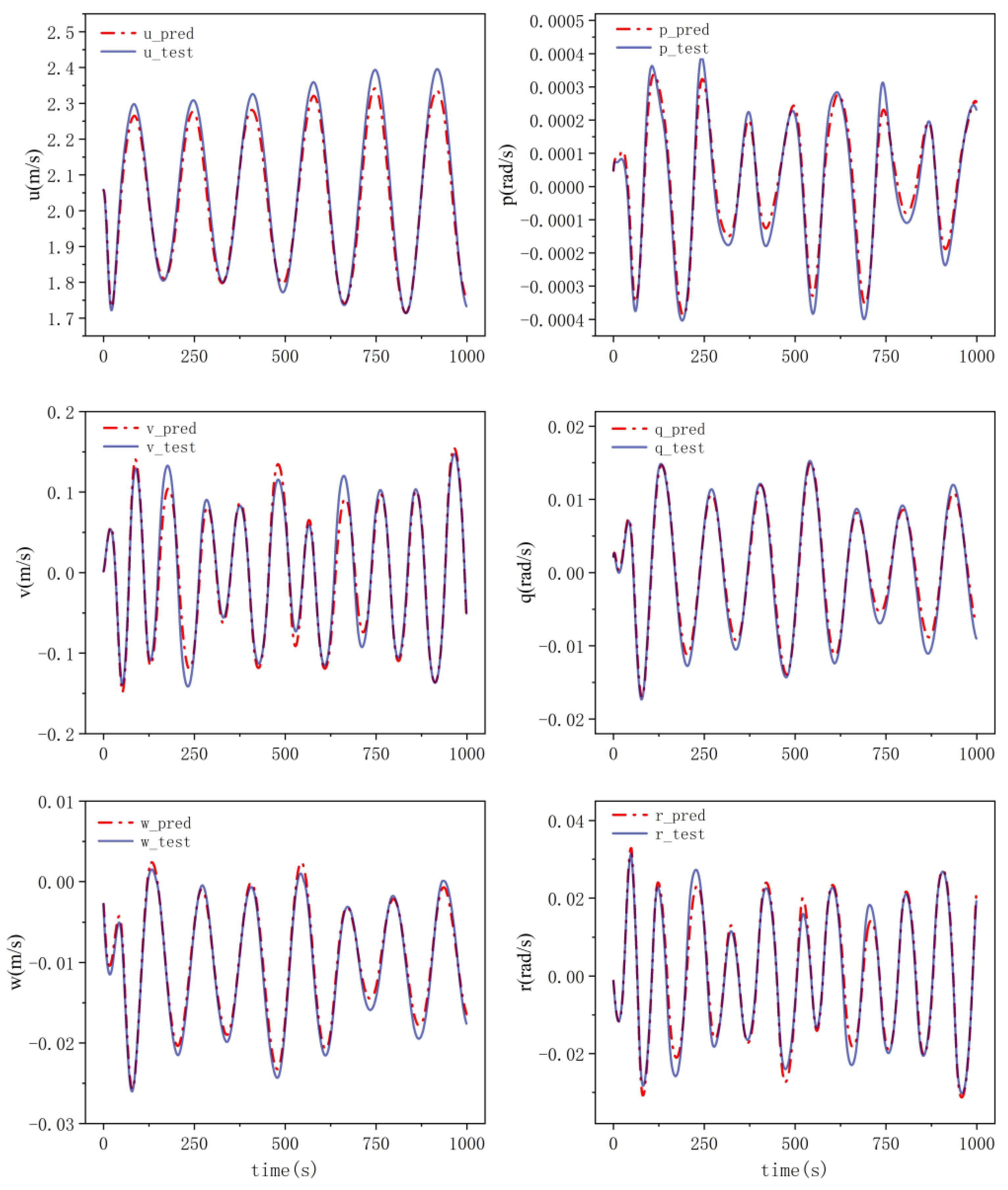
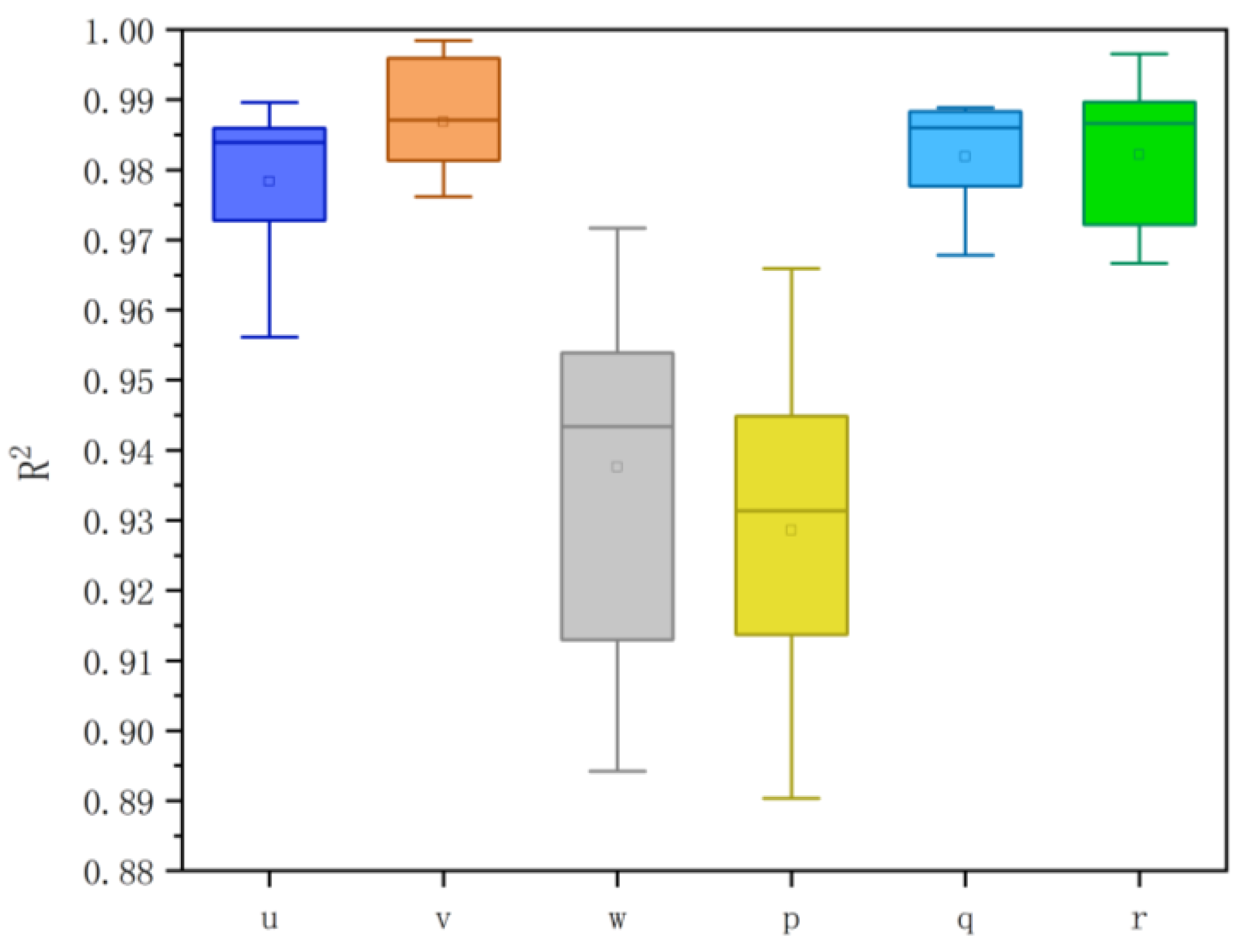
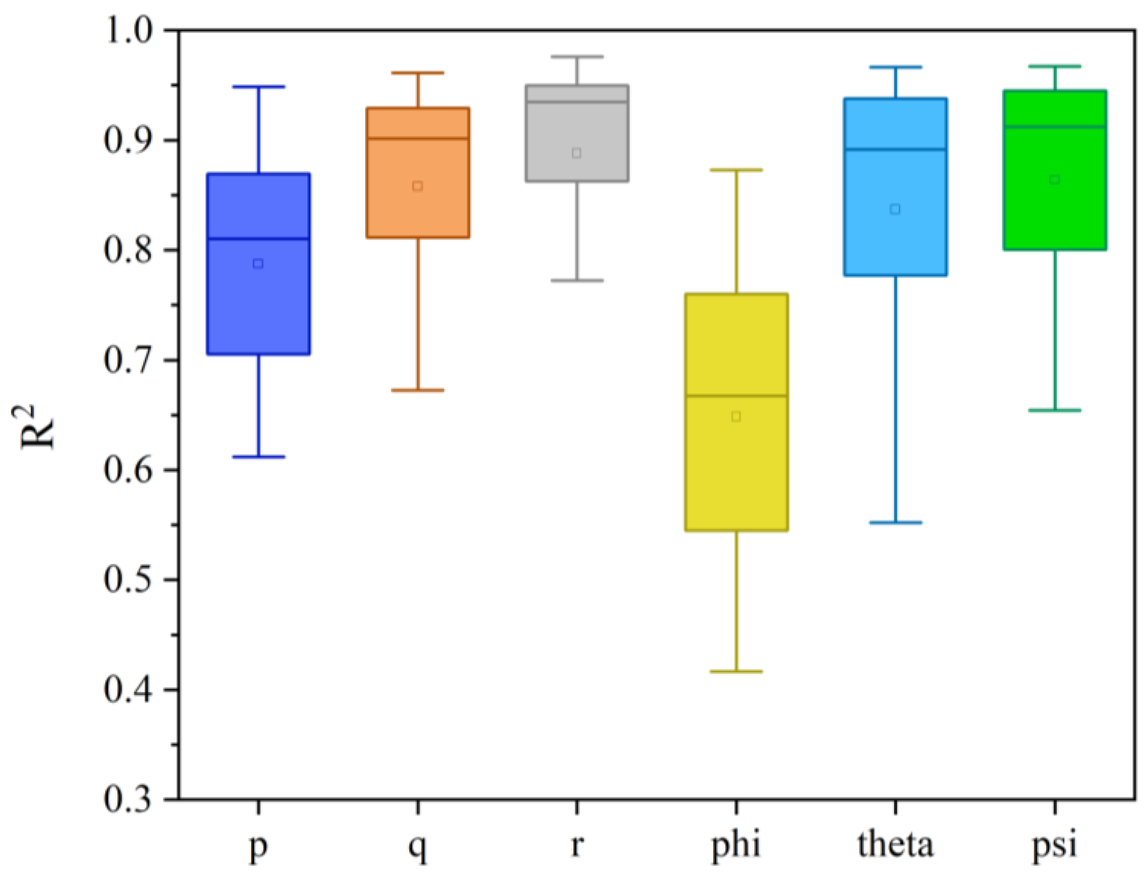
Compared with focusing on reducing errors during the training process, using $R^2$ in the test phase provides a macro-assessment of the model’s performance. $R^2$ measures the degree of correlation between the model’s predictions and the actual values, reflecting the proportion of variance in the predicted results to the total variance. In order to visually demonstrate the predictive performance of the modeling method we proposed, we compared the predictions of the PINN on a test set lasting 1000 s with the ground truth, as illustrated in Figure 8. The experimental data are depicted by the blue line, while the prediction generated by the PINN is illustrated by the red dashed line. The PINN clearly has a strong capability to reconstruct AUV dynamics. Moreover, the PINN also demonstrates strong generalization ability in the test set, accurately predicting unknown trajectories. Significantly, the number of training data available is limited, suggesting the potential to construct a dynamic model of the AUV by utilizing a small dataset and attaining rapid convergence. The statistical results of the model across all test sets are shown in Figure 9. From a statistical perspective, the mean value of the 6DOF fitting coefficients is greater than 0.8, indicating that the PINN model can be well generalized, effectively simulating the AUV motion trajectories.

3.4. Ablation Studies

The PINN incorporates various elements to enhance its predictive accuracy and generalization capabilities. Ablation studies were conducted to evaluate the influence of different network components. Specifically, the studies involved the removal of two key components: (a) the significance of multi-step iterative training and (b) the impact of physics-informed loss on training performance. For all models in the ablation studies, we maintained the same model architecture to ensure a fair comparison. As detailed in

Table 3. Ablation studies.

Multi-Step Iterative Training	PINN-Loss	MSE	${\mathit{R}}^2$
✓	✓	0.0007	0.9152
✓	✗	0.0067	−4.9098
✗	✓	0.0035	0.6153
✗	✗	0.0141	−78.4603

, while each component plays a crucial role, certain components exhibit greater influence than others. Notably, the most substantial contribution stems from the imposition of constraints on network training by the physics-informed loss function. In the absence of this component, errors tend to accumulate significantly for FCNNs that do not integrate physical constraints, leading to divergent prediction outcomes.

3.5. Closed-Loop Trajectory-Tracking Performance

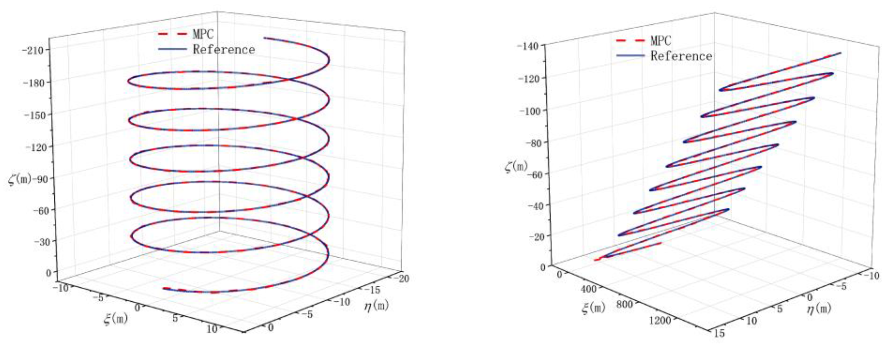
We employed the MPC formulated in Section 2 and the well-trained PINN model to conduct spatial dynamic trajectory-tracking tests on the simulation platform. The MPC controller was developed with Python. The MPC’s prediction horizon was set to 10 time steps, employing the MPPI algorithm with 1000 samples in each control step. To verify the control performance, we designed experiments for tracking three-dimensional helical trajectories and zigzag trajectories. The trajectory-tracking performance results in the simulation environment are shown in Figure 10. The findings indicate that the developed PINN dynamic model can be seamlessly integrated with the MPC algorithm as a predictive model. This MPC-PINN method led to favorable trajectory-tracking outcomes in various scenarios, including steady-state turning and dynamic maneuvering.

4. Field Test

4.1. Experimental Setup

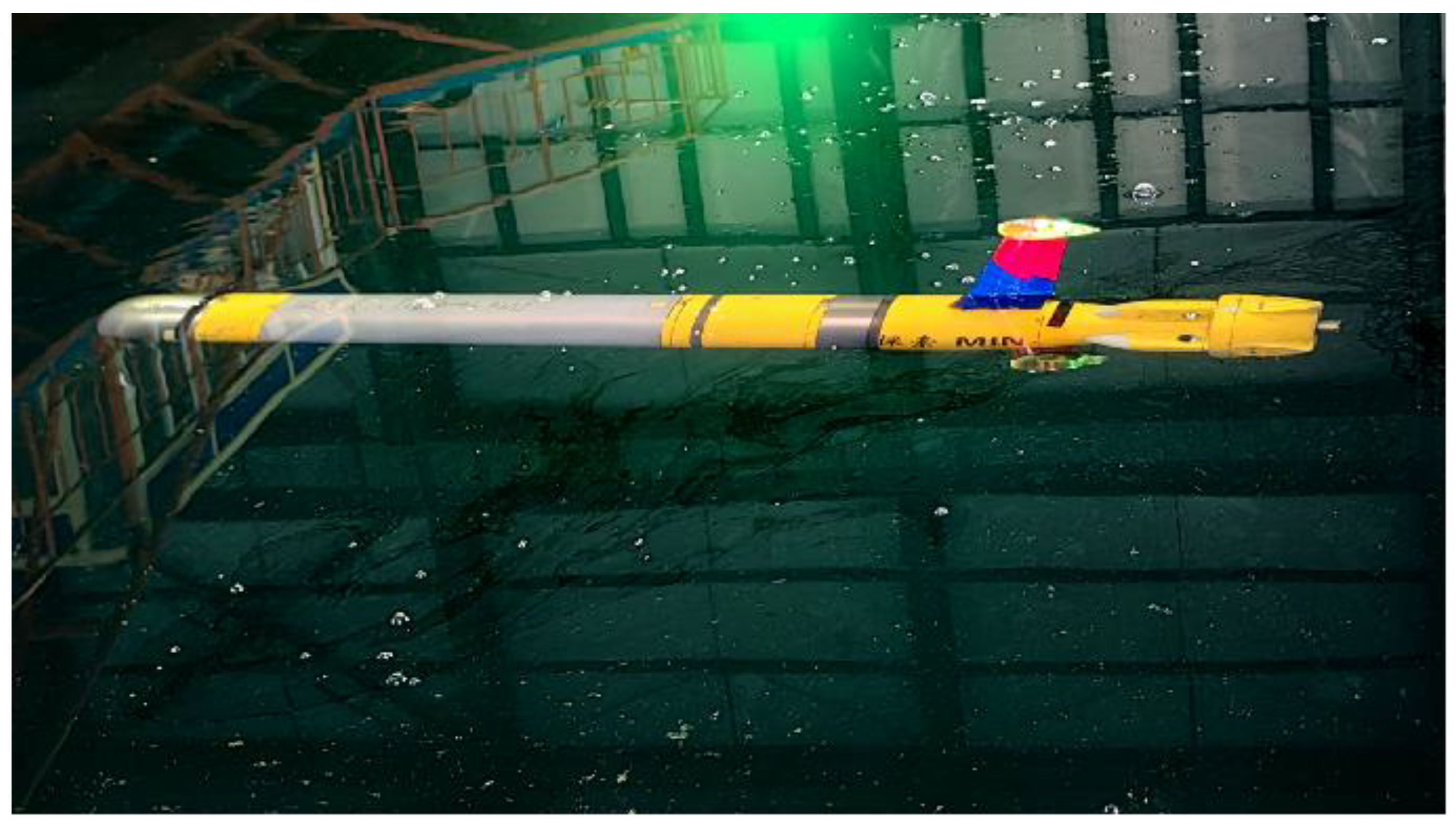
To further evaluate the effectiveness and universality of our method, we utilized a micro-AUV to collect data in a towing tank for modeling and control tests. The actual AUV platform, as depicted in Figure 11, weighed 22.5 kg and was 1.43 m long. The actuators of the system included a main thruster, two vertical rudders, and two horizontal rudders. The sensor equipment consisted of an inertial navigation unit and a depth gauge. The navigation control board utilized Beaglebone Black, equipped with a Jetson Xavier NX module that featured a high-performance GPU for deploying neural network-related algorithms. Limited by sensor accuracy and environmental constraints, in authentic navigational experiments shown in Figure 12, we only tested the modeling effect of the PINN on angular velocity and its application in attitude control. Based on the characteristics of the vehicle and the capabilities of the actuators, we present the relevant constraints for the controller in

Table 4. Related constraint parameters of the controller.

	Unit	Minimum	Maximum	Maximum Rate of Change
Elevator	deg	−40	40	10
Rudder	deg	−40	40	10
Heading angle	deg	−40	−40	5
Pitch angle	deg	−40	10	5
Depth	m	0	12	0.1

, with the control frequency set to 1 Hz.

4.2. Predictive Performance

Similar to the simulation test, we pre-generated multiple sets of sinusoidal excitation targets. This enables the AUV to autonomously execute path-tracking programs by using a simple proportional controller to gather navigational data for the training dataset. To assess the predictive capabilities of the PINN, we intentionally constructed distinct target trajectories during the collection of the test dataset, deviating significantly from the patterns observed in the training dataset. These alternative trajectories may take the form of a ladder curve, a polyline, or a high-frequency sine curve, as shown in the red wireframe in Figure 12. The dataset we ultimately used contained 10 sets of data, each with an average duration of 2 min.

It is worth noting that due to the limited internal space of the micro-AUV, it was not possible to install a Doppler acoustic odometer, and thus we could not obtain linear velocity data. For the PINN that requires complete state input, the unmeasurable variables u, v, and w make it challenging to establish the mapping relationship between network inputs and outputs. In order to test the predictive performance of the PINN under realistic conditions, we removed the unattainable linear velocity terms from the network inputs and eliminated linear acceleration from the output terms. In the simplified PINN used in the field test, the inputs consisted of angular velocity and AUV actions, while the outputs included angular acceleration and torque. Correspondingly, the physics-constrained loss function consisted only of Equations (16)–(18). Based on the simplified PINN model, we tested its predictive performance on AUV attitude, as shown in Figure 13 and Figure 14.

Taking heading angles as an example, the angles were derived by integrating the long-term forecasted angular velocity from the PINN through the utilization of Equation (3), as illustrated in Figure 13. The PINN model, which was trained by using training data derived from tracking sinusoidal trajectories, demonstrates effectiveness in extrapolating to test trajectories that exhibit notable variations. This is evidenced by the strong alignment observed between the model’s predicted outcomes and the corresponding actual values. As illustrated in Figure 14, the coefficient of determination for the PINN model in relation to the angles is predominantly observed to be above 0.64, while for angular velocities, it is primarily distributed above 0.78.

4.3. Attitude Control Performance

To confirm the efficacy of the MPC-PINN approach in practical scenarios, preliminary tests were carried out to evaluate its ability to track reference trajectories. Consistent with the methodology outlined in Section 3.5, the initial phase involved employing the PINN model as the controlled system, with the controller being fine-tuned offline based on predetermined control objectives. Subsequently, the controller was implemented directly on the vehicle for a trajectory-tracking task, with real-time optimization managed through the onboard control system. Constrained by the capacity of the towing tank and the capabilities of the sensors installed on the experimental vehicle, our study focused solely on implementing trajectory-tracking control for the vehicle’s heading and pitch attitudes, as illustrated in Figure 15. The test outcomes indicate that the MPC controller, optimized through PINN tuning, exhibits effective control capabilities, achieving control errors below 1 degree once the AUV reaches stabilization.

5. Conclusions

In this research, the PINN methodology was initially introduced for the purpose of determining the dynamic model of AUVs. Instead of relying solely on data-driven deep learning methods, we employed a physics-driven deep learning method to model AUV dynamics. By embedding the spatial maneuvering motion equations of the AUV into the loss function, we ensured that the network’s predictions are consistent with physical priors. Comprehensive tests were conducted on both a simulation platform and a physical AUV to validate our method. The results demonstrate that the AUV dynamic model established based on the PINN possesses stable and accurate long-term forecasting capabilities, along with good generalization ability. Furthermore, the PINN model can be easily integrated into model-based control algorithms, providing broad prospects in the intelligent control field. In the upcoming research, we are planning to integrate the ocean current disruptions into the model, expanding the applicable scope of the PINN-based AUV dynamics modeling method.

References

1. Zhou, J.; Si, Y.; Chen, Y. A Review of Subsea AUV Technology. J. Mar. Sci. Eng. 2023, 11, 1119. [Google Scholar] [CrossRef]
2. Sathish, K.; Venkata, R.C.; Anbazhagan, R.; Pau, G. Review of Localization and Clustering in USV and AUV for Underwater Wireless Sensor Networks. Telecom 2023, 4, 43–64. [Google Scholar] [CrossRef]
3. Fossen, T.I. Marine Control Systems: Guidance, Navigation and Control of Ships, Rigs and Underwater Vehicles; Marine Cybernetics: Trondheim, Norway, 2002. [Google Scholar]
4. de Barros, E.A.; Pascoal, A.; de Sa, E. Investigation of a method for predicting AUV derivatives. Ocean Eng. 2008, 35, 1627–1636. [Google Scholar] [CrossRef]
5. Fossen, T.I. Models for Ships, Offshore Structures and Underwater Vehicles. In Handbook of Marine Craft Hydrodynamics and Motion Control; John Wiley & Sons, Ltd.: Hoboken, NJ, USA, 2011; pp. 133–186. [Google Scholar]
6. Rehman, F.U.; Huang, L.; Anderlini, E.; Thomas, G. Hydrodynamic Modelling for a Transportation System of Two Unmanned Underwater Vehicles: Semi-Empirical, Numerical and Experimental Analyses. J. Mar. Sci. Eng. 2021, 9, 500. [Google Scholar] [CrossRef]
7. Javanmard, E.; Mansoorzadeh, S. A Computational Fluid Dynamics Investigation on the Drag Coefficient Measurement of an AUV in a Towing Tank. J. Appl. Fluid Mech. 2019, 12, 947–959. [Google Scholar] [CrossRef]
8. Julca Avila, J.; Nishimoto, K.; Mueller Sampaio, C.; Adamowski, J.C. Experimental Investigation of the Hydrodynamic Coefficients of a Remotely Operated Vehicle Using a Planar Motion Mechanism. J. Offshore Mech. Arct. Eng. 2011, 134, 021601. [Google Scholar] [CrossRef]
9. Racine, B.; Paterson, E. CFD-Based Method for Simulation of Marine-Vehicle Maneuvering. In Proceedings of the 35th AIAA Fluid Dynamics Conference and Exhibit, Toronto, ON, Canada, 6–9 June 2005; Fluid Dynamics and Co-located Conferences. American Institute of Aeronautics and Astronautics: Reston, VA, USA, 2005. [Google Scholar]
10. Muñoz, F.; Cervantes-Rojas, J.S.; Valdovinos, J.M.; Sandre-Hernández, O.; Salazar, S.; Romero, H. Dynamic Neural Network-Based Adaptive Tracking Control for an Autonomous Underwater Vehicle Subject to Modeling and Parametric Uncertainties. Appl. Sci. 2021, 11, 2797. [Google Scholar] [CrossRef]
11. Song, S.; Liu, J.; Guo, J.; Wang, J.; Xie, Y.; Cui, J.H. Neural-Network-Based AUV Navigation for Fast-Changing Environments. IEEE Internet Things J. 2020, 7, 9773–9783. [Google Scholar] [CrossRef]
12. Ertogan, M.; Wilson, P.A. Modelling Using Neural Networks and Dynamic Position Control for Unmanned Underwater Vehicles. J. ETA Marit. Sci. 2024, 12, 64–73. [Google Scholar] [CrossRef]
13. Zhang, Y.; Che, J.; Hu, Y.; Cui, J.; Cui, J. Real-Time Ocean Current Compensation for AUV Trajectory Tracking Control Using a Meta-Learning and Self-Adaptation Hybrid Approach. Sensors 2023, 23, 6417. [Google Scholar] [CrossRef] [PubMed]
14. Xu, P.-F.; Han, C.-B.; Cheng, H.-X.; Cheng, C.; Ge, T. A Physics-Informed Neural Network for the Prediction of Unmanned Surface Vehicle Dynamics. J. Mar. Sci. Eng. 2022, 10, 148. [Google Scholar] [CrossRef]
15. Raissi, M.; Perdikaris, P.; Karniadakis, G.E. Physics-informed neural networks: A deep learning framework for solving forward and inverse problems involving nonlinear partial differential equations. J. Comput. Phys. 2019, 378, 686–707. [Google Scholar] [CrossRef]
16. Yang, Z.; Xu, Y.; Jing, J.; Fu, X.; Wang, B.; Ren, H.; Zhang, M.; Sun, T. Investigation of Physics-Informed Neural Networks to Reconstruct a Flow Field with High Resolution. J. Mar. Sci. Eng. 2023, 11, 2045. [Google Scholar] [CrossRef]
17. Karniadakis, G.E.; Kevrekidis, I.G.; Lu, L.; Perdikaris, P.; Wang, S.; Yang, L. Physics-informed machine learning. Nat. Rev. Phys. 2021, 3, 422–440. [Google Scholar] [CrossRef]
18. Kingma, D.P.; Ba, J. Adam: A Method for Stochastic Optimization. arXiv 2014, arXiv:1412.6980. [Google Scholar] [CrossRef]
19. Williams, G.; Aldrich, A.; Theodorou, E.A. Model Predictive Path Integral Control: From Theory to Parallel Computation. J. Guid. Control. Dyn. 2017, 40, 344–357. [Google Scholar] [CrossRef]
20. Williams, G.; Drews, P.; Goldfain, B.; Rehg, J.M.; Theodorou, E.A. Aggressive driving with model predictive path integral control. In Proceedings of the 2016 IEEE International Conference on Robotics and Automation (ICRA), Stockholm, Sweden, 16–21 May 2016; pp. 1433–1440. [Google Scholar]
21. Gertler, M.; Hagen, G.R. Standard Equations of Motion for Submarine Simulation; Naval Ship Research and Development Center: Bethesda, MD, USA, 1967. [Google Scholar]
Figure 1. Coordinate system diagram.
Jmse 12 00801 g001
Figure 2. PINN structure diagram.
Jmse 12 00801 g002
Figure 3. Schematic diagram of multi-step iterative training.
Jmse 12 00801 g003
Figure 4. A flowchart of the overall control framework.
Jmse 12 00801 g004
Figure 5. Schematic diagram of the AUV simulation platform principle.
Jmse 12 00801 g005
Figure 6. The impact of network’s width (left) and depth (right) on convergence.
Jmse 12 00801 g006
Figure 7. The impact of training iteration steps on convergence.
Jmse 12 00801 g007
Figure 8. Observed and predicted values in a test set.
Jmse 12 00801 g008
Figure 9. Distribution of R 2 for prediction results on the test set.
Jmse 12 00801 g009
Figure 10. Trajectory-tracking results.
Jmse 12 00801 g010
Figure 11. (a) Experimental platform. (b) Operating mechanism. (c) Jetson Xavier NX module.
Jmse 12 00801 g011
Figure 12. AUV sailing test in the tank.
Jmse 12 00801 g012
Figure 13. Long-term forecast experimental results in training set (in blue frame) and test set (in red frame).
Jmse 12 00801 g013
Figure 14. Distribution of coefficient of determination for experimental results in test set.
Jmse 12 00801 g014
Figure 15. Results of AUV attitude control tests.
Jmse 12 00801 g015