Abstract
Coral islands and reefs are formed by the cementation of the remains of shallow water reef-building coral polyps and other reef dwelling organisms in tropical oceans. They can be divided into coral islands, coral sandbanks, coral reefs, and coral shoals, of which, Coral shoals are located below the depth datum and are not exposed even at low tide, and sometimes are distributed at water depths exceeding 30 m. Satellite images with wide spatial–temporal coverage have played a crucial role in coral island and reef monitoring, and remote sensing data with multiple platforms, sensors, and spatial and spectral resolutions are employed. However, the accurate detection of coral shoals remains challenging mainly due to the depth effect, that is, coral shoals, especially deeper ones, have very similar spectral characteristics to the sea in optical images. Here, an optical remote sensing detection method is proposed to rapidly and accurately detect the coral shoals using a deep belief network (DBN) from optical satellite imagery. The median filter is used to filter the DBN classification results, and the appropriate filtering window is selected according to the spatial resolution of the optical images. The proposed method demonstrated outstanding performance by validating and comparing the detection results of the Yinli Shoal. Moreover, the expected results are obtained by applying this method to other coral shoals in the Xisha Islands, including the Binmei Shoal, Beibianlang, Zhanhan Shoal, Shanhudong Shoal, and Yongnan Shoal. This detection method is expected to provide the coral shoals’ information rapidly once optical satellite images are available and cloud cover and tropical cyclones are satisfactory. The further integration of the detection results of coral shoals with water depth and other information can effectively ensure the safe navigation of ships.
1. Introduction
Coral islands and reefs are formed by the cementation of the remains of shallow water reef-building coral polyps and other reef-dwelling organisms in tropical oceans [1], which are an extraordinary type of ecosystem in the ocean, known as the “tropical rainforest in the ocean” and the “oasis in the blue desert” [2,3]. They have the highest biodiversity and primary productivity among all marine ecosystems, providing 2.85% of the value and services of the marine ecosystems with only 0.2% of the marine area [4]. Global coral islands and reefs are mainly distributed along the coasts of continents and islands in tropical oceans on both sides of the equator, with the Pacific, Indian, and Atlantic oceans accounting for 55%, 30%, and 15%, respectively [5,6]. At least 96 countries and regions worldwide benefit from coral islands and reefs tourism [7]. Coral islands and reefs can be divided into coral islands, coral sandbanks, coral reefs, and coral shoals. Coral islands and coral sandbanks are both located above the mean high tide level. Coral islands have dense vegetation and are well-developed. However, most coral sandbanks have no vegetation and are unstable. Coral reefs are located between the depth datum and the mean high tide level, exposed at low tide and submerged at high tide. Coral shoals are located below the depth datum and are not exposed even at low tide, and are sometimes distributed at water depths exceeding 30 m. The sketch map of coral islands and reefs is shown in Figure 1.
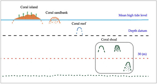
Figure 1.
Sketch map of coral islands and reefs.
Coral islands and reefs are surrounded by coral clusters, with shallow water on the reef beaches, making it difficult for survey ships and surveyors to conduct on-site measurements. In addition, they are widely distributed, making it difficult and inefficient to traverse all of these areas. Therefore, it is not allowed to conduct large-scale and high-frequency on-site investigations in most coral islands and reefs, which are limited by their natural environmental conditions and other factors. Remote sensing has advantages such as large-scale synchronous coverage, the repeated monitoring of the same area, long-term historical archive images, unrestricted regional accessibility, and strong up-to-dateness. In particular, high-resolution remote sensing also has high positioning accuracy. Therefore, remote sensing technology is proven to be an effective technical means for coral islands and reefs monitoring [8,9,10,11,12], and remote sensing data with multiple platforms, sensors, and spatial and spectral resolutions are applied to coral islands and reefs research [13,14,15,16,17,18]. Remote sensing research on coral islands and reefs focuses on analyzing the spatiotemporal dynamic changes of coral islands [19,20,21,22,23,24,25,26,27], evaluating the stability of coral sandbanks [28,29,30], and mapping the geomorphology and habitats of coral reefs [31,32,33,34,35,36,37,38]. However, there are fewer remote sensing studies on coral shoals [39,40], and so this paper takes coral shoals as the study object.
Coral shoals are distributed at a certain depth below the sea surface, and are not usually visible to the naked eye when ships are sailing. Therefore, the areas where coral shoals are distributed are prone to maritime traffic accidents. In order to ensure the safety of ship navigation, it is crucial to mark the accurate location and map the detailed edge shape of coral shoals. In the past, ship surveying was often used for coral shoal investigation, with a limited area and poor timeliness. Moreover, the limitations of the field of view make it difficult to determine the precise boundaries of coral shoals on site. With the continuous development of remote sensing platforms and sensors, the spatial and temporal resolution as well as the detection ability of remote sensing images has been continuously improving. In particular, it is possible to identify the coral shoals on a large scale and detect their edge shape through the comparison of color features between coral shoals and the sea in optical satellite imagery. However, the spectral characteristics of coral shoals and the sea are very similar in optical images because of the depth effect, and so it is not easy to obtain the more accurate information of coral shoals.
In recent years, the emergence and rapid development of deep learning technology have effectively made up for the deficiencies of human-beings in data mining [41,42,43]. Based on sufficient sample datasets, deep learning maximizes the data mining of input information through multi-layer representation, non-linear changes, and feature learning, and has played an important role in remote sensing image classification [44,45]. The deep belief network (DBN) is a widely used deep learning model which was proposed by Hinton et al. in 2006 [41,46]. The DBN combines the advantages of unsupervised learning and supervised learning, improving the effect greatly by training layer by layer. The first application of the DBN in the remote sensing field was Mnih et al., using the DBN to detect roads based on airborne high-resolution images [47]. At present, the DBN is successfully applied to remote sensing classification [48,49,50].
China’s coral islands and reefs account for about 5% of the global total area, mainly distributed in the South China Sea, of which the Xisha Islands are the most representative. Therefore, this paper takes the Xisha Islands as a case study, and the objective is to detect the edge shape of coral shoals with high accuracy using multisource optical imagery by a DBN algorithm. To this end, an optical remote sensing detection method of coral shoals based on the DBN is proposed, taking the Yinli Shoal in the Xisha Islands as the study object. Combining on-site investigation data and the widely used remote sensing classification methods, the validation and comparison of the Yinli Shoal results is carried out to evaluate the detection performance of the proposed method. Further, the optical remote sensing detection method is applied to other coral shoals in the Xisha Islands and the detection results are analyzed comprehensively, so as to evaluate the universality and scalability of the proposed method. Finally, the application of the proposed method is discussed. The location, edge shape, and other information of coral shoals can be obtained quickly and accurately once optical satellite images are available and cloud cover and tropical cyclones are satisfactory, thus providing high-accuracy data support for the safe navigation of ships in coral shoal areas.
2. Materials and Methods
2.1. Study Area
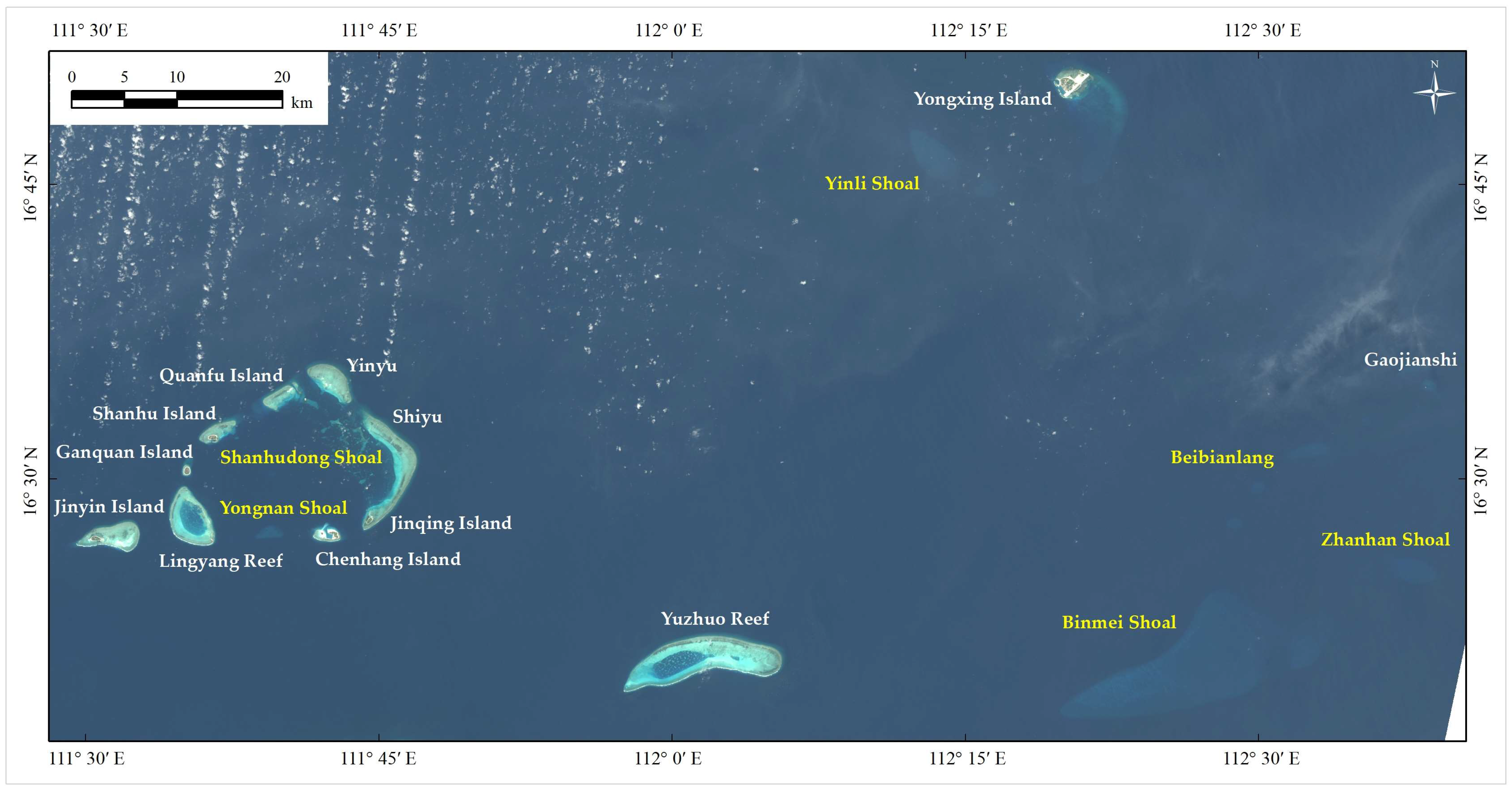
The Xisha Islands are located at the southeast of Hainan Island and the northwest of the vast South China Sea. Centered on Yongxing Island, the capital of Sansha City, they are about 330 km away from Yulin Port in Sanya City and Qinglan Port in Wenchang City. The geographical location of the Xisha Islands is between 15°42′~17°08′ N and 111°10′~112°54′ E, ranging from Bei Reef to Songtao Shoal in the north–south direction and from Xidu Shoal to Zhongjian Island in the east–west direction [1]. According to data records, there are eight independent coral shoals in the Xisha Islands, namely Yinlin Shoal, Xidu Shoal, Binmei Shoal, Beibianlang, Zhanhan Shoal, Songtao Shoal, Shanhudong Shoal, and Yongnan Shoal. The shallowest parts of Yinlin Shoal, Binmei Shoal, Beibianlang, Zhanhan Shoal, Shanhudong Shoal, and Yongnan Shoal have a water depth of over 10 m, while the water depth of Xidu Shoal and Songtao Shoal is above 20 m, with a maximum depth of over 200 m (Figure 2).

Figure 2.
Study area. The yellow text indicates the coral shoals in the Xisha Islands, and the white text indicates the main islands and reefs.
The Xisha Islands have a tropical marine monsoon climate, with a northeast monsoon from November to February and a southwest monsoon from May to August each year. Ocean current and sea wave are influenced by the monsoon and the tidal type is irregular diurnal tide. On average, there are 6~7 tropical cyclones in the Xisha Islands each year, up to more than 10 tropical cyclones, of which 70% originate from the Western Pacific Ocean and 30% from the South China Sea. The peak season for tropical cyclones is concentrated from July to October each year, and there are basically no tropical cyclones from February to March [51].
2.2. Datasets
2.2.1. Optical Satellite Imagery
The selection of satellite images in this study follows two principles. First, there is no cloud cover in the coral shoals studied. Considering the cloudiness of the Xisha Islands, the cloud cover standard of the images is relaxed to 20%, provided that the shoals studied are unaffected. Second, the imaging time of images is avoided before and after TCs and storm surges.
The high-resolution QuickBird, Worldview-2, Worldview-3, SPOT-6, and GF-1 PMS images and medium-resolution GF-1 WFV image are used for coral shoals’ detection. QuickBird image contains 1 panchromatic band with a spatial resolution of 0.61 m and 4 multispectral bands with a spatial resolution of 2.44 m. Worldview-2/3 images contain 1 panchromatic band with a spatial resolution of 0.5 m/0.31 m and 8 multispectral bands with a spatial resolution of 1.8 m/1.24 m. SPOT-6 image contains 1 panchromatic band with a spatial resolution of 1.5 m and 4 multispectral bands with a spatial resolution of 6 m. GF-1 PMS image has 1 panchromatic band with a spatial resolution of 2 m and 4 multispectral bands with a spatial resolution of 8 m, and GF-1 WFV image has 4 multispectral bands with a spatial resolution of 16 m. After selection, the images’ information is listed in Table 1.

Table 1.
Remote sensing images list of coral shoals in the Xisha Islands.
2.2.2. Auxiliary Data
In order to verify and analyze the coral shoals’ information of the Xisha Islands detected in this study, the field data of Yinli Shoal, the tidal data of Yongxing station (Table 1), a nautical chart of the Xisha Islands, an operation map of fishing ground in the South China Sea, and various historical investigation reports are used to provide necessary reference information. In addition, the Tropical Cyclone Best Track dataset proposed by the China Meteorological Administration [52,53] is used to determine whether the tropical cyclones have occurred during the imaging of satellite images used in this study.
2.2.3. Preprocessing of Satellite Images
Data processing mainly includes radiometric calibration, atmospheric correction, and geometric correction. The digital number (DN) value of the pixel is converted into the radiance value on the pupil of the remote sensor using the band offset and gain information in the header file of remote sensing images. Based on the MODTRAN4 + radioactive transfer model [54], an atmospheric correction is carried out to remove the influence of atmospheric scattering and absorption on remote sensing image, and the radiance value of sea surface is calculated. Due to the particularity of the geographical location of the Xisha Islands, it is difficult to measure a large number of ground control points in situ for geometric correction of remote sensing images. Therefore, for QuickBird and Worldview images with high self-location accuracy, no additional geometric correction is carried out, whereas for GF-1 images with slightly poor self-location accuracy, the corresponding QuickBird or Worldview images are used for their geometric correction.
2.3. Methods
2.3.1. DBN Classification Model for Coral Shoals
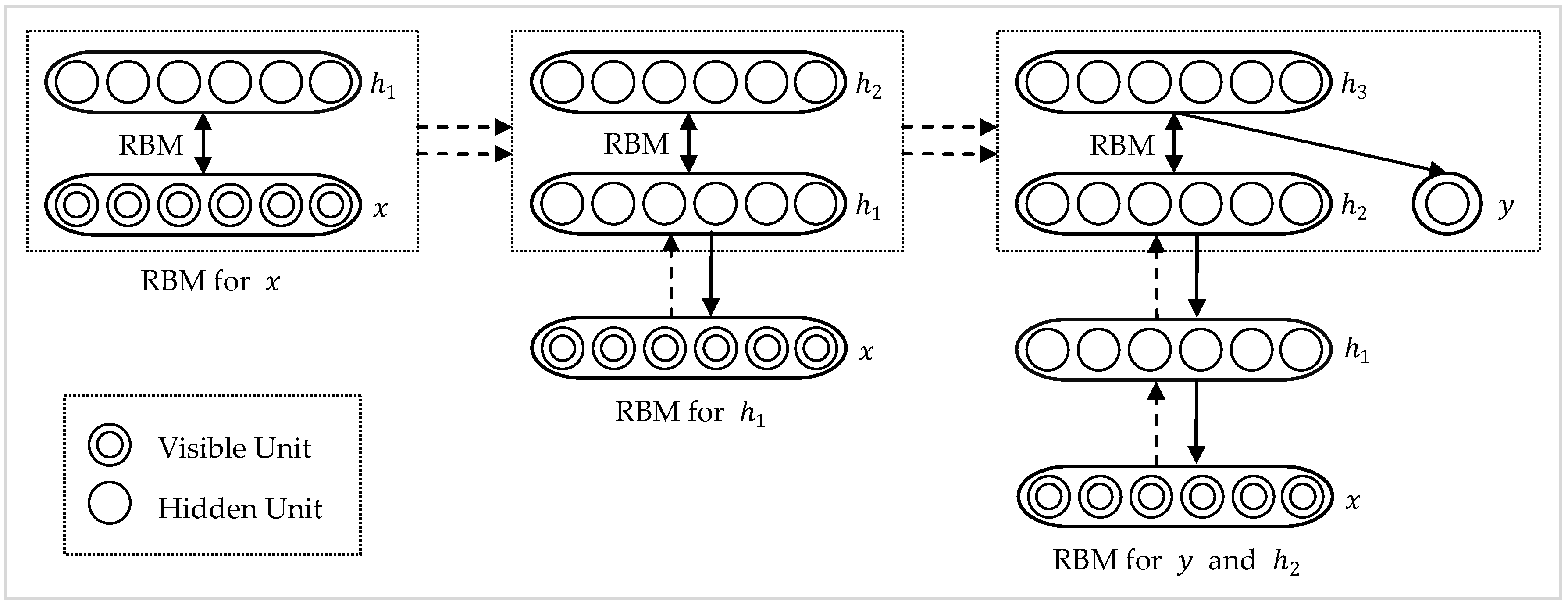
The DBN is a non-convolution model successfully applied in deep frame training, which can be interpreted as a Bayesian probability generation model [41,46]. It is composed of multi-layer random hidden variables. The upper two layers have an undirected symmetric connection, the lower layer obtains a top-down-directed connection from the upper layer, and the state of the lowest unit is the visible input data vector. The DBN is stacked by multiple Restricted Boltzmann Machines (RBMs) [55], as shown in Figure 3. The number of visible neurons in each RBM unit equals the number of hidden neurons in the previous RBM unit. According to the deep learning mechanism, the first layer of RBM units are trained by the input samples and their outputs are used to train the second layer of RBM units. The RBM units are stacked, and the performance of the model is improved by adding layers. In the unsupervised pre-training process, the DBN code is input to the top RBM unit, and then the state of the top unit is decoded to the bottom unit to realize the input reconstruction.
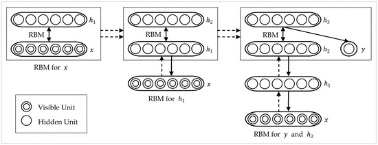
Figure 3.
Generation process of DBN.
Boltzmann machine is a kind of generalized connection, which is used to learn any probability distribution on binary vector [56]. It is a model based on energy. Assuming that the binary random vector , the joint probability distribution is defined by the energy function:
where is the energy function and is the partition function which makes . The energy function of the Boltzmann machine is shown in Equation (2):
where is the weight matrix of the model parameters and is the bias vector.
If the vector is decomposed into two subsets, visible unit and hidden unit , and the image pixels are connected with visible unit , the visible layer composed of the visible unit is used to analyze the input sample pixels, and the hidden layer composed of the hidden unit is used to extract the abstract features of coral shoals and sea as the input of the next layer. The energy function of the joint structure of the visible layer and the hidden layer is as follows:
where , , and are the weight matrix to be trained, and and are the bias vectors to be trained in the visible layer and the hidden layer, respectively. The conditional probability distribution of visible unit and hidden unit is shown in Equations (4)–(6):
where is the activation function.This study uses the Rectified Linear Units (ReLU). The derivative of the ReLU function is:
The ReLU function makes the output of some neurons zero, and the network has certain sparsity and reduces the interdependence between parameters. When and , the problem of gradient saturation will not occur, which accelerates the convergence speed and alleviates the over fitting problem.
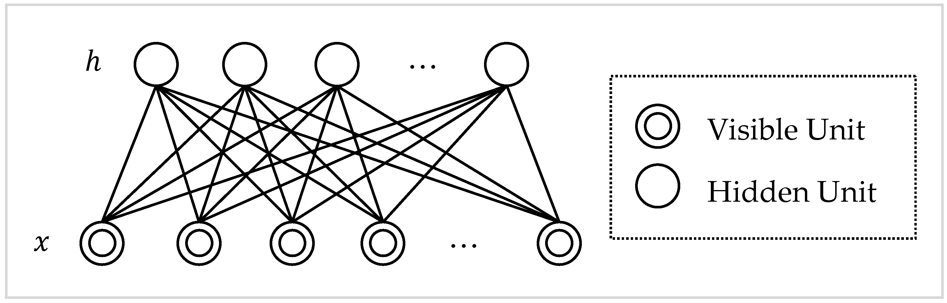
RBM is a special form of Boltzmann machine and the connection between variables is limited. Only visible units and hidden units have connection weights, while there are no connection between visible units and visible units, and between hidden units and hidden units. The undirected graph model of RBM is shown in Figure 4. As the structure unit of DBN, RBM shares parameters with each layer of DBN. The above connection restriction produces excellent properties, that is, independent conditional distribution probability which is easy to calculate:

Figure 4.
Undirected graph model of RBM.
For a binary RBM, the results are as follows:
This enables efficient block of Gibbs sampling and alternates between sampling all hidden units and sampling all visible units at the same time, which makes the RBM training process easier.
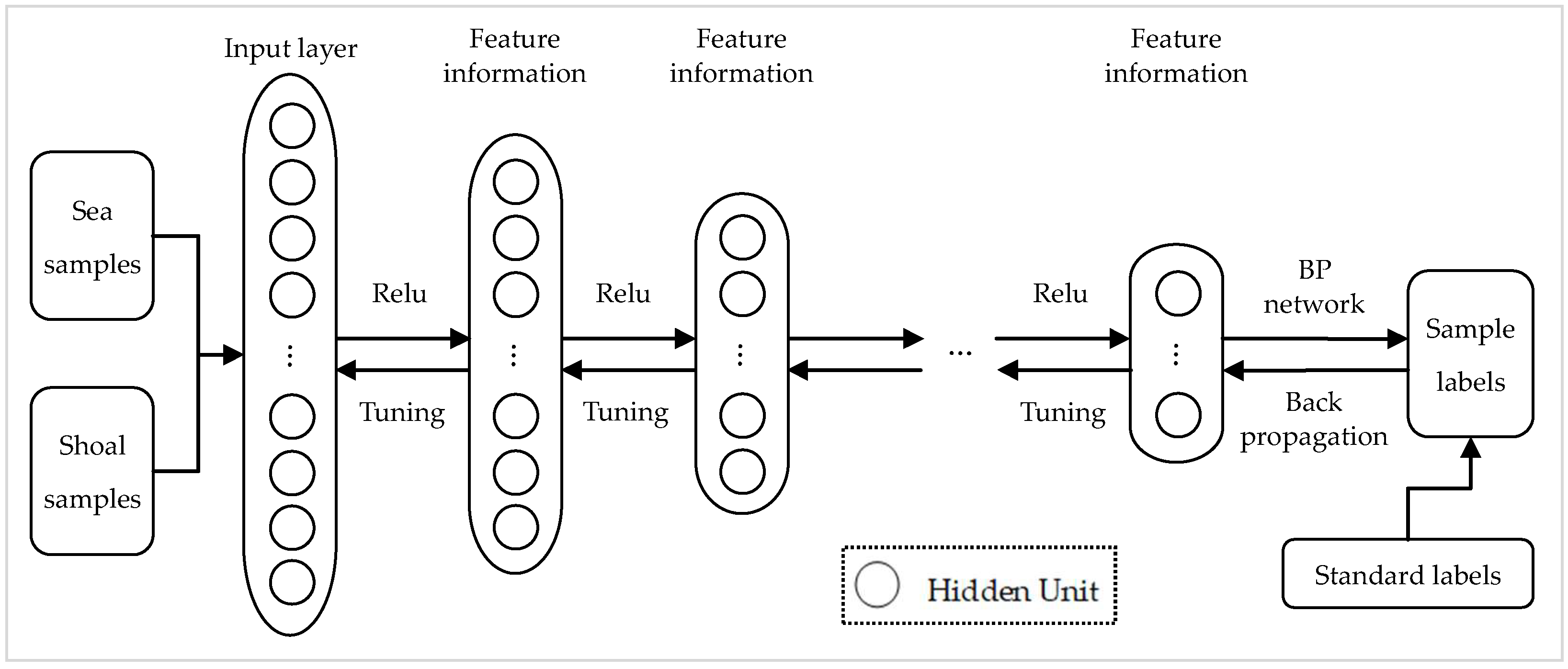
This study establishes a DBN classification model for coral shoals based on optical satellite imagery, consisting of a multi-layer unsupervised RBM network and a layer of supervised back-propagation (BP) network. Firstly, the model pre-training is carried out, that is, unrestrained layer-by-layer training under an unsupervised situation, the lower layer as the input of the upper layer. Then, model fine-tuning is carried out. The BP network of the last layer is trained by the training samples of known standard labels, and the weights of the network are adjusted by the error back propagation layer by layer. In fact, the weights of each layer are trained in advance instead of arbitrary initialization, that is, the reasonable initialization of network parameters replaces the random initialization of BP network weights. Therefore, the network convergence time can be reduced, and then the problem of training time being too long or falling into local minimum can be avoided. DBN is also more effective when the training samples are limited. It improves the model depth through multiple hidden layer nodes, so as to reduce the difficulty of model training caused by insufficient training samples. The DBN classification training model for coral shoals is shown in Figure 5. The regions of interest of known classes are selected to generate the training datasets, which are input into the DBN model mentioned above. Coral shoals and the sea are divided supervised, which provides the binary grid data field for the subsequent edge detection of coral shoals.

Figure 5.
DBN classification training model for coral shoals.
2.3.2. Edge Detection Algorithm GVF-Snake
The edge detection algorithm used in this study is GVF-Snake. Snake refers to the active contour, which is affected by the internal force of the curve itself and the external force calculated from the image, making the curve adapt to the contour of the target object or the characteristics of the image [57,58]. Later, some scholars further proposed the GVF-Snake algorithm, which improved the form of external force, reduced the sensitivity of the algorithm to the initial contour, and stably converged to the concave contour [59].
The GVF-Snake is a deformable parameter curve with a corresponding energy function. To minimize the energy function, the deformation of the parameter curve is controlled, and the parameter curve with the minimum energy is the target contour. The moving process of an active contour is the process of finding the minimum point of energy function. Starting from the initial position, the active contour is deformed by the algorithm, decreasing the energy function until it reaches the edge of the moving target. In the basic snake discrete model, let the snake point of the active contour curve be , , is the number of the snake point, and the energy function with as a variable can be expressed as Equation (12):
where is the internal energy function and is the external energy function. In order to overcome the small capture range of the basic snake model, a gradient vector field is used as the external force to control the contour line approaching the boundary.
The curve is defined, which needs to satisfy the Euler Equation (13) to minimize the energy function when moving in the image plane.
It is the balance equation between the internal force of the curve and the external force controlled by image data.
The GVF vector field is used as the external force field instead of , where Equation (14) is derived.
Then, is defined as the edge potential field of the input image. By minimizing the energy function to achieve the matching between the model and the target contour, the Euler Equation (15) must be satisfied:
where is the Laplacian operator. The stable solution of can be obtained by the variational method and multiple iterations. In this case, the form of external energy is Equation (16):
where is the weight and is the value of the stable solution of at the snake point . By minimizing the external energy, the Snake can be attracted to the edge of the image object.
2.3.3. Optical Remote Sensing Detection Process of Coral Shoals
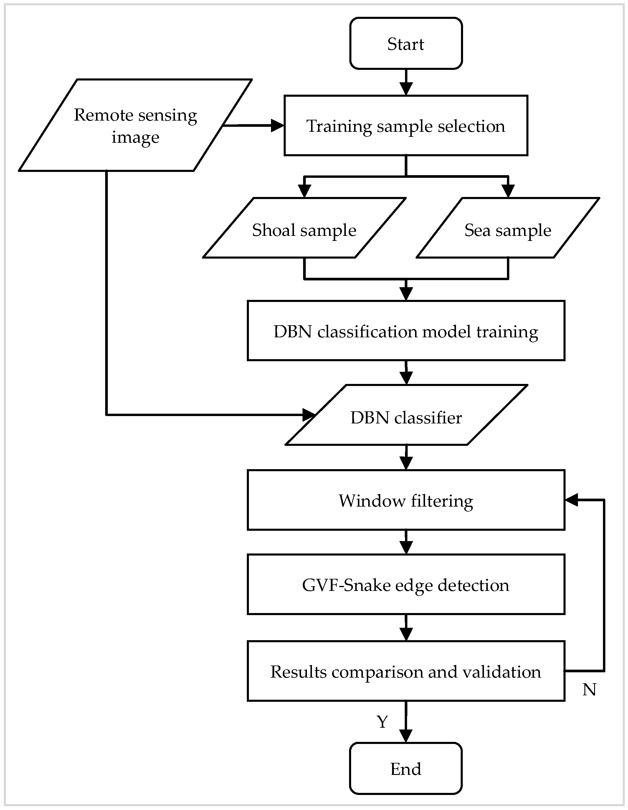
The optical remote sensing detection process of coral shoals in this study is mainly divided into two parts: first, the remote sensing image is classified based on the DBN deep learning model, which is divided into the coral shoals’ area and the sea area; then, the edge detection of the two-classification image is carried out by using the GVF-Snake model. The remote sensing detection flowchart of coral shoals is shown in Figure 6.
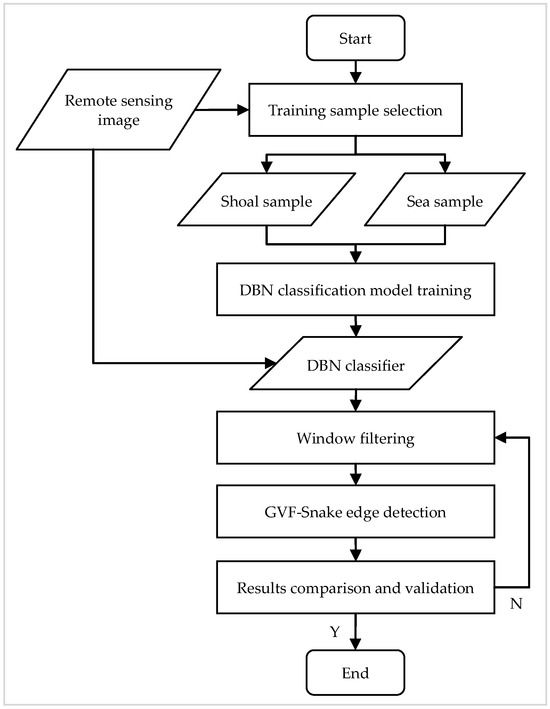
Figure 6.
Flowchart of coral shoals’ remote sensing detection combined DBN with GVF-Snake.
As shown in Figure 6, the optical remote sensing detection process of coral shoals is mainly as follows.
Training sample selection: the coral shoals samples and the sea samples are extracted by means of man–machine intersection to build a classification label sample set by combining the band information and the sample type information, which is used as the input of the DBN classification model.
DBN classification model training: The classification label sample set is input into the DBN model, in which the band information of pixels is input and the type information of samples is output. The unsupervised classification and supervised classification are combined to train the parameters of the DBN network.
Window filtering: the median filter is used to filter the DBN classification results to remove salt-and-pepper noise and smooth the edge of coral shoals.
GVF-Snake edge detection: taking the binary image classified by DBN as the input, GVF-Snake edge detection algorithm is used to extract the edge of coral shoals, and then generate the vector layer of coral shoals.
Results comparison and validation: The classification results of DBN are compared with those of Maximum Likelihood, Support Vector Machine (SVM), and Artificial Neural Network (ANN). The detection results of coral shoals are validated by the field survey data of Yinli Shoal.
3. Results
3.1. Selection of Filter Window Size
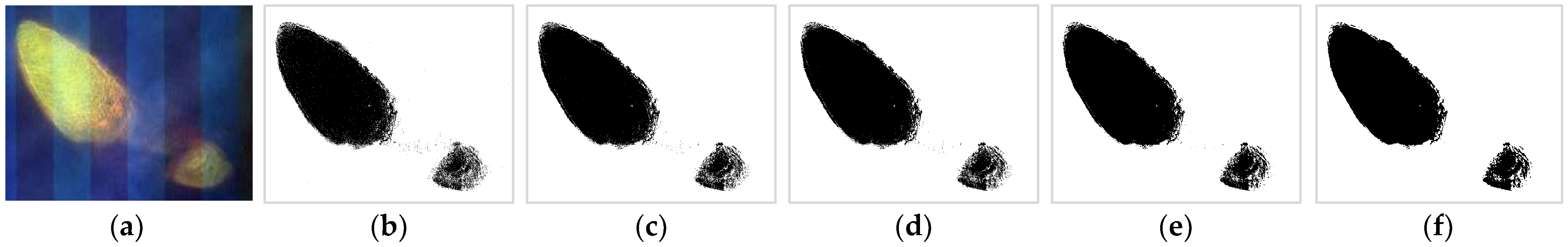
After finishing the DBN classification, it is necessary to filter the classification results further to remove salt-and-pepper noise and smooth the edge of coral shoals. In order to retain more details and suppress the noise effectively, it is essential to select the appropriate filter window size when filtering the DBN classification results. If the window is too large, the filtering efficiency is high, but the details will be lost. If the window is too small, the details will be left, but sometimes the noise will be mistaken for details. Using the eight-band WorldView-3 image with 1.24 m resolution, the four-band SPOT-6 image with 6 m resolution and the four-band GF-1 WFV image with 16 m resolution, the DBN classification results of the Yinli Shoal are filtered by a median filter with a 3 × 3 window, 7 × 7 window, 15 × 15 window, and 27 × 27 window. The filtering results are shown in Figure 7.
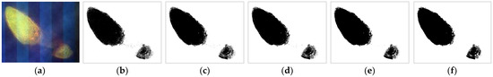
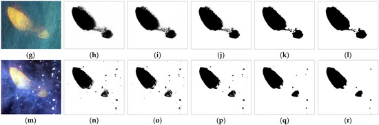
Figure 7.
Enhanced images and their DBN classification and median filtering results of Yinli Shoal: (a,g,m) are enhanced images of Worldview-3, SPOT-6, and GF-1, and the images’ enhancement is to better visualize; (b,h,n) are DBN classification results; (c,i,o) are 3 × 3 window filtering results; (d,j,p) are 7 × 7 window filtering results; (e,k,q) are 15 × 15 window filtering results; and (f,l,r) are 27 × 27 window filtering results.
From the enhanced images and their DBN classification and median filtering results in Figure 7, it can be found that the Worldview-3 image has obvious stripe noise, but it has no significant impact on the DBN classification result. Comparing the filtering results of the 3 × 3 window, 7 × 7 window, 15 × 15 window, and 27 × 27 window, it is more appropriate to select the 7 × 7 window for the median filtering of the Worldview-3 image, which can retain more details of the image. The SPOT-6 image is of good quality and has no obvious noise. For the SPOT-6 image, comparing the median filtering results of the above four window sizes, the filtering effect of the 15 × 15 window is better, which can not only smooth the shoal edge, but also retain the detailed information. There are many scattered cloud noises in the GF-1 WFV image; most of them are distributed in the sea area, and only a few are distributed on the edge of the Yinli Shoal. From the DBN classification results, the clouds are identified as coral shoals, but the cloud noises are effectively removed by the median filter. The median filtering results of the four window sizes showed that the 15 × 15 window is more suitable for the GF-1 WFV image, which can suppress most of the cloud noises and better identify the contour information of the coral shoals. Therefore, the 7 × 7 window is selected to filter the DBN classification results for the Worldview-3 and other remote sensing images with a spatial resolution of 1-2 m, and the 15 × 15 window is selected for the SPOT-6, GF-1 WFV, and other remote sensing images with a spatial resolution of a meter level and more than ten meters.
3.2. Detection Results’ Validation and Comparison of Yinli Shoal
Combining on-site investigation data and widely used remote sensing classification methods, the validation and comparison of the Yinli Shoal detection results are carried out to evaluate the detection performance of the proposed method.
3.2.1. Results Analysis and Validation
Based on the Worldview-3, SPOT-6, and GF-1 WFV images, the detection results of the Yinli Shoal are obtained by DBN classification combined with the GVF-Snake edge detection algorithm, as shown in Figure 8. After a comprehensive analysis of the detection results, the Yinli Shoal is distributed in northwest–southeast direction and its area is about 20 km2. The length from northwest to southeast is about 10 km, and the widest part from northeast to southwest is about 3 km. The Yinli Shoal is divided into northwest and southeast parts. The northwest part has a large area and a shallow water depth, and the shallowest part is about 10 m. The southeast part has a small area and a water depth of more than 14 m. The area between the northwest and southeast is deeper. Due to the limitation of the imaging ability of the optical remote sensing images, the edge of the shoal range in this area is not clear, and the image characteristics on different images are slightly different, which leads to a great difference in the detection results on the different images.
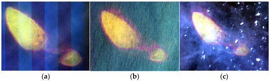
Figure 8.
Detection results of Yinli Shoal based on (a) Worldview-3, (b) SPOT-6, and (c) GF-1 WFV.
Supported by the relevant projects, the field data in some areas of the Yinli Shoal were measured. With the aid of these data, combined with a nautical chart of the Xisha Islands, the spatial distribution range of the Yinli Shoal is extracted by man–computer intersection interpretation based on the high-resolution optical remote sensing images. This interpretation result is used as the standard data to validate the DBN detection results. A comparison between the three detection results and the interpretation result is shown in Figure 9.
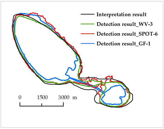
Figure 9.
Comparison between the detection results and the interpretation result of Yinli Shoal.
The interpretation result is divided into 10 equal parts randomly, and 10 profiles are made along the vertical direction of the interpretation result, whose distribution is shown in Figure 10. The distance between the interpretation and detection results on the profile are calculated respectively, and their absolute values are used to evaluate the accuracy of the detection results, as shown in Table 2. It can be seen that the accuracy of the detection results is closely related to the spatial resolution and image quality of the remote sensing images. For the Worldview-3 image, the edge of the Yinli Shoal is well detected. Except for the area between the northwest and southeast, which is quite different from the interpretation results, there is a small area missing in the southeast. For the SPOT-6 image, a greater level of detection exists on the northeast side of the northwest part, and it is found that there are easily mixed image features in this area. The detection result of the GF-1 WFV image shows that its effect is poor, and the edge is relatively coarse, especially in the area between the two parts. There may be two reasons: first, because of the low spatial resolution of the GF-1 WFV image, the image characteristics of the shoal are not obvious; second, because of the large amount of clouds in the image, the shoal details are filtered out in the median filtering in order to suppress most of the clouds.
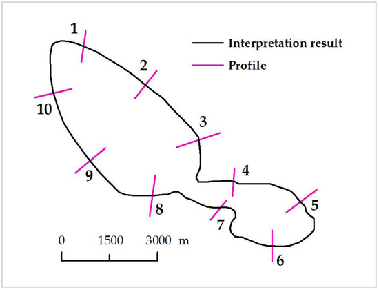
Figure 10.
Profiles’ distribution for accuracy evaluation of Yinli Shoal detection results.
Table 2.
Accuracy of Yinli Shoal detection results (Unit: m).
Comparing the remote sensing detection results and the interpretation results of the Yinli Shoal, it can be found that the DBN detection results are more detailed and more precise than the interpretation results in the edge description of the coral shoals. The appropriate manual correction based on the DBN detection results of the coral shoals can replace the tedious process of manually mapping the edge of coral shoals, which is of great significance in obtaining coral shoal information on a large scale in the South China Sea.
3.2.2. Results Comparison
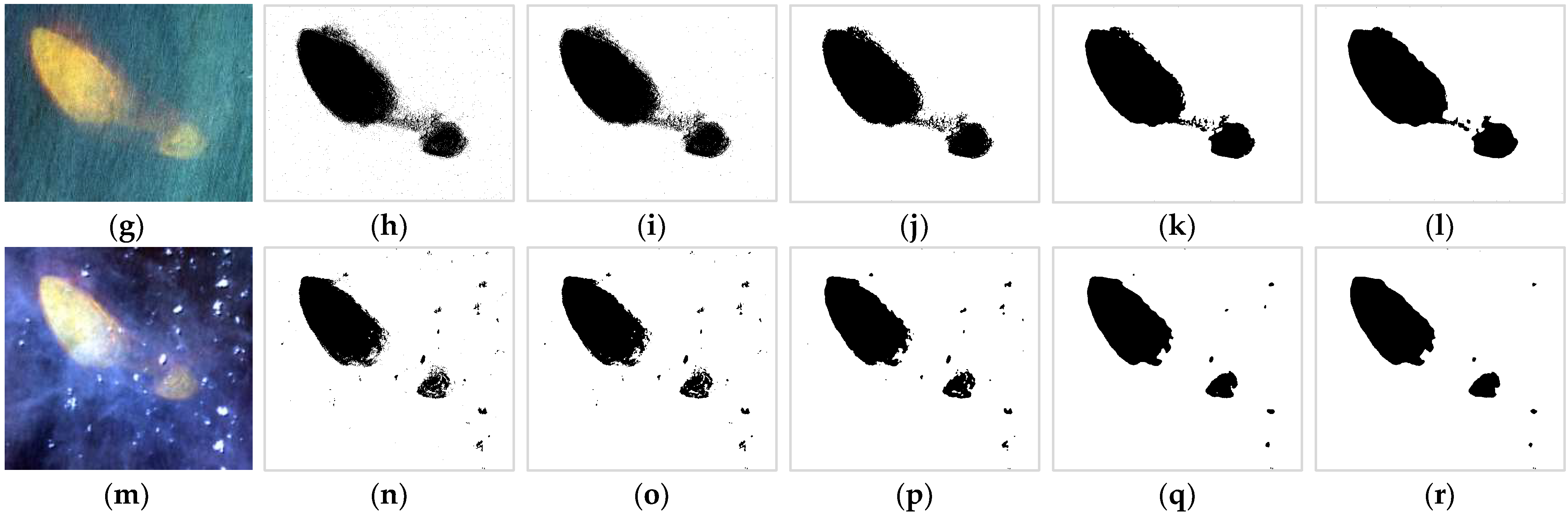
The detection results of the DBN are compared with those of the Maximum Likelihood, SVM, and ANN. Maximum Likelihood, SVM, and ANN are widely used supervised classification methods with high accuracy. Maximum Likelihood is a simple, fast, and robust classifier, which has been applied to many fields [60]. Among various classification methods, ANN is the best in terms of accuracy, but it needs more training samples [61], while SVM has good resistance to the number and purity of training samples [62,63].
Based on the SPOT-6 4-band multispectral image of the Yinli Shoal with the best image quality, using the same training sample data, Maximum Likelihood, SVM, and ANN are used for image classification, respectively, and then the 15 × 15 window median filtering and GVF-Snake edge detection are performed. The detection results of the Yinli Shoal using different classification methods are shown in Figure 11. It can be seen that the detection results based on the Maximum Likelihood classification are poor, and the detection results based on the SVM and ANN classification are equivalent to those based on the DBN classification. Affected by the characteristics of remote sensing images, there is a higher level of detection on the northeast side of the northwest part, and in comparison, the DBN classification method has higher detection accuracy here. However, the detection results based on the SVM and ANN classification are closer to the interpretation results in the deeper area between the northwest and southeast parts of the Yinli Shoal, which are better than those based on the DBN classification.

Figure 11.
Detection results of Yinli Shoal using different classification methods.
3.3. Detection Results’ Analysis of Coral Shoals in the Xisha Islands
The optical remote sensing detection method is applied to other coral shoals in the Xisha Islands and the detection results are analyzed comprehensively to evaluate the universality and scalability of the proposed method. Among eight coral shoals in the Xisha Islands, the Xidu Shoal and Songtao Shoal could not be identified due to the limitation of the remote sensing image detection capability. The distribution area of the Shanhudong Shoal and Yongnan Shoal is relatively small, so the high-resolution QuickBird, Worldview-2, and GF-1 PMS images are used for the detection of these two shoals. At the same time, multi-temporal optical images are used to analyze the changes in the coral shoals. For the Binmei Shoal, Beibianlang, and Zhanhan Shoal with large areas, the moderate-resolution remote sensing images are suitable, the Chinese GF-1 WFV images are selected in this study, and the Landsat and Sentinel images can also be used to achieve the same effect.
Using the above images, the detection results of the coral shoals in the Xisha Islands are obtained based on the optical remote sensing detection method for the coral shoals proposed in this study. According to the analysis and evaluation results of the Yinli Shoal, the DBN classification results of the Binmei Shoal, Beibianlang, and Zhanhan Shoal are filtered by the 15 × 15 window, and the DBN classification results of the Shanhudong Shoal and Yongnan Shoal are filtered by the 7 × 7 window.
On the basis of the remote sensing detection results, the basic information of coral shoals in the Xisha Islands is analyzed comprehensively. The Binmei Shoal is about 24 km east of the Yuzhuo reef, covering an area of about 130 km2. It is distributed in the northeast–southwest direction, with a length of about 26 km from northeast to southwest. It is narrow at both ends and wide in the middle. The widest part is about 10 km and the narrowest part is less than 2 km. Beibianlang is about 6 km north of the Binmei Shoal, composed of three oval underwater reefs with a total area of about 5.1 km2. The Zhanhan Shoal is located about 7 km northeast of the Binmei Shoal, with an area of about 6.4 km2. It is roughly oval in shape, about 3.3 km long from northwest to southeast, and about 2.0 km wide from northeast to southwest. The Shanhudong Shoal is located about 1 km east of Shanhu Island, with a small area of only 0.05 km2. It is distributed in a northeast–southwest oval shape, and is about 370 m long and 170 m wide. The Yongnan Shoal is located between the Lingyang reef and Guangjin Island, covering an area of about 2.4 km2. It is distributed in a semicircle in an east–west direction, with a length of about 2.5 km in the east–west direction and a width of about 1.2 km in the south–north direction. Comparing the four temporal detection results of the Shanhudong Shoal and Yongnan Shoal, it is found that there is no obvious change in the two shoals from 2005 (or 2006) to 2018, which may be due to the fact that coral shoals are distributed at a certain depth below the sea surface and are less affected by human activities and global climate change.
4. Discussion
4.1. Comparison of Edge Detection Results between GVF-Snake and Traditional Operators
In order to evaluate the edge detection effect of the GVF-Snake algorithm, the Sobel operator, Laplace of Gauss (LOG) operator, and Canny operator are selected to compare their edge detection results with those of GVF-Snake. Sobel and LOG are differential-based operators, which use the first or second derivative of the pixel grey values in an image to obtain the extreme value at the place where the grey values change rapidly for detection. Sobel is a first-derivative operator that is easy to implement. Due to the neighborhood weighted average before the differential calculation, the Sobel operator has a strong ability to suppress noise, but the detected edge is coarser. LOG is a second-derivative operator, and its detection results are closely related to the window size. In different spatial resolution images, the detection is carried out with different window sizes, and the edges with different details can be obtained. Using a small window can obtain more image details, but it is also sensitive to noise, while using a large window is not sensitive to noise, but it will ignore the image details. Canny is a non-differential operator, which is a multi-level edge detection algorithm. Its advantages are a low error rate, high localization, and a single edge response.
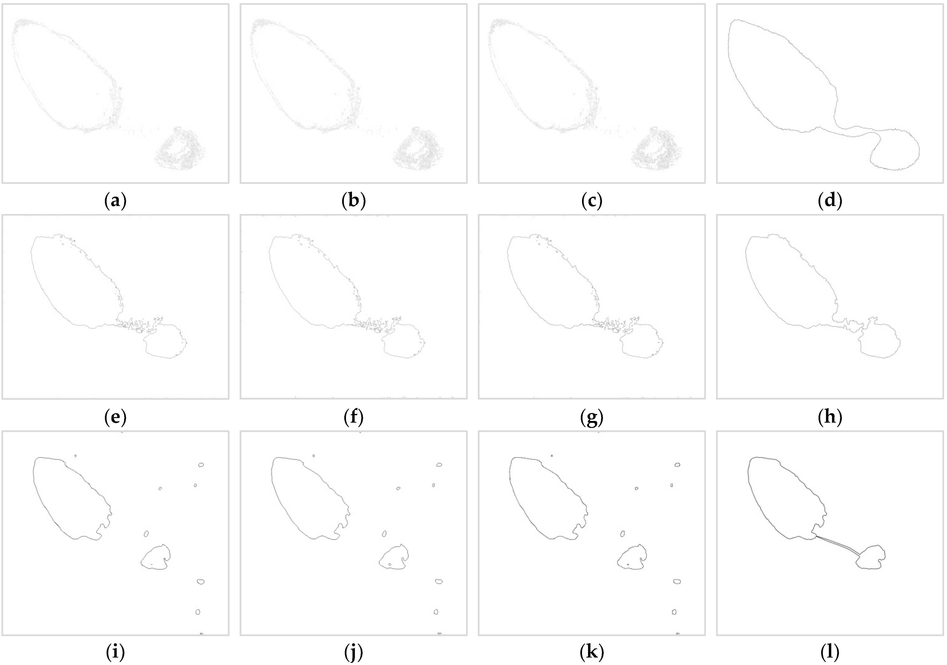
Based on the 7 × 7 window filtering results of the DBN classification of the Worldview-3 images and the 15 × 15 window filtering results of the DBN classification of the SPOT-6 and GF-1 WFV images, the edge detection of the Yinli Shoal is carried out using the Sobel operator, LOG operator, Canny operator, and GVF-Snake algorithm, respectively. The results are shown in Figure 12.
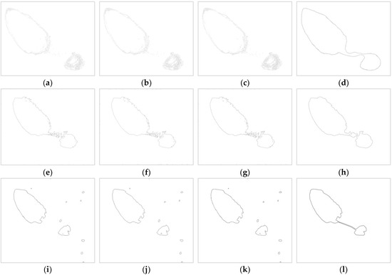
Figure 12.
Edge detection results of Yinli Shoal based on 7 × 7 window filtering results of Worldview-3 and 15 × 15 window filtering results of SPOT-6 and GF-1: (a,e,i) using Sobel operator; (b,f,j) using LOG operator; (c,g,k) using Canny operator; and (d,h,l) using GVF-Snake algorithm.
As shown in Figure 12, the edge detection effect of the four algorithms is affected by the DBN classification results, and the detail richness of the classification results is directly related to the final detection results of coral shoal. Due to the high spatial resolution of the Worldview-3 image, its DBN classification results are rich in details, and so the edge of the Yinli Shoal is described in detail after edge detection, while the resolution of the GF-1 WFV image is slightly lower, and the detected edge of the coral shoals is coarser. On the whole, the GVF-Snake can better obtain the overall edge of the Yinli Shoal, which is most in line with the expectations. However, the GVF-Snake has higher requirements for the initial contour, and the shape structure and location of the initial contour have a greater impact on the final detection results.
4.2. Influence of the Spatial and Spectral Resolution of Remote Sensing Images on the Coral Shoal Detection Results
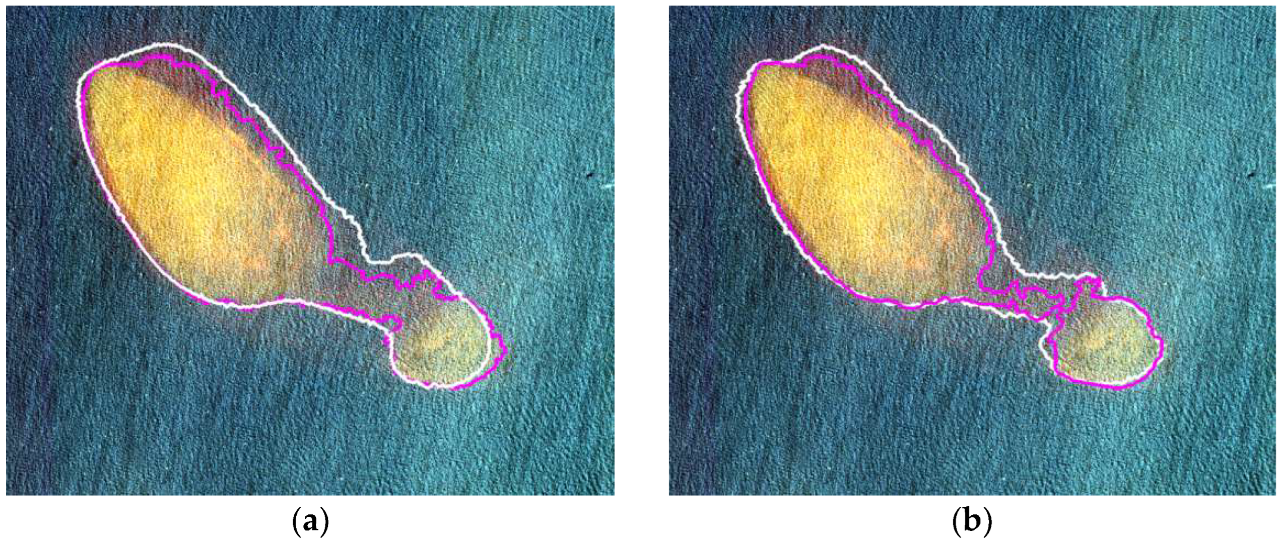
As mentioned above, multi-source remote sensing images with different spatial resolutions greatly impact the detection results of coral shoals. The detection results of the Yinli Shoal based on WorldView-3 and SPOT-6 are obviously better than those based on GF-1 WFV. The Yinli Shoal results in Figure 8 are obtained based on the multispectral images of Worldview-3 and SPOT-6. Worldview-3 and SPOT-6 also have panchromatic bands, and Panchromatic and multispectral image fusion can also improve the spatial resolution of the images. Considering that the spatial resolution of the Worldview-3 multispectral image is very high, reaching 1.24 m, this study uses the SPOT-6 image to analyze the accuracy change of the detection results of the coral shoals by panchromatic and multispectral image fusion. The results of the Yinli Shoal with the 7 × 7 window and the 15 × 15 window are shown in Figure 13. It can be found that although panchromatic and multispectral image fusion improves the spatial resolution of the image, it also has a certain impact on the spectral characteristics of the image, which makes the detection results worse.
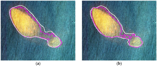
Figure 13.
Detection results of Yinli Shoal based on SPOT-6 image: (a) 7 × 7 window and (b) 15 × 15 window. The pink solid line is obtained based on the multi-spectral image, and the white solid line is obtained based on the fusion image.
In addition, based on the Worldview-3 image of the Yinli Shoal, this study compares the difference in the detection results using all eight band combinations with only using traditional four-band combinations (Blue B2, Green B3, Red B5, and Near Infrared B7) and using seven-band combinations, excluding the coastal blue band (B1). The 7 × 7 window is used for median filtering, and the same training sample data are used in the three combinations. The detection results are shown in Figure 14. In general, there is little difference in the detection results based on the three combinations. Since the Worldview-3 image has only eight bands, it is not clear how the spectral resolution of the remote sensing images affects the detection results of the coral shoals, so it is necessary to use the hyper-spectral image for further analysis.
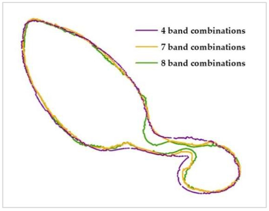
Figure 14.
Detection results of Yinli Shoal based on different band combinations of WorldView-3 image.
4.3. Application of the Proposed Method
The detection method proposed in this study is expected to provide the coral shoals’ information rapidly once optical satellite images are available and cloud cover and tropical cyclones are satisfactory. However, tropical cyclones can cause significant changes to coral shoals in a very short period of time [64,65], so the imaging time of the satellite images for detecting coral shoals should be avoided before and after the occurrence of tropical cyclones. For this reason, it is vital to understand the knowledge of the tropical cyclones’ features in the study area and forecast the tropical cyclones phenomena in advance. Related studies indicate that a study area belongs to the region where an earlier study found the changes of tropical cyclone features during the recent period, in a manner that similar changes can be expected to occur in the future [66]. Moreover, the time series of the tropical cyclones count obeys the classical random walk (white noise) or, in other words, they do not exhibit long-term memory [67]. Therefore, the long-term forecasting of tropical cyclones is difficult and the short-term advance forecasting is commonly used. The combination of sequential and cluster analysis with the percolation procedure allows for the detection of a tropical cyclone up to 1-3 days in advance of its start, which has been applied in a set of devastating tropical cyclones such as Franklin, Harvey, Irma, and Katia [68,69]. The further integration of the detection results of coral shoals with water depth and other information can effectively ensure the safe navigation of ships.
5. Conclusions
An optical remote sensing detection method based on DBN is proposed to rapidly and accurately detect coral shoals in satellite imagery. The median filter is used to filter the DBN classification results, and the appropriate filtering window is selected according to the spatial resolution of optical images. The outstanding performance of this detection method is demonstrated by validating and comparing the Yinli Shoal’s results. Furthermore, this method reveals successful applicability to the other coral shoals in the Xisha Islands. Future studies should explore its applicability to a wider range of coral shoals worldwide. This detection method is expected to rapidly provide the coral shoals’ information once optical satellite images are available and cloud cover and tropical cyclones are satisfactory. Therefore, it is necessary to forecast tropical cyclones in advance to confirm that they will not occur during remote sensing imaging. The further integration of the detection results of coral shoals with water depth and other information can effectively ensure the safe navigation of ships.
Author Contributions
Conceptualization, X.L. and J.Z.; Methodology, X.L. and Y.M.; Data collection and curation, X.L.; Writing—original draft, X.L.; Writing—review and editing, Y.M.; Project administration, Y.M. and J.Z.; Funding acquisition, J.Z. All authors have read and agreed to the published version of the manuscript.
Funding
This research was funded by the National Key R&D Program of China (2022YFC3105100).
Institutional Review Board Statement
Not applicable.
Informed Consent Statement
Not applicable.
Data Availability Statement
GF-1 satellite data are free-of-charge and are available from the China Center for Resources Satellite Data and Application: https://www.cresda.com/zgzywxyyzx/index.html (accessed on 31 July 2017). QuickBird, Worldview-2/3, and SPOT-6 images presented in this study were purchased by the authors and their team with the support of relevant projects, and are available on request from the corresponding author (J.Z.).
Acknowledgments
The authors would like to thank China’s High-Resolution Earth Observation System Major Project for its support, as well as the China Center for Resources Satellite Data and Application for providing GF-1 PMS and WFV data.
Conflicts of Interest
The authors declare no conflicts of interest.
References
- Zhao, H.T.; Wang, L.R.; Song, C.J. Geomorphological model of coral reefs in the South China Sea. Acta Oceanol. Sin. 2014, 36, 112–120. [Google Scholar]
- Bellwood, D.R.; Hughes, T.P. Regional-scale assembly rules and biodiversity of coral reefs. Science 2001, 292, 1532–1535. [Google Scholar] [CrossRef] [PubMed]
- Zhao, M.X.; Yu, K.F.; Zhang, Q.M. Review on coral reefs biodiversity and ecological function. Acta Ecol. Sin. 2006, 26, 186–194. [Google Scholar]
- David, W.S.; Olof, L. The health and future of coral reef systems. Ocean Coast. Manag. 2000, 43, 657–688. [Google Scholar]
- Zhao, H.T.; Wang, L.R. Review on the study of formation mechanism of coral reefs. Trop. Geog. 2016, 36, 1–9. [Google Scholar]
- Smith, S.V. Coral-reef area and contributions of reefs to processes and resources of the World’s Oceans. Nature 1978, 273, 225–226. [Google Scholar] [CrossRef]
- Azmath, J. The status of the coral reefs and the management approaches: The case of the Maldives. Ocean Coast. Manag. 2013, 82, 104–118. [Google Scholar]
- Huang, R.Y.; Yu, K.F.; Wang, Y.H.; Liu, J.L.; Zhang, H.Y. Progress of the study on coral reef remote sensing. J. Remote Sens. 2019, 23, 1091–1112. [Google Scholar] [CrossRef]
- Xu, J.P.; Zhao, D.Z. Review of coral reef ecosystem remote sensing. Acta Ecol. Sin. 2014, 34, 19–25. [Google Scholar] [CrossRef]
- Hedley, J.D.; Roelfsema, C.M.; Chollett, I.; Harborne, A.R.; Heron, S.F.; Weeks, S.; Skirving, W.J.; Strong, A.E.; Eakin, C.M.; Christensen, T.R.L.; et al. Remote sensing of coral reefs for monitoring and management: A review. Remote Sens. 2016, 8, 118. [Google Scholar] [CrossRef]
- Roelfsema, C.; Phinn, S.; Jupiter, S.; Comley, J.; Albert, S. Mapping coral reefs at reef to reef-system scales, 10s–1000s km2, using object-based image analysis. Int. J. Remote Sens. 2013, 34, 6367–6388. [Google Scholar] [CrossRef]
- Awak, D.S.; Gaol, J.L.; Subhan, B.; Madduppa, H.H.; Arafat, D. Coral reef ecosystem monitoring using remote sensing data: Case study in Owi Island, Biak, Papua. Procedia Environ. Sci. 2016, 33, 600–606. [Google Scholar] [CrossRef]
- Wulder, M.A.; Loveland, T.R.; Roy, D.P.; Crawford, C.J.; Masek, J.G.; Woodcock, C.E.; Allen, R.G.; Anderson, M.C.; Belward, A.S.; Cohen, W.B.; et al. Current status of Landsat program, science, and applications. Remote Sens. Environ. 2019, 225, 127–147. [Google Scholar] [CrossRef]
- Capolsini, P.; Andréfouët, S.; Rion, C.; Payri, C. Landsat ETM+, SPOT HRV, IKONOS, ASTER, and airborne MASTER data for coral reef habitat mapping in South Pacific islands. Can. J. Remote Sens. 2003, 29, 187–200. [Google Scholar] [CrossRef]
- Andréfouët, S.; Kramer, P.; Torres-Pulliza, D.; Joyce, K.E.; Hochberg, E.J.; Garza-Pérez, R.; Mumby, P.J.; Riegl, B.; Yamano, H.; White, W.H.; et al. Multi-site evaluation of IKONOS data for classification of tropical coral reef environments. Remote Sens. Environ. 2003, 88, 128–143. [Google Scholar] [CrossRef]
- Hedley, J.D.; Roelfsema, C.; Brando, V.; Giardino, C.; Kutser, T.; Phinn, S.; Mumby, P.J.; Barrilero, O.; Laporte, J.; Koetz, B. Coral reef applications of Sentinel-2: Coverage, characteristics, bathymetry and benthic mapping with comparison to Landsat-8. Remote Sens. Environ. 2018, 216, 598–614. [Google Scholar] [CrossRef]
- Asner, G.P.; Martin, R.E.; Mascaro, J. Coral reef atoll assessment in the south china sea using planet dove satellites. Remote Sens. Ecol. Conserv. 2017, 3, 57–65. [Google Scholar] [CrossRef]
- Lyons, M.B.; Roelfsema, C.M.; Kennedy, E.V.; Kovacs, E.M.; Borrego-Acevedo, R.; Markey, K.; Roe, M.; Yuwono, D.M.; Harris, D.L.; Phinn, S.R. Mapping the world’s coral reefs using a global multiscale earth observation framework. Remote Sens. Ecol. Conserv. 2020, 6, 557–568. [Google Scholar]
- Duvat, V.K.E.; Pillet, V. Shoreline changes in reef islands of the Central Pacific: Takapoto Atoll, Northern Tuamotu, French Polynesia. Geomorphology 2017, 282, 96–118. [Google Scholar] [CrossRef]
- Ford, M. Shoreline changes interpreted from multi-temporal aerial photographs and high resolution satellite images: Wotje Atoll, Marshall Islands. Remote Sens. Environ. 2013, 135, 130–140. [Google Scholar] [CrossRef]
- Li, X.M.; Ma, Y.; Zhang, J.; Lyu, X.X. Spatial and temporal dynamics of typical islands in the Xishan Islands using high-resolution satellite images. Mar. Sci. Bull. 2020, 39, 717–729. [Google Scholar]
- Aslam, M.; Kench, P.S. Reef island dynamics and mechanisms of change in Huvadhoo Atoll, Republic of Maldives, Indian Ocean. Anthropocene 2017, 18, 57–68. [Google Scholar] [CrossRef]
- Duvat, V.K.E.; Salvat, B.; Salmon, C. Drivers of shoreline change in atoll reef islands of the Tuamotu Archipelago, French Polynesia. Global Planet. Chang. 2017, 158, 134–154. [Google Scholar] [CrossRef]
- Duvat, V.K.E. Human-driven atoll island expansion in the Maldives. Anthropocene 2020, 32, 100265. [Google Scholar] [CrossRef]
- Kench, P.S.; Parnell, K.E.; Brander, R.W. Monsoonally influenced circulation around coral reef islands and seasonal dynamics of reef island shorelines. Mar. Geol. 2009, 266, 91–108. [Google Scholar] [CrossRef]
- Liu, J.L.; Huang, R.Y.; Yu, K.F.; Zou, B. How lime-sand islands in the South China Sea have responded to global warming over the last 30 years: Evidence from satellite remote sensing images. Geomorphology 2020, 371, 107423. [Google Scholar] [CrossRef]
- Webb, A.P.; Kench, P.S. The dynamic response of reef islands to sea-level rise: Evidence from multi-decadal analysis of island change in the Central Pacific. Global Planet. Chang. 2010, 72, 234–246. [Google Scholar] [CrossRef]
- Zhu, H.T.; Jiang, X.W.; Meng, X.L.; Feng, Q.; Cui, S.X. A quantitative approach to monitoring new sand cay migration in Nansha Islands. Acta Oceanol. Sin. 2016, 35, 102–107. [Google Scholar] [CrossRef]
- Zhou, S.N.; Shi, Q.; Guo, H.Y.; Yang, H.Q.; Yan, H.Q. Evolution of Coral Shingle Cays in the Nansha Islands during 2009–2017. Trop. Geog. 2020, 40, 694–708. [Google Scholar]
- Li, X.M.; Ma, Y.; Zhang, J.; Lyu, X.X. Assessing the stability of coral reef sandbanks in the Xisha Islands using high-resolution satellite images. Mar. Environ. Sci. 2022, 41, 48–58. [Google Scholar]
- Phinn, S.R.; Roelfsema, C.M.; Mumby, P.J. Multi-scale, object-based image analysis for mapping geomorphic and ecological zones on coral reefs. Int. J. Remote Sens. 2012, 33, 3768–3797. [Google Scholar] [CrossRef]
- Leon, J.; Woodroffe, C.D. Improving the synoptic mapping of coral reef geomorphology using object-based image analysis. Int. J. Geogr. Inf. Sci. 2011, 25, 949–969. [Google Scholar] [CrossRef]
- Xu, J.P.; Zhao, J.H.; Li, F.; Wang, L.; Song, D.R.; Wen, S.Y.; Wang, F.; Gao, N. Object-based image analysis for mapping geomorphic zones of coral reefs in the Xisha Islands, China. Acta Oceanol. Sin. 2016, 35, 19–27. [Google Scholar] [CrossRef]
- Dong, Y.Z.; Liu, Y.X.; Hu, C.M.; Xu, B.H. Coral reef geomorphology of the Spratly Islands: A simple method based on time-series of Landsat-8 multi-band inundation maps. ISPRSJ. Photogramm. Remote Sens. 2019, 157, 137–154. [Google Scholar] [CrossRef]
- Dong, J.; Ren, G.B.; Hu, Y.B.; Pang, J.Z.; Ma, Y. Construction and classification of coral reef geomorphic unit system based on high-resolution remote sensing: Using 8-band Worldview-2 image as an example. J. Trop. Oceanogr. 2020, 39, 116–129. [Google Scholar]
- Benfield, S.L.; Guzman, H.M.; Mair, J.M.; Young, J.A.T. Mapping the distribution of coral reefs and associated sublittoral habitats in Pacific Panama: A comparison of optical satellite sensors and classification methodologies. Int. J. Remote Sens. 2007, 28, 5047–5070. [Google Scholar] [CrossRef]
- Saul, S.; Purkis, S. Semi-automated object-based classification of coral reef habitat using discrete choice models. Remote Sens. 2015, 7, 15894–15916. [Google Scholar] [CrossRef]
- Li, J.W.; Schill, S.R.; Knapp, D.E.; Asner, G.P. Object-based mapping of coral reef habitats using planet Dove satellites. Remote Sens. 2019, 11, 1445. [Google Scholar] [CrossRef]
- Zhou, M.X.; Liu, Y.X.; Li, M.C.; Sun, C.; Zou, W. Geomorphologic information extraction for multi-objective coral islands from remotely sensed imagery: A case study for Yongle Atoll, South China Sea. Geogr. Res. 2015, 34, 677–690. [Google Scholar]
- Sun, Q.P.; Ma, Y.; Sun, W.F.; Zhang, J.Y. Research on reef remote sensing detection based on GVF snake model: Taken Yinlitan for example. In Proceedings of the 2016 IEEE International Geoscience and Remote Sensing Symposium, Beijing, China, 10–15 July 2016; pp. 717–720. [Google Scholar]
- Hinton, G.E.; Salakhutdinov, R.R. Reducing the dimensionality of data with neural networks. Science 2006, 313, 504–507. [Google Scholar] [CrossRef]
- Schmidhuber, J. Deep learning in neural networks: An overview. Neural Netw. 2015, 61, 85–117. [Google Scholar]
- LeCun, Y.; Bengio, Y.; Hinton, G. Deep learning. Nature 2015, 521, 436–444. [Google Scholar] [CrossRef]
- Liu, J.W.; Liu, Y.; Luo, X.L. Research and development on deep learning. Appl. Res. Comput. 2014, 31, 1921–1930. [Google Scholar]
- Ball, J.E.; Anderson, D.T.; Chan, C.S. A comprehensive survey of deep learning in remote sensing: Theories, tools, and challenges for the community. J. Appl. Remote Sens. 2017, 11, 042629. [Google Scholar] [CrossRef]
- Hinton, G.E.; Osindero, S.; Teh, Y. A fast learning algorithm for deep belief nets. Neural Comput. 2006, 18, 1527–1554. [Google Scholar] [CrossRef] [PubMed]
- Mnih, V.; Hinton, G.E. Learning to detect roads in high resolution aerial images. In Computer Vision—ECCV 2010, Proceedings of the 2010 European Conference Computer Vision, Piscataway, NJ, USA, 5–11 September 2010; Springer: Berlin/Heidelberg, Germany, 2010; pp. 210–223. [Google Scholar]
- Lv, Q.; Dou, Y.; Niu, X.; Xu, J.; Xia, F. Remote sensing image classification based on DBN model. J. Comput. Res. Dev. 2014, 51, 1911–1918. [Google Scholar]
- Lv, Q.; Dou, Y.; Niu, X.; Xu, J.; Xu, J.; Xia, F. Urban land use and land cover classification using remotely sensed SAR data through deep belief networks. J. Sens. 2015, 2015, 1–10. [Google Scholar] [CrossRef]
- Xu, L.K.; Liu, X.D.; Xiang, X.C. Recognition and classification for remote sensing image based on depth belief network. Geol. Sci. Technol. Inf. 2017, 36, 244–249. [Google Scholar]
- Navy Hydrographic Survey Bureau of the People’s Liberation Army of China. China Navigation Guidelines: South China Sea Area; China Navigation Book Press: Tianjin, China, 2022. [Google Scholar]
- Ying, M.; Zhang, W.; Yu, H.; Lu, X.; Feng, J.; Fan, Y.; Zhu, Y.; Chen, D. An overview of the China Meteorological Administration tropical cyclone database. J. Atmos. Ocean. Technol. 2014, 31, 287–301. [Google Scholar] [CrossRef]
- Lu, X.Q.; Yu, H.; Ying, M.; Zhao, B.K.; Zhang, S.; Lin, L.M.; Bai, L.N.; Wan, R.J. Western North Pacific tropical cyclone database created by the China Meteorological Administration. Adv. Atmos. Sci. 2021, 38, 690–699. [Google Scholar] [CrossRef]
- Wu, B.Y. Practical Algorithm for Atmospheric Radiation Transfer; China Meteorological Press: Beijing, China, 1998; pp. 6–10. [Google Scholar]
- Hinton, G.E. Deep belief networks. Scholarpedia 2009, 4, 5947. [Google Scholar] [CrossRef]
- Fischer, A. Training restricted Boltzmann machines. Kunstl. Intell. 2015, 29, 441–444. [Google Scholar] [CrossRef]
- Kass, M.; Witkin, A.; Terzopoulos, D. Snakes: Active contour models. Int. J. Comput. Vis. 1988, 1, 321–331. [Google Scholar] [CrossRef]
- Chen, L.C.; Niu, Y.M.; Pan, L.H.; Zhang, X.Q. Research advances on Snake model. Appl. Res. Comput. 2014, 31, 1931–1936. [Google Scholar]
- Xu, C.Y.; Prince, J.L. Gradient Vector Flow: A new external force for Snake. In Proceedings of the IEEE Computer Society Conference on Computer Vision and Pattern Recognition, San Juan, PR, USA, 17–19 June 1997; pp. 66–71. [Google Scholar]
- Lu, D.; Weng, Q. A survey of image classification methods and techniques for improving classification performance. Int. J. Remote Sens. 2007, 28, 823–870. [Google Scholar] [CrossRef]
- Bandyopadhyay, S.; Sharma, S.; Bahuguna, A. Artificial neural network based coral cover classifiers using Indian Remote Sensing (IRS LISS-III) sensor data: A case study in gulf of Kachcch, India. Int. J. Geoinf. 2009, 5, 55–63. [Google Scholar]
- Gapper, J.J.; EI-Askary, H.; Linstead, E.; Piechota, T. Coral reef change detection in remote Pacific Islands using support vector machine classifiers. Remote Sens. 2019, 11, 1525. [Google Scholar] [CrossRef]
- Chegoonian, A.M.; Mokhtarzade, M.; Zoej, M.J.V. A comprehensive evaluation of classification algorithms for coral reef habitat mapping: Challenges related to quantity, quality, and impurity of training samples. Int. J. Remote Sens. 2017, 38, 4224–4243. [Google Scholar] [CrossRef]
- Ford, M.R.; Kench, P.S. Spatiotemporal variability of typhoon impacts and relaxation intervals on Jaluit Atoll, Marshall Islands. Geology 2016, 44, 159–162. [Google Scholar] [CrossRef]
- Duvat, V.K.E.; Volto, N.; Salmon, C. Impacts of category 5 tropical cyclone Fantala (April 2016) on Farquhar Atoll, Seychelles Islands, Indian Ocean. Geomorphology 2017, 298, 41–62. [Google Scholar] [CrossRef]
- Varotsos, C.A.; Efstathiou, M.N.; Cracknell, A.P. Sharp rise in hurricane and cyclone count during the last century. Theor. Appl. Climatol. 2015, 119, 629–638. [Google Scholar] [CrossRef]
- Varotsos, C.A.; Efstathiou, M.N. Is there any long-term memory effect in the tropical cyclones? Theor. Appl. Climatol. 2013, 114, 643–650. [Google Scholar] [CrossRef]
- Krapivin, V.F.; Soldatov, V.Y.; Varotsos, C.A.; Cracknell, A.P. An adaptive information technology for the operative diagnostics of the tropical cyclones; solar–terrestrial coupling mechanisms. J. Atmos. Sol.-Terr. Phys. 2012, 89, 83–89. [Google Scholar] [CrossRef]
- Varotsos, C.A.; Krapivin, V.F.; Soldatov, V.Y. Monitoring and forecasting of tropical cyclones: A new information-modeling tool to reduce the risk. Int. J. Disaster Risk Reduct. 2019, 36, 101088. [Google Scholar] [CrossRef]


Disclaimer/Publisher’s Note: The statements, opinions and data contained in all publications are solely those of the individual author(s) and contributor(s) and not of MDPI and/or the editor(s). MDPI and/or the editor(s) disclaim responsibility for any injury to people or property resulting from any ideas, methods, instructions or products referred to in the content. |
© 2024 by the authors. Licensee MDPI, Basel, Switzerland. This article is an open access article distributed under the terms and conditions of the Creative Commons Attribution (CC BY) license (https://creativecommons.org/licenses/by/4.0/).