Experimental Investigation of Ice Loads on Structures during Quasi-Static Compression Tests

Abstract

In polar ship hull structural designs, methods based on regulations are considered the most authoritative; however, they tend to be conservative and often exhibit a notable degree of redundancy. This study aims to evaluate the applicability of the empirical formula for ice load assessments by conducting a series of quasi-static indentation tests on scaled hull plates under laboratory-made ice blocks of different scales. The obtained data include ice loads, structural responses, and characteristics of ice pressure distribution. A detailed comparison of various formulas is provided, along with an examination of their differences and errors in comparison to experimental results. The objective of this paper is to offer technical support for ice load forecasting and assessment.

1. Introduction

The exploration and utilization of polar regions have attracted significant global attention, particularly due to the abundant fossil energy resources found in the Arctic region. Polar vessels inevitably encounter the impact of ice loads during navigation in icy regions, which involves a complex interaction process. It is widely acknowledged that the magnitude of ice loads depends on various factors such as the mechanical characteristics of the ice, the interaction mode between ice and structures, the geometric shape and dimensions of structures, the thickness and speed of ice blocks, and the failure mode of ice. Regarding the interaction mode between structures and ice, ice loads primarily result from processes involving compression, bending, and fracturing damage to ice floes, level ice, or icebergs. Notably, the compressive load imposed by ice is particularly significant and requires focused attention when assessing ship structure stability and safety.

The investigation of ice loads on bridges, piles, and structures has received considerable attention from scholars. Empirically based methods for assessing ice loads offer the advantages of convenience and efficiency. A widely accepted classical empirical formula was proposed by Korzhavin [1], who conducted extensive research on the characteristics of river ice loads based on measurements of dynamic and static pressures in Siberia. Similarly, Croasdale, Michel, Frederking, and other researchers employed similar on-site or experimental measurement methods [2,3,4], with variations in the types of ice studied, such as lake ice and freshwater ice. Currently, several classification societies and standard organizations, including Bureau Veritas (BV) [5] and the International Organization for Standardization (ISO) [6] recommend using empirically based methods for assessing ice loads. As methodologies continue to expand and improve, there is an active pursuit of organizational initiatives [7]. Masterson and Tibbo [8] conducted a comparative analysis of the different assumptions used in calculating ice loads based on measured data from Timco and Croasdale [9]. Kellner [10] provided a comprehensive review of current code-based methods for predicting ice loads. Barker [11] conducted experimental investigations on the structural ice loads during the interaction between sea ice and cone structures. To this end, they employed seven model structures and analyzed the influence of ice speed, thickness, structural form, and stiffness on the ice loads acting on the models. Based on observing the process of ice breaking and the accumulation of broken ice, Li [12] measured the load and the size of broken ice and analyzed the influence of ship speed and ice thickness on the formation and accumulation of broken ice. Zong [13] used polypropylene wax to simulate floating ice and analyzed the characteristics of sea ice. With advancements in simulation technology, finite element calculations are increasingly being used for predicting and assessing ice loads, which serve as effective means for code-based verification [14,15,16]. Truong [17] proposed an ice pressure estimation method based on the numerical simulation stress response data influence coefficient method (ICM) and compared the estimated local ice pressure with the simulation results. The results show that the results are in good agreement under single dynamic loading cases, and the results are slightly deviated under dynamic loading combination cases. Based on the extended finite element method, Xu [18] verified the ice load obtained by the numerical simulation of the collision between ice and a rigid ship with the field test data. The results show that the numerical method is in good agreement with the ice load data obtained by the test. Zheng [19] used the ship–ice–water SPH method to analyze the predicted ice-breaking resistance under different conditions. The results show that the ice resistance is positively correlated with the bending strength and ice thickness, and the latter is the most important factor affecting the ice resistance. In summary, achieving a cohesive theoretical framework remains challenging when anticipating ice loads. Further research efforts require a stronger foundation of experimental data that aligns with the primary objective of this work.

The present study provides an introduction to the prevailing methodologies for static ice load prediction based on codes and empirical formulas. Additionally, quasi-static loading tests were conducted to investigate the interaction between local ship structures and the ice. This study compares the magnitude and variations of ice loads obtained from experimental measurements with theoretical calculations, thereby evaluating the efficacy and applicability of empirical methods for estimating ice loads. The purpose of this paper is to obtain a fast prediction method for ice load on flat structures under static ice extrusion. The relevant research results have positive significance for polar structural safety assessment and ice load prediction.

2. Quasi-Static Compression Experiments on Ice–Structure Interaction

2.1. Uniaxial Compression and Three-Point Bending Tests of Ice Specimens

The ice samples used in this study are polycrystalline ice made in the laboratory. This involved a process of freezing size-controlled crushed ice and degassed water. The requisite protocol for preparing these samples included an initial freezing phase in a controlled environment at −20 °C for 48 h, followed by a subsequent storage period exceeding two days in a defrost freezer before their utilization in the experiments. Compression and three-point bending tests (Support Span 60 mm) were conducted to acquire fundamental material parameters. The design of specimen dimensions adhered to the guidelines recommended by the International Association for Hydro-Environment Engineering and Research (IAHR) [20]. The compression specimens were sized at 70 mm × 70 mm × 175 mm, while the bending specimens measured 75 mm × 75 mm × 700 mm. The setup for these tests is illustrated in Figure 1.

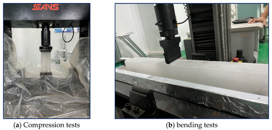
Figure 1. Compression and bending test setup for ice specimens.

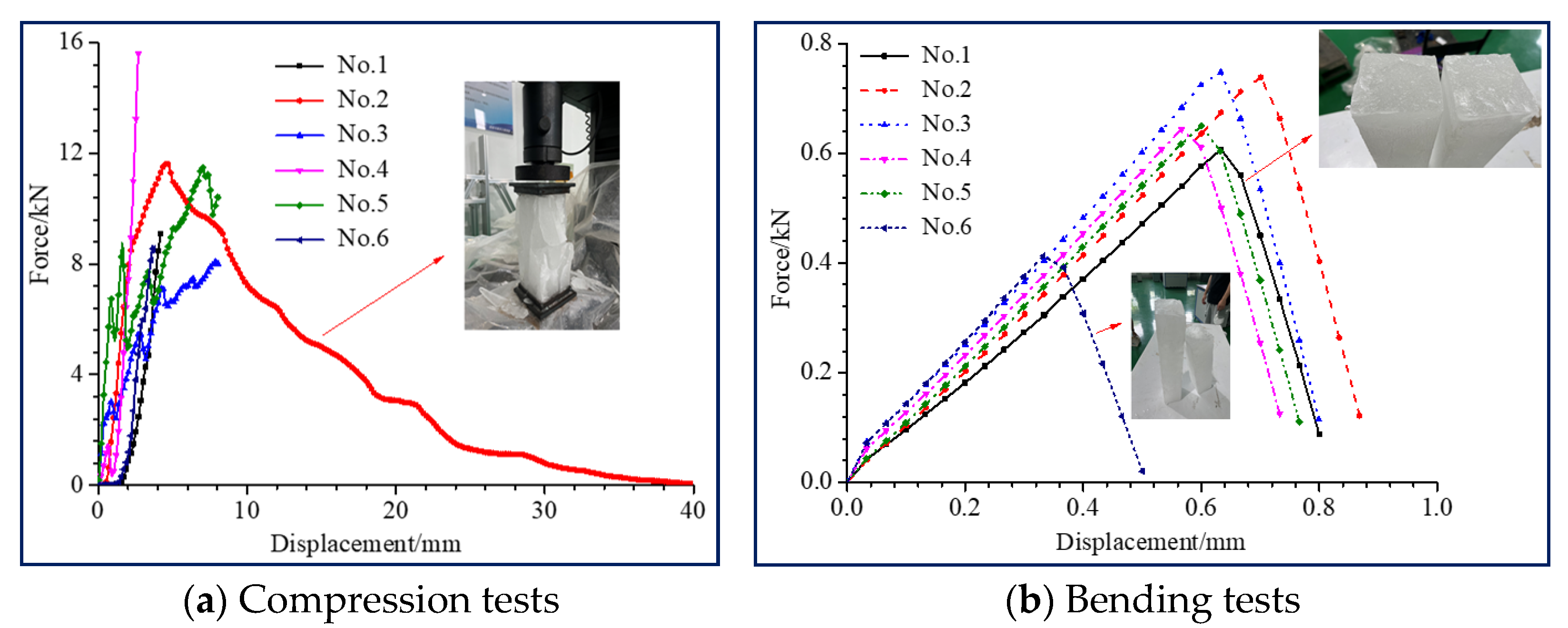
During the tests, data on load and actuator displacement were recorded, and the mechanical parameters were computed accordingly, as illustrated in Figure 2. The calculated bending and compression strengths of the ice samples are presented in Table 1 and Table 2. The mechanical properties assessment, as well as the subsequent quasi-static extrusion test of the structure–ice interface, were conducted under controlled laboratory conditions, with an ambient temperature of 25 °C, and the installation preparation time was 3 min. The loading speed was set at 1 mm/s.

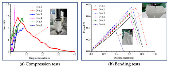
Figure 2. Load–displacement curve of the ice sample compression and bending tests.

Table 1. Calculated compressive strength of ice samples.

Test Number	Ambient Temperature (°C)	Compressive Strength (MPa)	Mean Compressive Strength (MPa)
No.1	25	1.86	2.20
No.2	25	2.37
No.3	25	1.65
No.4	25	3.19
No.5	25	2.35
No.6	25	1.77

Table 2. Calculated bending strength of ice samples.

Test Number	Ambient Temperature (°C)	Bending Strength (MPa)	Mean Bending Strength (MPa)
No.1	25	1.59	1.66
No.2	25	1.93
No.3	25	1.96
No.4	25	1.69
No.5	25	1.71
No.6	25	1.02

The compression and bending strengths of the ice samples obtained by freezing crushed ice were found to be within the range of typical strength values for natural existing ice (typically, 0.5 MPa~5 MPa for uniaxial compressive strength and 1 MPa~2 MPa for bending strength) [21]. Moreover, it is evident that the experimental results demonstrate good stability. As shown in Figure 2, the results of six compression tests of ice show similar brittle failure. The load–displacement curves show a multi-peak shape. The six bending tests of the ice body are also brittle failures, and the fracture position is slightly different. The load peaks and curves of compression and bending tests show certain differences because the ice samples prepared in the laboratory cannot be standardized. It should be noted that the variability observed in bending test No. 6 can be attributed to inherent defects in the test specimen itself.

2.2. The Experimental Setup and Its Implementation

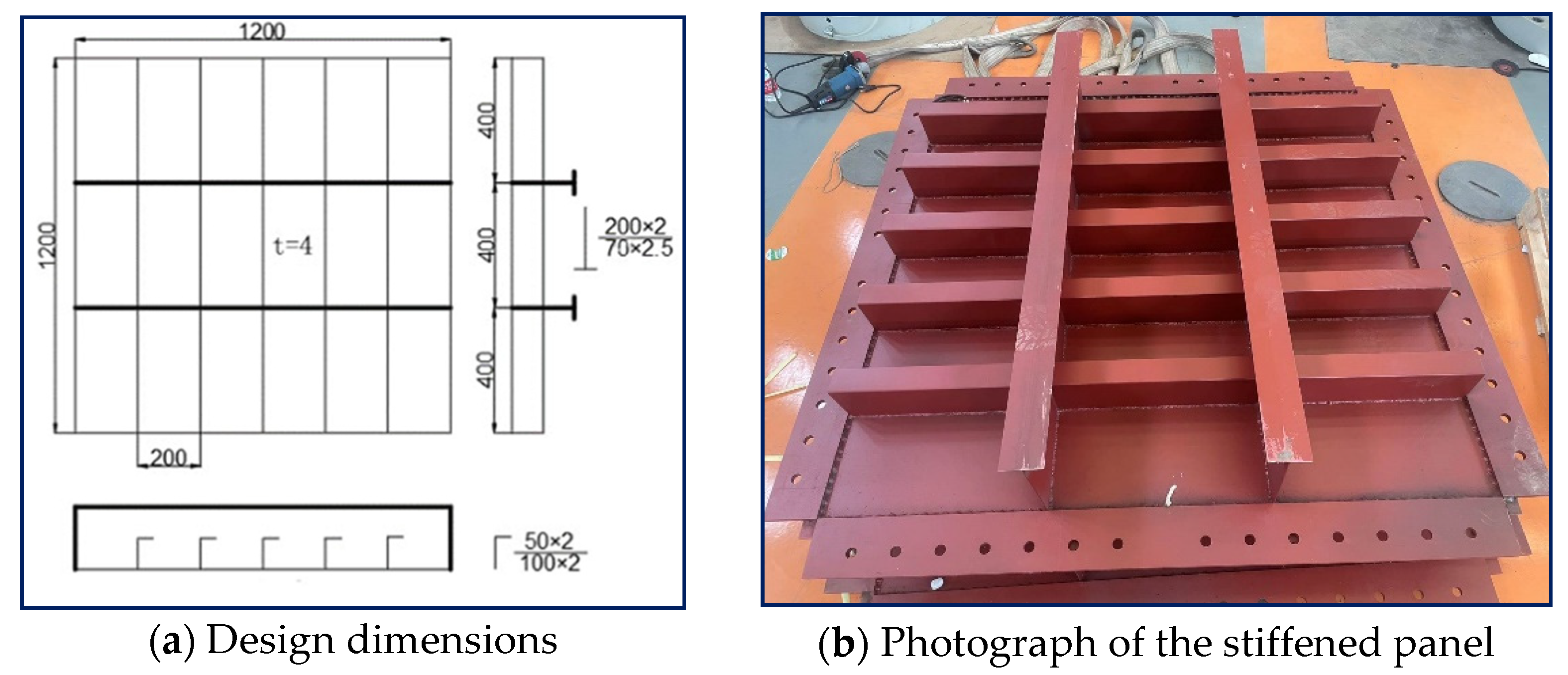
The primary objective of the model test is to investigate the underlying mechanism during the ice-breaking process and evaluate methodologies for calculating ice loads. The stiffened panel, as illustrated in Figure 3, utilized in the experiments was scaled down from a specific ship’s partial structure, with its design dimensions depicted in Figure 3a. Comprising panels, reinforcing members, and girders are all constructed from mild steel (Q235), and the stiffened panel consists of three distinct types of components.

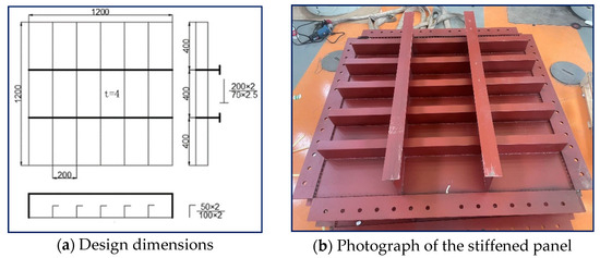
Figure 3. The stiffened panel was used in the experiment.

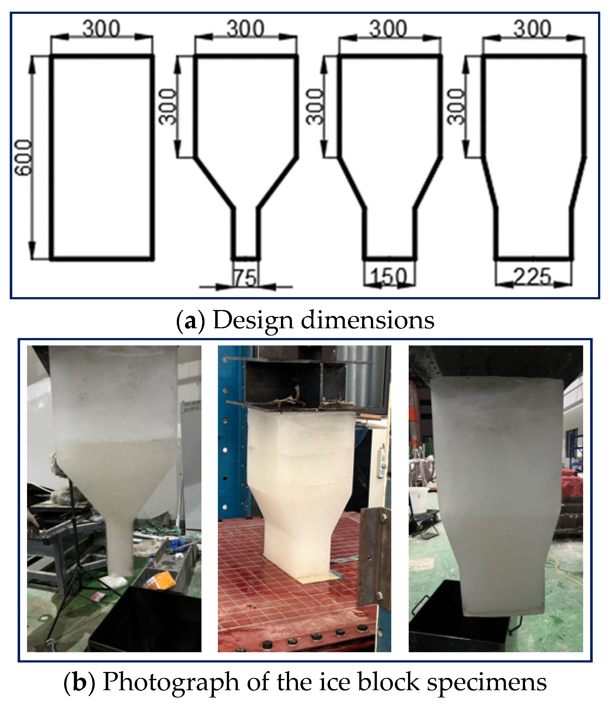
In the experimental setup, the ice block specimens are classified into three distinct types based on their respective contact areas: specifically, 300 mm × 75 mm, 300 mm × 150 mm, and 300 mm × 225 mm. All of the ice block specimens have a height of 600 mm, a top-end width of 300 mm, and a thickness of 300 mm, as depicted in Figure 4.

Figure 4. The ice block specimens were used in the experiment.

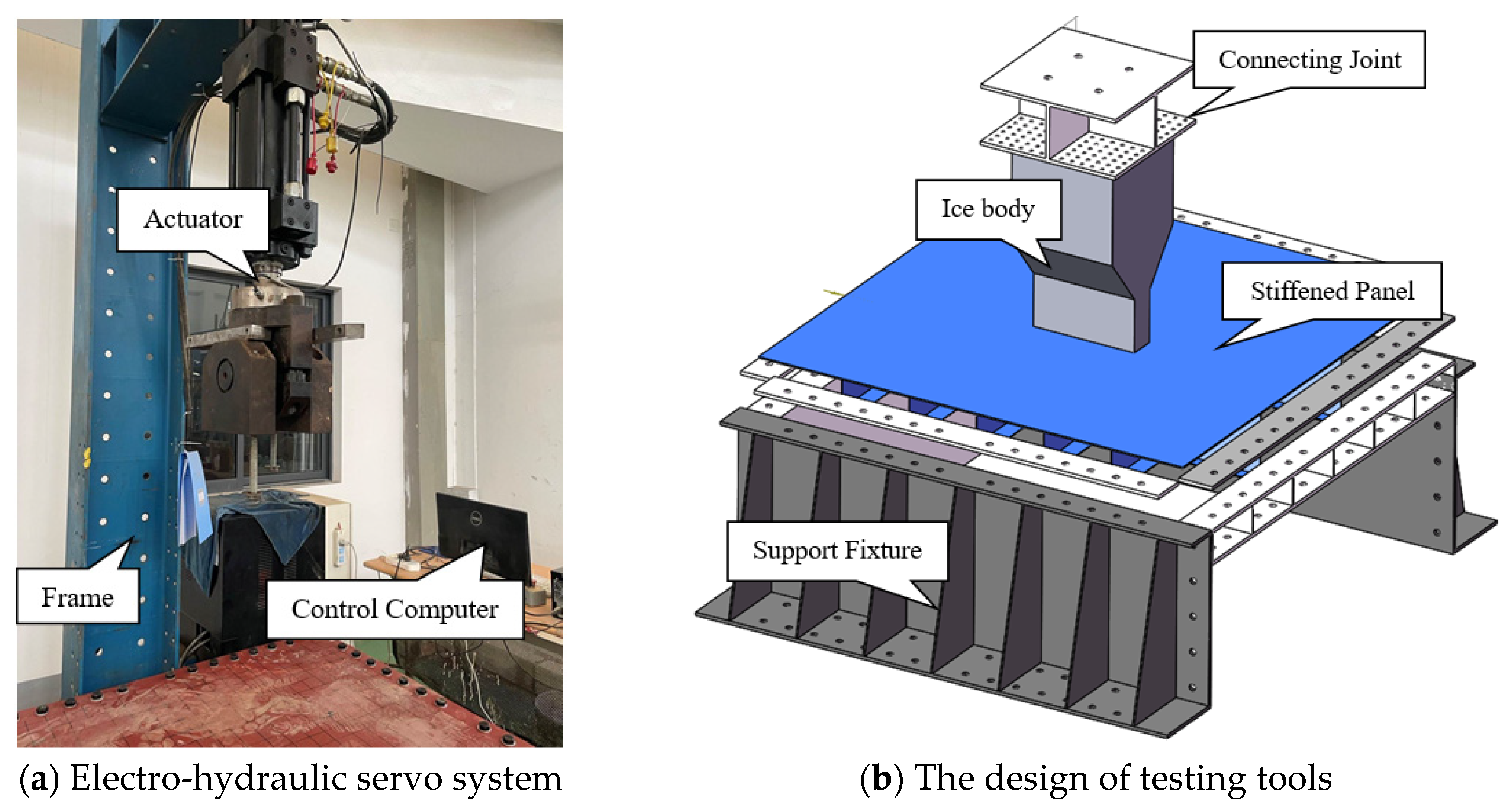
The quasi-static compression tests were performed using a 10-ton electro-hydraulic servo system, as illustrated in Figure 5a. A set of meticulously designed fixtures was developed and utilized in the experiments, as depicted in Figure 5b. The connecting joint acts as an intermediary between the ice block and the actuator. The upper section of the joint is securely fastened to the actuator using bolts, while the lower section is integrated with the ice block through freezing with hemp ropes. The stiffened panel is bolted to the support fixtures, which are specifically designed to provide ample rigidity, ensuring that there is no deformation within the frame’s boundaries. It should be noted that during the experiment, the longer side of the ice block’s lower part was aligned parallel to the direction of the stiffeners, while its shorter side was perpendicular to them. The actuator’s speed was set at 1 mm/s, and load and displacement data were systematically recorded throughout each process. Three replicated experiments have been conducted for each type of ice block.

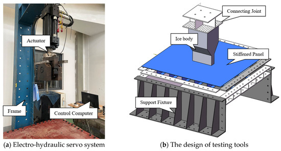
Figure 5. Test loading system.

2.3. Experimental Results

2.3.1. Analysis of Ice Failure Mode

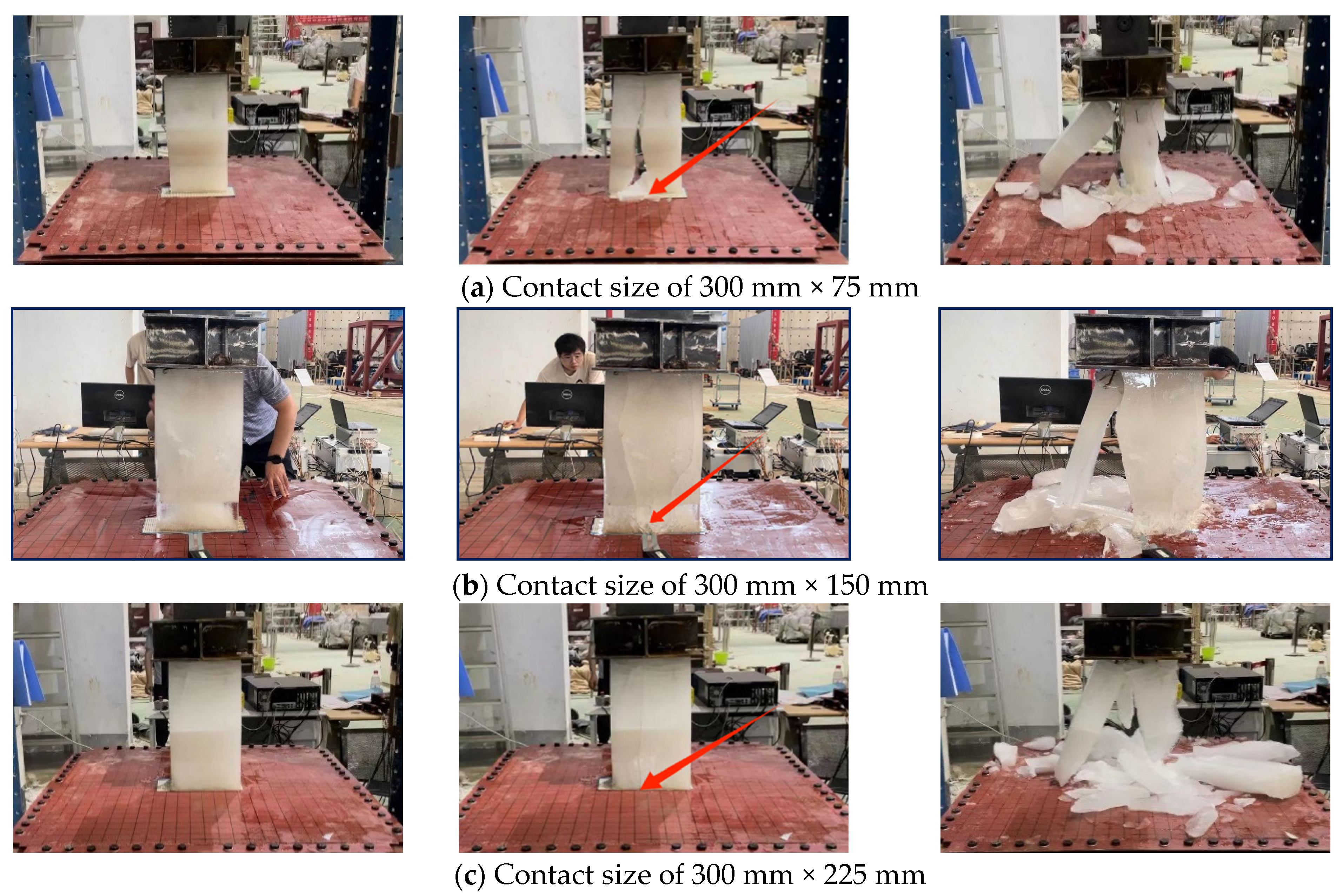
The quasi-static compressive experiment in Figure 6 presents an image sequence depicting the interaction process between the ice block and stiffened panel with varying contact sizes. It is evident that regardless of the contact size, significant cracking consistently occurs at the middle stiffener of the panel (indicated by red arrows) due to the enhanced strength at these locations, rendering the ice block incapable of sustaining applied shear loads. When subjected to contact sizes of 300 mm × 75 mm and 300 mm × 150 mm, spalling occurs as a result of major cracking damage in the ice; however, a substantial load-bearing capacity is maintained by the remaining ice block. In contrast, when using a contact surface size of 300 mm × 225 mm, direct crushing of the ice takes place, leading to destruction characterized by pronounced shattering.

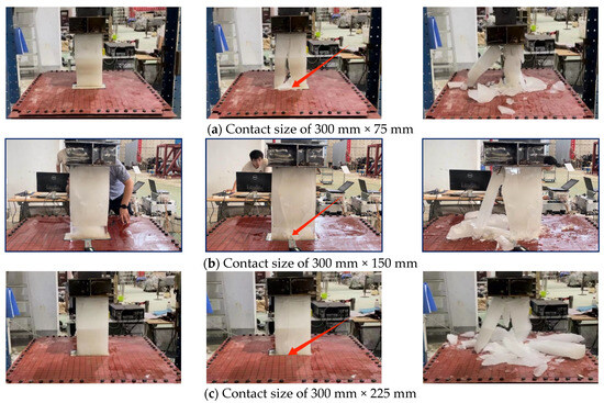
Figure 6. Ice destruction process with different contact sizes.

2.3.2. Structural Deformation

No significant or easily observable plastic deformation was observed in the stiffened panel in all test cases. Only when the contact area is relatively large does a minor indentation deformation occur, as depicted in Figure 7. The maximum deformation measured was approximately 6 mm. Due to the presence of a middle stiffener, the deformation is evenly distributed on both sides of it and remains within a relatively narrow range. Based on photographic evidence from the experimental procedure, it can be inferred that the panel’s deformation primarily stems from residual ice blockage following major cracking. This observation suggests that even after fracture, the ice block retains considerable load-bearing capacity.

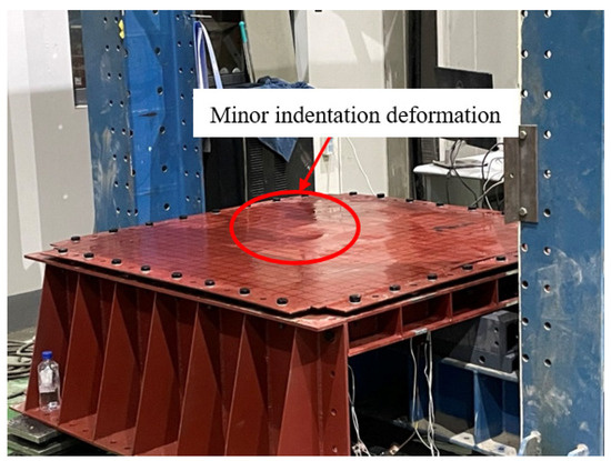
Figure 7. Deformation of the stiffened panel (contact area: 300 mm × 225 mm).

2.3.3. Load–Displacement Data during the Test Process

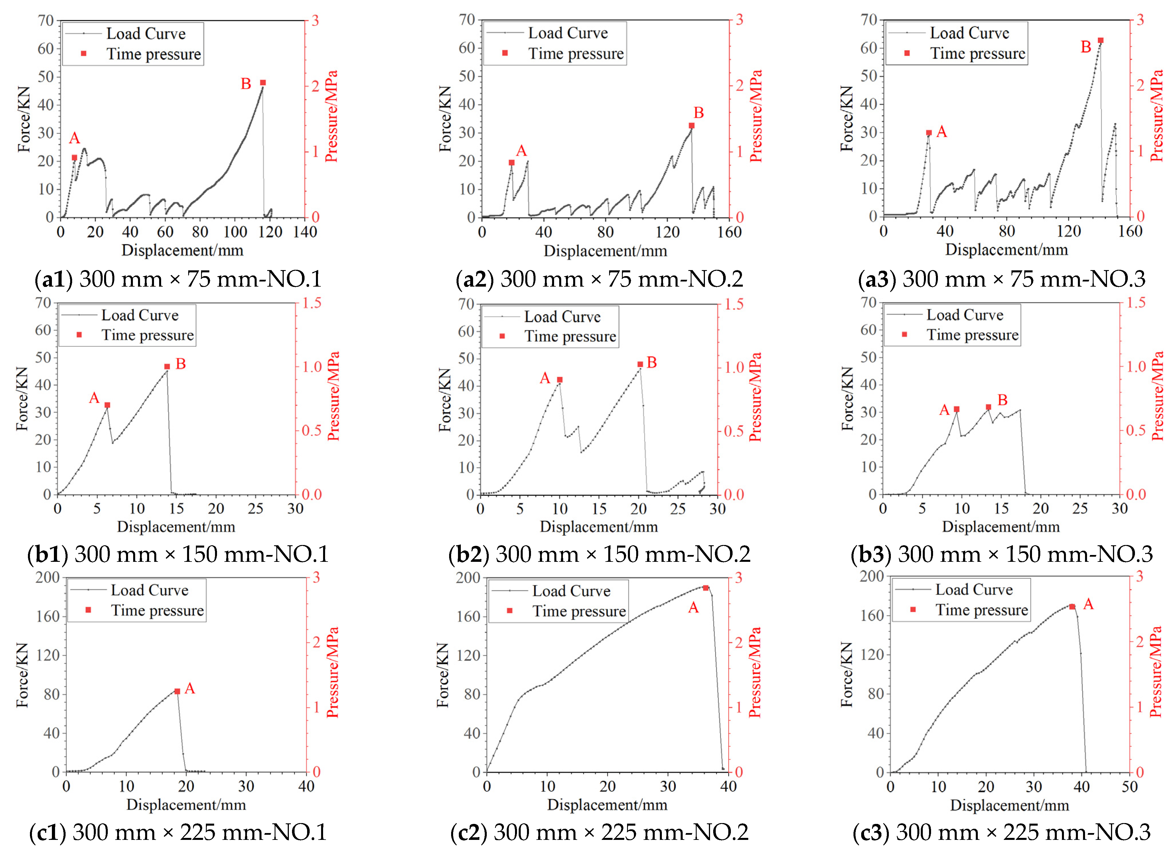
Figure 8 presents the load–displacement curves under different contact sizes. It can be observed that during the compression process, the load curves exhibit characteristics of slow loading and rapid unloading in all cases. The load–displacement curve changes effectively reflect the ice block’s failure process. When the contact size is 300 mm × 75 mm, the load curve exhibits typical non-linear characteristics with multiple peaks. The maximum peak load of the first peak load can reach 29.04 KN, and the minimum is 18.83 KN. The failure process of the ice in the three repeated tests reflects the random destructiveness of the ice, and similar load variation characteristics are observed. The first peak values are 20.72 KN, 18.83 KN, and 29.04 KN, respectively. In addition, it can be clearly seen that the maximum peak load in the test is significantly greater than the first peak (45.79 KN, 29.63 KN, and 61.61 KN), indicating that the bearing capacity of residual ice is indeed great. When the contact size is 300 mm × 150 mm, the peak number is significantly reduced, the displacement value is significantly reduced, and the uniformity is stable at about 20 mm, and the repeated test load characteristics also reflect similarity. The maximum peak loads recorded were 45.20 KN, 46.46 KN, and 30.17 KN, respectively. When the contact size is 300 mm × 225 mm, the load–displacement curve exhibits only a single peak, with the peak values being 84.54 KN, 189.47 KN, and 171.6 KN, respectively. This result stems from the fact that the contact area between the stiffened plates and the ice bodies of this series is the greatest compared to the other two series. Furthermore, following the vertical cracking failure of the ice body at the rib, no ice body suffered a fracture or detachment during the subsequent loading process. The ice body continued to withstand loading until it surpassed its maximal bearing capacity, at which point it fractured and ceased contact with the plate. Under this condition, the ice body shows brittle failure. The reason for the smaller load in the first test is still due to the sliding of the smaller ice blocks after cracking, as shown in Figure 8(c3).

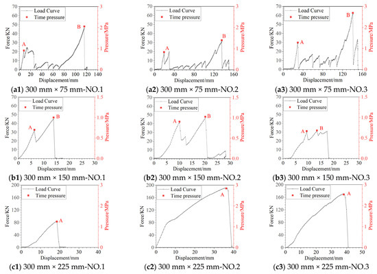
Figure 8. Load–displacement curves under various contact sizes.

Point A and point B represent the pressure values corresponding to the first peak load and the maximum peak load moment, respectively. These values are calculated by the moment load and the initial contact area, as shown in Figure 8. It is worth noting that when the contact area is 300 mm × 225 mm and the load curve only shows one peak, the first peak load value is equal to the maximum load value. Further, Table 3 records the pressure data under different working conditions in detail. Through the analysis of these data, we can observe that the overall trend of the pressure value increases with an increase in the contact area. However, there is an interesting phenomenon that when the contact area is 300 mm × 150 mm, the corresponding pressure value is lower than that when the contact area is 300 mm × 75 mm. After in-depth analysis, we found that this is mainly because during the test, the first peak load and the maximum load measured when the contact area is 300 mm × 150 mm are almost the same as those when the contact area is 300 mm × 75 mm. However, because the contact area of the former is twice that of the latter, this abnormal pressure value occurs.

Table 3. Load and pressure values under different sizes.

Case Number	First Peak Load (KN)	First Peak Pressure (MKN)	Maximum Load (KN)	Maximum Load Pressure (MKN)
300 mm × 75 mm-NO.1	20.72	0.92	45.79	2.06
300 mm × 75 mm-NO.2	18.83	0.84	29.63	1.40
300 mm × 75 mm-NO.3	29.04	1.20	29.04	2.70
300 mm × 150 mm-NO.1	31.68	0.70	45.20	1.00
300 mm × 150 mm-NO.2	40.97	0.91	46.46	1.03
300 mm × 150 mm-NO.3	30.17	0.67	30.94	0.69
300 mm × 225 mm-NO.1	84.54	1.25	84.54	-
300 mm × 225 mm-NO.2	190.45	2.85	190.45	-
300 mm × 225 mm-NO.3	171.60	2.54	171.60	-

The first peak load along with the maximum load values under different cases are summarized in Table 3. It is observed that the maximum load values demonstrate a nonlinear positive correlation with the contact area. Additionally, it should be noted that, for some of the working conditions, the initial peak load is identical to the maximum peak load.

3. Static Ice Load Calculation Method

Currently, ice load calculation standards have been implemented in countries such as the United States and Canada, with numerous scholars developing their empirical formulas based on experimental findings. It is important to note that, for the safety of Arctic navigation, a significant portion of ice load research primarily focuses on sea ice phenomena like icebergs and level ice. However, countries with extensive inland regions and cold climates, such as the former Soviet Union, also attach great importance to studying ice loads in inland rivers. Nevertheless, the fundamental principle of calculating ice loads remains straightforward, that is, as follows:

$$F={\sigma }_{\max }A$$

(1)

Herein, $F$, ${\sigma }_{\max }$, and $A$ respective variables represent the calculated ice force, the compressive strength of the ice, and the area of mutual contact. This formula holds for static conditions with a flat contact surface and the absence of friction. However, considering practical application scenarios, it becomes imperative to take into account factors such as the projected area component on the vertical cross-section of the contact surface and parameters related to slippage. Consequently, a revision is necessary to develop an empirical calculation method. Currently, there are various empirical formulas available for calculating static ice force, which can be broadly classified into categories based on linear functions and those founded on exponential functions.

3.1. The Method of Predicting Static Ice Loads Based on Linear Formulas

The magnitude of ice loads is influenced by multiple factors, and the empirical formulas are typically characterized by the quantitative representation of various parameters. In their initial stages, these formulas were commonly linear, with both single and multiple coefficients to facilitate computational simplicity, as demonstrated in Equation (2).

$$F=\alpha Dh{\sigma }_c$$

(2)

In the formula, $D$ represents the projected width of the structure’s ice-facing surface, $h$ denotes the thickness of the ice, ${\sigma }_c$ is indicative of the uniaxial compressive strength of the ice, and $\alpha$ accounts for comprehensive correction factors that consider modifications to the actual stress state caused by variables such as ice velocity, contact conditions, and local compression. These formulas incorporate experimental findings and theoretical approaches, possessing explicit physical significance while maintaining dimensional consistency and broad applicability. Based on linear formulas, static ice loads primarily rely on both the uniaxial compressive strength of the ice and the contact area between it and the structure. Table 4 provides a summary of similar formulas [22].

Table 4. The calculation formula for static ice load is based on the linear formula.

Name	Expression	Meaning of the Parameters	Background
Korzhavin	$F=I{\left(V/V_0\right)}^{-1/3}mKDH{\sigma }_c$	$I$: local compression coefficient; $v$: relative velocity; $v_0$: reference velocity; $m$: structural shape coefficient; $K$: contact condition coefficient; $H$: ice thickness.	Based on a large number of experimental data and theoretical analysis of Siberian rivers.
Afanasev (1971)	$F=ImDh{\sigma }_c$$,I\left\{\begin{array}{l}{(1+5\times H/D)}^{1/2}(1<D/H\le 6)\\ 2.5(D/H=6)\\ 4.17-1.67D/H(0.1<D/H\le 1)\\ 4.0(D/H=1)\end{array}\right.$	$I$: local compression coefficient; $m$: structural shape coefficient.	Based on Korzhavin, further research is carried out, and the calculation method under different D/H ratios is obtained.
Lu	For vertical piers: $F=aCDH{\sigma }_{\mathrm{c}}$ For inclined piers, horizontal force: $F_H=a_w{H}^2\tan \beta$ Vertical force: $F_V=a_{\mathrm{w}}^{\sigma }{H}^2$	$a$: regional coefficient; $C$: comprehensive correction coefficient; ${\sigma }_w$: ice’s flexural strength; $\beta$: the angle of inclination of the ice-breaking edge of the bridge pier.	This paper is based on a large number of experiments on the ice pressure on the No.3 pier of the Songhua River Bridge caused by the ice flow in the Hal Glacier section of the Songhua River in China.
Former Soviet Union’s standards	$F=ImDh{\sigma }_c$	$I$: local compression coefficient.	Based on the Arctic coastline scene of the former Soviet Union, the ice pressure acting on the vertical pier is analyzed.
Russian Ice Load Regulations	$F={\phi }_{i}DH{\sigma }_c$	${\phi }_i$: structural ice-facing surface shape coefficient; $H$: ice thickness.	The ice surface of the bridge pier is vertical, and the ice load on the bridge pier is applied.
American API2A Formula	$F=CDH{\sigma }_c$	$C$: coefficient dependent on the structural shape, ice velocity, and other factors.	For the flowing ice force acting on a single column, the larger the ratio of pile diameter to ice thickness, the smaller the coefficient ‘c’.
American APIRP2N Formula	$F=ImKDh{\sigma }_c$	$I$: local compression coefficient; $K$: contact coefficient.	Based on the ice flow force on a single column in the Cook Bay of Alaska, USA.
Canadian CAS Formula (1974)	$F=Dh{P}_c$	$P_c$: effective ice pressure.	Based on the unique ice environment and cold temperate climate in Canada, the force of flowing ice on buildings is proposed.
Canadian Standards for Bridge Piers	$F=C_{n}DH{\sigma }_c$	$C_n$: inclination coefficient of bridge pier fore-edges.	Based on different inclination angles of the leading edge of the pier, there are different inclination coefficients.
Canadian Lighthouse Formula (1975)	$F=mDh{\sigma }_c$	$m$: comprehensive correction coefficient.	Ensure that the Canadian offshore lighthouse structure can withstand the ice load that may be suffered under extreme conditions.
Chinese Offshore Platform Standards	$F=m{K}_1{K}_{2}Dh{\sigma }_c$	$K_1$: local compression coefficient; $K_2$: contact coefficient; ${\sigma }_c$: ice’s compressive strength.	Under the action of wind and current, the ice load of a large area of the ice sheet on the vertically isolated pile.

3.2. Exponential Formula-Based Predictive Method for Static Ice Loads

The expression method for static ice loads, established by Schwarz through regression analysis of experimental data from model experiments, is based on an exponential formula and can be articulated as follows:

$$F=\beta D^{0.5}{H}^{\gamma }{\sigma }_c$$

(3)

In the formula, $\beta$ represents a correction coefficient that is typically a constant value under particular environmental circumstances.

This type of formula represents an advancement in the existing methods for calculating ice loads, which were initially developed based on linear formulas and subsequently refined by incorporating various exponential terms derived from extensive experimental data. It is specifically tailored to suit particular environmental conditions, with a relatively limited scope of application and involving parameters that lack dimensional consistency. However, it offers highly targeted results with enhanced precision. Such formulas are presented in Table 5 [22]. This category of formulas combines and simplifies the influence of different factors from the first category of formulas on the calculation of ice forces, thereby providing unique practical value for real-world applications.

Table 5. Calculation formula of static ice load based on the exponential formula.

Name	Expression	Notes	Background
Schwarz Formula	$F=3.75D^{0.5}{H}^{1.1}{\sigma }_c$	$F$: unit in KN; $D$: unit in $\mathrm{cm}$; ${\sigma }_c$: unit in $\mathrm{KN}/{\mathrm{cm}}^2$.	A large number of experimental and theoretical studies have been conducted in the Baltic Sea, North Sea, and North Atlantic, and a multi-coefficient formula is proposed.
Hamayaka Formula	$F=C{D}^{0.5}H{\sigma }_c$	$C$: correction coefficient. For circular cross-sections, it takes 5.0; for rectangular cross-sections, it takes 6.8.	Based on the ice situation in the Beibu Gulf of Japan.

4. Comparison of Ice Load Magnitudes from Experiments and Empirical Formulas

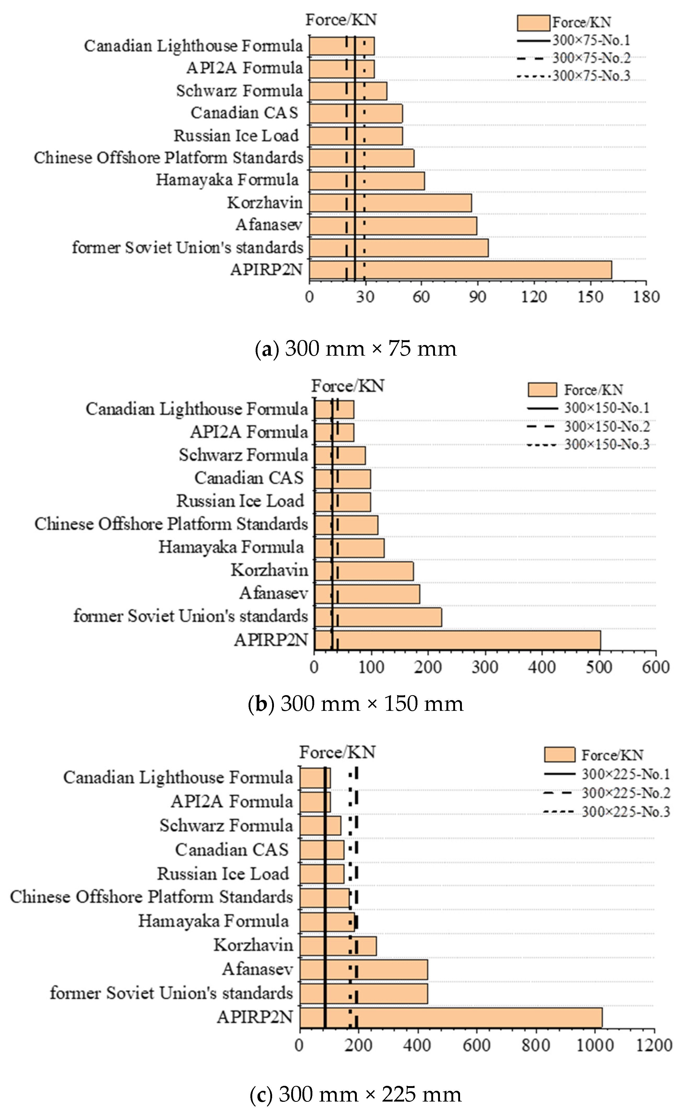
The present study meticulously compiles empirical methodologies for estimating ice loads on marine piles and bridge piers. Given the analogous loading patterns observed in side shell structures with significant stiffness, the extrapolation of these empirical formulas to such constructions is considered justifiable. By disregarding the progressive disintegration of the ice block, we adopt the initial peak value on the load–displacement curve as the reference experimental load, facilitating a comparative analysis with outcomes derived from various empirical formulas, as depicted in Figure 9. It is evident that results obtained from the same empirical formula positively correlate with the contact area. Due to the conservative parameters and assumptions employed in standards and empirical formulas, the resultant load values generated in practice are comparatively higher. Notably, when the aspect ratio of the contact area is smaller, discrepancies in load estimations predicted by these methods become more pronounced. Additionally, it can be observed that the calculation results from the APIRP2N formula consistently overestimate. This can primarily be attributed to contact coefficients being derived from ice conditions in Cook Inlet, Alaska, USA, where parameter values are significantly higher than those used in other standards.

Figure 9. Comparison of results from various empirical formulas with actual measurement data.

5. Discussion

5.1. Comparative Analysis of Different Empirical Formulas

5.1.1. Identifying the Factors for Determining Correction Coefficient

The correction coefficient, as mentioned previously, is an empirical value obtained by fitting a large set of experimental data. It may be a composite correction factor or consist of multiple sub-factors to collectively account for the influence of various factors. The determination of this coefficient should consider the following considerations:

(1) Contact state between ice and structure

In both categories of formulas (Equations (2) and (3)), the compressive strength ${\sigma }_C$ is determined through uniaxial compression tests. However, it should be noted that these tests do not consider the three-dimensional stress state of ice, which significantly enhances its strength under confining pressure. This distinction is crucial in understanding different scenarios, such as ship collisions with ice flies or icebergs and the compression of river ice against bridge piers. Therefore, when dealing with substantial ice thicknesses, it becomes necessary to further calibrate the correction coefficient to account for the enhanced strength beyond what is determined by uniaxial compression.

(2) Ice–structure contact conditions

In ice force calculation formulas, ‘Dh’ ($Dh$ in Equation (2) and $D^i{H}^j$ in Equation (3)) represents the projected contact area between ice and the structure. However, due to the brittle nature of ice, the spalling of ice fragments results in numerous irregular notches, thereby reducing the effective contact area. The faster the compression rate of ice, the more pronounced this effect becomes. Moreover, it is unlikely for the entire ice mass to attain its ultimate strength and fail uniformly across the actual contact area, leading to disparities between theoretical and practical contact areas. It should be noted that strain rate and interaction velocity are closely intertwined; however, in real-world scenarios, sea ice velocity near structural entities exhibits significant variability. Consequently, adjusting parameters α and β may not yield tangible engineering benefits in such contexts. Therefore, only the Korzhavin formula incorporates both strain rate and uniaxial compressive strength.

5.1.2. Ice Load Magnitude and Contact Surface Shape Characteristics

In the second category of formulas, the formulas are obtained by applying an exponential transformation to the length and width dimensions of the contact surface in the first category. Consequently, the influencing factors to be considered are similar, among which the most critical is the shape and angle of the contact surface.

(1) Structural shape coefficient

The shape factor ‘m’ represents the influence of the structural shape on ice forces and is generally determined based on the shape of the structure’s ice-facing surface. Typically, a value of 1 is commonly assigned for flat contact surfaces, while cylindrical (or semi-circular) surfaces are often given a value of 0.9. For angular shapes, which are defined by the vertex angle ‘$2\alpha$’, the corresponding value can be obtained from Table 6 [23].

Table 6. Shape coefficient values for different angles.

2α	45°	60°	75°	90°	120°	180°
m	0.6	0.65	0.69	0.73	0.81	1.0

In certain empirical formulas (see Table 1), the impact of the inclination coefficient on ice loads needs to be considered. Table 7 presents the ratios of numerical force to horizontal force under varying inclination coefficients (angles) [24]. It is noteworthy that at inclination angles exceeding a certain threshold (commonly 30°), the mode of ice failure may transition from compressive to bending failure. Consequently, in such scenarios, the calculation of ice pressure should employ the bending strength of the ice, necessitating corresponding modifications to the computational formulas.

Table 7. The ratio of vertical to horizontal forces under various inclination coefficients.

Inclination Angle		Inclination Coefficient Cn	The Ratio of Vertical to Horizontal Forces FV/FH
α	β
0	90	1.00	0
15	75	0.75	0.11
20	70	0.75	0.20
25	65	0.75	0.29
30	60	0.75	0.39
35	55	0.50	0.50
40	50	0.50	0.61
45	45	0.50	0.74

5.2. Modification of the Korzhavin Formula Based on Experimental Outcomes

The Korzhavin formula, as a classic method for static ice load prediction, encompasses a comprehensive range of parameters. Additionally, based on the comparative results presented earlier, the Korzhavin formula demonstrates superior applicability and accuracy relative to other empirical formulas. The loading conditions of this experiment comply with the requirements of the Korzhavin formula, thereby justifying its use for calculating ice loads. Therefore, attention must be focused on the selection of the local compression coefficient ‘I’. The literature indicates that when the width of the ice floe exceeds 15 times the pile diameter, ‘I’ should be set at 2.5. However, this method of determination is evidently inapplicable in the context of this study. To enhance the alignment of the Korzhavin formula with the specific research object, it is imperative to amend the localized compression coefficient incorporated in the formula that is not consistent with the authentic research conditions. Therefore, we propose a fresh interpretation of the compression coefficient based on the test environment and results. Such a modification will ensure greater accuracy in our investigations. A compression coefficient deduced from experimental results is presented in Table 8.

Table 8. Comparison of results from improved Korzhavin formula and experiments.

Case Number	First Peak Load (KN)	Local Compression Coefficient Value	Average Compression Coefficient	COV (Coefficient of Variation)	Empirical Formula-Derived Ice Loads (KN)	Relative Error (%)
300 mm × 75 mm-NO.1	20.72	0.71	0.70	0.7/2.5 = 0.28	24.15	1.79
300 mm × 75 mm-NO.2	18.83	0.54				28.25
300 mm × 75 mm-NO.3	29.04	0.84				16.84
300 mm × 150 mm-NO.1	31.68	0.42	0.49	0.49/2.5 = 0.196	33.90	7.01
300 mm × 150 mm-NO.2	40.97	0.46				17.26
300 mm × 150 mm-NO.3	30.17	0.59				12.36
300 mm × 225 mm-NO.1	84.54	0.61	1.07	1.07/2.5 = 0.428	111.23	31.57
300 mm × 225 mm-NO.2	190.45	1.37				41.59
300 mm × 225 mm-NO.3	171.60	1.24				35.18

It is observable that the localized compression coefficients derived from experimental results are consistently lower than 2.5. If a discrepancy of 30% is considered acceptable, then, with the exception of certain cases, the overall error margin between the ice load calculated using empirical formulas and that obtained from experiments generally falls within an acceptable range, with the minimum error being 1.79%. This observation substantiates the rationality of the employed empirical formula.

6. Conclusions

This study focuses on the prediction of quasi-static ice loads, employing a comprehensive review of empirical formula-based forecasting methods and validation through quasi-static compression tests of ice–structure interaction. An assessment of the accuracy and applicability of various empirical calculation methods was conducted. The conclusions are as follows:

(1)

Various standards and empirical formulas exist for static ice load prediction, which can be classified into two main types based on their formulation: linear and exponential. In practical applications, the results obtained from different empirical formulas often exhibit significant variation due to variations in engineering contexts, ice conditions, etc.

(2)

Quasi-static compression tests of ice–structure interaction were conducted. The stiffened panel did not undergo any noticeable or easily observable plastic deformation. In all the tests studied in this paper, the ice block consistently exhibits significant cracking at the middle stiffener of the panel, and the maximum load values demonstrate a nonlinear positive correlation with the contact area.

(3)

A comprehensive discourse on the determination of various parameters was undertaken, encompassing aspects such as the correction coefficient, characteristics of the contact surface shape, and the structural shape coefficient. The Korzhavin formula is shown to exhibit enhanced applicability and precision in comparison to other empirical formulas. Therefore, a compression coefficient deduced from experimental results is presented, which also substantiates the empirical formula’s rationality and efficacy.

Using the model test method, the ice load size and load change can be directly obtained and further compared with the calculated values of the empirical formula. However, due to certain error limitations of the test technology, it is impossible to accurately simulate and restore the real ice-breaking scene. In addition, the factors that affect the accuracy of the empirical formula will be further studied, and the test technology will be continuously improved in the future.

References

- Korzhavin, K.N. Action of Ice on Engineering Structures; Defense Technical Information Center: Fort Belvoir, VA, USA, 1962.
- Croasdale, K.R.; Morgenstern, N.R.; Nuttall, J.B. Indentation Tests to Investigate Ice Pressures on Vertical Piers. J. Glaciol. 1977, 19, 301–312. [Google Scholar] [CrossRef]
- Michel, B.; Toussaint, N. Mechanisms and Theory of Indentation of Ice Plates. J. Glaciol. 1977, 19, 285–300. [Google Scholar] [CrossRef]
- Frederking, R.; Timco, G.; Reid, S. Sea Ice Floe Impact Experiments; National Research Council of Canada: Quebec, QC, Canada, 1999. [Google Scholar] [CrossRef]
- Veritas, B. NI565 Ice Characteristics and Ice/Structure Interactions. Guidance Note NI, 2010. Available online: https://marine-offshore.bureauveritas.com/ni565-ice-characteristics-and-icestructure-interactions (accessed on 28 March 2024).
- ISO19906:2019(E); Petroleum and Natural Gas Industries—Arctic Offshore Structures. ISO: Geneva, Switzerland, 2019.
- Masterson, D.M.; Kouzmitchev, K.; deWaal, J. Russian SNiP 2.06.04-82 and Western Global Ice Pressures–A Comparison. In Proceedings of the 17th International Conference on Port and Ocean Engineering under Arctic Conditions, Trondheim, Norway, 16–19 June 2003. [Google Scholar]
- Masterson, D.M.; Susan Tibbo, J. Comparison of Ice Load Calculations Using ISO 19906, CSA, API and SNiP. In Proceedings of the 21st International Conference on Port and Ocean Engineering under Arctic Conditions (POAC’11), Montréal, QC, Canada, 10–14 July 2011; Volume 2. [Google Scholar]
- Timco, G.; Croasdale, K. How Well Can We Predict Ice Loads? IAHR 2006, 1, 167–174. [Google Scholar]
- Kellner, L.; Herrnring, H.; Ring, M. Review of Ice Load Standards and Comparison with Measurements. In Proceedings of the International Conference on Offshore Mechanics and Arctic Engineering–OMAE, American Society of Mechanical Engineers, Trondheim, Norway, 25–30 June 2017; Volume 57762, p. V008T07A028. [Google Scholar]
- Gravesen, H.; Sørensen, S.L.; Vølund, P.; Barker, A.; Timco, G. Ice Loading on Danish Wind Turbines: Part 2. Analyses of Dynamic Model Test Results. Cold Reg. Sci. Technol. 2005, 41, 25–47. [Google Scholar] [CrossRef]
- Zhou, L.; Riska, K.; von Bock und Polach, R.; Moan, T.; Su, B. Experiments on Level Ice Loading on an Icebreaking Tanker with Different Ice Drift Angles. Cold Reg. Sci. Technol. 2013, 85, 79–93. [Google Scholar] [CrossRef]
- Zong, Z.; Yang, B.Y.; Sun, Z.; Zhang, G.Y. Experimental Study of Ship Resistance in Artificial Ice Floes. Cold Reg. Sci. Technol. 2020, 176, 103102. [Google Scholar] [CrossRef]
- Su, B. Numerical Predictions of Global and Local Ice Loads on Ships. Ph.D. Thesis, Norwegian University of Science and Technology, Trondheim, Norway, 2011. [Google Scholar]
- Liu, Z.; Amdahl, J.; Løset, S. Numerical Simulation of Collisions between Ships and Icebergs. In Proceedings of the International Conference on Port and Ocean Engineering under Arctic Conditions, POAC, Lulea, Sweden, 9–12 June 2009; Volume 1. [Google Scholar]
- Yu, T.; Liu, K.; Wang, G.; Liu, J.; Wang, Z. A Tri-Axial Ice Model for Simulating Ice-Stiffened Panel Impact: Experiments and Numerical Modeling. Mar. Struct. 2023, 88, 103358. [Google Scholar] [CrossRef]
- Truong, D.D.; Jang, B.-S. Estimation of Ice Loads on Offshore Structures Using Simulations of Level Ice-Structure Collisions with an Influence Coefficient Method. Appl. Ocean Res. 2022, 125, 103235. [Google Scholar] [CrossRef]
- Xu, Y.; Wu, J.; Li, P.; Kujala, P.; Hu, Z.; Chen, G. Investigation of the Fracture Mechanism of Level Ice with Extended Finite Element Method. Ocean Eng. 2022, 260, 112048. [Google Scholar] [CrossRef]
- Zheng, X.; Tian, Z.; Xie, Z.; Zhang, N. Numerical Study of the Ice Breaking Resistance of the Icebreaker in the Yellow River Through Smoothed-Particle Hydrodynamics. J. Mar. Sci. Appl. 2022, 21, 1–14. [Google Scholar] [CrossRef]
- Schwarz, J.; Frederking, R.; Gavrillo, V.; Petrov, I.G.; Hirayama, K.I.; Mellor, M.; Tryde, P.; Vaudrey, K.D. Standardized Testing Methods for Measuring Mechanical Properties of Ice. Cold Reg. Sci. Technol. 1981, 4, 245–253. [Google Scholar] [CrossRef]
- Timco, G.W.; Weeks, W.F. A Review of the Engineering Properties of Sea Ice. Cold Reg. Sci. Technol. 2010, 60, 107–129. [Google Scholar] [CrossRef]
- Wang, G.; Zhang, D.; Xu, N.; Wang, S.; Yu, D.; Yue, Q. The Research of Extreme Ice Load for Flexible Vertical Structures in Sub-Arctic Environment. Ekoloji 2018, 27, 2033. [Google Scholar]
- Rødtang, E.; Alfredsen, K.; Høyland, K.; Lia, L. Review of River Ice Force Calculation Methods. Cold Reg. Sci. Technol. 2023, 209, 103809. [Google Scholar] [CrossRef]
- Neill, C.R. Dynamic ice forces on piers and piles. An assessment of design guidelines in the light of recent research. Can. J. Civil. Eng. 1976, 3, 305–341. [Google Scholar] [CrossRef]
Disclaimer/Publisher’s Note: The statements, opinions and data contained in all publications are solely those of the individual author(s) and contributor(s) and not of MDPI and/or the editor(s). MDPI and/or the editor(s) disclaim responsibility for any injury to people or property resulting from any ideas, methods, instructions or products referred to in the content. |
© 2024 by the authors. Licensee MDPI, Basel, Switzerland. This article is an open access article distributed under the terms and conditions of the Creative Commons Attribution (CC BY) license (https://creativecommons.org/licenses/by/4.0/).