Dual-Mode Square Root Cubature Kalman Filter for Miniaturized Underwater Profiler Dead Reckoning

Abstract

Miniaturized underwater profilers have the advantages of small size, low cost, and flexible deployment, which play together an important role in the persistent monitoring of a designated ocean area. Based on the demand for ocean observation, the system design, dynamic modeling, and dead reckoning algorithm of a miniaturized underwater profiler are carried out. The process of the persistent monitoring of designated area with a miniaturized underwater profiler is analyzed, and the overall structure of the miniaturized underwater profiler was designed. Additionally, the kinematic and dynamic model of the miniaturized underwater profiler is given based on the inertial and body coordinate systems. Then, according to the state equation and the observation equation of the miniaturized underwater profiler, a dual-mode square root cubature Kalman filter (DSRCKF) algorithm, combining standard SRCKF and adaptive SRCKF, is proposed for the dead reckoning of the miniaturized underwater profiler. Finally, a comprehensive comparison of EKF, UKF, CKF, SRCKF, and DSRCKF and the associated simulations and experiments are conducted to verify the performance of the underwater dead reckoning algorithm for the miniaturized underwater profiler. The results show that the DSRCKF algorithm has a certain role in the dead reckoning of the miniaturized underwater profiler, particularly in the z direction and attitude. In future, a real underwater dead reckoning test using miniaturized underwater profiler will be carried out.

1. Introduction

Ocean designated area persistent monitoring technology can obtain small range and long-term ocean data, providing data support for the comprehensive and reliable analysis of ocean-related phenomena. It is thus important in terms of its application in military exploration and in the observation of major ocean emergencies. As a result, countries attach great importance to the research and development of ocean observation technology [1]. As underwater designated area monitoring platforms, miniaturized underwater profilers have the advantages of low noise, low cost, small size, convenient transportation, and flexible deployment. Therefore, this study focuses on the relevant content of a miniaturized underwater profiler in ocean designated area persistent monitoring technology.

Currently, the common underwater mobile platforms that can perform designated area persistent monitoring include four types: underwater gliders, autonomous underwater vehicles, profiling floats, and underwater profilers. Examples of these include Seaglider [2], Slocum [3], Tsukuyomi [4], Anchor Diver [5], Wirewalker [6], the Air–Sea Interaction Profiler [7], the Ice-Tethered Profiler [8], Arvor-C [9], ZJU-HUP [10], etc. However, these underwater mobile platforms have larger sizes and high costs. For small range designated area monitoring operations, it is imperative to miniaturize the design of an underwater profiler.

In order to complete the underwater designated area persistent monitoring task, an underwater profiler needs to have the ability to resist time-varying ocean currents and undergo horizontal displacement correction [11]. The method of designated area monitoring largely determines the performance of the profiler in small-range observation processes. However, it is crucial to obtain accurate navigation information of the relevant miniaturized underwater profiler when implementing designated area monitoring strategies. The position, attitude, and velocity information of underwater profiler carriers generally rely on the accelerometers and gyroscopes carried by the profiler. Due to the inherent physical characteristics of gyroscopes and accelerometers, the sensors show drift and noise. This results in continuous error accumulation and significant deviation in the estimated value of the navigation information.

The estimated navigation information can be correct by additional sensing elements, such as magnetometers, Doppler velocity logs (DVLs), etc. Magnetometers can provide accurate navigation information and can be used to test magnetic field strength and direction, locate equipment orientation, and assist in eliminating errors caused by integration. However, the output of the magnetometer is affected by hard and soft magnets, and calibration and compensation are required [12]. The DVL-assisted inertial component, also known as the dead reckoning method, is currently the most commonly used method in underwater navigation [13,14,15,16,17,18,19]. A DVL is a velocity measurement device, based on the sonar Doppler effect, that can provide high-precision carrier velocity information and whose errors do not accumulate over time. During underwater navigation, a DVL can serve as an important auxiliary means by which to suppress accumulated errors. However, this paper focuses on miniaturized underwater profilers, which are small in size, lightweight, and low cost and thus are not suitable for a DVL. Moreover, the dead reckoning method cannot directly measure the position of the carrier, but instead integrates the velocity based on the time azimuth angle in order to obtain the navigation information. Measurement errors introduced during the speed and attitude angle measurement process can result in a continuous increase in position errors. Once these errors exceed the upper limit threshold, they can significantly degrade navigation estimation performance [20].

Data fusion algorithms are another navigation method. By fusing information from multiple data sources through algorithms, a more reliable and accurate state estimation is generated than is generated by a single data source. The Kalman filter (KF) algorithm is a mature and widely used data fusion algorithm. This algorithm utilizes linear system state equations to perform the optimal estimation of system state through input and output observation data. However, this method requires the system equation to be linear, so it is not suitable for nonlinear systems. In response to the shortcomings of KF, researchers have proposed a large number of excellent nonlinear filtering methods, and the extended Kalman filter (EKF) is one of these [21]. The unscented Kalman filter (UKF) is a method that uses an unscented transform to solve the mean and variance of prediction models and is simpler than EKF. Allotta et al. [22] designed a new navigation strategy for AUVs based on UKF, achieving an effective balance between accuracy and computational load. Through experiments, it was found that UKF has better navigation performance than EKF, especially in discontinuous and strongly nonlinear situations where the UKF navigation strategy has a significant effect. However, the UKF has parameter selection issues, and the performance of UKF is affected by the initial filtering value [23]. Davari and Gholami [24] proposed an asynchronous adaptive direct KF method to filter out nonlinear processes and measurement noise and improved the accuracy of underwater integrated navigation. The experimental results indicate that the relative root mean square error of the estimated position was reduced by an average of 61%. Emami and Taban [25] proposed an H infinity algorithm filter that effectively reduces the impact of system modeling errors, noise, and DVL outliers on dead reckoning. This algorithm was evaluated through multiple sea trials. Huang et al. proposed adaptive EKF [20], smooth parameter UKF [26], and multi-model EKF [27] to address the issues of high-precision attitude angle calculation and heading determination for underwater gliders. These algorithms were applied to underwater navigation and positioning processes and effectively improved the stability and accuracy of underwater glider dead reckoning. Zhang et al. [28] introduced a multi-sensor adjustable period combination navigation approach, utilizing multi-level signal triggering, to tackle the issue of underwater navigation sensors producing output signals with varying periods that fluctuate over time. This method fully utilizes the effective signals of each sensor and performs data fusion.

The cubature Kalman filter (CKF) approximates the state mean and covariance of a nonlinear system using a set of cubature points. However, in the process of using CKF, the error covariance matrix of the state variables must ensure two attributes: the first is symmetry and the second is positive definiteness [29,30]. Due to the word length limitation of the microcontroller used, truncation phenomena inevitably occur during the calculation process, leading to the loss of positive definiteness. In some special cases, the loss of positive definiteness can cause the CKF algorithm to diverge or even terminate. In order to improve the filtering performance of CKF, the square root of the error covariance matrix is introduced in the CKF filtering process to ensure the symmetry and positive (semi-) definiteness of the CKF error covariance matrix, thus forming the square root cubature Kalman filter (SRCKF) algorithm [31]. This avoids instability and divergence problems and improves the accuracy of calculations. However, the changes in measurement conditions have a significant impact on the standard SRCKF algorithm, which is not adaptive to the changes in measurement conditions and system model uncertainties. Adverse measurements or changes in the system model can affect the filtering performance or even lead to filtering failures. Therefore, in order to ensure that the SRCKF algorithm is robust against poor measurement values of miniaturized underwater profiler, an adaptive SRCKF is also required. In applications, it is necessary to balance estimation accuracy, implementation difficulty, numerical robustness, and computational complexity in order to choose a suitable filtering method. Taking into account the characteristics and cost of a miniaturized underwater profiler, this paper designs a dual-mode square root cubature Kalman filter (DSRCKF) algorithm, which combines the standard adaptive SRCKFs and is suitable for miniaturized underwater profiler dead reckoning. When the measured values perform normally, the standard SRCKF algorithm is used and when the measured values perform poorly, the adaptive SRCKF algorithm is used. In this way, the accuracy of dead reckoning can be improved.

In this paper, we explain clearly the system design, the dynamic modeling, and the filtering approach used to correct the movement of the miniaturized underwater profiler. Simulations and experiments are performed in order to validate the overall system design, especially the DSRCKF algorithm used in the dead reckoning. The obtained results show improvements in comparison with other filters in use (including EKF, UKF, CKF, and SRCKF). The rest of this paper is organized as follows: Section 2 analyzes the system structure of the miniaturized underwater profiler designed by our team and conducts relevant kinematic and dynamic modeling. The method for the dead reckoning of the miniaturized underwater profiler is studied and a DSRCKF algorithm is proposed in Section 3. Section 4 utilizes simulation and experimentation to verify the superiority of the algorithm. Section 5 summarizes the main conclusions of this paper.

2. Structure and Modeling of the Miniaturized Underwater Profiler

In order to meet the needs of low cost and miniaturization in ocean designated area persistent monitoring, the design of an underwater profiler necessitates a miniaturized structure, and the corresponding kinematical and dynamical model can provide a theoretical foundation for subsequent dead reckoning and monitoring strategies.

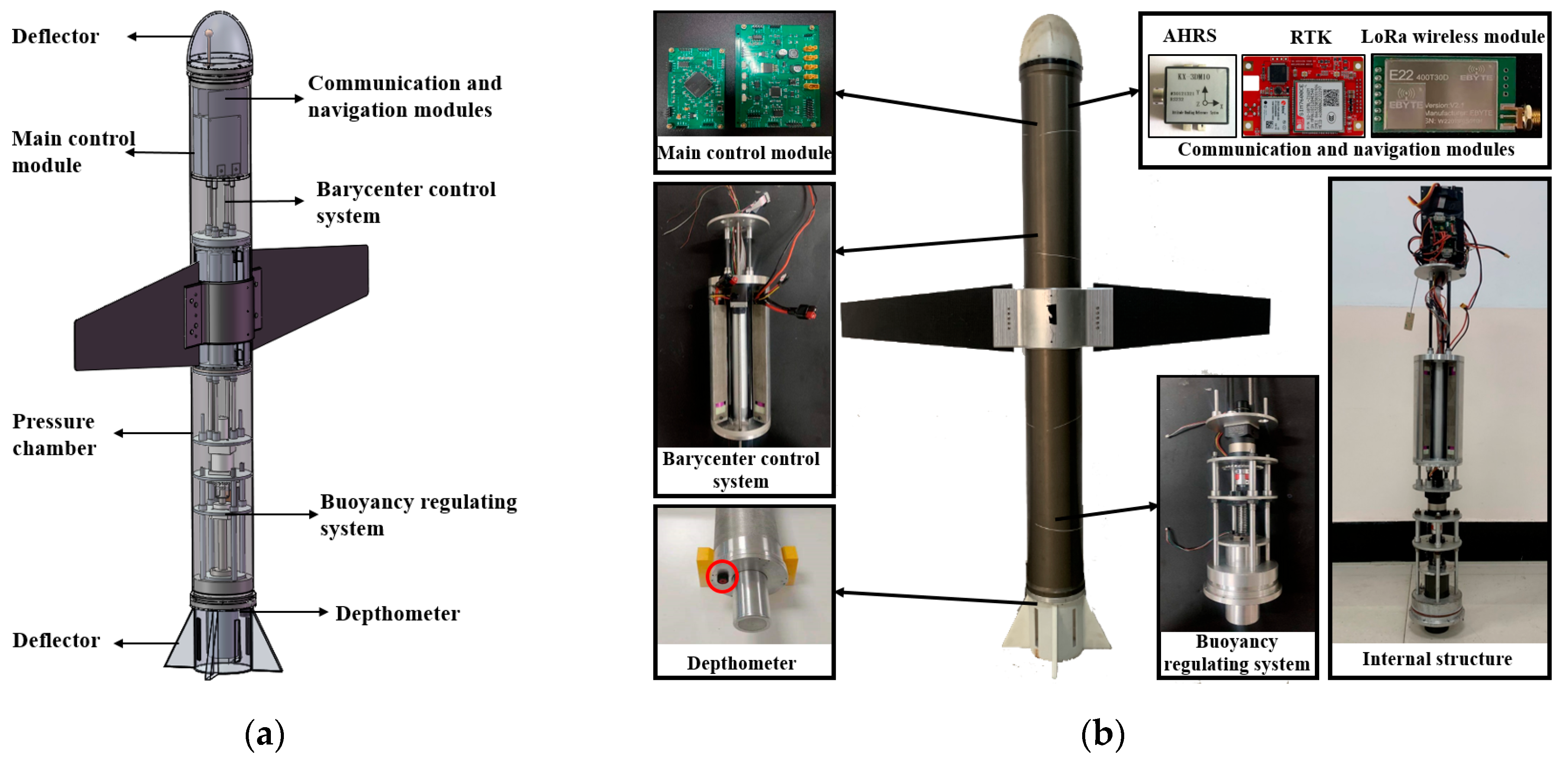
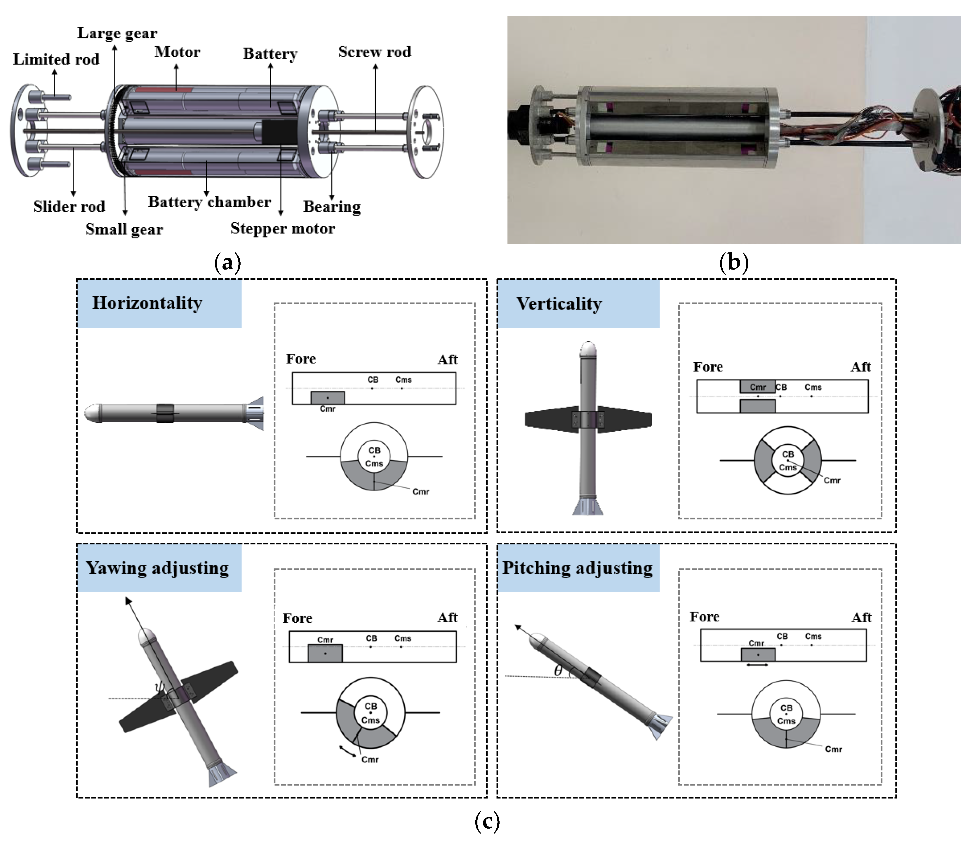
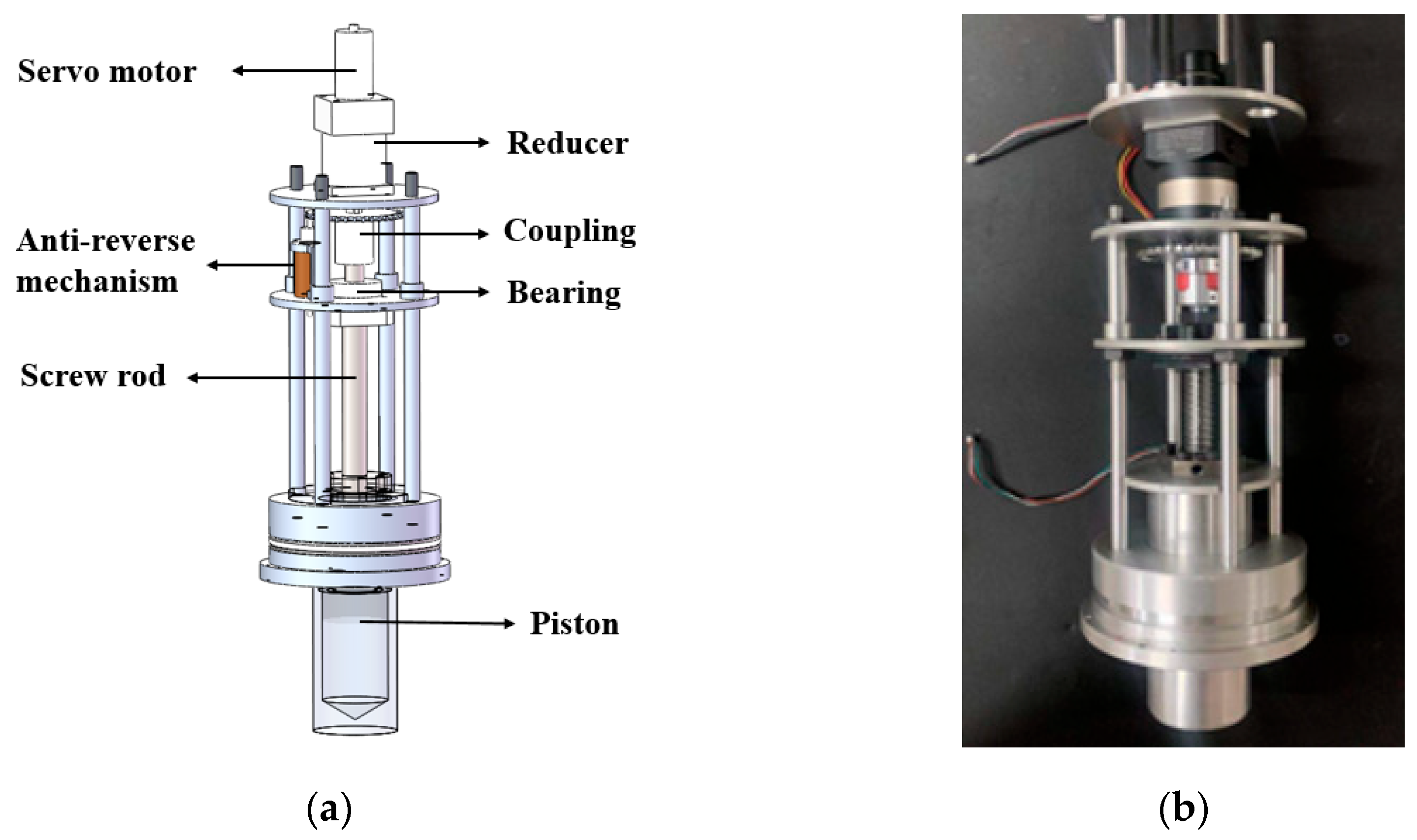
2.1. Structure of Miniaturized Underwater Profiler

The designated area persistent monitoring process of a miniaturized underwater profiler can be divided mainly into three stages: (1) vertical diving data acquisition; (2) gliding and floating upward displacement correction; and (3) sea surface positioning data transmission. The entire process is shown in Figure 1.

Based on the designated area persistent monitoring process, we designed a miniaturized underwater profiler (Figure 2). The overall underwater profiler system includes the following: pressure chamber, main control module, buoyancy regulating system, barycenter control system, communication module, navigation and positioning module, etc. The barycenter control system adjusts the motion posture of the miniaturized underwater profiler by controlling the position of the removable mass block. The buoyancy regulating system uses the piston’s extending and retracting to change the drainage volume of the miniaturized underwater profiler, thereby adjusting the net buoyancy and allowing the underwater profiler to rise or dive. The navigation module includes components such as gyroscopes, accelerometers, and magnetometers, which can provide information about the attitude angle, acceleration, and angular velocity of the miniaturized underwater profiler, providing data support for the obtainment of the underwater navigation information of the underwater profiler. In order to facilitate comparison, the main parameters of the miniaturized underwater profiler proposed in the study and the ZJU-HUP profiler described in [10] are shown in

Table 1. Main parameters of the miniaturized underwater profiler and ZJU-HUP profiler.

Parameters	Miniaturized Underwater Profiler 1	ZJU-HUP 2
Mass	11.25 kg	82 kg
Hull dimensions	Ø0.12 m × 1.2 m	Ø0.2377 m × 2.31 m
Buoyancy adjustment	0.3 L	1.8 L
Maximum dive depth	300 m	1200 m
Designated area persistent monitoring ability	<500 m	384 m
Buoyancy adjustment mode	Piston	Oil bladder

¹ Designed by the authors. ² Described in [10].

.

In order to adjust different angles when the miniaturized underwater profiler is diving or rising, the attitude adjustment system of the miniaturized underwater profiler must have greater angle adjustment capabilities. Compared with the traditional single mass block barycenter control method, the dual mass block barycenter control system has a wider range of attitude angle adjustments. Given the internal space of the underwater profiler, the battery pack can be used as the barycenter control mass block. The position of the gravity center of the miniaturized underwater profiler is controlled by driving the mass block to translate and rotate, thereby adjusting the attitude of the underwater profiler. The structure and regulation principle of dual mass block barycenter control system are shown in Figure 3.

The miniaturized underwater profiler has no propeller or other power-driving device, therefore, the buoyancy regulating system is the key to the entire observing movement, which provides upward/downward force. Considering the miniaturization requirements of underwater profilers, a variable volume method is chosen for net buoyancy adjustment. We have designed a piston-type buoyancy regulating system which uses a serve motor to drive the screw rotation and push the piston motion. Consequently, the requirement of changing the overall drainage volume of the profiler can be achieved. The buoyancy regulating system of the miniaturized underwater profiler is shown in Figure 4.

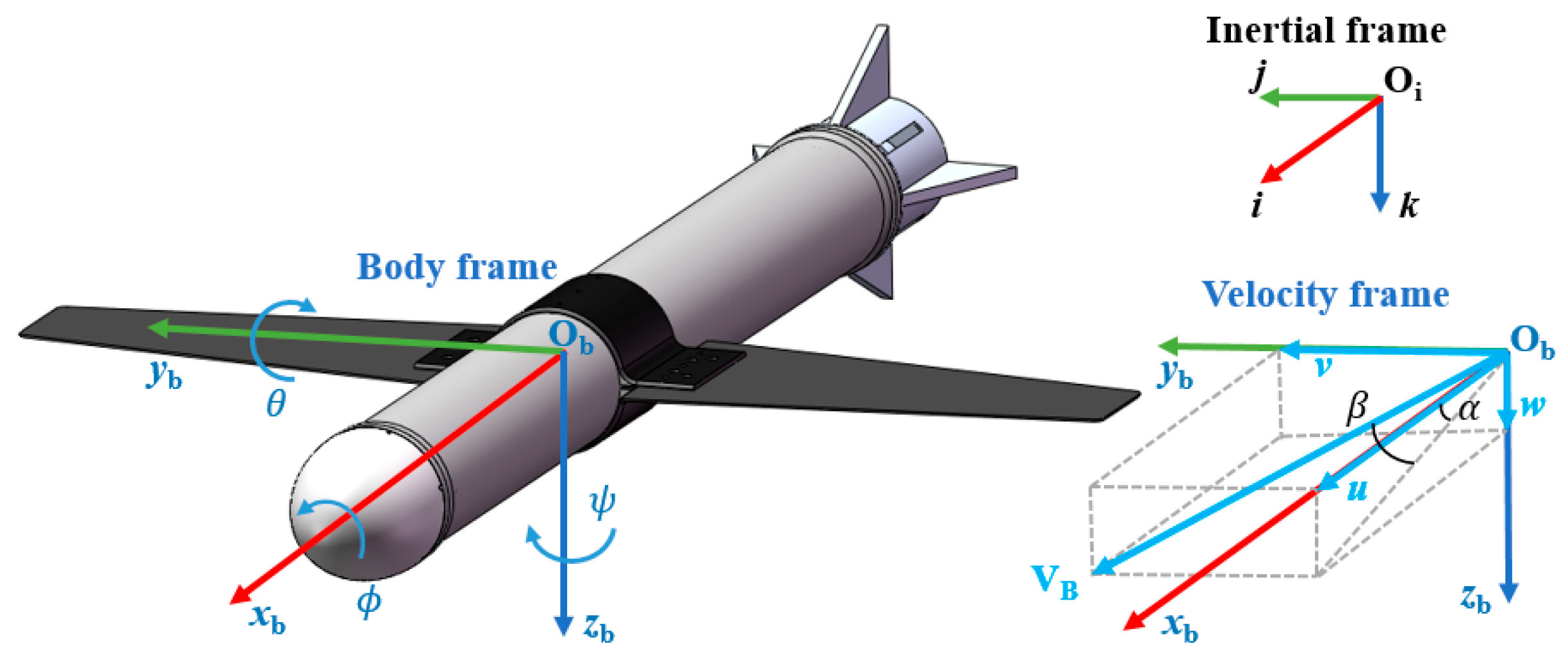
2.2. Kinematic and Dynamic Modeling of the Miniaturized Underwater Profiler

Based on the motion form of the miniaturized underwater profiler, the relevant coordinate system of the miniaturized underwater profiler is established. The defined coordinate system is shown in Figure 5.

The position and attitude of the miniaturized underwater profiler in the inertial coordinate system can be expressed as follows: ${\mathit{X}}_I={\left[x,y,z\right]}^T$ and $\mathit{\Theta }={\left[\varphi ,\theta ,\psi \right]}^T$, where x, y, and z represent respective position information and $\varphi$, $\theta$, and $\psi$ represent roll, pitch, and yaw angles, respectively. The linear and angular velocities of the miniaturized underwater profiler in the body coordinate system can be expressed as follows: ${\mathit{V}}_B={\left[u,v,w\right]}^T$ and $\mathit{\Omega }={\left[p,q,r\right]}^T$, in order to facilitate the calculation of viscous hydrodynamic forces and moments for the miniaturized underwater profiler, as well as to describe the relationship between the motion direction of the miniaturized underwater profiler and the body coordinate system. In the velocity coordinate system, the angle of attack can be expressed as $\alpha =\mathit{arctan}\left(\frac{w}{u}\right)$ and the drift angle can be expressed as $\beta =\mathit{arcsin}\left(\frac{v}{u^2+v^2+w^2}\right)$.

The velocity relationship of the miniaturized underwater profiler in the body coordinate system and the inertial coordinate system can be expressed as follows:

$$\begin{gathered} {\dot{\mathit{X}}}_I={\mathit{R}}_B^I\left(\mathit{\Theta }\right){\mathit{V}}_B \\ \dot{\mathit{\Theta }}={\mathit{J}}_B^I\left(\mathit{\Theta }\right)\mathit{\Omega } \end{gathered}$$

(1)

where ${\mathit{R}}_B^I\left(\mathit{\Theta }\right)=\left[\begin{array}{ccc}c\theta c\psi & s\varphi s\theta c\psi -c\varphi s\psi & c\varphi s\theta c\psi +s\varphi s\psi \\ c\theta s\psi & s\varphi s\theta s\psi +c\varphi c\psi & c\varphi s\theta s\psi -s\varphi c\psi \\ -s\theta & s\varphi c\theta & c\varphi c\theta \end{array}\right]$, ${\mathit{J}}_B^I\left(\mathit{\Theta }\right)=\frac{1}{c\theta }\left[\begin{array}{ccc}1& s\varphi s\theta & c\varphi s\theta \\ 0& c\varphi c\theta & -s\varphi c\theta \\ 0& s\varphi & c\varphi \end{array}\right]$, and the relevant symbols are abbreviated with $c=\mathit{cos}()$ and $s=\mathit{sin}()$.

The translational momentum of the miniaturized underwater profiler in the inertial coordinate system is defined as $\mathit{p}$ and the angular momentum is $\mathit{\pi }$. According to Newton’s law, the derivative of momentum over time is used to obtain the relationship between the external force and external moment that the miniaturized underwater profiler is subjected to in the inertial coordinate system, as follows:

$$\begin{gathered} \dot{\mathit{p}}={\mathit{f}}_{ex}+\left(m_s+m_d+m_b-\Delta m\right)g\mathit{k} \\ \dot{\mathit{\pi }}={\mathit{\tau }}_{ex}+m_{s}g\mathit{k}\times {\mathit{q}}_s+m_{d}g\mathit{k}\times {\mathit{q}}_d+m_{b}g\mathit{k}\times {\mathit{q}}_b \end{gathered}$$

(2)

where ${\mathit{f}}_{ex}$ and ${\mathit{\tau }}_{ex}$ are the external forces and the moments exerted by the external environment on the miniaturized underwater profiler, respectively; $m_s$, $m_d$, $m_b$, and $\Delta m$ represent the static mass, removable mass, adjustable buoyancy mass, and drainage mass of the miniaturized underwater profiler, respectively; ${\mathit{q}}_s$, ${\mathit{q}}_d$, and ${\mathit{q}}_b$ represent the positions of the static mass center of gravity, the removable mass center of gravity, and the net buoyancy center of the miniaturized underwater profiler in the inertial coordinate system, respectively; and $g$ is the magnitude of local gravitational acceleration. The unit vector $\mathit{k}$ pointing towards the direction of gravity in the inertial coordinate system.

$\mathit{P}$ and $\mathit{\Pi }$ represent the translational and angular momentums of the miniaturized underwater profiler in the body coordinate system, respectively. The following relationship between the translational and angular momentums in the inertial coordinate system and the body coordinate system are as follows:

$$\begin{gathered} \mathit{p}={\mathit{R}}_B^I\left(\mathit{\Theta }\right)\mathit{P} \\ \mathit{\pi }={\mathit{R}}_B^I\left(\mathit{\Theta }\right)\mathit{\Pi }+{\mathit{X}}_I\times \mathit{p} \end{gathered}$$

(3)

Take the derivative of Equation (3) to obtain the following:

$$\begin{gathered} \dot{\mathit{p}}={\mathit{R}}_B^I\left(\mathit{\Theta }\right)\left(\dot{\mathit{P}}+\mathit{\Omega }\mathit{P}\right) \\ \dot{\mathit{\pi }}={\mathit{R}}_B^I\left(\mathit{\Theta }\right)\left(\dot{\mathit{\Pi }}+\mathit{\Omega }\mathit{\Pi }\right)+{\mathit{R}}_B^I\left(\mathit{\Theta }\right){\mathit{V}}_B\times \mathit{p}+{\mathit{X}}_I\times \dot{\mathit{p}} \end{gathered}$$

(4)

By combining Equations (2) and (4), the following can be concluded:

$$\begin{gathered} \dot{\mathit{P}}=\mathit{P}\times \mathit{\Omega }+m_{b}g\left({\mathit{R}}_B^I{\left(\mathit{\Theta }\right)}^T\mathit{k}\right)+{\mathit{R}}_B^I{\left(\mathit{\Theta }\right)}^T{\mathit{f}}_{ex} \\ \dot{\mathit{\Pi }}=\mathit{\Pi }\times \mathit{\Omega }+\mathit{P}\times {\mathit{V}}_B+\left(m_s{\mathit{r}}_s+m_d{\mathit{r}}_d+m_b{\mathit{r}}_b\right)g\times \left({\mathit{R}}_B^I{\left(\mathit{\Theta }\right)}^T\mathit{k}\right)+{\mathit{R}}_B^I{\left(\mathit{\Theta }\right)}^T{\mathit{\tau }}_{ex} \end{gathered}$$

(5)

where, ${\mathit{r}}_s$, ${\mathit{r}}_d$, and ${\mathit{r}}_b$ are the positions of the static mass center of gravity, removable mass center of gravity, and net buoyancy center of the miniaturized underwater profiler in the body coordinate system, respectively.

The generalized relative velocity of the miniaturized underwater profiler in the body coordinate system is defined as ${\mathit{V}}_g$, which can be expressed as follows:

$${\mathit{V}}_g=\left[\begin{array}{c}{\mathit{V}}_B\\ \mathit{\Omega }\end{array}\right]$$

(6)

The generalized momentum of the miniaturized underwater profiler in the body coordinate system can be expressed as follows:

$$\mathit{\eta }=\left[\begin{array}{c}\mathit{P}\\ \mathit{\Pi }\end{array}\right]=\mathit{M}{\mathit{V}}_g$$

(7)

where $\mathit{M}$ is the generalized inertia matrix.

By taking the derivative on both sides of Equation (7), the following can be concluded:

$$\dot{\mathit{\eta }}=\left[\begin{array}{c}\dot{\mathit{P}}\\ \dot{\mathit{\Pi }}\end{array}\right]=\mathit{M}{\dot{\mathit{V}}}_g+\dot{\mathit{M}}{\mathit{V}}_g$$

(8)

Equation (8) can be rewritten as follows:

$${\dot{\mathit{V}}}_g=\left[\begin{array}{c}{\dot{\mathit{V}}}_B\\ \dot{\mathit{\Omega }}\end{array}\right]={\mathit{M}}^{-1}\left(\dot{\mathit{\eta }}-\dot{\mathit{M}}{\mathit{V}}_g\right)$$

(9)

By substituting Equations (5) and (8) into Equation (9), we can obtain the dynamic model of the miniaturized underwater profiler, as follows:

$${\dot{\mathit{V}}}_g={\mathit{M}}^{-1}\left\{-\dot{\mathit{M}}{\mathit{V}}_g+\left[\begin{array}{c}\mathit{P}\times \mathit{\Omega }+m_{b}g\left({\mathit{R}}_B^I{\left(\mathit{\Theta }\right)}^T\mathit{k}\right)+{\mathit{R}}_B^I{\left(\mathit{\Theta }\right)}^T{\mathit{f}}_{ex}\\ \mathit{\Pi }\times \mathit{\Omega }+\mathit{P}\times {\mathit{V}}_B+\left(m_s{\mathit{r}}_s+m_d{\mathit{r}}_d+m_b{\mathit{r}}_b\right)g\times \left({\mathit{R}}_B^I{\left(\mathit{\Theta }\right)}^T\mathit{k}\right)+{\mathit{R}}_B^I{\left(\mathit{\Theta }\right)}^T{\mathit{\tau }}_{ex}\end{array}\right]\right\}$$

(10)

where ${\mathit{F}}_B={\mathit{R}}_B^I{\left(\mathit{\Theta }\right)}^T{\mathit{f}}_{ex}$ and ${\mathit{T}}_B={\mathit{R}}_B^I{\left(\mathit{\Theta }\right)}^T{\mathit{\tau }}_{ex}$ can be used to represent the hydrodynamic forces and moments acting on the miniaturized underwater profiler in the body coordinate system.

The generalized inertia matrix $\mathit{M}$ can be represented as $\mathit{M}=\left[\begin{array}{cc}{\mathit{M}}_t& {\mathit{C}}_t\\ {\mathit{C}}_t^T& {\mathit{I}}_t\end{array}\right]$, where each part has the following relationships:

$$\begin{gathered} {\mathit{M}}_t=\left(m_s+m_d\right){\mathit{I}}_3+{\mathit{M}}_A \\ {\mathit{C}}_t={\mathit{C}}_A-m_s{\widehat{\mathit{r}}}_s-m_d{\widehat{\mathit{r}}}_d \\ {\mathit{I}}_t={\mathit{I}}_s+{\mathit{I}}_d+{\mathit{I}}_A-m_s{\widehat{\mathit{r}}}_s{\widehat{\mathit{r}}}_s-m_d{\widehat{\mathit{r}}}_d{\widehat{\mathit{r}}}_d \end{gathered}$$

(11)

where ${\mathit{I}}_3$ represents a $3\times 3$ unit matrix; ${\mathit{I}}_s$ and ${\mathit{I}}_d$ represent the moment of inertia of the static mass and the moment of inertia of the removable mass of the miniaturized underwater profiler in the body coordinate system, respectively; $\widehat{·}$ represents the antisymmetric matrix and exists as $\widehat{\mathit{x}}\mathit{y}=\mathit{x}\times \mathit{y}$ for the three-dimensional vectors $\mathit{x}$ and $\mathit{y}$; ${\mathit{M}}_A$, ${\mathit{C}}_A$ and ${\mathit{I}}_A$ are the additional mass, hydrodynamic coupling term, and additional moment of inertia of the miniaturized underwater profiler, respectively.

3. Dead Reckoning Algorithm of the Miniaturized Underwater Profiler

Miniaturized underwater profilers are susceptible to the influence of uncertain disturbances during the observation process, resulting in a gradual increase in the horizontal displacement and in the profilers moving away from the positioning center, leading to the failure of the designated area persistent monitoring task. In order to keep the miniaturized underwater profiler closer to the positioning center after gliding and floating upward, it is necessary to make decisions on the gliding angle and yaw angle of the miniaturized underwater profiler. Therefore, it is of primary importance to effectively obtain the navigation information of the miniaturized underwater profiler before making decisions. However, under the existing conditions, it is not possible to directly obtain the navigation information of the miniaturized underwater profiler, and this can only be obtained through dead reckoning. Additionally, it is necessary to improve the accuracy of dead reckoning.

3.1. State Equation and Observation Equation of the Miniaturized Underwater Profiler

In order to use the Kalman filter for underwater dead reckoning, the state equation and the observation equation of the miniaturized underwater profiler, based on its dynamical model, are established as follows:

$$\begin{array}{c}{\mathit{\chi }}_k=\mathit{F}\left({\mathit{\chi }}_{k-1},{\mathit{u}}_{k-1}\right)+{\mathit{\kappa }}_{k-1}\\ {\mathit{\gamma }}_k=\mathit{H}\left({\mathit{\chi }}_k\right)+{\mathit{\varsigma }}_k\end{array}$$

(12)

The input ${\mathit{u}}_{k-1}$ includes the underwater net buoyancy and hydrodynamic force at the $k-1$ moment of the miniaturized underwater profiler. ${\mathit{\kappa }}_{k-1}\in N(0,\mathit{Q})$ represents the process noise at the $k-1$ moment, and ${\mathit{\varsigma }}_k\in N(0,\mathit{R})$ represents the observation noise at the $k$ moment, both of these satisfy a normal distribution.

Considering the observability of the miniaturized underwater profiler system at the $k$ moment, the position ${\mathit{X}}_{I,k}$ and attitude angle ${\mathit{\Theta }}_k$ of the miniaturized underwater profiler in the inertial coordinate system, as well as the linear velocity ${\mathit{V}}_{B,k}$ and angular velocity ${\mathit{\Omega }}_k$ of the motion of the miniaturized underwater profiler in the body coordinate system, are selected as the state vectors. The specific form of ${\mathit{\chi }}_k$ can be expressed as follows:

$${\mathit{\chi }}_k={\left[{\mathit{X}}_{I,k}^T,{\mathit{\Theta }}_k^T,{\mathit{V}}_{B,k}^T,{\mathit{\Omega }}_k^T\right]}^T$$

(13)

By combining the state space Equations (12) and (13), the following can be concluded:

$${\mathit{\chi }}_k=\left[\begin{array}{cccc}{\mathit{I}}_3& {\mathit{O}}_3& {\mathit{R}}_B^I\left({\mathit{\Theta }}_{k-1}\right)\mathrm{\Delta }T& {\mathit{O}}_3\\ {\mathit{O}}_3& {\mathit{I}}_3& {\mathit{O}}_3& {\mathit{J}}_B^I\left({\mathit{\Theta }}_{k-1}\right)\mathrm{\Delta }T\\ {\mathit{O}}_3& {\mathit{O}}_3& {\mathit{I}}_3& {\mathit{O}}_3\\ {\mathit{O}}_3& {\mathit{O}}_3& {\mathit{O}}_3& {\mathit{I}}_3\end{array}\right]{\mathit{\chi }}_{k-1}+\left[\begin{array}{c}\frac{{\mathit{a}}_{k-1}\mathrm{\Delta }{T}^2}{2}\\ {\mathit{O}}_{3\times 1}\\ {\mathit{a}}_{k-1}\mathrm{\Delta }T\\ {\mathit{O}}_{3\times 1}\end{array}\right]+{\mathit{\kappa }}_{k-1}$$

(14)

where $\mathrm{\Delta }T$ is the sampling interval time and ${\mathit{a}}_{k-1}$ is the total acceleration generated by the underwater net buoyancy and hydrodynamic factors of the miniaturized underwater profiler system at the $k-1$ moment.

The sensors used for underwater dead reckoning in the miniaturized underwater profiler include micro attitude reference systems and depthometers. The micro attitude reference system can provide information on the attitude angle changes of the miniaturized underwater profiler. The depthometer can provide the information of depth and its variation. Attitude angle data can be obtained through attitude angle calculation methods. Based on the data obtained from sensor and attitude angle calculation, the observation vector is selected as follows:

$${\mathit{\gamma }}_k={\left[z_k,{\mathit{\Theta }}_k^T,{\dot{\mathit{X}}}_{I,k}^T,{\mathit{\Omega }}_k^T\right]}^T$$

(15)

During the floating upward process of the miniaturized underwater profiler, a certain pitch angle is required for the gliding motion in order to correct the errors caused by uncertain disturbance. At the same time, the sensors carried by the miniaturized underwater profiler have a higher frequency of information sampling. Consequently, it can be approximated that the miniaturized underwater profiler strictly performs the gliding motion in each cycle. Therefore, based on the data $z_k$ collected by the depthometer in the depth direction, ${\dot{z}}_k$ can be obtained and, when combined with the calculated attitude angle information, ${\dot{x}}_k$ and ${\dot{y}}_k$ at the $k$ moment can be inferred as follows:

$$\begin{gathered} {\dot{x}}_k=\frac{{\dot{z}}_k}{\mathit{tan}{\theta }_k}\mathit{cos}{\psi }_k \\ {\dot{y}}_k=\frac{{\dot{z}}_k}{\mathit{tan}{\theta }_k}\mathit{sin}{\psi }_k \end{gathered}$$

(16)

Therefore, from Equations (1) and (12), the following can be obtained:

$${\mathit{\gamma }}_k=\left[\begin{array}{cccc}\left[0,0,1\right]& {\mathit{O}}_{1\times 3}& {\mathit{O}}_{1\times 3}& {\mathit{O}}_{1\times 3}\\ {\mathit{O}}_3& {\mathit{I}}_3& {\mathit{O}}_3& {\mathit{O}}_3\\ {\mathit{O}}_3& {\mathit{O}}_3& {\mathit{R}}_B^I\left({\mathit{\Theta }}_k\right)& {\mathit{O}}_3\\ {\mathit{O}}_3& {\mathit{O}}_3& {\mathit{O}}_3& {\mathit{I}}_3\end{array}\right]{\mathit{\chi }}_k+{\mathit{\varsigma }}_k$$

(17)

3.2. Extended Kalman Filter, Unscented Kalman Filter, and Cubature Kalman Filter

3.2.1. Extended Kalman Filter

The EKF is one of the most employed nonlinear filtering approaches and is still currently applied. The EKF algorithm includes two main steps, time update and measurement update.

• Filter initialization

$$\begin{gathered} {\widehat{\mathit{\chi }}}_0=E\left\{{\mathit{\chi }}_0\right\} \\ {\widehat{\mathit{P}}}_0=E\left\{\left[({\mathit{\chi }}_0-{\widehat{\mathit{\chi }}}_0)({\mathit{\chi }}_0-{\widehat{\mathit{\chi }}}_0{)}^T\right]\right\} \end{gathered}$$

(18)

where ${\widehat{\mathit{P}}}_0$ represents the error covariance matrix of the estimated state vector. Setting $\mathrm{k}\in \left\{1,\dots ,m\right\}$.

2.

Time update

Compute the partial derivative matrix:

$${\mathit{F}}_{k-1}={\left.\frac{\partial \mathit{F}\left(\mathit{\chi }\right)}{\partial \mathit{\chi }}\right|}_{{\widehat{\mathit{\chi }}}_{k-1}}$$

(19)

Estimate the propagated state and covariance matrix for instant k:

$$\begin{gathered} {\overline{\mathit{\chi }}}_k=\mathit{F}\left({\widehat{\mathit{\chi }}}_{k-1}\right) \\ {\overline{\mathit{P}}}_k={\mathit{F}}_{k-1}{\widehat{\mathit{P}}}_{k-1}{\mathit{F}}_{k-1}^T+{\mathit{Q}}_{k-1} \end{gathered}$$

(20)

3.

Measurement update

Compute the partial derivative matrix:

$${\mathit{H}}_k={\left.\frac{\partial \mathit{H}\left(\mathit{\chi }\right)}{\partial \mathit{\chi }}\right|}_{{\overline{\mathit{\chi }}}_k}$$

(21)

Estimate the Kalman gain, update state and covariance matrix:

$$\begin{gathered} {\mathit{K}}_k={\overline{\mathit{P}}}_k{\mathit{H}}_k^T{\left({\mathit{H}}_k{\overline{\mathit{P}}}_k{\mathit{H}}_k^T+{\mathit{R}}_k\right)}^{-1} \\ {\widehat{\mathit{\chi }}}_k={\overline{\mathit{\chi }}}_k+{\mathit{K}}_k\left[{\mathit{\gamma }}_k-\mathit{H}\left({\overline{\mathit{\chi }}}_k\right)\right] \\ {\widehat{\mathit{P}}}_k=\left(\mathit{I}-{\mathit{K}}_k{\mathit{H}}_k\right){\overline{\mathit{P}}}_k \end{gathered}$$

(22)

3.2.2. Unscented Kalman Filter

UKF can reduce the linearization errors of the EKF. The UKF algorithm has the following steps.

• Filter initialization

The procedure is the same as that in Equation (18).

2.

Time update

Generate the sigma points ${\mathit{\chi }}_{i,k-1}(i=0,1,\dots ,2n)$:

$$\begin{gathered} {\mathit{\chi }}_{0,k-1}={\widehat{\mathit{\chi }}}_{k-1},i=0 \\ {\mathit{\chi }}_{i,k-1}={\widehat{\mathit{\chi }}}_{k-1}+{\left(\sqrt{\left(n+\lambda \right){\widehat{\mathit{P}}}_{k-1}}\right)}_i, i=1,\dots ,n \\ {\mathit{\chi }}_{i,k-1}={\widehat{\mathit{\chi }}}_{k-1}-{\left(\sqrt{(n+\lambda ){\widehat{\mathit{P}}}_{k-1}}\right)}_{i-n},i=n+1,\dots ,2n \end{gathered}$$

(23)

where $\lambda$ is a scaling parameter.

Propagation of sigma points:

$${\overline{\mathit{\chi }}}_{i,k}=\mathit{F}\left({\mathit{\chi }}_{i,k-1}\right),i=0,\dots ,2n$$

(24)

Estimation of the propagated state and covariance matrix for instant k:

$${\overline{\mathit{\chi }}}_k=\frac{\lambda }{n+\lambda }{\overline{\mathit{\chi }}}_{0,k}+\sum _{i=1}^{2n}\frac{1}{2\left(n+\lambda \right)}{\overline{\mathit{\chi }}}_{i,k}$$

(25)

$${\overline{\mathit{P}}}_k=\frac{\lambda }{n+\lambda }\left[{\overline{\mathit{\chi }}}_{0,k}-{\overline{\mathit{\chi }}}_k\right]{\left[{\overline{\mathit{\chi }}}_{0,k}-{\overline{\mathit{\chi }}}_k\right]}^T+\sum _{i=1}^{2n}\frac{1}{2\left(n+\lambda \right)}\left[{\overline{\mathit{\chi }}}_{i,k}-{\overline{\mathit{\chi }}}_k\right]{\left[{\overline{\mathit{\chi }}}_{i,k}-{\overline{\mathit{\chi }}}_k\right]}^T+{\mathit{Q}}_{k-1}$$

(26)

3.

Measurement update

Evaluation of the sigma points: ${\mathit{\chi }}_{i,k-1}(i=0,1,\dots ,2n)$:

$$\begin{gathered} {\mathit{\chi }}_{0,k}={\overline{\mathit{\chi }}}_k,i=0 \\ {\mathit{\chi }}_{i,k}={\overline{\mathit{\chi }}}_k+{\left(\sqrt{\left(n+\lambda \right){\overline{\mathit{P}}}_k}\right)}_i, i=1,\dots ,n \\ {\mathit{\chi }}_{i,k}={\overline{\mathit{\chi }}}_k-{\left(\sqrt{(n+\lambda ){\overline{\mathit{P}}}_k}\right)}_{i-n},i=n+1,\dots ,2n \end{gathered}$$

(27)

Propagation of the sigma points through the measurement model:

$${\mathit{\gamma }}_{i,k}=\mathit{H}\left({\mathit{\chi }}_{i,k}\right),i=0,\dots ,2n$$

(28)

Estimation of the predicted measurement, innovation covariance matrix and cross-covariance matrix:

$$\begin{gathered} {\overline{\mathit{\gamma }}}_k=\frac{\lambda }{n+\lambda }{\mathit{\gamma }}_{0,k}+\sum _{i=1}^{2n}\frac{1}{2\left(n+\lambda \right)}{\mathit{\gamma }}_{i,k} \\ {\mathit{P}}_{zz,k}=\frac{\lambda }{n+\lambda }\left[{\mathit{\gamma }}_{0,k}-{\overline{\mathit{\gamma }}}_k\right]{\left[{\mathit{\gamma }}_{0,k}-{\overline{\mathit{\gamma }}}_k\right]}^T+\sum _{i=1}^{2n}\frac{1}{2\left(n+\lambda \right)}\left[{\mathit{\gamma }}_{i,k}-{\overline{\mathit{\gamma }}}_k\right]{\left[{\mathit{\gamma }}_{i,k}-{\overline{\mathit{\gamma }}}_k\right]}^T+{\mathit{R}}_k \\ {\mathit{P}}_{xz,k}=\frac{\lambda }{n+\lambda }\left[{\overline{\mathit{\chi }}}_{0,k}-{\overline{\mathit{\chi }}}_k\right]{\left[{\mathit{\gamma }}_{0,k}-{\overline{\mathit{\gamma }}}_k\right]}^T+\sum _{i=1}^{2n}\frac{1}{2\left(n+\lambda \right)}\left[{\overline{\mathit{\chi }}}_{i,k}-{\overline{\mathit{\chi }}}_k\right]{\left[{\mathit{\gamma }}_{i,k}-{\overline{\mathit{\gamma }}}_k\right]}^T \end{gathered}$$

(29)

Estimation of the Kalman gain, update state and covariance matrix:

$$\begin{gathered} {\mathit{K}}_k={\mathit{P}}_{xz,k}{\left({\mathit{P}}_{zz,k}\right)}^{-1} \\ {\widehat{\mathit{\chi }}}_k={\overline{\mathit{\chi }}}_k+{\mathit{K}}_k\left[{\mathit{\gamma }}_k-{\overline{\mathit{\gamma }}}_k\right] \\ {\widehat{\mathit{P}}}_k={\overline{\mathit{P}}}_k-{\mathit{K}}_k{\mathit{P}}_{zz,k}{\mathit{K}}_k^T \end{gathered}$$

(30)

3.2.3. Cubature Kalman Filter

CKF uses a set of cubature points of equal weight to calculate the means and covariances of state variables which, after nonlinear transformation, yield a performance of nonlinear optimal approximation. The CKF algorithm has the following equations.

• Filter initialization

The procedure is also the same as that in Equation (18).

2.

Time update

Calculation of the cubature points ${\mathit{\chi }}_{i,k-1}(i=1,2,\dots ,2n)$:

$${\mathit{\chi }}_{i,k-1}=\sqrt{{\widehat{\mathit{P}}}_{k-1}}{\mathit{\xi }}_i+{\widehat{\mathit{\chi }}}_{k-1}$$

(31)

where ${\mathit{\xi }}_i$ is a set of cubature points, which can be expressed as follows:

$${\mathit{\xi }}_i=\left\{\begin{array}{c}\begin{array}{cc}\sqrt{n}{\left[1\right]}_i& i=1,\dots ,n\end{array}\\ \begin{array}{cc}-\sqrt{n}{\left[1\right]}_i& i=n+1,\dots ,2n\end{array}\end{array}\right.$$

(32)

Propagation of cubature points:

$${\overline{\mathit{\chi }}}_{i,k}=\mathit{F}\left({\mathit{\chi }}_{i,k-1}\right)$$

(33)

Estimation of the propagated state and covariance matrix for instant k:

$$\begin{gathered} {\overline{\mathit{\chi }}}_k=\frac{1}{2n}\sum _{i=1}^{2n}{\overline{\mathit{\chi }}}_{i,k} \\ {\overline{\mathit{P}}}_k=\frac{1}{2n}\sum _{i=1}^{2n}\left[{\overline{\mathit{\chi }}}_{i,k}{\overline{\mathit{\chi }}}_{i,k}^T\right]-{\overline{\mathit{\chi }}}_k{\overline{\mathit{\chi }}}_k^T+{\mathit{Q}}_{k-1} \end{gathered}$$

(34)

3.

Measurement update

Evaluation of the cubature points ${\mathit{\chi }}_{i,k}(i=1,2,\dots ,2n)$:

$${\mathit{\chi }}_{i,k}=\sqrt{{\overline{\mathit{P}}}_k}{\mathit{\xi }}_i+{\overline{\mathit{\chi }}}_k$$

(35)

Propagation of the cubature points through the measurement model:

$${\mathit{\gamma }}_{i,k}=\mathit{H}\left({\mathit{\chi }}_{i,k}\right)$$

(36)

Estimation of the predicted measurement, innovation covariance matrix and cross-covariance matrix:

$$\begin{gathered} {\overline{\mathit{\gamma }}}_k=\frac{1}{2n}\sum _{i=1}^{2n}{\mathit{\gamma }}_{i,k} \\ {\mathit{P}}_{zz,k}=\frac{1}{2n}\sum _{i=1}^{2n}\left[{\mathit{\gamma }}_{i,k}{\mathit{\gamma }}_{i,k}^T\right]-\left[{\overline{\mathit{\gamma }}}_k{\overline{\mathit{\gamma }}}_k^T\right]+{\mathit{R}}_k \\ {\mathit{P}}_{xz,k}=\frac{1}{2n}\sum _{i=1}^{2n}\left[{\mathit{\chi }}_{i,k}{\mathit{\gamma }}_{i,k}^T\right]-\left[{\overline{\mathit{\chi }}}_k{\overline{\mathit{\gamma }}}_k^T\right] \end{gathered}$$

(37)

Then, estimation of the Kalman gain, update state and covariance matrix are achieved in the same manner as in Equation (30).

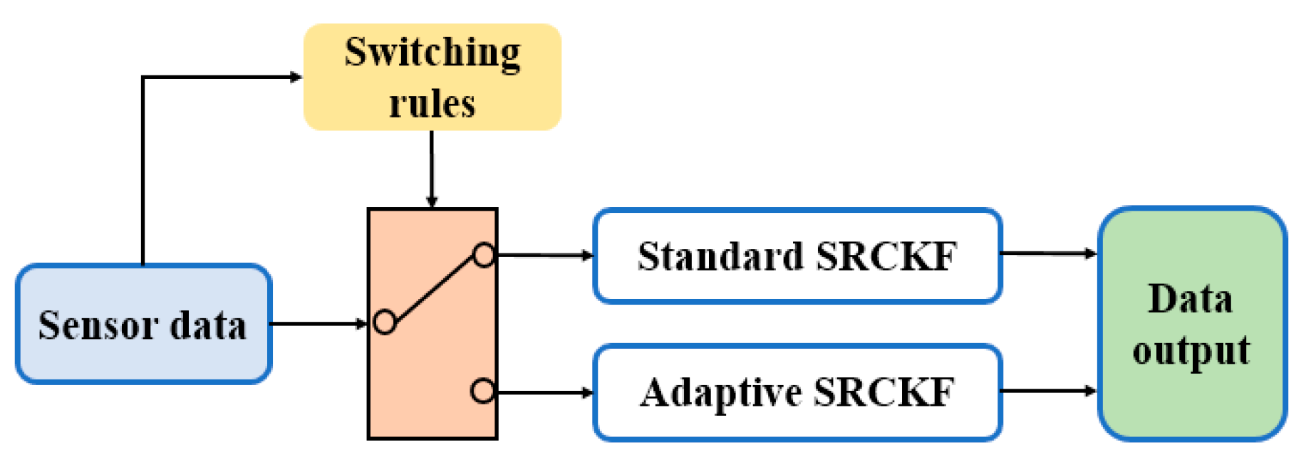
3.3. Dual-Mode Square Root Cubature Kalman Filter

3.3.1. Square Root Cubature Kalman Filter

The SRCKF algorithm ensures the symmetry and positive quality of the covariance matrix, avoids instability and divergence problems, and improves the calculation accuracy. In a miniaturized underwater profiler system, the SRCKF algorithm [31] is as follows.

• Filter initialization

Initialize the relevant parameters in the miniaturized underwater profiler system, the procedure is also the same as that in Equation (18), and perform Cholesky decomposition on the initial covariance matrix to obtain its square root initial value ${\mathit{S}}_0$:

$${\mathit{S}}_0=chol\left({\widehat{\mathit{P}}}_0\right)$$

(38)

where $\mathit{chol}()$ represents the decomposition of an any order matrix $\mathit{A}$ into a lower triangular matrix $\mathit{L}$, namely: $\mathit{A}=\mathit{L}{\mathit{L}}^T$.

2.

Time update

Step 1: Calculate the cubature points and bring the cubature points into the state equation of the miniaturized underwater profiler for propagation ($i=1,\dots ,2n)$:

$$\begin{gathered} {\mathit{\chi }}_{i,k-1}={\mathit{S}}_{k-1}{\mathit{\xi }}_i+{\widehat{\mathit{\chi }}}_{k-1} \\ {\mathit{\chi }}_{i,k}^{*}=\mathit{F}\left({\mathit{\chi }}_{i,k-1},{\mathit{u}}_{k-1}\right) \end{gathered}$$

(39)

where $n$ represents the dimension of the state vector and ${\mathit{\xi }}_i$ is a set of cubature points that defines in Equation (32).

Step 2: Calculate the predicted system state value at the $k$ moment:

$${\overline{\mathit{\chi }}}_k=\frac{1}{2n}{\displaystyle \sum _{i=1}^{2n}}{\mathit{\chi }}_{i,k}^{*}$$

(40)

Step 3: Calculate the square root of the predicted covariance matrix of the state error of the miniaturized underwater profiler:

$${\overline{\mathit{S}}}_k=tria\left\{\left[{\mathbf{\zeta }}_k^{*},{\mathit{S}}_{Q,k-1}\right]\right\}$$

(41)

where $\mathit{tria}()$ represents QR decomposition, which entails decomposing the matrix ${\mathit{A}}^T$ into an orthogonal matrix $\mathit{B}$ and an upper triangular matrix $\mathit{C}$, namely ${\mathit{C}}^T=tria\left(\mathit{A}\right)$; ${\mathit{S}}_{Q,k-1}$ is Cholesky decomposition of the process state noise ${\mathit{Q}}_{k-1}$ at the $k-1$ moment. ${\mathbf{\zeta }}_k^{*}$ and ${\mathit{S}}_{Q,k-1}$ can be represented as follows:

$$\begin{gathered} {\mathbf{\zeta }}_k^{*}=\frac{1}{\sqrt{2n}}\left[{\mathit{\chi }}_{1,k}^{*}-{\overline{\mathit{\chi }}}_k,{\mathit{\chi }}_{2,k}^{*}-{\overline{\mathit{\chi }}}_k,\dots ,{\mathit{\chi }}_{2n,k}^{*}-{\overline{\mathit{\chi }}}_k\right] \\ {\mathit{S}}_{Q,k-1}=chol({\mathit{Q}}_{k-1}) \end{gathered}$$

(42)

3.

Measurement update

Step 4: Recalculate the cubature points and bring the recalculated cubature point into the observation equation of the miniaturized underwater profiler for propagation $(i=1,2,\dots ,2n),$ as follows:

$$\begin{gathered} {\mathit{\chi }}_{i,k}={\overline{\mathit{S}}}_k{\mathit{\xi }}_i+{\overline{\mathit{\chi }}}_k \\ {\mathit{\gamma }}_{i,k}=\mathit{H}\left({\mathit{\chi }}_{i,k}\right) \end{gathered}$$

(43)

Step 5: Calculate the predicted measurement value, as follows:

$${\overline{\mathit{\gamma }}}_k=\frac{1}{2n}\sum _{i=1}^{2n}{\mathit{\gamma }}_{i,k}$$

(44)

Step 6: Calculate the square root of the covariance matrix of the measurement error of the miniaturized underwater profiler, as follows:

$${\mathit{S}}_{zz,k}=tria\left\{\left[{\mathit{\rho }}_k,{\mathit{S}}_{R,k}\right]\right\}$$

(45)

where ${\mathit{S}}_{R,k}$ is Cholesky decomposition of the measurement noise ${\mathit{R}}_k$ at the $k$ moment. ${\mathit{\rho }}_k$ and ${\mathit{S}}_{R,k}$ can be represented as follows:

$$\begin{gathered} {\mathit{\rho }}_k=\frac{1}{\sqrt{2n}}\left[{\mathit{\gamma }}_{1,k}-{\overline{\mathit{\gamma }}}_k,{\mathit{\gamma }}_{2,k}-{\overline{\mathit{\gamma }}}_k,\dots ,{\mathit{\gamma }}_{2n,k}-{\overline{\mathit{\gamma }}}_k\right] \\ {\mathit{S}}_{R,k}=chol({\mathit{R}}_k) \end{gathered}$$

(46)

The error covariance matrix ${\mathit{P}}_{zz,k}$ of the measurement value at the $k$ moment and the autocorrelation covariance matrix ${\mathit{P}}_{z,k}$ of the measurement value can be expressed as follows:

$$\begin{gathered} {\mathit{P}}_{zz,k}={\mathit{S}}_{zz,k}{\mathit{S}}_{zz,k}^T \\ {\mathit{P}}_{z,k}={\mathit{P}}_{zz,k}-{\mathit{R}}_k \end{gathered}$$

(47)

Step 7: Calculate the square root of the cross-correlation covariance matrix, as follows:

$${\mathit{P}}_{xz,k}={\mathbf{\zeta }}_k{\mathit{\rho }}_k^T$$

(48)

where ${\mathbf{\zeta }}_k$ can be expressed as follows:

$${\mathbf{\zeta }}_k=\frac{1}{\sqrt{2n}}\left[{\mathit{\chi }}_{1,k}-{\overline{\mathit{\chi }}}_k,{\mathit{\chi }}_{2,k}-{\overline{\mathit{\chi }}}_k,\dots ,{\mathit{\chi }}_{2n,k}-{\overline{\mathit{\chi }}}_k\right]$$

(49)

Step 8: Calculate the Kalman gain, the estimated value of the state vector at the $k$ moment, and the square root of the covariance matrix of the state error, as follows:

$$\begin{array}{c}{\mathit{K}}_k=({\mathit{P}}_{xz,k}/{\mathit{S}}_{zz,k}^T)/{\mathit{S}}_{zz,k}\\ {\widehat{\mathit{\chi }}}_k={\overline{\mathit{\chi }}}_k+{\mathit{K}}_k[{\mathit{\gamma }}_k-{\overline{\mathit{\gamma }}}_k]\\ {\mathit{S}}_k=tria\left\{\left[{\mathbf{\zeta }}_k-{\mathit{K}}_k{\mathit{\rho }}_k,{\mathit{K}}_k{\mathit{S}}_{R,k}\right]\right\}\end{array}$$

(50)

3.3.2. Adaptive Square Root Cubature Kalman Filter

The changes in measurement conditions have a significant impact on the standard SRCKF algorithm and the SRCKF algorithm does not have the ability to adapt to changes in measurement conditions. Therefore, in order to ensure that the SRCKF algorithm is robust against poor measurement values of the miniaturized underwater profiler, an adaptive SRCKF is proposed based on the state space model of the miniaturized underwater profiler.

The error value of the measurement at the $k$ moment of the miniaturized underwater profiler is ${\mathit{e}}_k={\mathit{\gamma }}_k-{\overline{\mathit{\gamma }}}_k$. According to Equation (47), there exists a relationship when the measured values of the system are normal, as follows:

$${\mathit{P}}_{zz,k}={\mathit{e}}_k{\mathit{e}}_k^T={\mathit{P}}_{z,k}+{\mathit{R}}_k$$

(51)

However, when the measured values of the system are poor, Equation (47) is not valid. An adaptive factor ${\mu }_k$ is introduced, and the above relationship can be rewritten as follows:

$${\mathit{P}}_{zz,k}={\mathit{P}}_{z,k}+{\mu }_k{\mathit{R}}_k$$

(52)

The square root of the covariance matrix of the measurement error becomes the following:

$${\mathit{S}}_{zz,k}=tria\left\{\left[{\mathit{\rho }}_k,\sqrt{{\mu }_k}{\mathit{S}}_{R,k}\right]\right\}$$

(53)

The square root of the covariance matrix of the state error is also changed to the following:

$${\mathit{S}}_k=tria\left\{\left[{\mathbf{\zeta }}_k-{\mathit{K}}_k{\mathit{\rho }}_k,{\mathit{K}}_k\sqrt{{\mu }_k}{\mathit{S}}_{R,k}\right]\right\}$$

(54)

The adaptive factor ${\mu }_k$ is as follows:

$${\mu }_k=\frac{{\mathit{e}}_k^T{\mathit{e}}_k-tr\left[{\mathit{P}}_{z,k}\right]}{tr\left[{\mathit{R}}_k\right]}$$

(55)

where $tr\left(\right)$ represents the trace operation.

3.3.3. Switching Rules

The filter structure of the underwater dead reckoning sensor system for the miniaturized underwater profiler is shown in Figure 6. When the measured values of the miniaturized underwater profiler system perform normally, the standard SRCKF algorithm is used and when the measured values of the system perform poorly, the adaptive SRCKF algorithm is used to infer the underwater position and attitude of the miniaturized underwater profiler.

In order to establish switching rules for filters, a statistical function for the quality detection of data values measured by miniaturized underwater profilers is introduced, as follows:

$${\beta }_k={\mathit{e}}_k^T{\left[{\mathit{P}}_{zz,k}\right]}^{-1}{\mathit{e}}_k$$

(56)

The statistical function satisfies condition ${\beta }_k~{\chi }^2\left(n\right)$, the chi-square distribution with degree of freedom $n$; $n$ is the dimension of the measurement error vector ${\mathit{e}}_k$ of the miniaturized underwater profiler. Determine the threshold ${\chi }_{\delta ,M}^2$ for data quality detection based on the accuracy $\delta$ of data quality control, as follows:

$$P\left\{{\chi }^2>{\chi }_{\delta ,M}^2\right\}=\delta$$

(57)

Develop switching rules for standard SRCKF and adaptive SRCKF filters, as follows: (1) when ${\beta }_k\le {\chi }_{\delta ,M}^2$ considers the measured value to be in a normal state, select the standard SRCKF algorithm and (2) when ${\beta }_k>{\chi }_{\delta ,M}^2$ considers the measured values to be in a poor state, the adaptive SRCKF algorithm is chosen.

The DSRCKF algorithm is illustrated by the pseudocode in Algorithm 1.

Algorithm 1. dual-mode square root cubature Kalman filter

Input: ${\widehat{\mathit{\chi }}}_{k-1}$, ${\mathit{u}}_{k-1}$, ${\mathit{Q}}_{k-1}$, ${\mathit{R}}_k$, ${\mathit{S}}_{k-1}$ Output: ${\widehat{\mathit{\chi }}}_k$, ${\mathit{S}}_k$

1: Setting number of cycles m 2: Filter initialization 3: ${\widehat{\mathit{\chi }}}_0$, ${\widehat{\mathit{P}}}_0$, ${\mathit{S}}_0$ 4: while k ≤ m do 5:  Time update 6:   ${\mathit{\chi }}_{i,k-1}={\mathit{S}}_{k-1}{\mathit{\xi }}_i+{\widehat{\mathit{\chi }}}_{k-1}$, ${\mathit{\chi }}_{i,k}^{*}=\mathit{F}\left({\mathit{\chi }}_{i,k-1},{\mathit{u}}_{k-1}\right)$ 7:   ${\overline{\mathit{\chi }}}_k=\frac{1}{2n}{\sum }_{i=1}^{2n}{\mathit{\chi }}_{i,k}^{*}$ 8:   ${\mathbf{\zeta }}_k^{*}=\frac{1}{\sqrt{2n}}\left[{\mathit{\chi }}_{1,k}^{*}-{\overline{\mathit{\chi }}}_k,{\mathit{\chi }}_{2,k}^{*}-{\overline{\mathit{\chi }}}_k,\dots ,{\mathit{\chi }}_{2n,k}^{*}-{\overline{\mathit{\chi }}}_k\right]$, ${\mathit{S}}_{Q,k-1}=chol\left({\mathit{Q}}_{k-1}\right)$ 9:   ${\overline{\mathit{S}}}_k=tria\left\{\left[{\mathbf{\zeta }}_k^{*},{\mathit{S}}_{Q,k-1}\right]\right\}$ 10:  Measurement update 11:   ${\mathit{\chi }}_{i,k}={\overline{\mathit{S}}}_k{\mathit{\xi }}_i+{\overline{\mathit{\chi }}}_k$, ${\mathit{\gamma }}_{i,k}=\mathit{H}\left({\mathit{\chi }}_{i,k}\right)$ 12:   ${\overline{\mathit{\gamma }}}_k=\frac{1}{2n}{\sum }_{i=1}^{2n}{\mathit{\gamma }}_{i,k}$ 13:   ${\mathit{\rho }}_k=\frac{1}{\sqrt{2n}}\left[{\mathit{\gamma }}_{1,k}-{\overline{\mathit{\gamma }}}_k,{\mathit{\gamma }}_{2,k}-{\overline{\mathit{\gamma }}}_k,\dots ,{\mathit{\gamma }}_{2n,k}-{\overline{\mathit{\gamma }}}_k\right]$, ${\mathit{S}}_{R,k}=chol\left({\mathit{R}}_k\right)$ 14:   ${\mathit{S}}_{zz,k}=tria\left\{\left[{\mathit{\rho }}_k,{\mathit{S}}_{R,k}\right]\right\}$, ${\mathit{P}}_{zz,k}={\mathit{S}}_{zz,k}{\mathit{S}}_{zz,k}^T$, ${\mathit{P}}_{z,k}={\mathit{P}}_{zz,k}-{\mathit{R}}_k$ 15:   ${\mathbf{\zeta }}_k=\frac{1}{\sqrt{2n}}\left[{\mathit{\chi }}_{1,k}-{\overline{\mathit{\chi }}}_k,{\mathit{\chi }}_{2,k}-{\overline{\mathit{\chi }}}_k,\dots ,{\mathit{\chi }}_{2n,k}-{\overline{\mathit{\chi }}}_k\right]$ 16:   ${\mathit{P}}_{xz,k}={\mathbf{\zeta }}_k{\mathit{\rho }}_k^T$ 17:  Switching 18:   ${\mathit{e}}_k={\mathit{\gamma }}_k-{\overline{\mathit{\gamma }}}_k$, ${\beta }_k={\mathit{e}}_k^T{\left[{\mathit{P}}_{zz,k}\right]}^{-1}{\mathit{e}}_k$ 19:   ${\beta }_k~{\chi }^2\left(n\right)$, $P\left\{{\chi }^2>{\chi }_{\delta ,M}^2\right\}=\delta$ 20:   if ${\beta }_k\le {\chi }_{\delta ,M}^2$ then standard SRCKF 21:    ${\mathit{S}}_k=tria\left\{\left[{\mathbf{\zeta }}_k-{\mathit{K}}_k{\mathit{\rho }}_k,{\mathit{K}}_k{\mathit{S}}_{R,k}\right]\right\}$ 22:   else adaptive SRCKF 23:    ${\mu }_k=\frac{{\mathit{e}}_k^T{\mathit{e}}_k-tr\left[{\mathit{P}}_{z,k}\right]}{tr\left[{\mathit{R}}_k\right]}$ 24:    ${\mathit{S}}_k=tria\left\{\left[{\mathbf{\zeta }}_k-{\mathit{K}}_k{\mathit{\rho }}_k,{\mathit{K}}_k\sqrt{{\mu }_k}{\mathit{S}}_{R,k}\right]\right\}$ 25:    ${\mathit{S}}_{zz,k}=tria\left\{\left[{\mathit{\rho }}_k,\sqrt{{\mu }_k}{\mathit{S}}_{R,k}\right]\right\}$ 26:   end if 27:   ${\mathit{K}}_k=({\mathit{P}}_{xz,k}/{\mathit{S}}_{zz,k}^T)/{\mathit{S}}_{zz,k}$ 28:   ${\widehat{\mathit{\chi }}}_k={\overline{\mathit{\chi }}}_k+{\mathit{K}}_k[{\mathit{\gamma }}_k-{\overline{\mathit{\gamma }}}_k]$ 29:   k ← k + 1 30:  end while

4. Dead Reckoning for the Miniaturized Underwater Profiler

4.1. Hardware Information

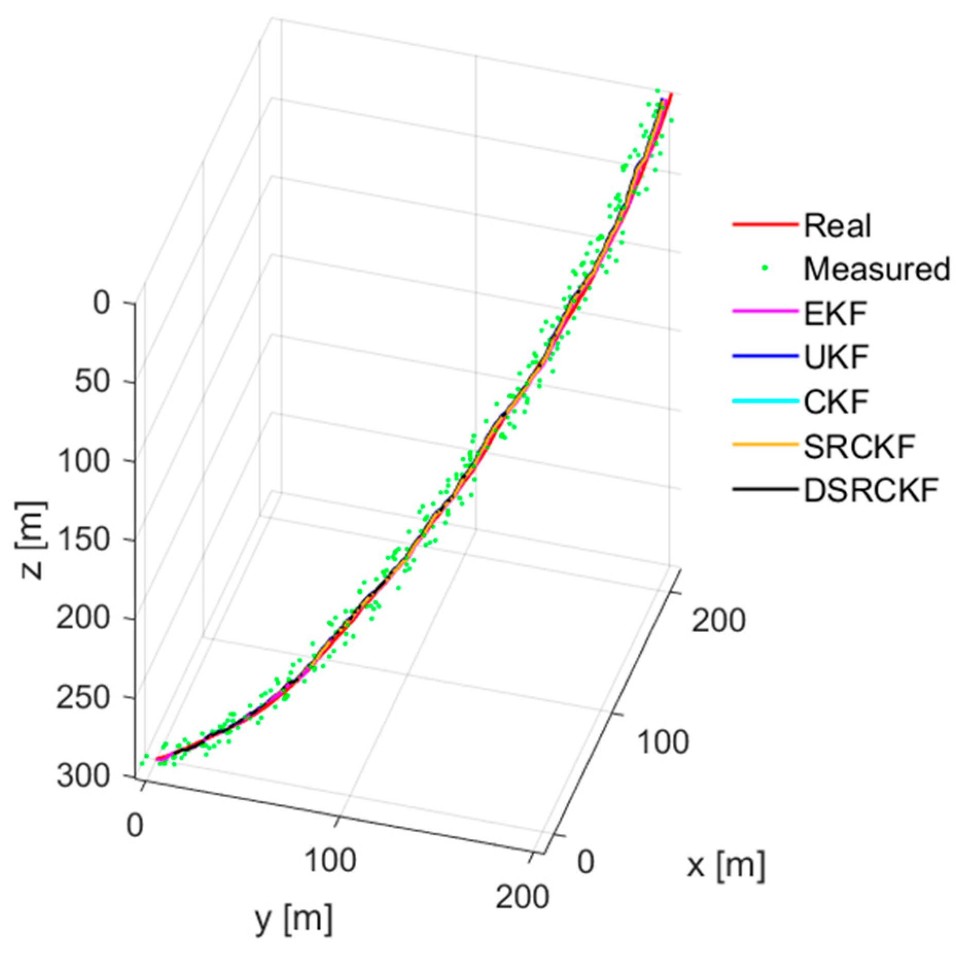
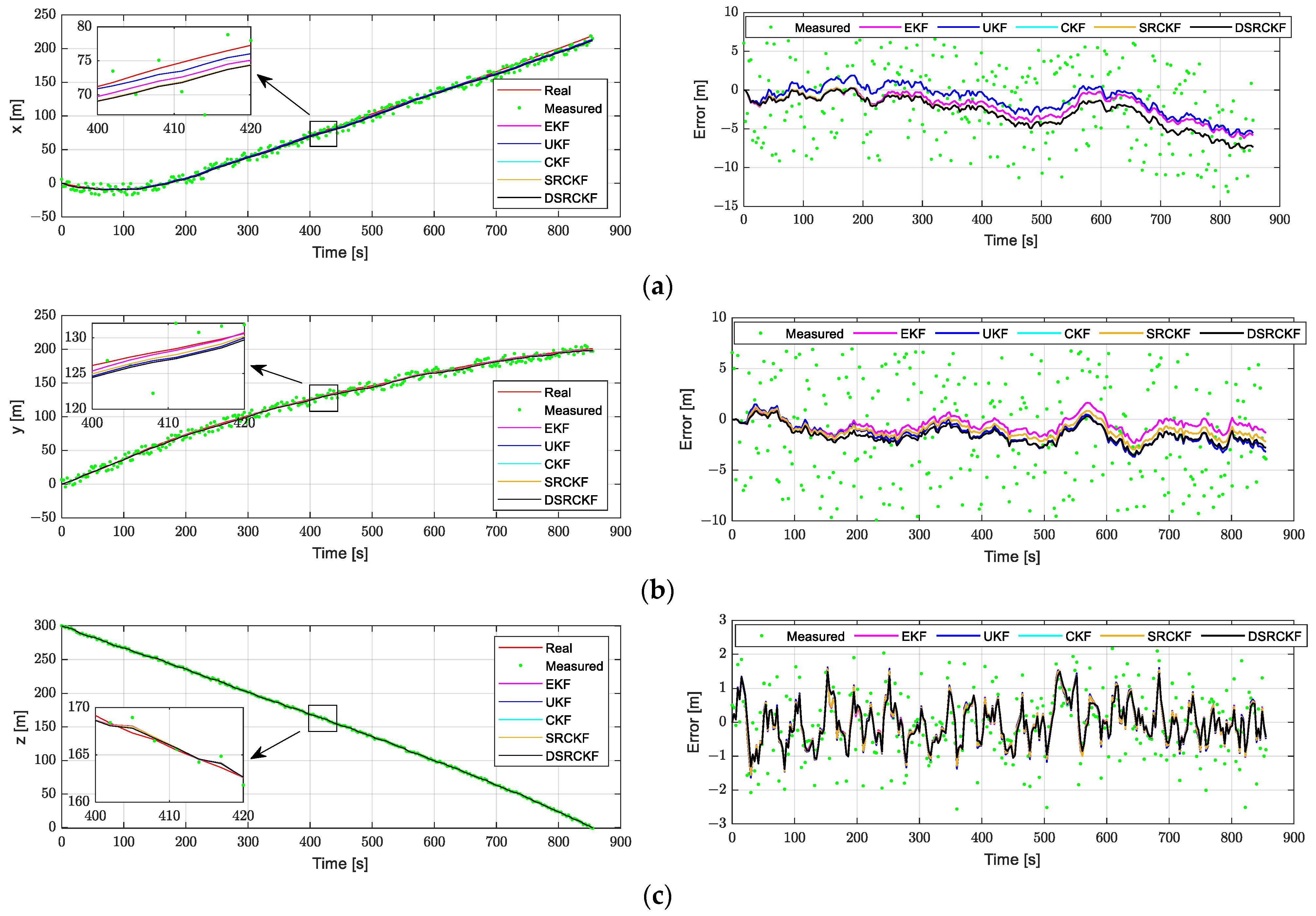
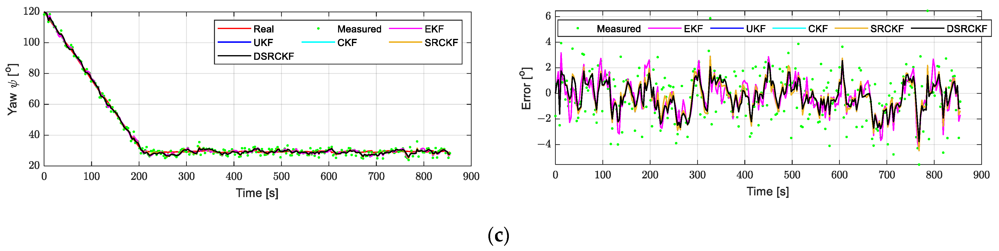
In order to verify the effectiveness of the underwater dead reckoning algorithm for the miniaturized underwater profiler, its underwater navigation performance was tested in a simulation environment. Inertial sensor and depthometer are the two main sensors of a miniaturized underwater profiler. The inertial sensor adopts the mini attitude heading reference system (AHRS) KX-3DM10B, which includes a three-axis Micro Electro Mechanical System (MEMS) gyroscope, three-axis MEMS accelerometer and three-axis magnetoresistive magnetometer. The mini ARHS is small in size, weighs only 18 g, and consumes less than 0.3 W. Its internal update rate is 100 Hz.

Table 2. Performance specifications of mini ARHS KX-3DM10B.

Parameters	Accelerometer	Gyroscope	Magnetometer
Measurement range	$\pm$8 g	$\pm$300°/s	$\pm$1.3 Gs
Bias stability	$\pm$0.003 g	$\pm$0.2°/s	0.01 Gs
Nonlinearity	0.2%	0.2%	0.4%

lists its performance specifications.

The high precision depthometer MS5837 is selected to provide depth information for the miniaturized underwater profiler. The MS5837 is small and lightweight, and weighs only 12 g. Its maximum measurement depth is 300 m, its measurement error is less than 1 m, and the power consumption is less than 0.5 W. All of the relevant error parameters of the sensors are taken as Gaussian noise with a mean value of 0, and their error parameter settings are shown in

Table 3. Error parameter settings for underwater dead reckoning.

Error Parameters	Value
Depthometer	1 m
Attitude angle	2°
Angular velocity	0.2°/s

.

4.2. Simulations

4.2.1. Motion in Fixed Pitch Angle

The miniaturized underwater profiler must adjust the yaw and pitch angles as it floats upward to correct the horizontal offset. A system model is established in MATLAB R2024a software and underwater dead reckoning simulation is conducted. Assuming that the miniaturized underwater profiler performs a gliding and floating motion, the initial floating point of the miniaturized underwater profiler at the depth of the underwater target is selected as the starting point for the underwater dead reckoning process. In the initial stage of floating upward, the miniaturized underwater profiler completes a turning motion with a certain turning radius to reach the desired yaw angle. Then, the miniaturized underwater profiler steadily glides upward at a fixed pitch angle until it reaches the sea surface. The exit point of the miniaturized underwater profiler is taken as the termination point of the underwater navigation process. The position of the starting point is set to a depth of 300 m, with initial yaw angle 120°, desired yaw angle 30°, initial pitch angle 40°, initial axial velocity of 0.5 m/s, and sampling period 3 s.

Set the initial filter values to ${\mathit{\chi }}_0=\left[0;0;300;0;40\pi /180;120\pi /180;0.5;0;0;0;0;0\right]$, $P_0=diag\left(1,1,1,1,1,1,1,1,1,1,1,1\right)$, $R_0=diag\left(1,0.1,0.1,0.1,0.1,0.1,0.1,0.2,0.2,0.2\right)$, $Q_0=diag\left(0.01,0.01,0.001,0.002,0.002,0.002,0.001,0.001,0.0002,0.0002,0.0002,0.0002\right)$, and select a data quality control accuracy $\delta$ of 0.99. According to the chi-square distribution table, it can be found that, when the degree of freedom $n$ is 10, ${\chi }_{\delta ,M}^2$ is 2.558.

Compare the solution results of EKF, UKF, CKF, SRCKF, and DSRCKF algorithms in simulation experiments. As shown in Figure 7, the results obtained when directly using the sensor measurement values have significant errors and EKF, UKF, CKF, SRCKF, and DSRCKF algorithms all have inhibitory effects on measurement errors. Figure 8 shows the displacement and their error plots of the miniaturized underwater profiler in the x, y, and z directions when using EKF, UKF, CKF, SRCKF, and DSRCKF. Figure 9 shows the attitude and their error plots of the miniaturized underwater profiler in the roll, pitch, and yaw.

In order to compare the effectiveness of these algorithms in the underwater dead reckoning of the miniaturized underwater profiler and to eliminate the influence of accidental errors on simulation results, the root mean square error (RMSE) value is used for quantitative analysis. Figure 10 shows position and attitude RMSE values of the miniaturized underwater profiler under 50 times simulations.

In Figure 8, compared with the position error value in the z direction, the position error values in the x and y directions are always larger, and there is no trend of convergence. This is because the data in the x and y directions cannot be directly measured by sensors. Instead, the velocity information in the depth direction and the attitude angle information obtained from the current cycle solution are used to calculate the velocity information in the horizontal direction, and the velocity information is integrated in order to obtain the position information, leading to a certain amount of cumulative error. In the process of underwater dead reckoning (Figure 7, Figure 8, Figure 9 and Figure 10), depth and attitude angle information directly measured by sensors have measurement errors. The measurement error can be significantly reduced through these filtering algorithms, and the values obtained by the DSRCKF algorithm have minimum errors (Figure 10). Therefore, it is demonstrated that the DSRCKF algorithm proposed in this paper has a certain degree of effectiveness.

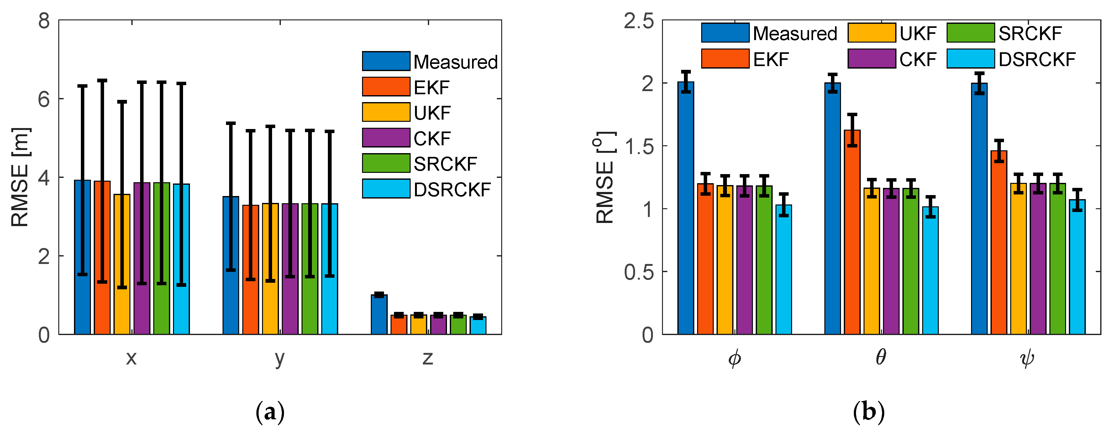
4.2.2. Motion in Different Situations

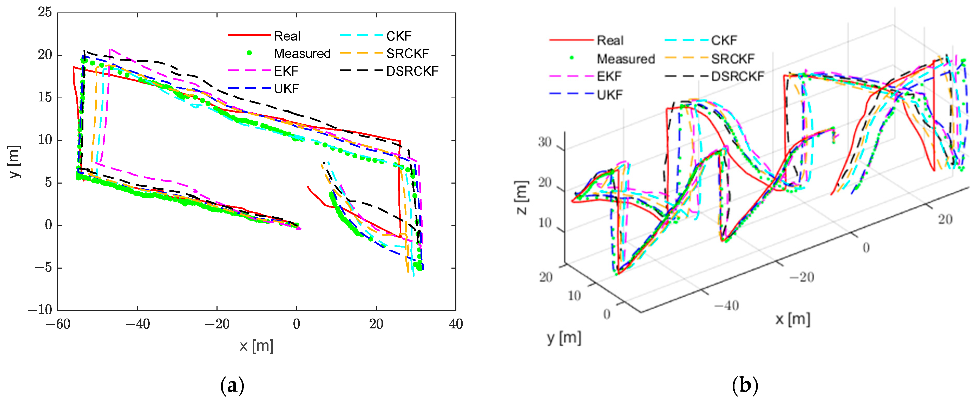
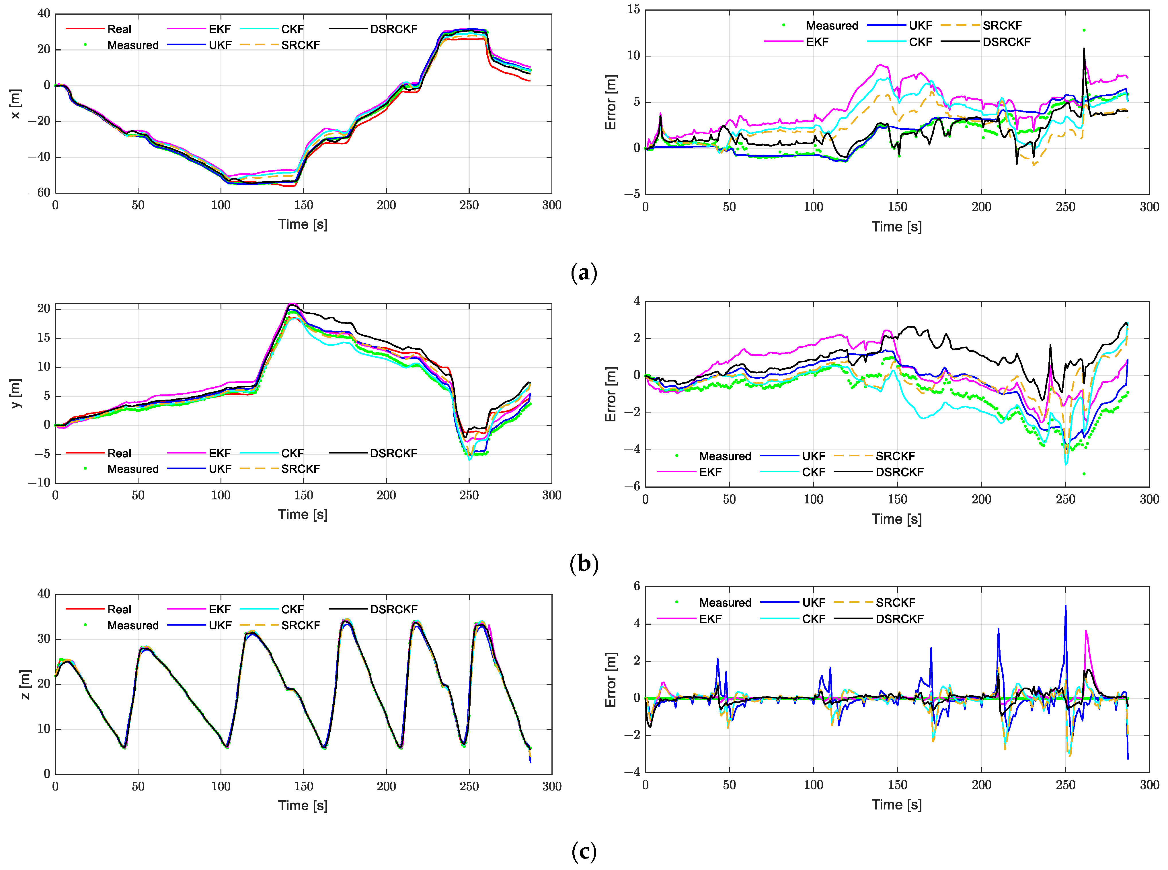
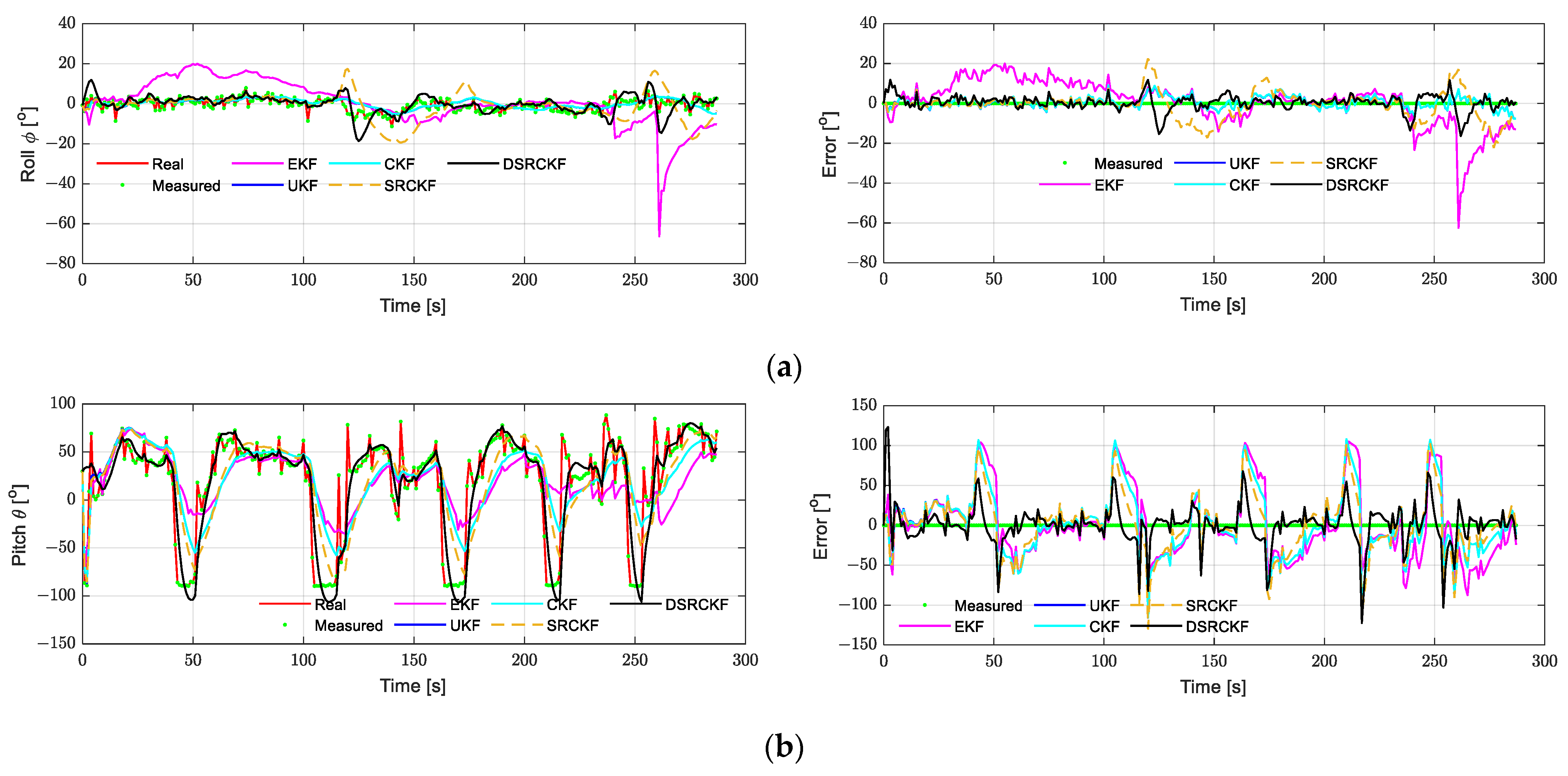
To directly reflect the performance of these navigation algorithm of the miniaturized underwater profiler under various situations, different initial values, such as yaw angles, pitch angles, and axial line velocities of the miniaturized underwater profiler are set. Different initial conditions for dead reckoning simulation are shown in

Table 4. Initial conditions for dead reckoning simulation analysis of the miniaturized underwater profiler.

Parameters	Values
Pitch angle (°)	40, 50, 60
Yaw angle (°)	90, 120, 150
Axial line velocity (m/s)	0.3, 0.4, 0.5, 0.6
Initial depth (m)	300
Desired yaw angle (°)	30

, and corresponding underwater dead reckoning simulation analysis is conducted.

Analyze the RMSE of the pose of the miniaturized underwater profiler in the simulation results to obtain their average values. The position and attitude RMSE values of the miniaturized underwater profiler are shown in Figure 11.

From Figure 11, showing a comprehensive comparison of EKF, UKF, CKF, SRCKF, and DSRCKF for different situations dead reckoning, it can be seen that the RMSE values obtained by using the DSRCKF algorithm in the z direction position and the three-directional attitude angle are smaller than those obtained by other methods. However, the results of those algorithms in the horizontal position (x and y directions) are similar. Therefore, the DSRCKF can provide more reliable underwater pose information for the miniaturized underwater profiler. In order to verify the DSRCKF algorithm, the relevant experimental verification will be conducted in the next section.

4.3. Experiments

Due to the inconvenience of carrying high-precision underwater navigation tracking sensors with large volume and weight for the miniaturized underwater profiler, it is difficult to obtain its real and precise underwater position and attitude. The working principles of drones and underwater profilers are similar in terms of the process of dead reckoning [32,33]. Therefore, this study uses a drone platform to carry the sensors needed for underwater dead reckoning and simulates the movement of the miniaturized underwater profiler while flying in the air. Figure 12 shows the dead reckoning experiment platform, which includes the sensor platform and the drone platform. An RTK device can provide centimeter-level positioning accuracy, so the position information collected by the RTK device can be taken as the real value. AHRS is used to collect the data of the original angle speed, acceleration and geomagnetic strength. The main control module is used to perform attitude angle solution and dead reckoning.

In order to simulate the “diving” and “rising” processes of the miniaturized underwater profiler, the movement of the drone on the horizontal plane is roughly rectangular and the movement of the drone on the vertical plane is sawtooth. The starting point of the drone on the ground is used as the coordinate original point. At the beginning, the drone flew to a certain height, the position is [0, 0, 21.92] m. The measured value of RTK is used as a real trail of the mobile platform and, when combined with AHRS data, the sampling frequency is 1 Hz and the verification of the algorithm of the dead reckoning is performed.

Figure 13 shows the trajectories of the experiment platform obtained by the RTK and the different dead reckoning algorithms. Figure 14 and Figure 15 show the respective position and attitude values and their errors for the experiment platform. The position and attitude RMSE values of the experiment platform are represented in Figure 16. In Figure 16, the data in the x and y directions cannot be obtained directly, the measured value of the horizontal direction of the experiment platform is obtained by combining attitude angle and height data, while other measurements are directly obtained from the sensor. Therefore, the RMSE values for both z direction position and attitude angle of experiment platform are 0.

Combined with Figure 13, Figure 14, Figure 15 and Figure 16, it can be seen that the position values that are directly calculated by the sensor data show the same trend, and that the position errors in the x and y directions are larger than the error in the z direction. According to the position, attitude, and RMSE values, although the DSRCKF algorithm is not optimal in all directions, it can obtain relatively good results, such as in the z direction, pitch angle and yaw angle. This shows that the DSRCKF algorithm proposed in this paper has a certain role in dead reckoning. However, the experiment is based on the verification of the algorithm by drone, and a real underwater test using miniaturized underwater profiler should be carried out in future work. This study does not consider the effect of ocean currents in dead reckoning and wind factors were also not considered during the experiment. Therefore, dead reckoning and designated area persistent monitoring with the miniaturized underwater profiler under the effect of an ocean current should be carried out in subsequent research.

5. Conclusions

Based on the low-cost requirements of ocean designated area persistent monitoring, this paper focuses on the system structure design, dynamic modeling, and underwater dead reckoning algorithm of a miniaturized underwater profiler. The process of designated area persistent monitoring for a miniaturized underwater profiler has been analyzed, and the overall structure of a miniaturized underwater profiler, including barycenter control system and buoyancy regulating system, is designed. Additionally, a dynamic model of the miniaturized underwater profiler is given. The state equation and observation equation of a miniaturized underwater profiler are given. Combining standard SRCKF and adaptive SRCKF, the DSRCKF algorithm is proposed for the dead reckoning of the miniaturized underwater profiler. A comprehensive comparison of EKF, UKF, CKF, SRCKF, and DSRCKF, and of simulations and experiments are conducted. The results show that, compared with the EKF, UKF, CKF, and SRCKF algorithms, the DSRCKF algorithm can improve the accuracy of dead reckoning in the z direction position and attitude angle.

References

1. Lin, M.; Yang, C. Ocean observation technologies: A review. Chin. J. Mech. Eng. 2020, 33, 33–50. [Google Scholar] [CrossRef]
2. Eriksen, C.C.; Osse, T.J.; Light, R.D.; Wen, T.; Lehman, T.W.; Sabin, P.L.; Ballard, J.W.; Chiodi, A.M. Seaglider: A long-range autonomous underwater vehicle for oceanographic research. IEEE J. Ocean. Eng. 2001, 26, 424–436. [Google Scholar] [CrossRef]
3. Webb, D.C.; Simonetti, P.J.; Jones, C.P. Slocum: An underwater glider propelled by environmental energy. IEEE J. Ocean. Eng. 2001, 26, 447–452. [Google Scholar] [CrossRef]
4. Asakawa, K.; Nakamura, M.; Kobayashi, T.; Watanabe, Y.; Hyakudome, T.; Ito, Y.; Kojima, J. Design concept of Tsukuyomi—Underwater glider prototype for virtual mooring. In Proceedings of the OCEANS 2011 IEEE—Spain, Santander, Spain, 6–9 June 2011; pp. 1–5. [Google Scholar] [CrossRef]
5. Huang, Y.-W.; Ueda, K.; Itoh, K.; Sasaki, Y.; Debenest, P.; Fukushima, E.F.; Hirose, S. Development of tether mooring type underwater robots: Anchor diver I and II. Indian J. Mar. Sci. 2011, 40, 181–190. [Google Scholar]
6. Rainville, L.; Pinkel, R. Wirewalker: An autonomous wave-powered vertical profiler. J. Atmos. Ocean. Technol. 2001, 18, 1048–1051. [Google Scholar] [CrossRef]
7. Ten Doeschate, A.; Sutherland, G.; Esters, L.; Wain, D.; Walesby, K.; Ward, B. ASIP: Profiling the upper ocean. Oceanography 2017, 30, 33–35. [Google Scholar] [CrossRef]
8. Toole, J.M.; Krishfield, R.A.; Timmermans, M.-L.; Proshutinsky, A. The ice-tethered profiler: Argo of the arctic. Oceanography 2011, 24, 126–135. [Google Scholar] [CrossRef]
9. Andre, X.; Reste, S.L.; Rolin, J.-F. Arvor-c: A coastal autonomous profiling float. Sea Technol. 2010, 51, 10–13. [Google Scholar]
10. Zhou, P.; Yang, C.; Wu, S.; Zhu, Y. Designated area persistent monitoring strategies for hybrid underwater profilers. IEEE J. Ocean. Eng. 2020, 45, 1322–1336. [Google Scholar] [CrossRef]
11. Yang, C.; Wu, D.; Zhou, P.; Ma, S.; Zhou, R.; Zhang, X.; Zhang, Y.; Xia, Q.; Wu, Z. Research on ocean-current-prediction-based virtual mooring strategy for the portable underwater profilers. Appl. Ocean Res. 2024, 142, 103810. [Google Scholar] [CrossRef]
12. Kemp, B.; Janssen, A.J.M.W.; van der Kamp, B. Body position can be monitored in 3D using miniature accelerometers and earth-magnetic field sensors. Electroencephalogr. Clin. Neurophysiol. 1998, 109, 484–488. [Google Scholar] [CrossRef] [PubMed]
13. Liu, J.; Yu, T.; Wu, C.; Zhou, C.; Lu, D.; Zeng, Q. A low-cost and high-precision underwater integrated navigation system. J. Mar. Sci. Eng. 2024, 12, 200. [Google Scholar] [CrossRef]
14. Xu, B.; Hu, J.; Guo, Y. An acoustic ranging measurement aided SINS/DVL integrated navigation algorithm based on multivehicle cooperative correction. IEEE Trans. Instrum. Meas. 2022, 71, 8504615. [Google Scholar] [CrossRef]
15. Fukuda, G.; Kubo, N. Application of initial bias estimation method for inertial navigation system (INS)/Doppler velocity log (DVL) and INS/DVL/gyrocompass using micro-electro-mechanical system sensors. Sensors 2022, 22, 5334. [Google Scholar] [CrossRef] [PubMed]
16. Ghanipoor, F.; Alasty, A.; Salarieh, H.; Hashemi, M.; Shahbazi, M. Model identification of a marine robot in presence of IMU-DVL misalignment using TUKF. Ocean Eng. 2020, 206, 107344. [Google Scholar] [CrossRef]
17. Karmozdi, A.; Hashemi, M.; Salarieh, H. Design and practical implementation of kinematic constraints in inertial navigation system-Doppler velocity log (IND-DVL)-based navigation. Navigation 2018, 65, 629–642. [Google Scholar] [CrossRef]
18. Tal, A.; Klein, I.; Katz, R. Inertial navigation system/Doppler velocity log (INS/DVL) fusion with partial DVL measurements. Sensors 2017, 17, 415. [Google Scholar] [CrossRef] [PubMed]
19. Gao, W.; Zhang, Y.; Wang, J. A strapdown interial navigation system/beidou/doppler velocity log integrated navigation algorithm based on a cubature Kalman filter. Sensors 2014, 14, 1511–1527. [Google Scholar] [CrossRef] [PubMed]
20. Huang, H.; Chen, X.; Zhou, Z.; Xu, Y.; Lv, C. Study of the algorithm of backtracking decoupling and adaptive extended Kalman filter based on the quaternion expanded to the state variable for underwater glider navigation. Sensors 2014, 14, 23041–23066. [Google Scholar] [CrossRef] [PubMed]
21. Allotta, B.; Pugi, L.; Bartolini, F.; Ridolfi, A.; Costanzi, R.; Monni, N.; Gelli, J. Preliminary design and fast prototyping of an autonomous underwater vehicle propulsion system. Proc. Inst. Mech. Eng. M J. Eng. 2014, 229, 248–272. [Google Scholar] [CrossRef]
22. Allotta, B.; Caiti, A.; Costanzi, R.; Fanelli, F.; Fenucci, D.; Meli, E.; Ridolfi, A. A new AUV navigation system exploiting unscented Kalman filter. Ocean Eng. 2016, 113, 121–132. [Google Scholar] [CrossRef]
23. Garcia, R.V.; Pardal, P.C.P.M.; Kuga, H.K.; Zanardi, M.C. Nonlinear filtering for sequential spacecraft attitude estimation with real data: Cubature Kalman filter, unscented Kalman filter and extended Kalman filter. Adv. Space Res. 2019, 63, 1038–1050. [Google Scholar] [CrossRef]
24. Davari, N.; Gholami, A. An asynchronous adaptive direct Kalman filter algorithm to improve underwater navigation system performance. IEEE Sens. J. 2017, 17, 1061–1068. [Google Scholar] [CrossRef]
25. Emami, M.; Taban, M.R. A customized h-infinity algorithm for underwater navigation system: With experimental evaluation. Ocean Eng. 2017, 130, 611–619. [Google Scholar] [CrossRef]
26. Huang, H.; Chen, X.; Zhou, Z.; Lv, C. Attitude determination for underwater gliders using unscented Kalman filter based on smooth variable algorithm. J. Coast. Res. 2015, 73, 698–704. [Google Scholar] [CrossRef]
27. Huang, H.; Chen, X.; Zhang, B.; Wang, J. High accuracy navigation information estimation for inertial system using the multi-model EKF fusing adams explicit formula applied to underwater gliders. ISA Trans. 2017, 66, 414–424. [Google Scholar] [CrossRef]
28. Zhang, Y.; Ding, B.; Huang, X.; Yang, T.; Liu, X. Multi-sensor, adjustable-period integrated navigation method based on multi-stage signal trigger for underwater vehicles. J. Navig. 2017, 71, 208–220. [Google Scholar] [CrossRef]
29. Arasaratnam, I.; Haykin, S. Cubature Kalman filters. IEEE Trans. Autom. Control 2009, 54, 1254–1269. [Google Scholar] [CrossRef]
30. Arasaratnam, I.; Haykin, S.; Hurd, T.R. Cubature Kalman filtering for continuous-discrete systems: Theory and simulations. IEEE Trans. Signal Process. 2010, 58, 4977–4993. [Google Scholar] [CrossRef]
31. Huang, H.; Shi, R.; Zhou, J.; Yang, Y.; Song, R.; Chen, J.; Wu, G.; Zhang, J. Attitude determination method integrating square-root cubature Kalman filter with expectation-maximization for inertial navigation system applied to underwater glider. Rev. Sci. Instrum. 2019, 90, 095001. [Google Scholar] [CrossRef] [PubMed]
32. Li, L.; Wang, S.; Zhang, Y.; Song, S.; Wang, C.; Tan, S.; Zhao, W.; Wang, G.; Sun, W.; Yang, F.; et al. Aerial-aquatic robots capable of crossing the air-water boundary and hitchhiking on surfaces. Sci. Robot. 2022, 7, eabm6695. [Google Scholar] [CrossRef] [PubMed]
33. Bai, Y.; Jin, Y.; Liu, C.; Zeng, Z.; Lian, L. Nezha-f: Design and analysis of a foldable and self-deployable HAUV. IEEE Robot. Autom. Lett. 2023, 8, 2309–2316. [Google Scholar] [CrossRef]
Figure 1. Schematic diagram of the designated area persistent monitoring process of the miniaturized underwater profiler.
Jmse 12 01146 g001
Figure 2. Diagram of the entire structure of the miniaturized underwater profiler: (a) schematic diagram and (b) physical structure.
Jmse 12 01146 g002
Figure 3. Dual mass block barycenter control system of the miniaturized underwater profiler: (a) schematic diagram, (b) real product, and (c) the relationships between the position of dual mass block and the attitude of the profiler.
Jmse 12 01146 g003
Figure 4. Buoyancy regulating system for the miniaturized underwater profiler: (a) schematic diagram and (b) the real product.
Jmse 12 01146 g004
Figure 5. Definition of the coordinate system of the miniaturized underwater profiler.
Jmse 12 01146 g005
Figure 6. The filter structure of the underwater dead reckoning sensor system for the miniaturized underwater profiler.
Jmse 12 01146 g006
Figure 7. Motion trajectory diagram of the miniaturized underwater profiler in simulation.
Jmse 12 01146 g007
Figure 8. The position and error values of the miniaturized underwater profiler: (a) the position and error values in the x direction, (b) the position and error values in the y direction, and (c) the position and error values in the z direction.
Jmse 12 01146 g008
Figure 9. The attitude and error values of the miniaturized underwater profiler: (a) the attitude and error values in roll, (b) the attitude and error values in pitch, and (c) the attitude and error values in yaw.
Jmse 12 01146 g009aJmse 12 01146 g009b
Figure 10. The position and attitude RMSE values of the miniaturized underwater profiler in fixed pitch angle: (a) position and (b) attitude.
Jmse 12 01146 g010
Figure 11. The position and attitude RMSE values of the miniaturized underwater profiler in different situations: (a) position and (b) attitude.
Jmse 12 01146 g011
Figure 12. Experiment platform, including sensor platform and drone platform.
Jmse 12 01146 g012
Figure 13. Comparison of the real and the calculated trajectory of the experiment platform: (a) 2D and (b) 3D.
Jmse 12 01146 g013
Figure 14. The position and error values of the experiment platform: (a) the position and error values in the x direction, (b) the position and error values in the y direction, and (c) the position and error values in the z direction.
Jmse 12 01146 g014
Figure 15. The attitude and error values of the experiment platform: (a) the attitude and error values in roll, (b) the attitude and error values in pitch and (c) the attitude and error values in yaw.
Jmse 12 01146 g015aJmse 12 01146 g015b
Figure 16. The position and attitude RMSE values of the experiment platform: (a) position and (b) attitude.
Jmse 12 01146 g016