Construction of a Real-Time Forecast Model with Deep Learning Techniques for Coastal Engineering and Processes: Nested in a Basin Scale Suite of Models

Abstract

This study aims to develop a robust and adaptable real-time forecasting system for coastal and estuarine regions, considering the challenges posed by the limited or unavailable forecast data. A real-time forecast system has been designed to handle three distinct scenarios: forecast data from global models are available, unavailable, or intermittently unavailable. To address the challenge of data unavailability, this research proposes the application of a deep learning model (DLM). This study involves the construction of a high-resolution numerical model nested within global models. The performance of the DLM is evaluated by comparing the simulation results of the nested model generated using DLM-predicted data against those obtained using data from global models. The results demonstrate a high correlation and around 90% accuracy for up to the initial 5 days of the forecast. Even in the absence of hindcast data up to 4 days prior to the forecast beginning time, the real-time forecast with DLM can achieve an accuracy exceeding 70% of the forecast data from global models. However, direct application of the developed DLM to an unknown domain results in significantly lower performance, highlighting the importance of retraining the DLM with local data. Overall, this study presents a comprehensive approach to constructing a real-time forecasting system for coastal and estuarine regions that adeptly handles various data availability scenarios through the integration of machine learning techniques.

1. Introduction

Numerical simulations of estuarine and coastal hydrodynamics provide a detailed and quantitative understanding of essential hydrodynamic processes, serving as an effective tool to predict water movement and the spatial and temporal variations of key water properties. This is crucial for marine system studies, including water quality and ecosystem dynamics. Consequently, numerical simulations, combined with measured data, deliver thorough insights into estuarine dynamics. Hydrodynamic modeling underpins the study of morphology, waves, sediment transport, and water quality. The main factors influencing hydrodynamics in shallow estuarine or coastal areas are tides, sea level changes, river inflows, waves, storm surges, and meteorological forces.

High-resolution coastal models are now extensively utilized as tools for coastal management. Coastal ocean conditions, such as the sea level fluctuations along the East Coast, are also affected by large-scale processes like the Gulf Stream [1]. Global models, with their coarse resolution, are inadequate for capturing phenomena that require finer spatial resolution, such as oil spills and tidal inlet flows. Downscaling from global models can help better resolve regional and local features compared to lower-resolution models. Therefore, nesting and downscaling global models onto high-resolution coastal models can be an effective approach for accurately capturing coastal hydrodynamics. Nesting coastal models with basin-scale models, along with the assimilation of observational data, enhances model performance across all scales [2,3]. Developing structured grid models and nesting them within large-scale models is a practical solution for addressing the wide range of spatial and temporal motion scales [4,5,6,7]. This approach involves transferring data from the coarse global model to the higher resolution model focusing on a specific smaller area.

Assigning open boundary conditions to coastal models is crucial because these boundary conditions significantly impact the accuracy of the results. Coastal circulation has unique dynamics compared to the deep ocean, influenced by factors such as shallowness, strong tidal effects, proximity to the coast, flow convergence and divergence due to coastal features, stratification, and river inflows. In coastal areas, bottom-drag forces and tidal effects are more pronounced than in the deep ocean [8]. To reduce computational costs, model areas can be confined to a specific scale based on the area of interest. Open boundary conditions are used to represent the influence of areas outside the model domain that are not explicitly modeled.

Machine learning has gained significant traction as a research method in numerous fields, including wave modeling, ocean data analysis, weather prediction, climate modeling, and marine environments [9,10,11,12]. The application of deep learning was explored, specifically convolutional neural networks (CNNs), for simulating ocean currents in a study [13]. The study aimed to investigate whether CNNs could capture the spatial–temporal variability of eddy momentum forcing, respect global momentum conservation, predict sub-surface flow fields, and be sensitive to physical processes. The study demonstrated that CNNs can effectively represent the spatial–temporal variability of eddy momentum forcing using data from idealized high-resolution ocean models, neural networks can be constrained to respect momentum conservation without significant loss of accuracy and accurately predict sub-surface flow fields.

The forecasting model is particularly valuable for predicting hydrodynamic conditions in study areas, which can affect dredging projects and other engineering tasks. Additionally, when integrated with the water quality model, it serves as a foundation for continuous environmental assessments. To set up the forecast model, an automated system needs to be developed and forecast boundary conditions data are required, which may not always be available. Deep or machine learning techniques are one approach that can resolve this issue of data unavailability. A deep learning model (DLM) can be applied to create boundary condition data projected into the future using archived data. This data-driven method can be applied anywhere where there is limited or no forecast data available. The complexity of the machine learning model arises when outputs are not only dependent on inputs at the current point in time but also previous points in time, which requires deep learning approaches due to its capabilities to recognize patterns in time series data. CNN methods have time series pattern recognition capacity. A hybrid approach can be developed combining DLM and global models to construct a robust and adaptable forecast system.

2. Methods

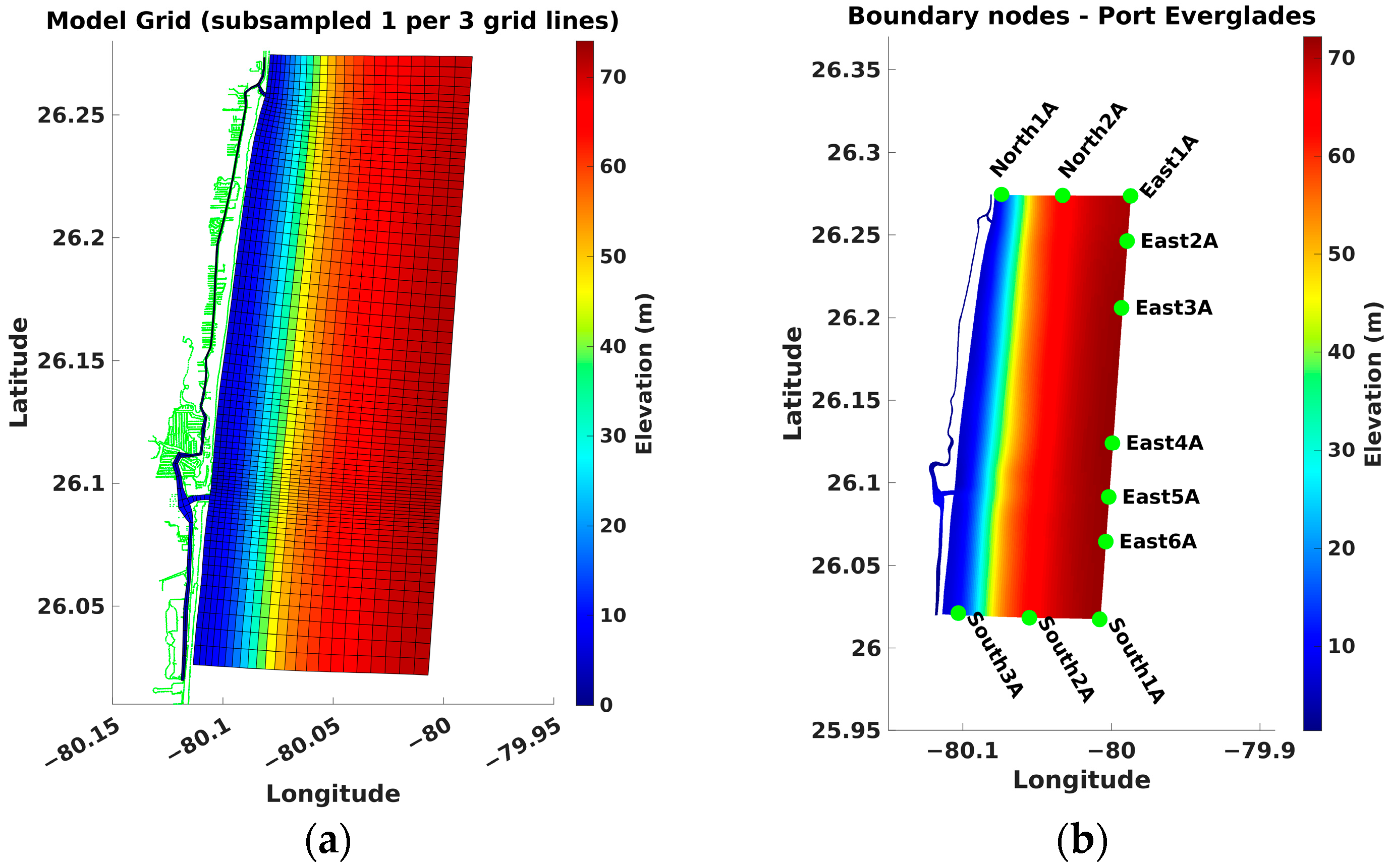
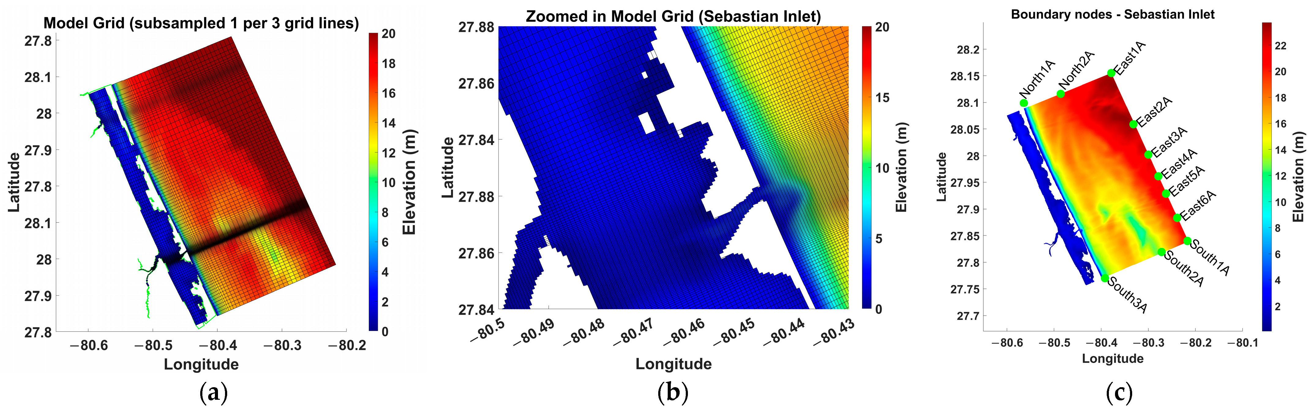
2.1. Model Grid

Numerical models were developed for the central IRL (Figure 1). The description of the study area can be found in [14]. The physical model was developed utilizing Delft3D, which is an open-source, 3D, finite difference-based modeling system [15]. The model employed a curvilinear orthogonal computational grid, with grid size varying from 14 m in the river and inlets to 475 m in the coastal area (Figure 2) and was composed of five sigma layers. The grid represents the intricate coastline, particularly focusing on the Sebastian Inlet. This grid represents the coastline from Wabasso Beach to Indialantic Beach (Figure 1).

2.2. Model Setup

This model’s configuration can be found in [14]. The description of bathymetric data collection, vertical layer distribution, bottom roughness setup, flow, and transport boundary conditions can be found in the study [14]. A description of the model’s performance and skills can be found in [14]. Topographic data were collected from NOAA [17], surface elevation, water temperature, and salinity were obtained from HYCOM [18], and meteorological forcings were retrieved from NARR [19]. Model adjustments and calibration followed similar methods described in [20].

3. Machine Learning Techniques

DLMs were developed for the Sebastian Inlet model using CNNs to acquire boundary conditions data, including water level, salinity, and water temperature for a real-time forecast model. Initially, patterns of dependence in the time series of these parameters were explored. Time series exhibit three patterns of dependence—trend, seasonality, and cyclic behavior. Trends in a time series reveal consistent, long-term patterns over an extended period, representing the series’ longest time-scale changes. Seasonality in a time series indicates periodic changes, occurring at specific time frequencies such as daily, weekly, monthly, or yearly repetitions. Following the examination of time series patterns, they are employed in CNN for multi-step predictions. Detailed methods for developing and validating DLMs are outlined in the following sections.

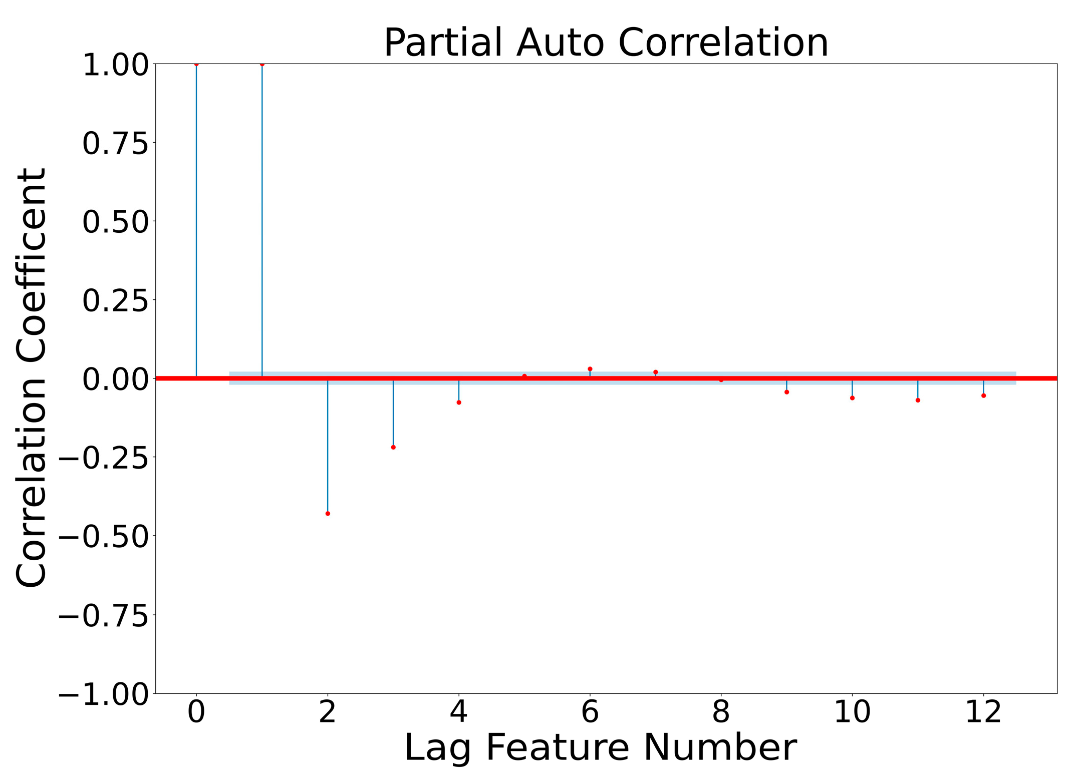
3.1. Lag Plot

To assess the serial dependence of a time series, a lagged time series can be derived by shifting the values of the original time series forward or backward by one or multiple timesteps.

Table 1. Time series of lag features for 1–12 hourly time steps. NAN (not a number) illustrates shifted time series.

Salinity	Lag 1	Lag 2	Lag 3	Lag 4	Lag 5	Lag 6	Lag 7	Lag 8	Lag 9	Lag 10	Lag 11	Lag 12
36.309	NaN	NaN	NaN	NaN	NaN	NaN	NaN	NaN	NaN	NaN	NaN	NaN
36.324	36.309	NaN	NaN	NaN	NaN	NaN	NaN	NaN	NaN	NaN	NaN	NaN
36.346	36.324	36.309	NaN	NaN	NaN	NaN	NaN	NaN	NaN	NaN	NaN	NaN
36.369	36.346	36.324	36.309	NaN	NaN	NaN	NaN	NaN	NaN	NaN	NaN	NaN
36.389	36.369	36.346	36.324	36.309	NaN	NaN	NaN	NaN	NaN	NaN	NaN	NaN
36.404	36.389	36.369	36.346	36.324	36.309	NaN	NaN	NaN	NaN	NaN	NaN	NaN
36.414	36.404	36.389	36.369	36.346	36.324	36.309	NaN	NaN	NaN	NaN	NaN	NaN
36.418	36.414	36.404	36.389	36.369	36.346	36.324	36.309	NaN	NaN	NaN	NaN	NaN
36.417	36.418	36.414	36.404	36.389	36.369	36.346	36.324	36.309	NaN	NaN	NaN	NaN
36.414	36.417	36.418	36.414	36.404	36.389	36.369	36.346	36.324	36.309	NaN	NaN	NaN
36.408	36.414	36.417	36.418	36.414	36.404	36.389	36.369	36.346	36.324	36.309	NaN	NaN
36.403	36.408	36.414	36.417	36.418	36.414	36.404	36.389	36.369	36.346	36.324	36.309	NaN
36.398	36.403	36.408	36.414	36.417	36.418	36.414	36.404	36.389	36.369	36.346	36.324	36.309
36.397	36.398	36.403	36.408	36.414	36.417	36.418	36.414	36.404	36.389	36.369	36.346	36.324

illustrates this concept, where the salinity data are shifted 12 steps forward with a time interval of 1 h. This operation allows for the creation of lagged time series that capture the serial dependencies of the values within the original time series. By examining the relationships between the original time series and its lagged counterparts, insights into the temporal dependencies and patterns can be gained.

Partial autocorrelation analysis provides insights into the correlation between a time series and its lagged time series, aiding in the identification of suitable lag features. In Figure 3, the partial autocorrelation plot reveals that lags 1 and 2 fall outside the range of no correlation (indicated by the shaded red zone) and exhibit a higher correlation compared to other lag features. This finding suggests that using lag 1–2 as lag features would be appropriate for predicting salinity data up to two steps forward in time.

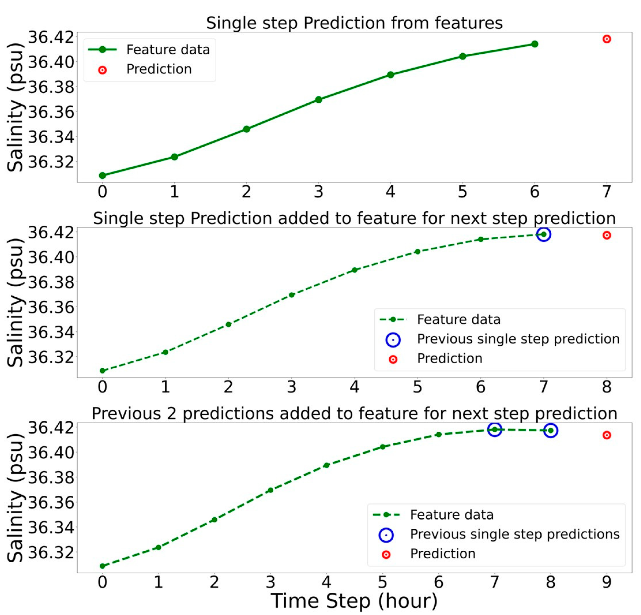
3.2. Multi-Step Predictions

In the previous section, the DLM was utilized to predict a two-time-step (2-hourly steps) forecast based on the strong correlation observed up to two lag features in the partial autocorrelation analysis. However, real-world applications often require multi-step predictions. In this study, a forecast spanning 7 days, equivalent to 168 timesteps at an hourly interval, was desired. Consequently, a suitable approach needed to be developed to achieve multi-step prediction.

There are various methods available for multi-step forecasting, including multioutput, direct, recursive, and hybrid methods. In the multioutput strategy, all outputs for the forecast horizon are predicted simultaneously in one step. This approach is straightforward and efficient for short-term predictions but tends to introduce more errors over longer forecast periods. On the other hand, the direct strategy involves developing separate DLMs for each forecast step: one model predicts one step ahead, another predicts two steps ahead, and so forth. For instance, forecasting 7 days requires developing 168 individual DLMs, making it computationally intensive. A hybrid approach combines elements of both recursive and direct methods. The hybrid method was not selected in this study due to its complexity, computational expense, and the propagation errors associated with it.

In this study, a recursive strategy was adopted to obtain the desired seven-day forecast. The recursive method involves iteratively generating one-step predictions and incorporating them back into the model for subsequent predictions, thus extending the forecast horizon to the desired length. By repeating this process, a multi-step forecast spanning the desired period can be achieved.

However, in the recursive strategy, there is a possibility of error propagation throughout the forecast horizon. As the forecast progresses further in time, the errors from previous predictions may accumulate, potentially leading to increased errors as the forecast extends. Figure 4 illustrates the recursive prediction strategy using the example of salinity forecasting.

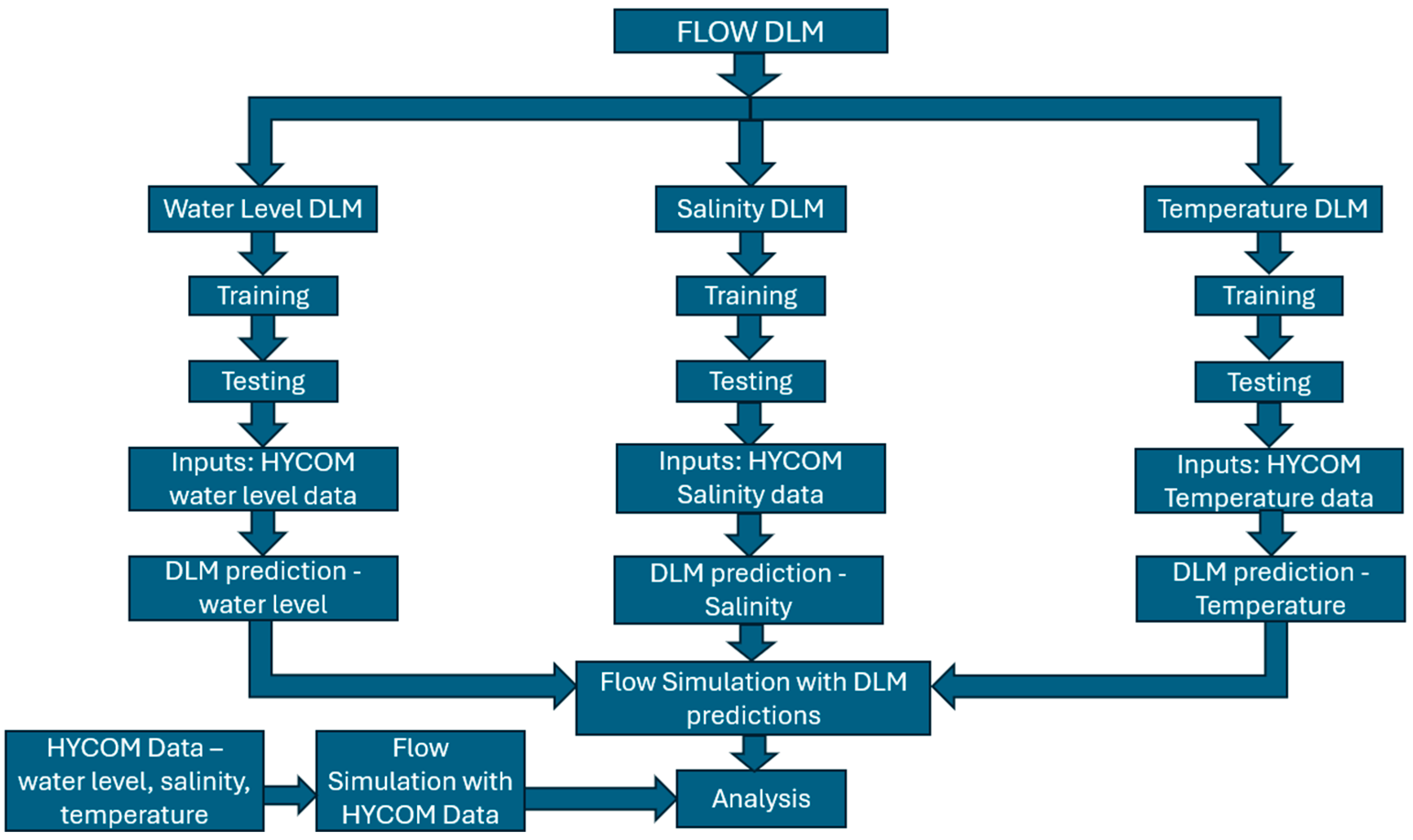
3.3. Workflow

The Flow DLM is a set of salinity, water temperature, and water level DLM. Each DLM was trained with HYCOM data near the Sebastian Inlet region. Water level, salinity, and water temperature DLMs were trained with HYCOM water level, salinity, and water temperature data, respectively. Each DLM was trained and tested with two separate datasets. Trained and tested DLMs were used to predict forecast data for boundary forcings for flow simulations.

The DLM developed here is not a surrogate or substitute for a physics-based model. The primary objective of this study is to generate real-time forecast data in scenarios where such data are unavailable from global models. The forecast data from the DLM will serve as boundary conditions for simulations conducted using the physics-based model (Delft3D). Integrating the DLM with all three parameters into one model would increase complexity compared to the current approach of developing separate DLMs for each parameter.

Prior to the application of this DLM for real-time forecasting, it is imperative to test and analyze it with Delft3D simulations. Two separate simulations were undertaken: one employing data from global models and the other utilizing data predicted by the DLM. The results derived from these simulations were then statistically evaluated at predefined observation stations. The analysis of these simulation results aids in determining the accuracy of the DLM-predicted boundary conditions in reproducing hydrodynamics. If the simulation results, using DLM-predicted data, exhibit strong correlations with the results from the simulation using data from global models, it can be inferred that the DLM method could be employed in scenarios where forecasts from global models are not readily available. Figure 5 illustrates the flowchart for Flow DLM.

3.4. Train–Test Data

Before applying the DLM, the data underwent preprocessing steps. Initially, the dataset was divided into two subsets: a training set comprising 80% of the data and a test set containing the remaining 20%. The DLM was developed using the training data and subsequently tested using the test data, which was separate from the training domain. This test dataset provided an unbiased evaluation of the model’s performance. In this study, three years of HYCOM data spanning from 2018 to 2020 were prepared. The model was trained using data from January 2018 to April 2020, whereas the remainder of these data from May 2020 to December 2020 were utilized for testing. The DLM approach was employed for both the training and test datasets, enabling the prediction of two forward time steps. Training, testing, inputs, and DLM predictions are conducted for all 11 boundary nodes (see Figure 2c). However, all the figures presented in the following sections are specifically for the East1A boundary nodes only (see Figure 2c), and additional figures for another node (south1A) are presented in Appendix A (Figure A5 and Figure A6).

The water level DLM was specifically trained using water level data from HYCOM, covering the period from January 2018 to April 2020. Figure 6a presents the DLM’s predicted training data, demonstrating a strong correlation coefficient of 0.98 between the predicted water level values and the actual training data (Figure 6b). This high correlation indicates that the water level DLM model can effectively capture and replicate the patterns and variations in the training data.

The DLM-predicted test data for the water level in Figure 7a demonstrate excellent agreement in terms of capturing the phase, indicating that the water level variations are accurately predicted. However, there is a slight discrepancy in capturing the lowest point in the amplitude, suggesting that the model may have underestimated the minimum and maximum water level. Nevertheless, the margin of error for the amplitudes is relatively small, indicating a high level of accuracy in predicting the water level variations. In the correlation plot (Figure 7b), all the data points are closely aligned around the center line, indicating a strong correlation (correlation coefficient of 0.98) between the predicted and observed water levels. In a similar manner, salinity and water temperature DLMs were developed (see Appendix A).

3.5. DLM Inputs and Predictions

For the flow DLM, the input length was set to 144 hindcast time steps. If the available hindcast dataset was provided at an hourly resolution, then the DLM required 6 days’ worth of hindcast data. The specific length of 144 time steps was determined during the model training phase, as it yielded better results. However, the length could be adjusted if desired during training. In this study, a 7-day prediction was conducted using a random period of 12 February 2021 to 19 February 2021. The input data for this prediction consisted of hindcast data from 6 February 2021 to 12 February 2021. Two separate simulations were performed: one using the predicted data from the DLM and another using the corresponding HYCOM data from the same period. To evaluate the accuracy of the DLM predictions, the results from these two simulations were compared and analyzed. By examining the agreement between the DLM predictions and the HYCOM data, the performance and reliability of the DLM for flow simulations can be assessed.

The provided water level data spanned from 6 February 2021 to 12 February 2021, and a seven-day forecast was generated from 12 February 2021 to 19 February 2021 (Figure 8). This seven-day forecast was used for flow simulation in Section 3.6.

The provided salinity inputs spanned from 6 February 2021 to 12 February 2021, and a seven-day forecast had been generated from 12 February 2021 to 19 February 2021. The salinity inputs were provided for each of the five layers into salinity DLM (Figure 9a), and the prediction was conducted separately for each layer (Figure 9b). The seven-day forecast provided predictions of salinity values for each layer from 12 February 2021 to 19 February 2021.

Using water temperature data from 6 February 2021 to 12 February 2021 as inputs, a seven-day forecast from 12 February 2021 to 19 February 2021 was generated using the trained water temperature DLM. Inputs were provided for each of the 5 layers (Figure 10a), allowing for predictions to be conducted separately for each layer (Figure 10b).

3.6. Flow Simulations

To evaluate the performance of the DLM prediction, separate simulations were conducted using the DLM-predicted data and HYCOM data for the same period. The objective is to compare the results from these simulations and assess how accurately the simulation with DLM predictions replicates the simulation with HYCOM data.

In the first simulation, boundary forcing files were created using the DLM-predicted water level time series (blue line in Figure 11), salinity profiles (Figure 12a), and water temperature profiles (Figure 13a) for the period of 12 February 2021 to 19 February 2021. These boundary conditions were used to drive the first Delft3D flow simulation.

In the second simulation, boundary forcing files were created using the water level time series (red line in Figure 11), salinity profiles (Figure 12b), and water temperature profiles (Figure 13b) obtained from HYCOM data for the same time window. These HYCOM-based boundary conditions were used to drive the second Delft3D flow simulation.

By comparing the results from these two simulations, this study aims to assess how accurately the DLM-predicted data replicates the simulation results obtained from the HYCOM data. A comparative analysis will provide insights into the accuracy and reliability of the DLM predictions and their suitability for driving the Delft3D flow simulation. It will help assess the performance of the DLM in generating reliable boundary conditions and its potential for improving real-time forecasting capabilities in the study area.

4. Results

The results from the two flow simulations, one using DLM-predicted boundary conditions (first simulation) and the other using boundary conditions derived from HYCOM data (second simulation), were compared at three stations: North Jetty, inside Sebastian Inlet, and the LOBO station inside the IRL estuary (see location in Figure 1b). The comparison involved analyzing the time series of model results for water level, salinity, water temperature, and the u and v components of velocity. At each station, the time series of model results for the various parameters were obtained for both the first and second simulations. These time series were then compared to assess the agreement or differences between the simulations.

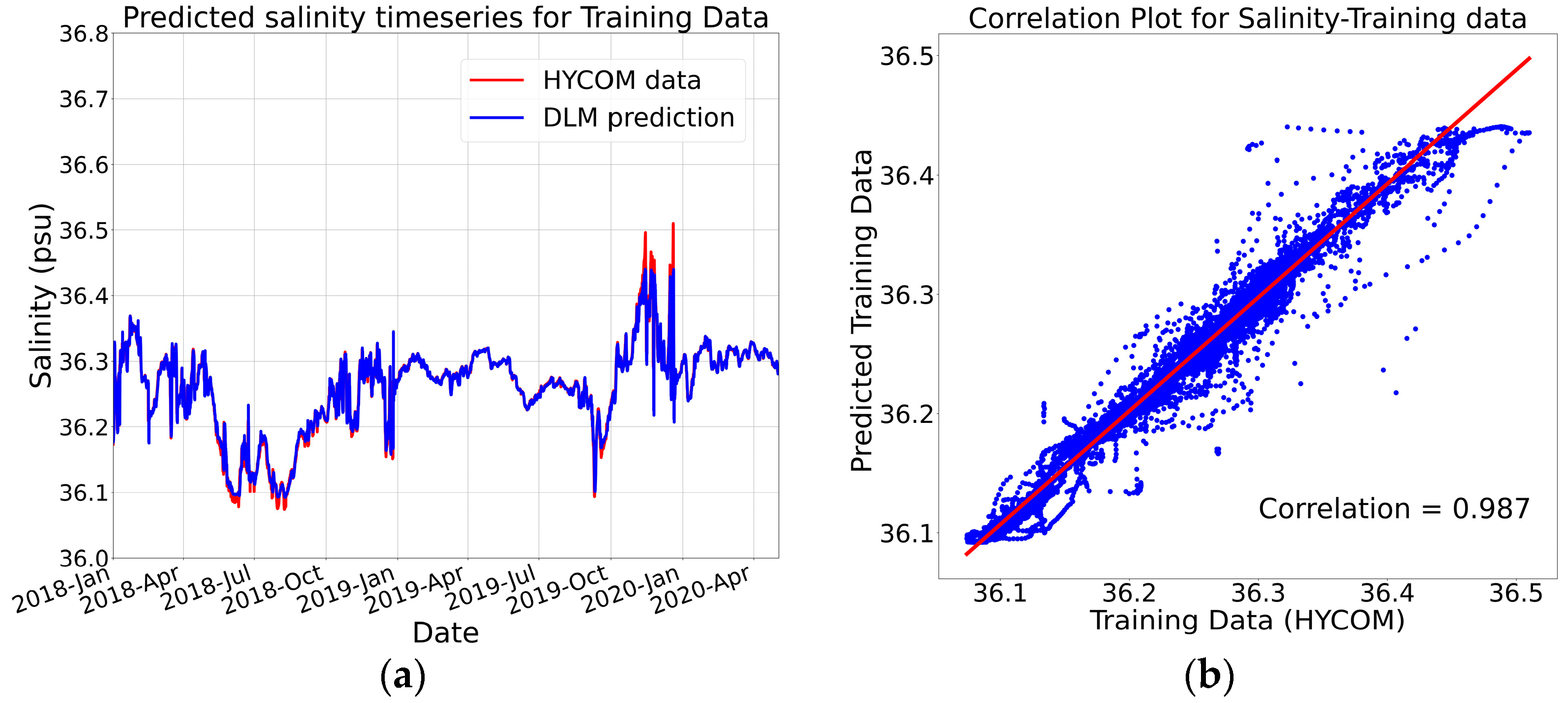
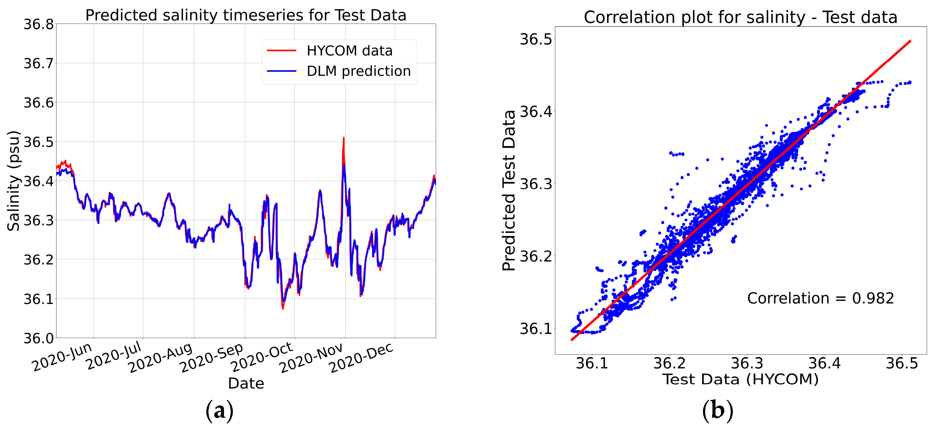
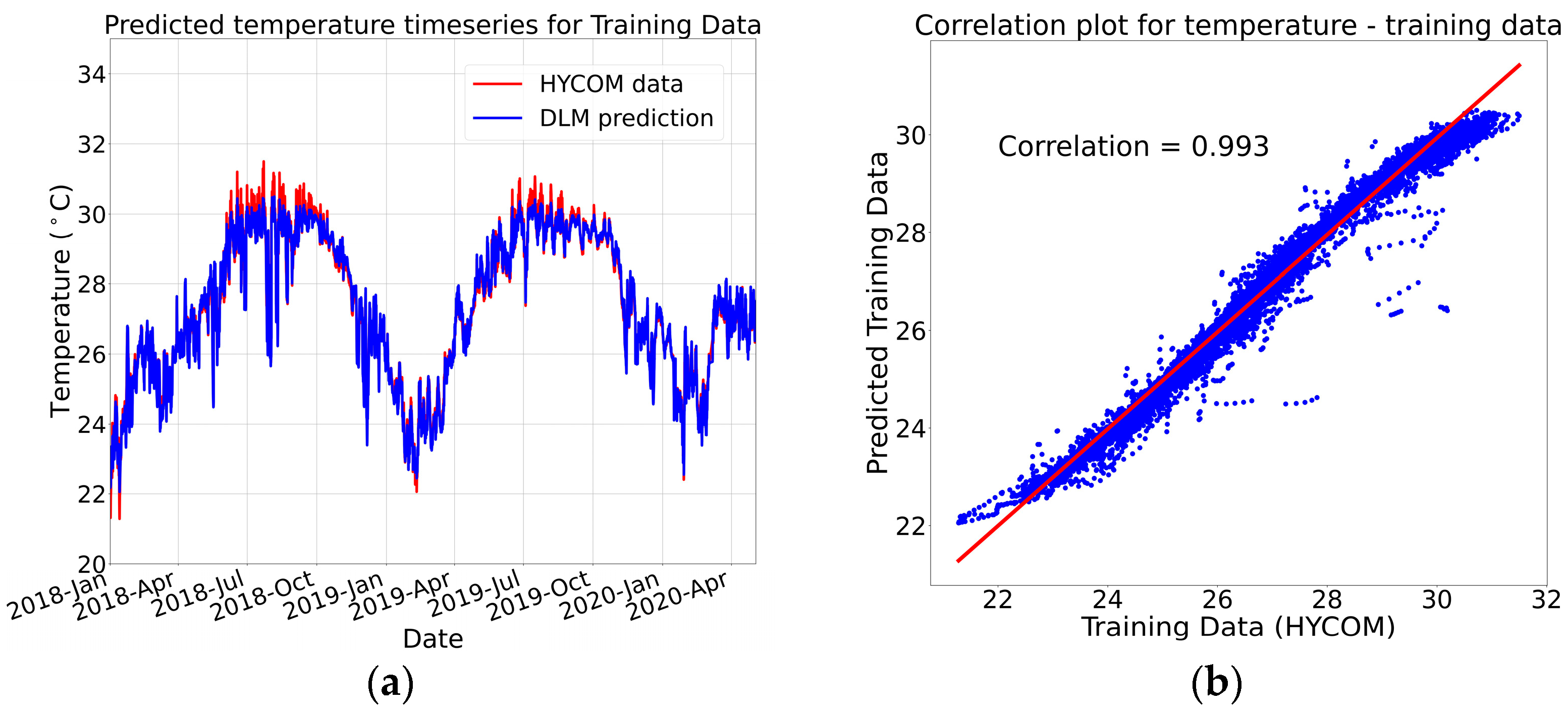
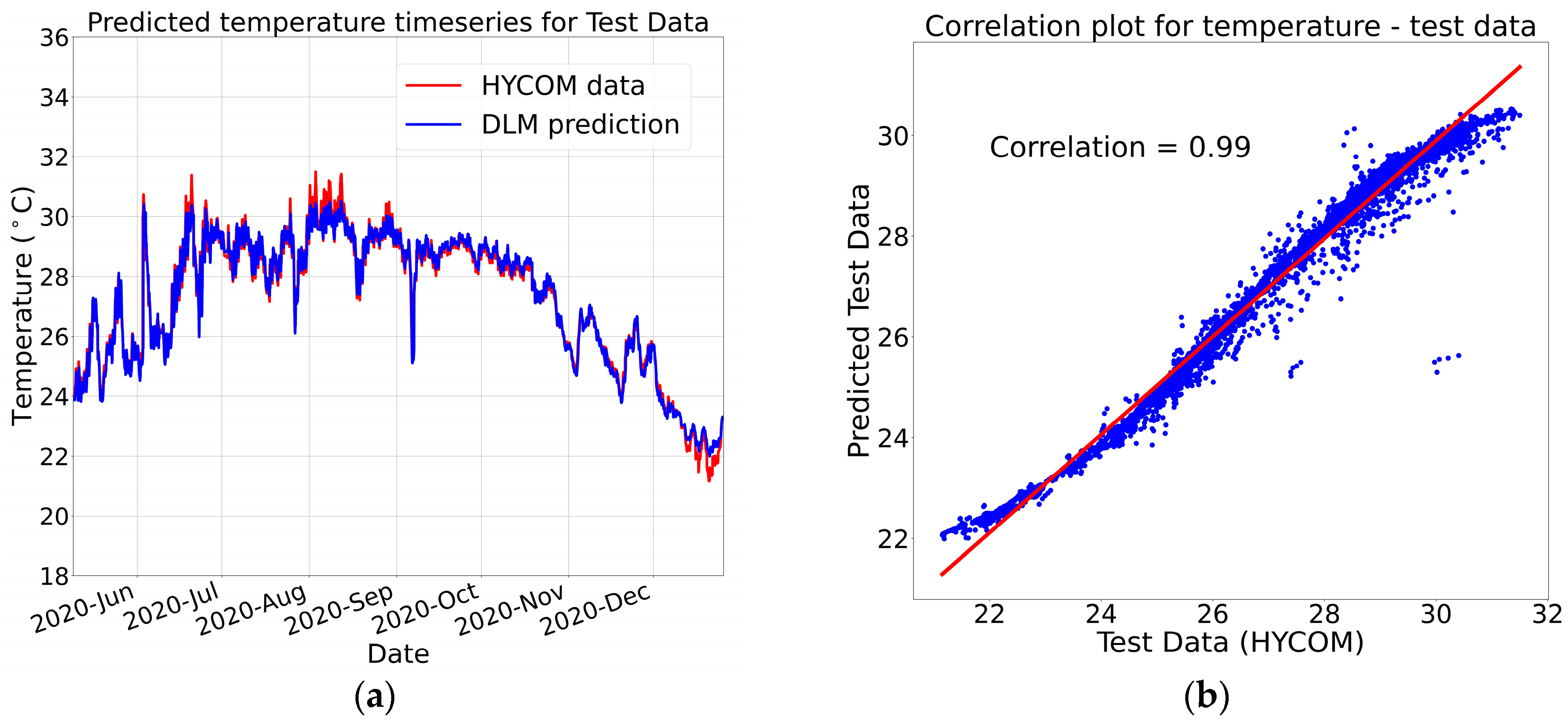
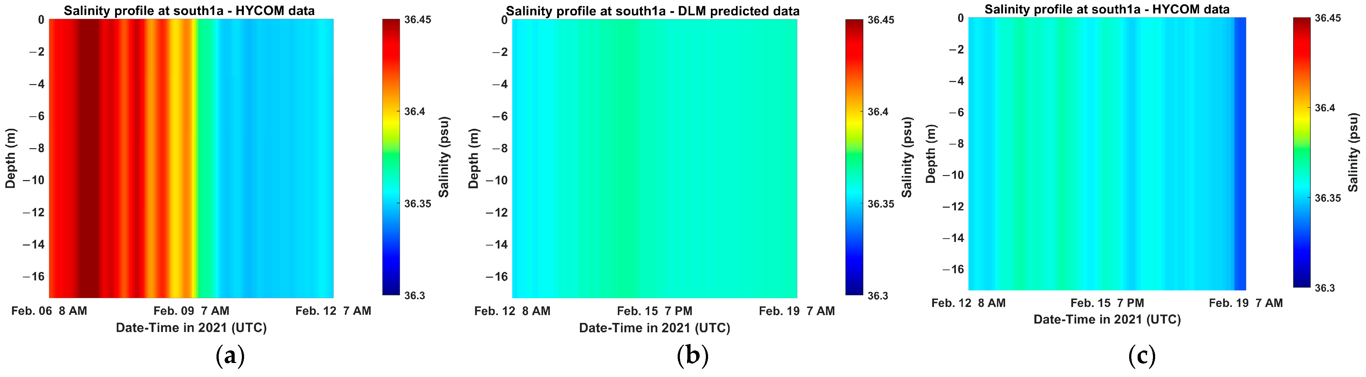
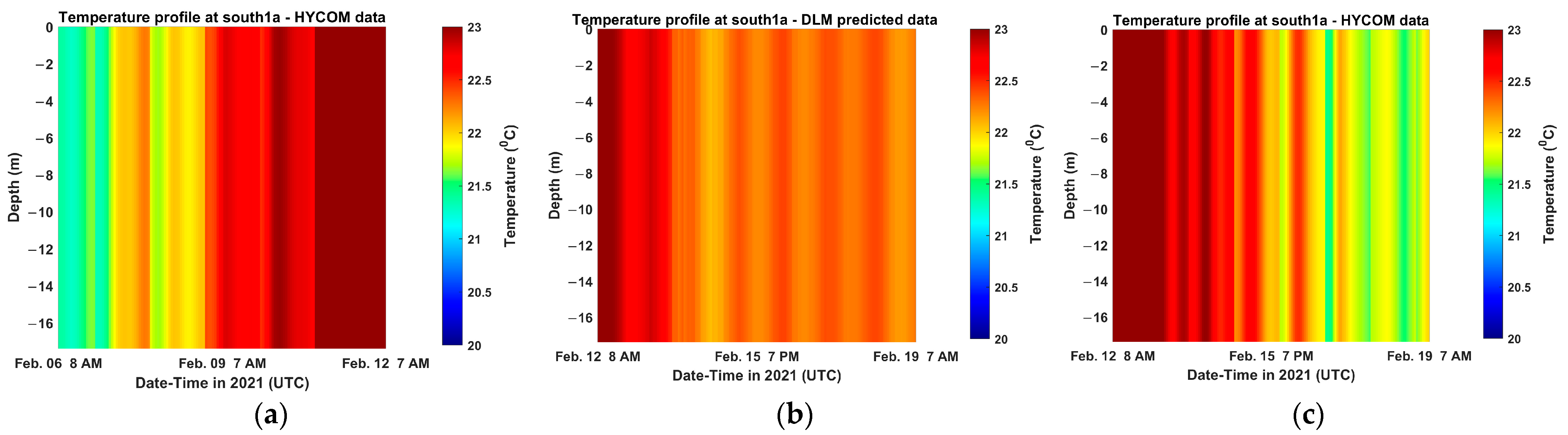
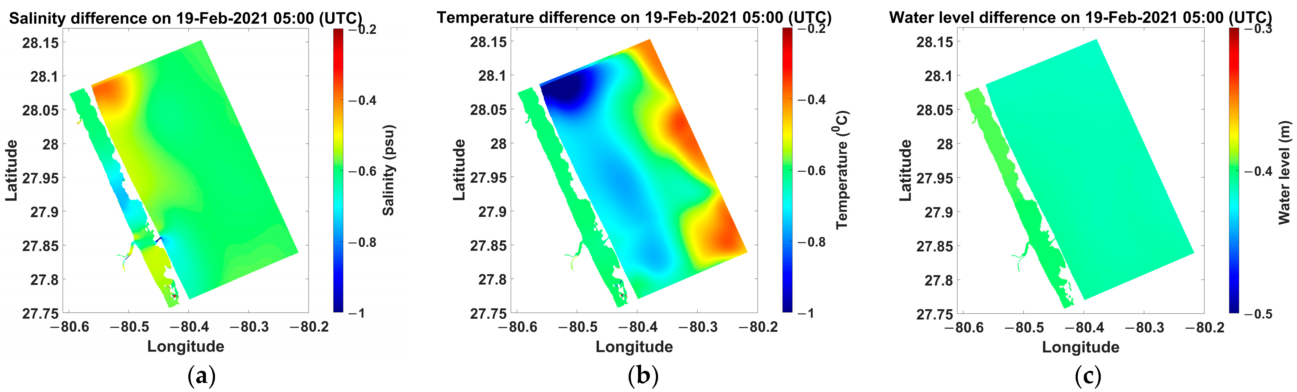
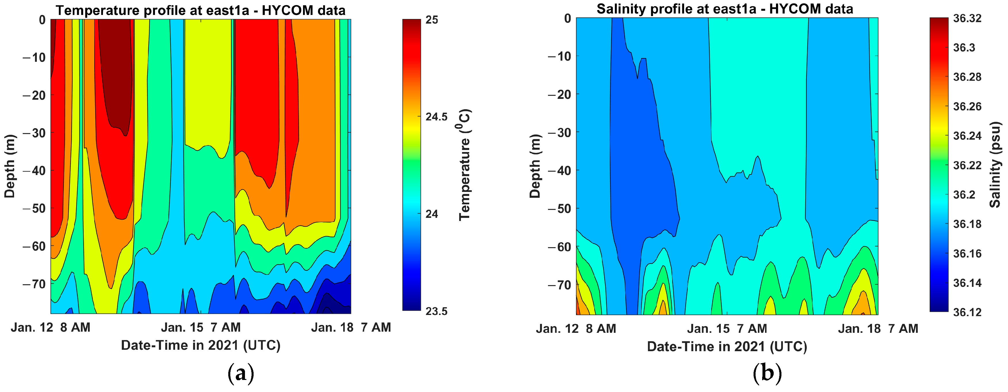
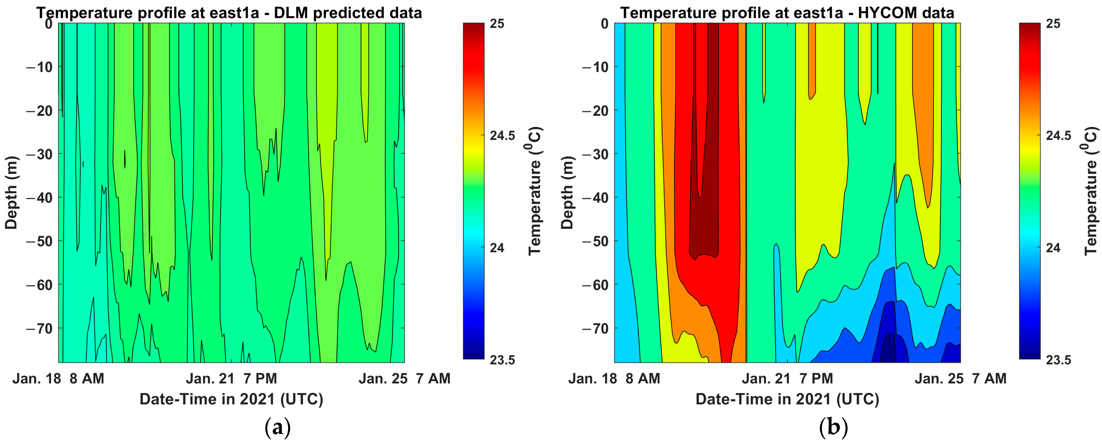
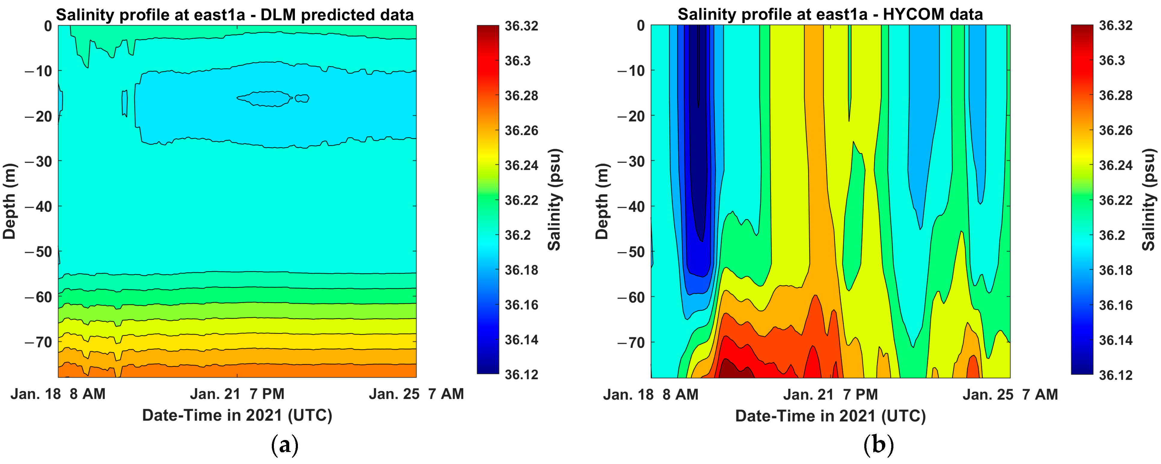
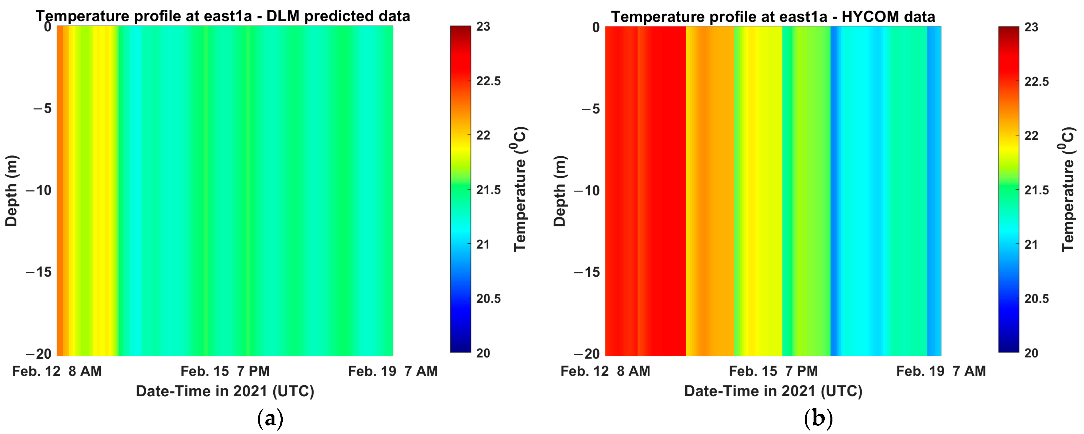
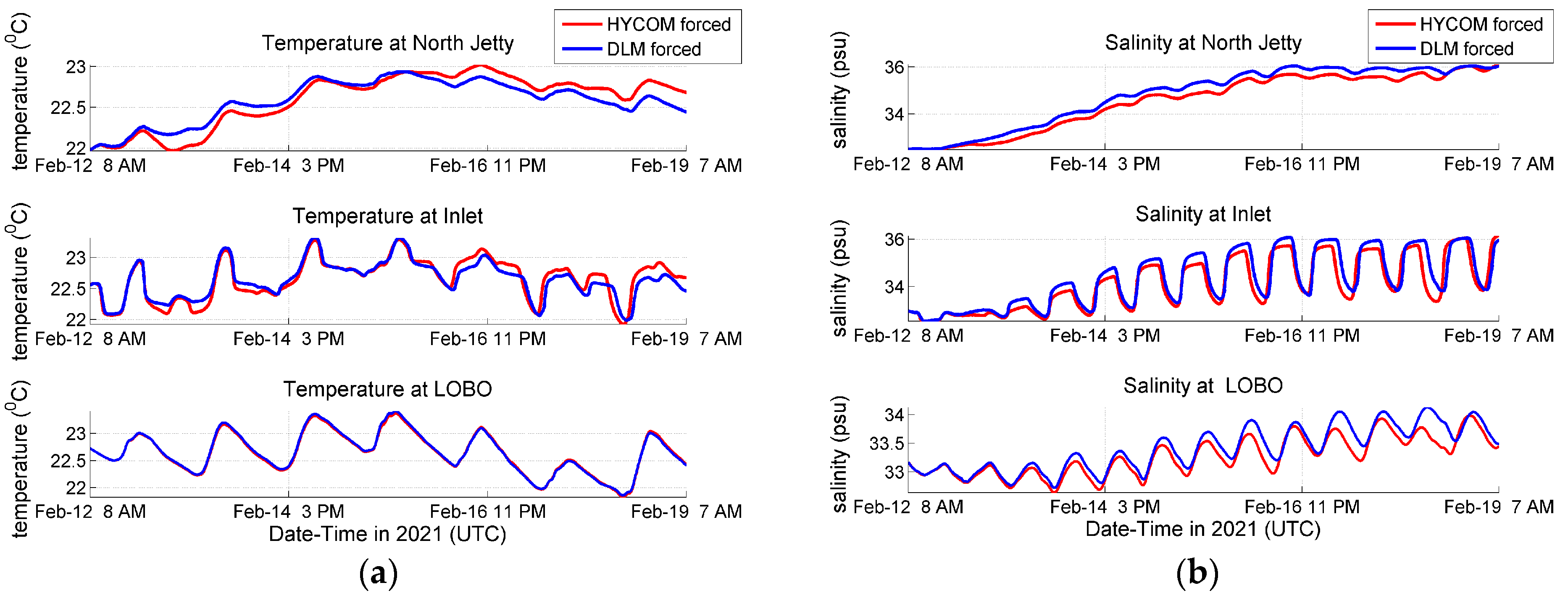
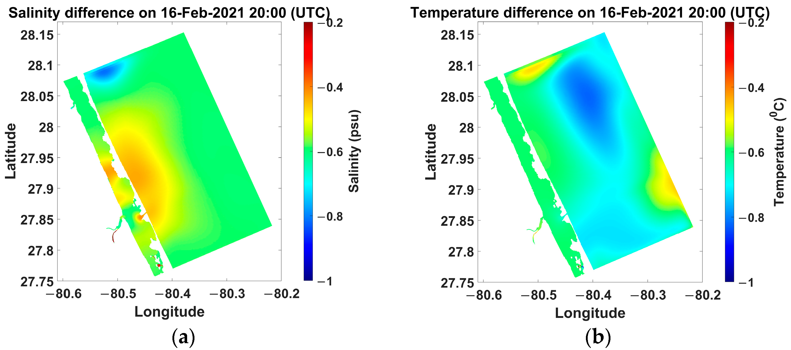
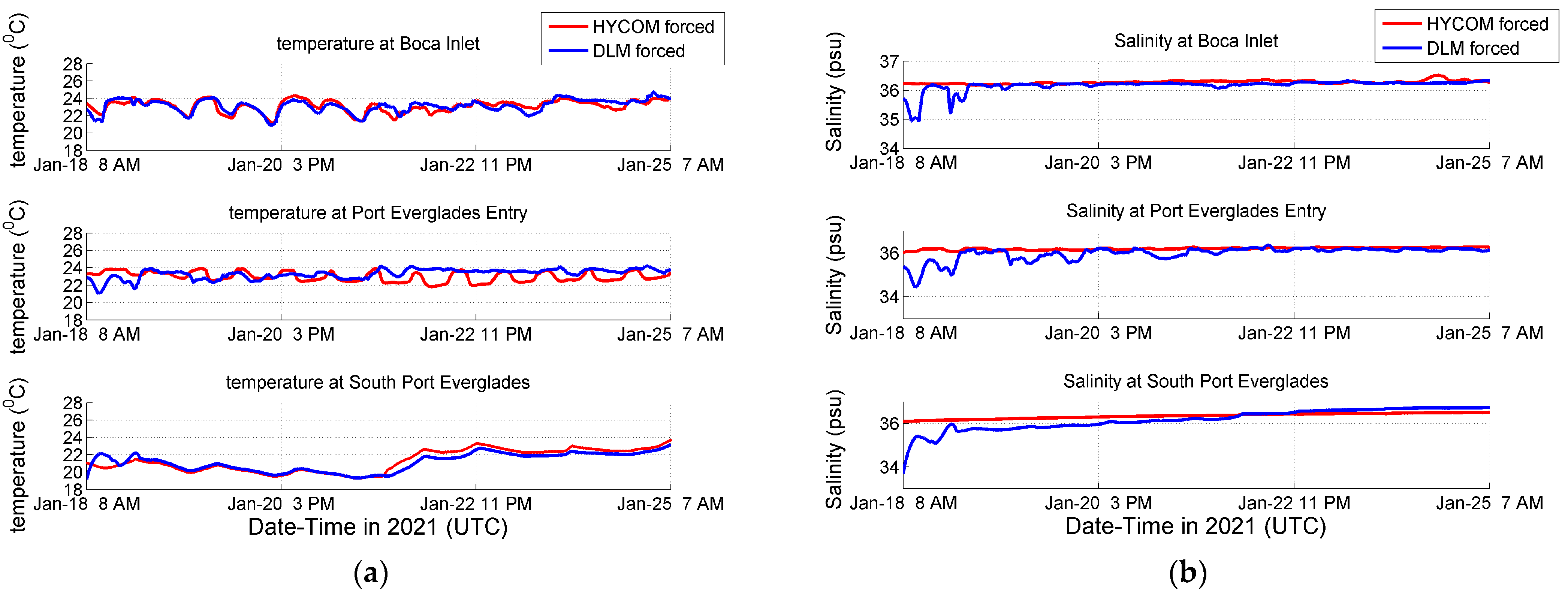
4.1. Salinity and Water Temperature

The comparison of salinity and water temperature outputs from the two simulations (DLM and HYCOM) exhibit similar patterns to the water level comparison. The salinity and water temperature data show a high degree of agreement for the first three days, indicating a near-perfect match between the predictions from the DLM and the HYCOM data-driven simulation (Figure 14). However, as the forecast period progresses beyond day three, the differences between the two simulations begin to increase.

The heat map plot in Figure 15a shows the salinity difference between the first simulation (DLM-predicted forecast) and the second simulation (HYCOM forced model). The salinity difference is large near the closed and open boundaries of the inlet and in geometrically constrained areas. This suggests that the DLM-predicted forecast might deviate from the HYCOM forced model in these regions. Figure 15b presents a water temperature difference heat map between the first and second simulations in the whole model domain. The DLM-predicted forecast model generally matches well with the HYCOM forced model throughout the model domain, except near the ocean boundaries where the water temperature difference is around 0.2 °C to 0.5 °C. This indicates that the DLM captures the water temperature variations well, but there might be discrepancies near the open ocean boundaries.

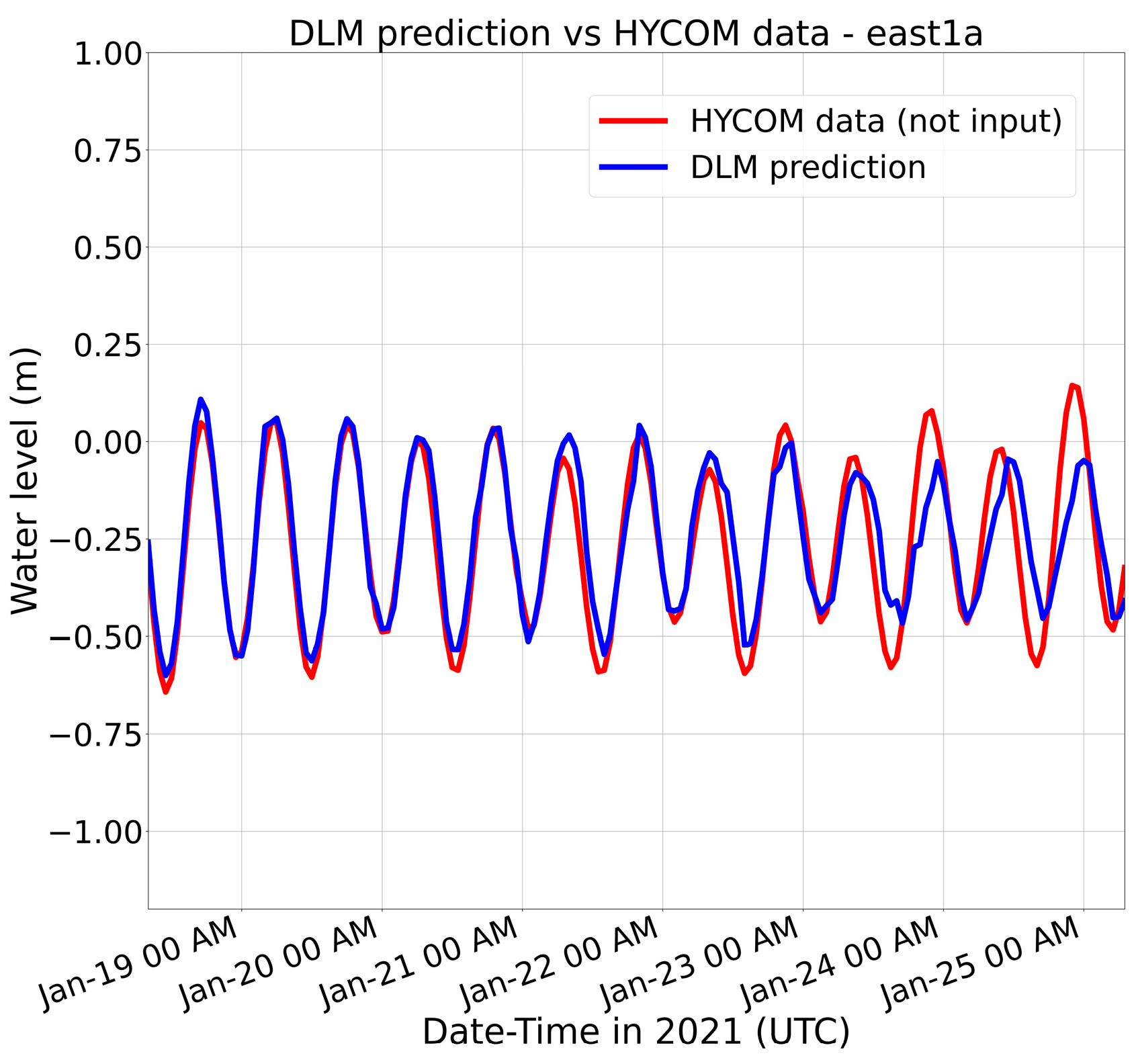
4.2. Water Level

The comparison of water level outputs from the first simulation (DLM-predicted data) and the second simulation (HYCOM data) at the three stations, North Jetty, LOBO, and Sebastian Inlet (see location in Figure 1b), reveal a close correspondence in the early days of the forecast period (Figure 16a). The water level of both simulations matches quite perfectly for the first three days. However, as the length of the forecast increases, deviations begin to emerge, and the differences between the two simulations become more significant.

The heat map of water level differences between the two simulations in Sebastian Inlet (Figure 16b) indicates that the water level difference is close to zero inside the estuary and coastal areas. However, there is a slight difference of approximately 0.01 m near the open ocean boundaries. This suggests that the DLM can accurately capture the water level variations within the estuary and coastal regions, but there might be discrepancies near the ocean boundaries.

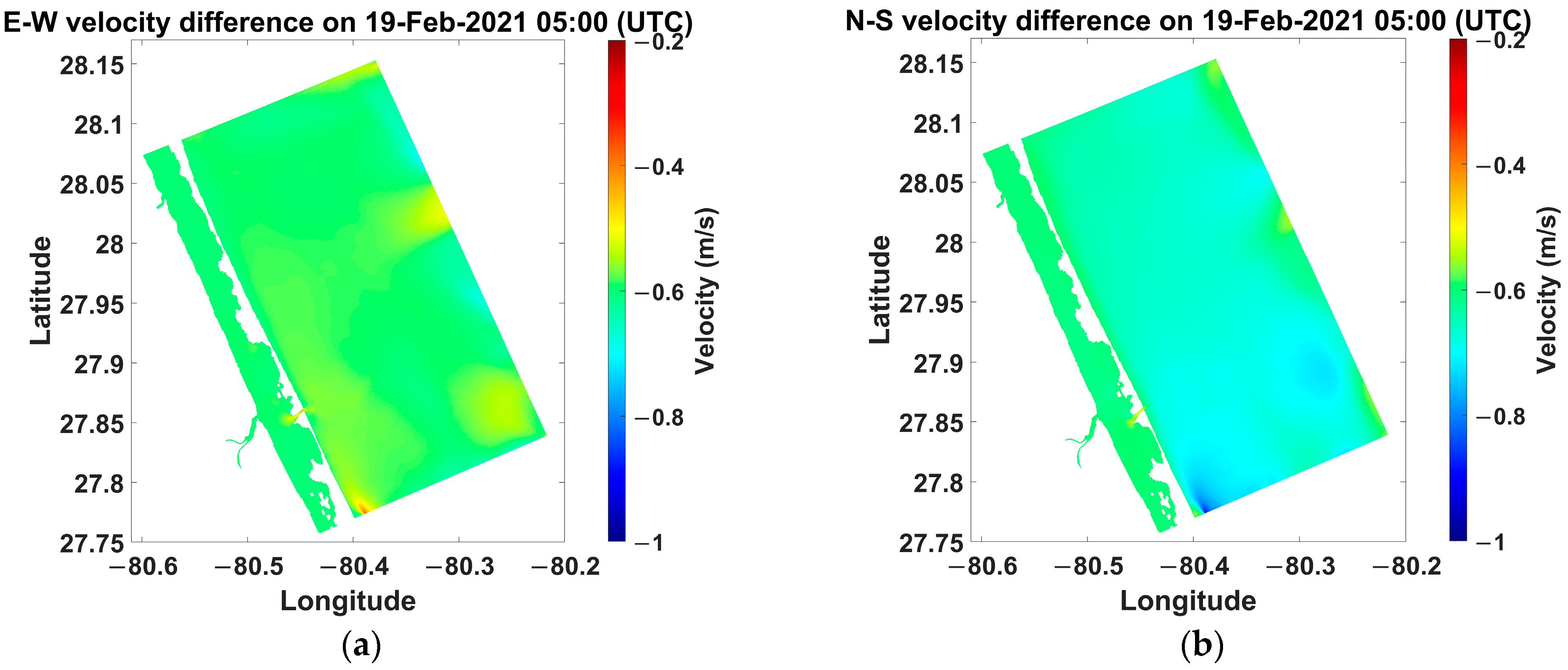
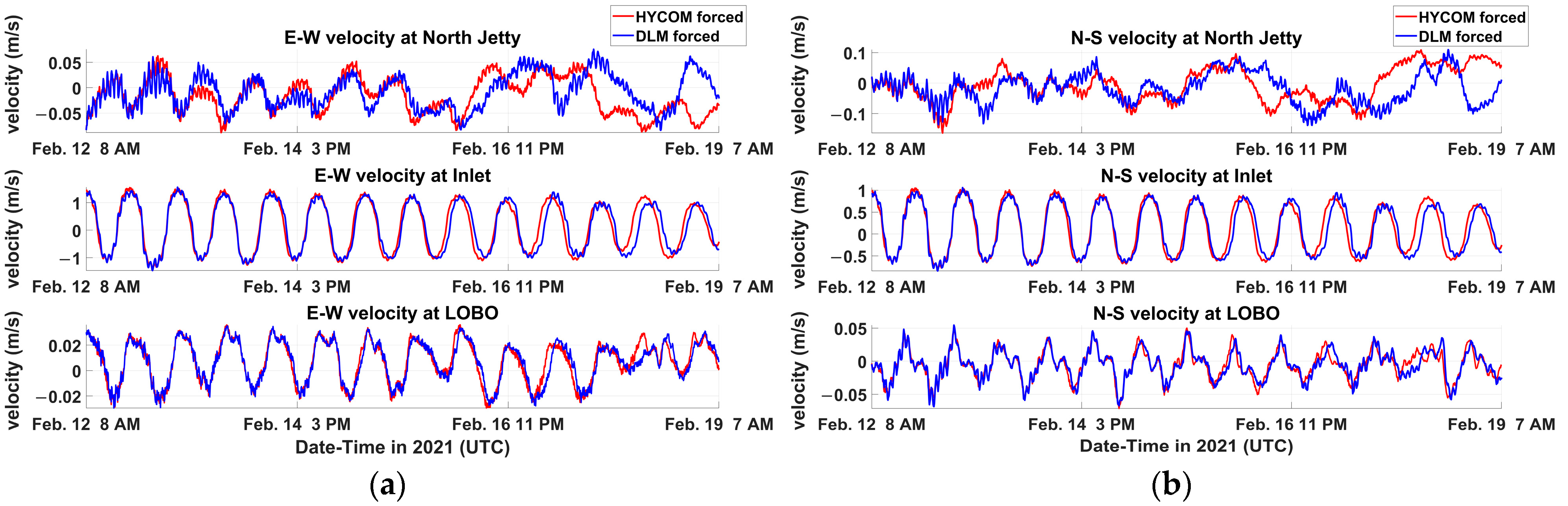
4.3. Currents

The velocity components from the first simulation with DLM-predicted data match well with the velocity components from the second simulation at all three stations: North Jetty, LOBO, and Inlet. At the LOBO and Inlet stations, the u and v components of velocity predicted by the DLM forced simulation show a good match with the second simulation, except for some differences towards the end of the prediction period (Figure 17). These comparisons suggest that the DLM predictions can capture the overall velocity patterns at these stations, aligning closely with the simulations using the HYCOM data. The discrepancy between the two simulations is larger at North Jetty station.

Figure 18 also presents the velocity component differences throughout the model domain (right panel). The difference in velocity is around 0 m/s over most of the model domain, indicating a good agreement between the DLM-predicted forecast and the HYCOM forced model. However, near the open ocean boundaries, there is a difference of approximately 0.1 m/s. Overall, these heat map plots highlight the performance of the DLM-predicted forecast model compared to the HYCOM forced model. Whereas the DLM method shows good agreement in many areas, there are some discrepancies near the open ocean boundaries and in geometrically constrained areas, particularly in terms of water level, velocity, salinity, and water temperature. These differences may be attributed to the complexity of the model domain and the limitations of the developed DLM in capturing fine-scale features and boundary effects accurately. Additional heat map plots have been included in Appendix A (Figure A7, Figure A8, Figure A9 and Figure A10).

4.4. Length of Prediction Range

The correlation coefficient analysis conducted for different time lengths reveals unique trends in the accuracy of the predictions (Figure 19). For the first 3 days, all parameters, including water level, salinity, water temperature, and the u-component and v-component of velocity, exhibit significantly high correlations, with values exceeding 96%. This indicates that the DLM-predicted forecasts closely match the HYCOM forced model during this initial period.

However, as the forecast length increases to the 4th and 5th days, the correlations show a slight decline compared to the first 3 days. Although still relatively high, there is a small decrease in the accuracy of the predictions during this period. The most notable decline in correlation occurs from the 6th day onwards. The correlations sharply fall, indicating a decrease in the accuracy of the predictions for all parameters. This decline is particularly prominent for salinity, where the correlation drops more significantly compared to other parameters.

These findings suggest that the DLM performs well in capturing the dynamics and patterns of the simulated variables for the first few days of the forecast. However, as the forecast length increases, the accuracy of the predictions gradually decreases, with a sharper decline observed from the 6th day onwards. This decline may be attributed to the limitations of the DLM in capturing long-term dependencies and the cumulative errors associated with the recursive method applied to obtain a multi-step forecast.

4.5. Direct Application

The flow DLM was applied to the Port Everglades model [20] to predict salinity, water temperature, and water level forecast data. Unlike the previous case where the DLM was trained with local data, in this scenario, the Flow DLM from the Sebastian model was applied directly without prior training with local data. Instead, the HYCOM salinity, water temperature, and water level data for the Port Everglades region were used as inputs to the DLM for prediction. Using the HYCOM data as inputs, the flow DLM generated predictions for salinity, water temperature, and water level for the Port Everglades model. These predictions are based on the learned patterns and relationships captured by the DLM from the available HYCOM data.

The purpose of applying the flow DLM directly to the Port Everglades model is to evaluate its performance in an unknown domain where it has not been specifically trained with site-specific data. This approach allows the study to assess how well the DLM can adapt and generalize to new locations or conditions without the need for local training data.

The comparison of water level outputs from both simulations at three observation stations, south Port Everglades station, Boca Inlet station, and the entrance point in Port Everglades (see location in Figure A11), shows a good correlation for the first 3 days. However, the differences between the two simulations increased from day 4, indicating a decrease in the accuracy of the DLM predictions as the forecast length extended (Figure 20).

The comparison of water temperature (Figure 21a) and salinity (Figure 21b) outputs at all three stations reveal similar patterns, with a good match for the first 3 days but increasing deviations afterward. The performance of the DLM in predicting salinity is notably lower compared to water level and water temperature. The DLM applied to the Port Everglades model does not perform as well as the DLM applied to the Sebastian model in terms of salinity and water temperature predictions.

The comparison of E-W (Figure 22a) and N-S velocity (Figure 22b) components at the Boca Inlet and Port Everglades entry stations shows better agreement compared to other stations. However, at the South Port Everglades station, particularly inside the harbor, there is a significant discrepancy in the u component of horizontal velocity. This discrepancy can be attributed to the geometrical constraints in the E-W direction, which result in a weaker u component. The magnified difference in this case may be due to the already marginal values of the u component.

The correlation coefficient comparison on different time scales indicates that the water level maintains a higher accuracy up to day 5 and does not significantly decrease compared to other parameters (Figure 23). This suggests that the DLM applied to the Port Everglades model performs relatively well in predicting water level dynamics. However, for other parameters such as salinity and water temperature, the correlations are weaker compared to water level. In terms of the E-W velocity component, the performance is better at Boca Inlet compared to South Port Everglades. The complex geometry of the South Port Everglades location, with its constraints in the E-W direction, may contribute to the higher discrepancy observed in the velocity component at that station. Overall, the correlation comparisons, except for water level, indicate relatively lower performance compared to the DLM applied to the Sebastian model. This emphasizes the need for retraining the DLM with local data to improve its performance in the Port Everglades model.

5. Real-Time Forecasts

A real-time forecast system has been developed using three different methods to ensure continuous forecast availability under various scenarios.

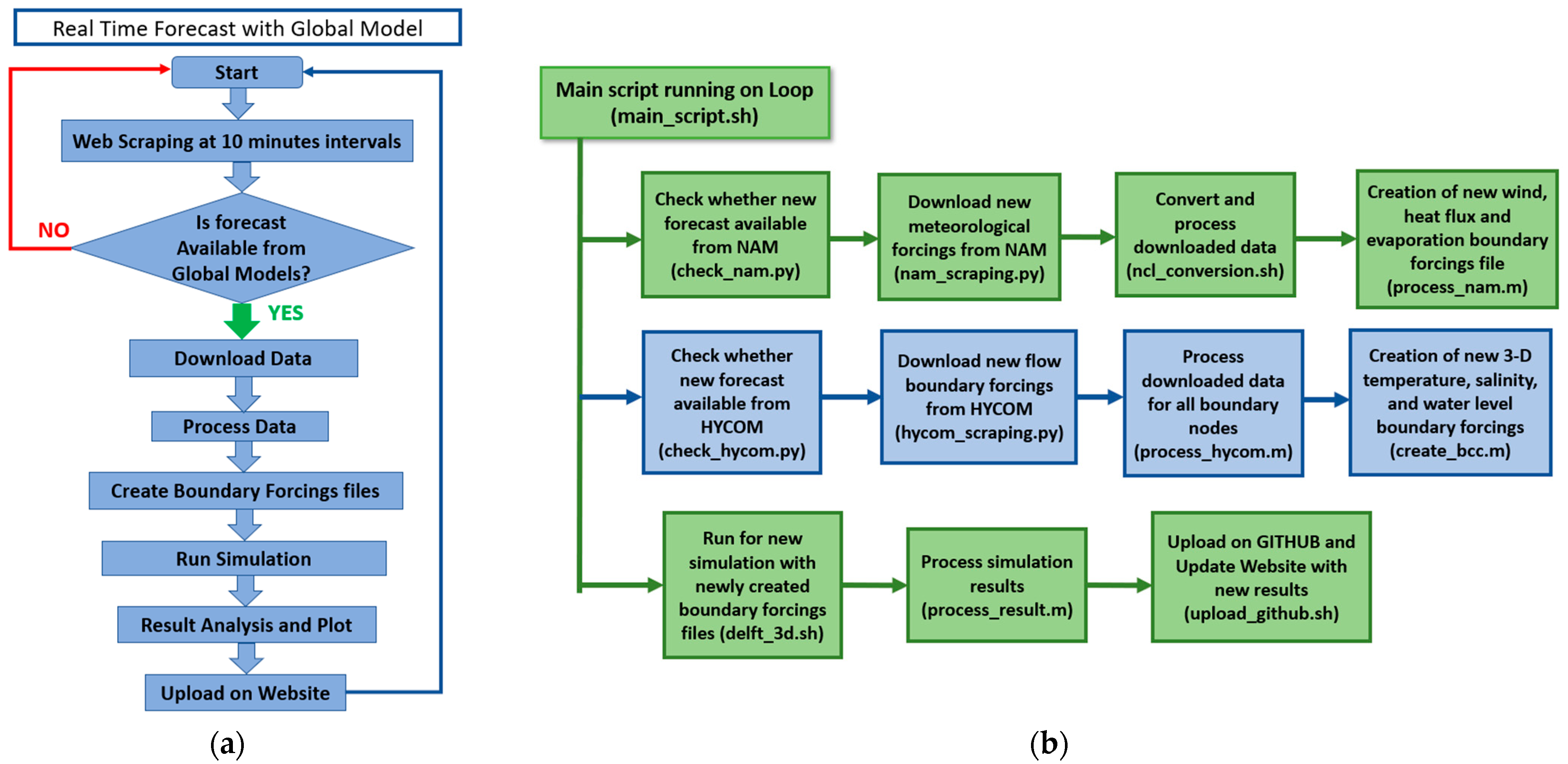
5.1. Real-Time Forecast with Data from Global Models

This method is employed when forecast data from global models are available. The system retrieves the forecast data from the global models, processes it, and uses it as boundary forcings for the forecast simulation. The results of the simulation are then analyzed and made available on a webpage.

For real-time forecasting, the calibrated model’s boundary conditions are updated using data from global models such as HYCOM [18] and NAM [21]. Python scripts employ web scraping techniques to extract necessary data from these models’ webpages. The downloaded data are processed using Python and MATLAB scripts to generate boundary conditions for the calibrated model. A new simulation of the model is then executed, incorporating the updated boundary conditions. The simulation output is processed to create time series plots at observation stations, which are uploaded to a public website. Each simulation uses a hot start file from the previous run for continuity. Automation and synchronization of scripts ensure periodic checks for new data, facilitating seamless updates every 10 min (Figure 24a).

The entire process is managed through a combination of bash, MATLAB, and Python scripts, coordinated by ‘main script.sh’. It oversees activities including data acquisition, creating boundary conditions, executing simulations, and post-processing model results (depicted in Figure 24b). New data availability from NAM is determined by ‘check nam.py’ via web scraping, with subsequent download and conversion using ‘nam_scraping.py’ and ‘ncl_conversion.sh’. MATLAB script ‘process_nam.m’ generates meteorological boundary conditions, ‘check hycom.py’ detects new HYCOM data, downloaded by ‘hycom_scraping.py’ processed into flow boundary conditions using MATLAB scripts (‘process_hycom.m’ and ‘create_bcc.m’). The ‘delft3d.sh’ script initiates a new simulation, followed by ‘process_result.m’ for post-processing and visualization. Finally, ‘run_github.sh’ and ‘upload_github.sh’ scripts transfer files to GitHub, uploading them onto the GitHub webpage (see the Supplementary Materials).

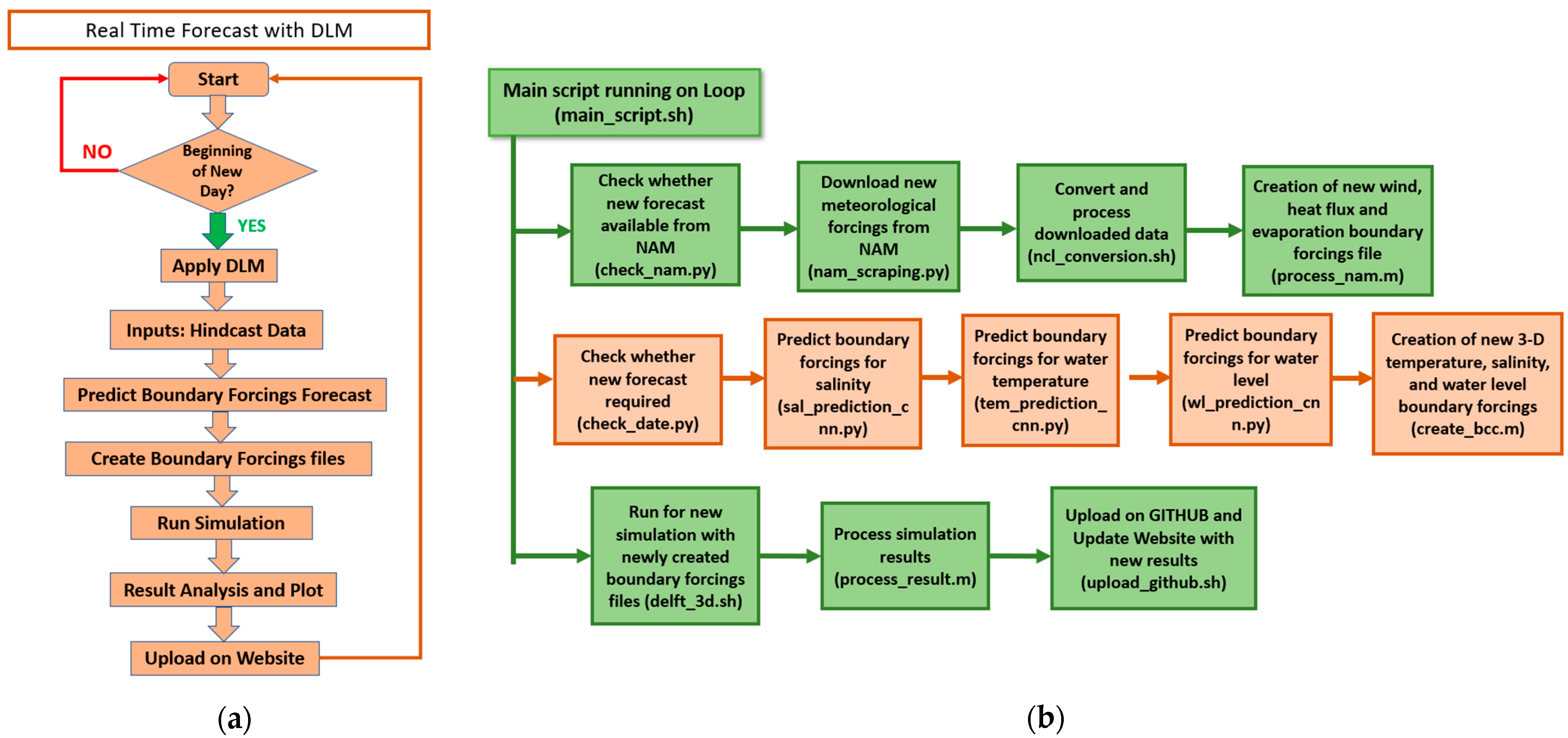
5.2. Real-Time Forecast with DLM

In the absence of a global model with forecast data, the DLMs are employed as an alternative for generating boundary forcings in estuarine and coastal areas. To ensure continuous forecast simulations, an automated system runs daily simulations using hindcast data as inputs for the DLM, predicting necessary boundary forcings. The generated forcings file initiates a new simulation, and the system analyzes and uploads the results to a designated webpage (Figure 25a). This process is coordinated through bash, MATLAB, and Python scripts, with ‘main_script.sh’ orchestrating activities like creating boundary conditions, running simulations, and post-processing results. Python scripts such as ‘sal_prediction_cnn.py’, ‘tem_prediction_cnn.py’, and ‘wl_prediction_cnn.py’ predict flow boundary conditions. MATLAB scripts these predictions to create boundary forcings, initiating a new simulation using ‘delft3d.sh’ and post-processing with ‘process_result.m’. Finally, ‘run_github.sh’ and ‘upload github.sh’ transfer files to a GitHub folder and upload them to the GitHub webpage (Figure 25b).

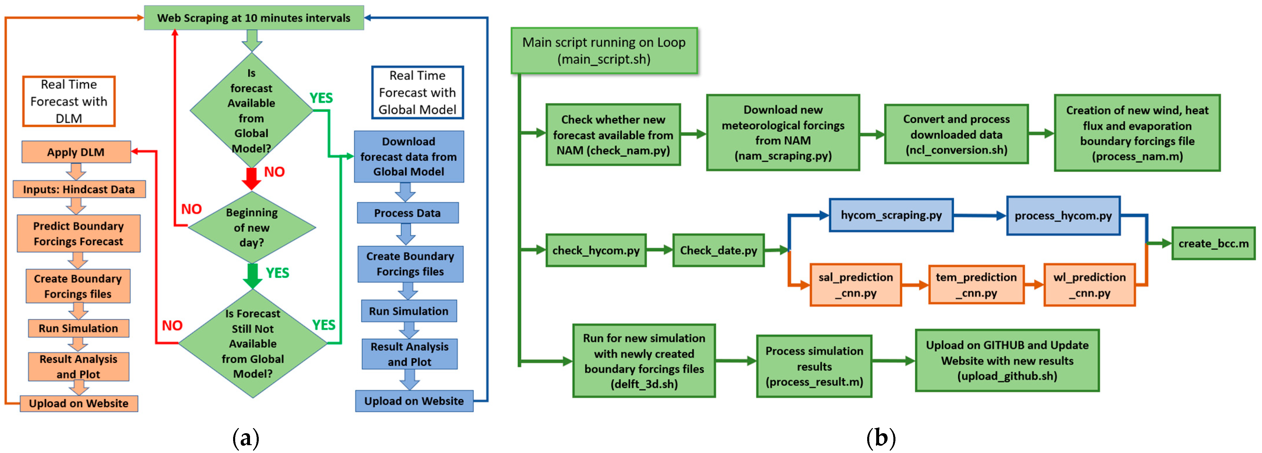
5.3. Real-Time Forecast with a Combination of Global Models and DLM

In cases where the global forecast model is intermittently unavailable, a hybrid approach is employed. The system first checks for the availability of forecast data from the global models. If the data are accessible, it is used as boundary forcings as described in Section 5.1. However, if the global model is down, the system switches to the DLM method as described in Section 5.2. This combination ensures that forecast data are provided even when the global model experiences disruptions. By implementing these three methods in the real-time forecast system, forecast availability is ensured in various scenarios, including situations where global forecast data are available, unavailable, or intermittently unavailable (Figure 26a). In the hybrid approach, the automation system checks for new forecast data every 10 min from global models such as HYCOM and NAM models through web scraping. If global model data are available (Method 1), it downloads and processes HYCOM data using specific scripts (‘hycom_scraping.py’, ‘process_hycom.m’, ‘create_bcc.m’, and ‘mdcreate.m’). If no new global model data are available on a new day, it switches to Method 2, using the DLM technique. Scripts (‘sal_prediction_cnn.py’, ‘tem_prediction_cnn.py’, ‘wl_prediction_cnn.py’) apply DLMs using hindcast data from HYCOM to predict boundary conditions. Once boundary forcings files are prepared with either Method 1 or Method 2, simulations run with ‘delft3d.sh’, results are analyzed with ‘process_result.m’, and the analysis is uploaded to the webpage using ‘upload_github.sh’. This hybrid approach ensures continuous forecast data generation, utilizing global model data when accessible and switching to DLM predictions when not (Figure 26b).

6. Discussion

In this study, a three-dimensional numerical model has been developed using Delft3D to simulate hydrodynamics in the central IRL of the Florida Atlantic coast (Figure 1). This model has been constructed with a high spatial resolution specifically focused on the Sebastian Inlet areas (Figure 1 and Figure 2). The model is driven by water elevation time series, which includes tides and lower frequency sea level oscillations, meteorological forcing, and flow and transport boundary conditions. To ensure the accuracy of the model, key parameters including water level, tide, salinity, water temperature, and currents are evaluated against observed data. A DLM has been developed using the CNN method to obtain required boundary conditions data, including water level, water temperature, and salinity, for creating a real-time forecast model. The DLM is trained and tested with two distinct datasets to eliminate bias in the testing phase. During the training and testing period, the DLM provides two-step predictions for each parameter, considering the strong correlation observed in the partial autocorrelation up to two lag features.

To accomplish multi-day forecasting, a recursive strategy is employed to create a multi-step forecast model. Utilizing this DLM, a 7-day forecast for flow boundary conditions (water level, salinity, and water temperature) is generated (Figure 8, Figure 9 and Figure 10). These predictions from DLMs are validated by running two separate Delft3D flow simulations, one with DLM-predicted boundary conditions and another with boundary conditions derived from HYCOM (Figure 11, Figure 12 and Figure 13). The simulation outputs, including water level, salinity, water temperature, and the E-W and N-S horizontal velocity components, are compared with simulations with HYCOM data at three observation points: Sebastian Inlet, North Jetty, and LOBO station (Figure 14, Figure 15, Figure 16, Figure 17 and Figure 18).

The comparison of correlation coefficients for different time lengths reveals that the results from simulations using DLM-predicted forcings correlate very well with the results from simulations using the global model’s forecast data for up to the first 5 days, achieving an accuracy of over 90% (Figure 19). This demonstrates that even in the absence of hindcast data up to 4 days prior to the forecast beginning time, the real-time forecast with DLM can still achieve an accuracy above 70% for 3 days of the real-time forecast with global model data.

Whereas the DLM demonstrates good agreement in most areas of the model domain, there are discrepancies, particularly near ocean boundaries and in geometrically constrained areas. The differences observed near the open ocean boundaries can be attributed to several factors, including the presence of boundary effects and limitations of the developed DLM. To address these prominent discrepancies near the ocean boundaries, several potential strategies can be considered, such as placing the open boundaries further offshore could help ensure that the boundary conditions are representative of the offshore conditions. The developed DLM is also applied directly to the Port Everglades model, even though it has not been trained with Port Everglades area data. The input for this DLM prediction is HYCOM hindcast data for the Port Everglades region. Two separate simulations are run, one using HYCOM forecast data and another using DLM-predicted forecast data. The results from these simulations are compared through time series and correlation analysis. The simulated water level and velocity components from these two simulations correlate quite well (Figure 20, Figure 21, Figure 22 and Figure 23). However, the simulated salinity and water temperature do not perform as well as the Sebastian Inlet model, highlighting the challenge of predicting these parameters accurately. This comparison underscores the importance of training the DLM with local data for more accurate outcomes.

A real-time forecast system has been developed for the Sebastian Inlet area, which provides forecasts for water level, salinity, current, and water temperature for up to 3 days. This forecast system utilizes the calibrated model and operates in an automated manner, where updated boundary conditions, simulations, plotting, and website updating are accomplished without any manual effort. Synchronized scripts have been developed to automate all routine model tasks, ensuring seamless operation of the forecast system. This real-time forecast system has been successfully running since 2019 and continues to provide forecasts to date. The real-time forecast system is designed to accommodate three different scenarios. In the first scenario, when data from global models are available, real-time forecasts are generated using the global model data (Figure 24). In the second scenario, when global forecast model data are unavailable, the real-time forecast system relies on the DLM approach to provide forecast data (Figure 25). Lastly, in the third scenario, when the global forecast model is intermittently down, the real-time forecast system combines both methods to ensure continuous and reliable forecasts (Figure 26). These three methods provide flexibility and robustness to the real-time forecast system, enabling accurate forecasts even in challenging data availability scenarios.

7. Conclusions

The DLM developed in this study demonstrated high accuracy in predicting salinity, water temperature, currents, and water level data. The forecast using this DLM showed a strong correlation with the simulation using the Global model data. However, the accuracy of the predictions decreased as the timescale increased, which may be attributed to propagation errors associated with recursive methods. Nevertheless, the DLM developed in this study performed well in achieving the desired 3-day forecast data.

When directly applying the Sebastian Inlet DLM to the Port Everglades model, the simulation of water level yielded satisfactory results. However, the accuracy for currents, salinity, and water temperature was not as high. This emphasizes the need to retrain the DLM using local data to improve its performance and achieve higher accuracy for these parameters.

The development of the DLM in this study has addressed the challenge of limited forecast data availability in coastal and estuarine modeling, particularly for multi-day forecasting. This study provides comprehensive documentation of the concept, detailed methods, model development, performance evaluation, and application of the DLM and nested model approach in estuarine and coastal modeling. The findings and methodologies presented in this study can serve as a valuable framework for future research, development, and implementation of real-time forecast modeling systems in estuarine and coastal areas where forecast data are limited or unavailable. The data-driven approach employed in this study, supplemented by numerical modeling, has demonstrated its effectiveness in improving forecast accuracy and overcoming data limitations.

References

- Ezer, T.; Atkinson, L.P.; Corlett, W.B.; Blanco, J.L. Gulf Stream’s induced sea level rise and variability along the us mid-Atlantic coast. J. Geophys. Res. Ocean 2013, 118, 685–697. [Google Scholar] [CrossRef]
- Katavouta, A.; Thompson, K.R. Downscaling Ocean conditions: Experiments with a quasi-geostrophic model. Ocean Model. 2013, 72, 231–241. [Google Scholar] [CrossRef]
- Katavouta, A.; Thompson, K.R.; Lu, Y.; Loder, J.W. Interaction between the tidal and seasonal variability of the Gulf of Maine and Scotian Shelf region. J. Phys. Oceanogr. 2016, 46, 3279–3298. [Google Scholar] [CrossRef]
- Auclair, F.; Estournel, C.; Marsaleix, P.; Pairaud, I. On coastal ocean embedded modeling. Geophys. Res. Lett. 2006, 33, 14. [Google Scholar] [CrossRef]
- Beckers, J.M.; Brasseur, P.; Nihoul, J. Circulation of the western mediterranean: From global to regional scales. Deep Sea Res. Part II Top. Stud. Oceanogr. 1997, 44, 531–549. [Google Scholar] [CrossRef]
- Cailleau, S.; Fedorenko, V.; Barnier, B.; Blayo, E.; Debreu, L. Comparison of different numerical methods used to handle the open boundary of a regional ocean circulation model of the Bay of Biscay. Ocean Model. 2008, 25, 1–16. [Google Scholar] [CrossRef]
- Penven, P.; Debreu, L.; Marchesiello, P.; McWilliams, J.C. Evaluation and application of the ROMS 1-way embedding procedure to the central California upwelling system. Ocean Model. 2006, 12, 157–187. [Google Scholar] [CrossRef]
- Tomczak, M. Shelf and Coastal Oceanography; University of Maine: Orono, ME, USA, 1998. [Google Scholar]
- Asefa, T.; Kemblowski, M.; McKee, M.; Khalil, A. Multi-time scale stream flow predictions: The support vector machines approach. J. Hydrol. 2006, 318, 7–16. [Google Scholar] [CrossRef]
- Guilford, T.; Meade, J.; Willis, J.; Phillips, R.A.; Boyle, D.; Roberts, S.; Collett, M.; Freeman, R.; Perrins, C.M. Migration and stopover in a small pelagic seabird, the Manx shearwater Puffinus puffinus: Insights from machine learning. Proc. R. Soc. B Biol. Sci. 2009, 276, 1215–1223. [Google Scholar] [CrossRef] [PubMed]
- James, S.C.; Zhang, Y.; O’Donncha, F. A machine learning framework to forecast wave conditions. Coast. Eng. 2018, 137, 1–10. [Google Scholar] [CrossRef]
- Krinitskiy, M.A. Application of machine learning methods to the solar disk state detection by all-sky images over the ocean. Oceanology 2017, 57, 265–269. [Google Scholar] [CrossRef]
- Bolton, T.; Zanna, L. Applications of deep learning to ocean data inference and subgrid parameterization. J. Adv. Model. Earth Syst. 2019, 11, 376–399. [Google Scholar] [CrossRef]
- Habib, M.A.; Zarillo, G.A. Gulf Stream Effects on Sea Level Oscillations: Enhancing Performance of a Coastal and Estuarine Model Nested into Global Model through Modified Boundary Conditions. J. Mar. Sci. Eng. 2024, 12, 775. [Google Scholar] [CrossRef]
- Deltares, D. Simulation of Multi-Dimensional Hydrodynamic Flows and Transport Phenomena, Including Sediments; Version 4.05; Delft3D-Flow User Manual: Delft, The Netherlands, 2022; Available online: https://oss.deltares.nl/web/delft3d/manuals (accessed on 16 February 2023).
- Google Earth Version 9.185.0.0. Sebastian, Florida, USA. Available online: https://earth.google.com/ (accessed on 13 April 2024).
- NOAA National Geophysical Data Center. 1/3 Arc-Second MHW Coastal Digital Elevation Model; NOAA National Centers for Environmental Information: Palm Beach, FL, USA, 2010. Available online: https://www.ncei.noaa.gov/access/metadata/landing-page/bin/iso?id=gov.noaa.ngdc.mgg.dem:427 (accessed on 25 April 2018).
- Metzger, E.J.; Helber, R.W.; Hogan, P.J.; Posey, P.G.; Thoppil, P.G.; Townsend, T.L.; Wallcraft, A.J.; Smedstad, O.M.; Franklin, D.S.; Zamudo-Lopez, L.; et al. Global Ocean Forecast System 3.1 Validation Testing; NRL Report; Naval Research Lab Stennis Detachment Stennis Space Center: Bay St. Louis, MS, USA, 2017; NRL/MR/7320-17-9722; Available online: https://hycom.org (accessed on 24 March 2023).
- Mesinger, F.; DiMego, G.; Kalnay, E.; Mitchell, K.; Shafran, P.C.; Ebisuzaki, W.; Jović, D.; Woollen, J.; Rogers, E.; Berbery, E.H.; et al. North American Regional Reanalysis: A long-term, consistent, high-resolution climate dataset for the North American domain, as a major improvement upon the earlier global reanalysis datasets in both resolution and accuracy. Bull. Am. Meteorol. Soc. 2006, 87, 343–360. [Google Scholar] [CrossRef]
- Habib, M.A.; Zarillo, Z.A. Construction of a Real-Time Forecast Model for Coastal Engineering and Processes Nested in a Basin Scale Model. J. Mar. Sci. Eng. 2023, 11, 1263. [Google Scholar] [CrossRef]
- NOAA North American Mesoscale Forecast System (NAM). Available online: https://registry.opendata.aws/noaa-nam (accessed on 24 March 2023).
- Google Earth, Version 9.185.0.0. Port Everglades, Florida, USA. Available online: https://earth.google.com (accessed on 20 May 2022).