Understanding Salinity Intrusion and Residence Times in a Small-Scale Bar-Built Estuary under Drought Scenarios: The Maipo River Estuary, Central Chile

Abstract

The Maipo River estuary is a low-inflow bar-built estuary that includes a protected wetland, which harbors a rich ecosystem. The estuary and wetland have been threatened by a persistent drought for more than a decade, which has resulted in greater salinity intrusion and increased residence times. Previous studies have described salinity and pollutants in estuaries; however, almost all have focused on deeper and/or wider estuaries with dimensions much larger than those of the small-scale Maipo River estuary. In this study, we used the numerical model FVCOM to simulate the dynamics of the Maipo River estuary under drought scenarios and explored the interactions between river discharge and tides in terms of saline intrusion and particle dispersal. The model was validated against observations collected during a field campaign near the river mouth. The simulations successfully reproduced the water surface elevation but underestimated salinity values, such that the vertical salinity structure observed in the field was not captured by the model in this shallow and morphologically complex estuary. Consequently, our model results provide qualitative insight related to salinity and baroclinic dynamics. Results of maximum saline intrusion showed an exponential decay with increasing river discharge, and the analysis of salinity intrusion time series revealed that droughts may cause permanent non-zero salinity levels in the estuary, potentially affecting ecological cycles. The incorporation of passive tracers showed that decreasing river discharge increases the residence time of particles by allowing the tracers to re-enter the estuary. Model results showed the formation of accumulation zones (hotspots) in the shallower zones of the estuary.

1. Introduction

Estuaries represent dynamic and fluctuating environments where tides and freshwater inflow interact, shaping their unique ecological characteristics [1]. These complex habitats harbor various plant and animal species, including fish, birds, and shellfish [2]. Estuaries play crucial roles in nutrient cycling and coastal sediment budgets and provide essential ecosystem services such as water purification and flood protection [3,4]. However, these habitats face increasing threats from factors such as droughts, which may elevate salinity levels and residence times, exacerbating ecological stressors [5,6]. Despite numerous studies exploring the dynamics of large and medium-sized estuaries [7,8,9,10,11,12,13], a notable research gap persists regarding small-scale estuarine systems. In these smaller systems, which are numerous worldwide [14,15,16], disruptions in river discharge or human interventions can have pronounced local effects, warranting further investigation to enhance our understanding of their ecological dynamics and conservation needs.

In Chile, the Maipo River mouth is a small-scale yet significant estuary, primarily recognized for its role in harboring a protected wetland that provides a habitat for delicate species of migratory birds [17]. Additionally, the area is marked by highly productive artisanal fishing and agriculture, and is located near the Port of San Antonio (Chile’s largest port) [18]. While the Maipo River estuary plays a crucial role for local communities in terms of socioeconomic and recreational activities and oceanographically in terms of influencing coastal circulation by discharging into the ocean and forming a freshwater plume [19,20,21,22,23], comprehensive studies on its hydrodynamics remain lacking. This lack of knowledge poses significant challenges to the generation and implementation of adequate wetland and coastal management strategies, particularly in light of the severe drought conditions Central Chile has experienced over the past decade [24] and persistent human interventions and water extractions near the river mouth [25].

The diminished flow of the Maipo River suggests an extension of the length of saline intrusion, denoted as $L_x$ [26,27,28], with potential repercussions on the distribution of faunal communities [29] and crop damage [30]. $L_x$ is primarily governed by estuarine circulation, river discharge magnitude, and the horizontal saline gradient [31]. Analytical solutions proposed to delineate these relationships [31,32] have demonstrated effectiveness in numerical simulations, primarily focused on large estuarine systems (e.g., [7,8,9]). However, it remains unclear whether these findings apply to smaller-scale systems like the Maipo River. Additionally, the dynamic sandbar at the river mouth, crucial for regulating saline intrusion dynamics [33], expands during drought scenarios, adding complexity to its study.

Drought scenarios can disrupt pollutant transport dynamics within estuaries, leading to prolonged residence times [10,34,35] and shifting the areas prone to accumulating pollutants upstream, typically referred to as hotspots [10,12]. The presence and transport of microplastics (MPs) are particularly concerning, defined as solid particles insoluble in water with sizes ranging from 1 μm to 5 mm [36]. Rivers constitute the primary source of MPs entering the ocean [37], with a substantial portion of the total MP load retained in fjords, estuaries, and coastal ecosystems [38]. Within the Maipo estuary, the accumulation of MPs threatens various organisms susceptible to ingesting and bioaccumulating these substances [39,40,41].

Numerical simulations play a crucial role in comprehending the dynamics of estuaries, including salinity intrusion and pollutant circulation across temporal and spatial scales [42,43,44]. However, the majority of these simulations are tailored to estuaries with depth-width ratios ($H/B$) that classify them as medium-sized to wide [45], such as those studied in [10,11,12,13]. The Maipo River is characterized by a significantly narrower width (usually around 50 to 100 m), which is at least one order of magnitude smaller than those typically found in the literature. The Maipo estuary meets the criterion of $H/B>0.015$, which classifies it as a narrow estuary [45]. Despite its narrowness, the Maipo River is also shallow, with depths ranging from 1 to 2 m. This distinction is crucial because it affects the relative impact of river discharges on pollutant and saline intrusion dynamics compared with other forcings, such as tides and saline gradients [46].

In this study, we perform numerical simulations of the Maipo River estuary and the adjacent coastal ocean to characterize the influence of low river discharge on the dynamics of salt intrusion and the residence time of pollutants. We use the ocean circulation model FVCOM [47,48,49], which has been extensively used and validated in estuarine simulations (e.g., [34,50,51,52,53,54]). We compare modeled water depth and salinity against in situ measurements collected near the river mouth during a field campaign [22,23]. The model performs well regarding surface elevation, but is unable to reproduce the sharp salinity gradients observed in the field. Consequently, we can only provide qualitative insights regarding saline intrusion dynamics, which we believe are still valuable in this important and understudied Chilean ecosystem. Subsequently, we simulate various drought scenarios by changing the river discharge to observe the salt intrusion and compare the results with classical theories. Finally, we introduce passive tracers into the simulations to represent the low inertia of MPs and determine the effect of river discharge on the location of hotspots and residence times in the estuary.

2. Methods

2.1. Numerical Model

The numerical simulations were conducted using the Finite Volume Community Ocean Model (FVCOM) [47,48,49,50], which solves the three-dimensional primitive equations of mass (Equation (1)), momentum (Equations (2)–(4)), temperature (Equation (5)), and salinity conservation, which read as follows (Equation (6)):

$$\frac{\partial u}{\partial x}+\frac{\partial v}{\partial y}+\frac{\partial w}{\partial z}=0$$

(1)

$$\frac{\partial u}{\partial t}+u\frac{\partial u}{\partial x}+v\frac{\partial u}{\partial y}+w\frac{\partial u}{\partial z}-fv=-\frac{1}{\rho }\frac{\partial P}{\partial x}-\frac{1}{\rho }\frac{\partial q_0}{\partial x}+\frac{\partial }{\partial z}\left(K_m\frac{\partial u}{\partial z}\right)+F_u$$

(2)

$$\frac{\partial v}{\partial t}+u\frac{\partial v}{\partial x}+v\frac{\partial v}{\partial y}+w\frac{\partial v}{\partial z}-fu=-\frac{1}{\rho }\frac{\partial P}{\partial y}-\frac{1}{\rho }\frac{\partial q_0}{\partial y}+\frac{\partial }{\partial z}\left(K_m\frac{\partial v}{\partial z}\right)+F_v$$

(3)

$$\frac{\partial w}{\partial t}+u\frac{\partial w}{\partial x}+v\frac{\partial w}{\partial y}+w\frac{\partial w}{\partial z}=-\frac{1}{\rho }\frac{\partial q_0}{\partial z}+\frac{\partial }{\partial z}\left(K_m\frac{\partial w}{\partial z}\right)+F_w$$

(4)

$$\frac{\partial T}{\partial t}+u\frac{\partial T}{\partial x}+v\frac{\partial T}{\partial y}+w\frac{\partial T}{\partial z}=\frac{\partial }{\partial z}\left(K_h\frac{\partial T}{\partial z}\right)+F_T$$

(5)

$$\frac{\partial S}{\partial t}+u\frac{\partial S}{\partial x}+v\frac{\partial S}{\partial y}+w\frac{\partial S}{\partial z}=\frac{\partial }{\partial z}\left(K_h\frac{\partial S}{\partial z}\right)+F_S$$

(6)

where u, v, and w are the velocity components for east, north, and vertical directions (x, y, z, respectively); T and S are the temperature and salinity; g is the gravity acceleration; f is the Coriolis parameter; $F_u$, $F_v$, $F_T$, and $F_S$ represent the horizontal diffusivity terms for momentum, temperature, and salinity; $K_m$ is the vertical eddy viscosity; and P and $q_0$ are the hydrostatic and no-hydrostatic pressure components, respectively.

2.2. Numerical Simulation Setup

The numerical domain spans about 14 km from the river mouth offshore and encompasses 15 km along the Maipo River (Figure 1a). The domain also incorporates reaches of the San Juan and El Sauce Rivers, which present a small freshwater contribution to the Maipo estuary. The computational grid has 42,173 nodes, with spatial resolution ranging from 900 m in offshore ocean waters to 5 m in the estuary and river. Vertically, the grid included 11 equally distributed sigma layers. Topographic data were obtained from satellite images acquired by the Advanced Land Observing Satellite “Daichi”, while bathymetry was obtained by combining available data provided by the SHOA database (Chilean Navy) and subsequent field campaigns.

The model is forced with tidal water levels along the offshore open boundary. For the bottom condition, we set a roughness length $z_0=0.001$ m, which was the only parameter calibrated to fit the measured water surface levels presented in Section 2.3. For the turbulent closure model, we used the k-epsilon model [55] implemented in FVCOM.

The model does not consider wind and wave forcing, as we are primarily interested in isolating the effects of river discharge and tides. The wind was weak during the field campaign [23], and the short wave forcing may influence the initial mixing of the plume as it enters the coastal ocean; however, we do not expect it to play a primary role in the estuarine processes.

2.3. Model Validation

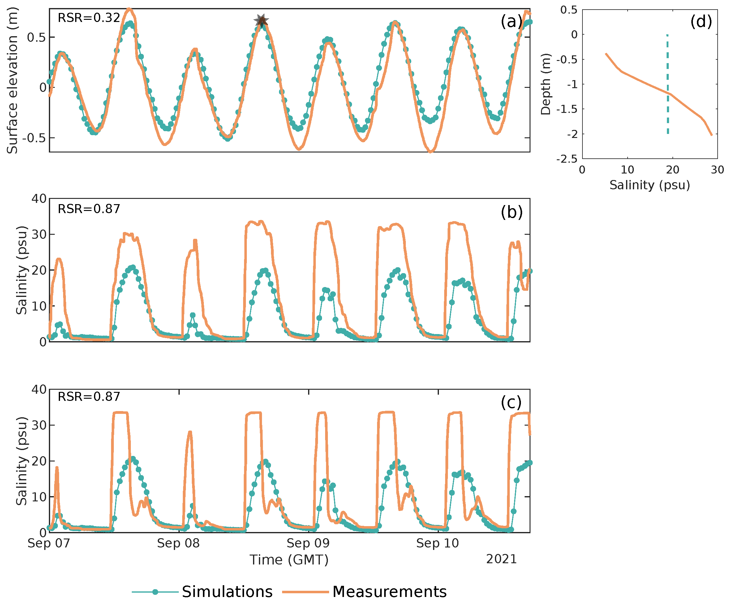
Model validation is performed by comparing a model output with CTD (conductivity–temperature–depth) measurements collected in a field campaign that took place between 7–11 September 2021 [23]. The locations of the instruments are shown in Figure 1b. A top–bottom CTD array (using YSI 600LS sensors) was placed near the river mouth, collecting data every 20 s. Additionally, another CTD (Solinst Levelogger) was deployed on a frame in the intertidal zone of the wetland and, consequently, was in and out of the water following the tides and water levels inside the estuary. This CTD was placed 14 cm from the bottom and collected data every 10 s.

For the validation process, we used a discharge equal to 12 m³s⁻¹ that was obtained from cross-sectional velocity and depth measurements (Figure 1b) collected using a Teledyne Sentinel V20 ADCP (Acoustic Doppler Current Profiler) attached to a kayak. The transects were conducted from the southwest to the northeast river banks during one ebb tide. The kayak was equipped with a Garmin ECHOMAP UHD 64cv sonar, which recorded latitude, longitude, and depth measurements over time. Finally, the river salinity was set to 0 psu, while the ocean salinity was set to 33.8 psu (measured with a handheld CTD instrument). Additionally, offshore of the computational domain, we set open boundary conditions incorporating surface elevation data obtained from tidal gauge measurements near the simulated area.

Model Performance

To assess the performance of the model, we used the ratio between the root mean square error and the standard deviation of the observations (RSR), which is defined for any variable $\theta$ as follows [56]:

$$RSR=\frac{\sqrt{{\displaystyle \sum _{i=1}^{i=n}{\left({\theta }_i^{obs}-{\theta }_i^{sim}\right)}^2}}}{\sqrt{{\displaystyle \sum _{i=1}^{i=n}{\left({\theta }_i^{obs}-{\theta }_i^{mean}\right)}^2}}},$$

(7)

where the superscripts $obs$, $sim$, and $mean$ correspond to the observed, simulated, and mean values, respectively. The RSR metric ranges from zero for optimal performance to higher positive values, which indicate large differences between the observed and simulated data.

Model output was evaluated in terms of water levels and salinity (Figure 2 and Figure 3). The model demonstrated good accuracy in reproducing the timing and magnitude of the free surface measured at the anchor location, with an RSR of 0.32 (Figure 2a). Regarding salinity, the model underestimated its maximum magnitude by approximately 10 psu. Nonetheless, it effectively captured the patterns associated with tidal forcing, particularly the timing of salt intrusion at that location (Figure 2b). However, simulations did not show the abrupt change from very high to low salinity values, such that the model was not able to capture the vertical structure at that location (Figure 2b). Salinity profiles observed in the field show that the water column was highly stratified at times, with vertical changes of approximately 30 psu in 2 m of water ((Figure 2d).

Figure 3 shows a model–data comparison in the intertidal zone. We observed good agreement for the water depth over two tidal cycles with an RSR of 0.32. However, there was a 15 cm difference in the maximum depth, which is likely attributable to differences between the real bathymetry and the bathymetry included in the model. We note that the model captures the periods when the instruments are out of the water (Figure 3a). For this, model cells with a simulated water depth of less than 0.05 were considered dry. In this region, the model represented the flood–ebb variability associated to the tides; however, there was an underestimation of approximately 15 psu at the peaks. Additionally, we observed a 1.5 h delay in the occurrence of peak values due to the rapid salinity changes observed in the field that the model cannot reproduce precisely (Figure 3b).

The underestimation of salinity and the inability of the model to represent the sharp vertical salinity gradients we observed in the field data (Figure 2b–d) may be explained by the differences between the bathymetry used in the model and the real bathymetry during the field campaign. This hypothesis is based on the findings of [57], which shows that the main factor that can reduce the salinity intrusion is the cross-sectional area, affecting more than the channel curvature or bottom friction, among other variables. To test this, we used the estuary classification proposed by [58], where estuaries are classified as well mixed, partially mixed, or highly stratified according to their river Froude number $F_R=u_R/c$ and the modified tidal Froude number $\widetilde{F_T}=u_T/c$. Both $F_R=u_R/c$ and $\widetilde{F_T}=u_T/c$ relate the three main estuarine velocity components: the river velocity $u_R=Q_R/\left(BH\right)$, the tidal velocity $u_T=0.5\eta /H\sqrt{gH}$, and the baroclinic velocity $c=\sqrt{g\beta S_{ocn}H}$ [8,31], where $Q_r$ is the river discharge; B and H are the width and depth of the estuary, respectively; $\eta$ is the tidal amplitude; g is the gravity; $\beta =7.7\times {10}^{-4}$ psu⁻¹ is the salinity expansion coefficient; and $S_{ocn}$ is the ocean salinity.

In the numerical simulations, the transversal area of the river mouth was $A=B\times H=90\times 1.5$ m² = 135 m², while the maximum tidal amplitude was $\eta =0.73$ m. We computed $F_R$ and $F_T$ and concluded that the simulations should reproduce a highly stratified estuary [58]. Figure 4 shows several combinations of possible cross-sectional areas during the field campaign; we observed that, for most cases, the Maipo estuary falls in the highly stratified region, which agrees with the field measurements (Figure 2d). These results indicate that the model’s inability to simulate vertical stratification accurately is not primarily due to differences in the bathymetry of the river mouth’s cross-sectional area between the model and the actual field conditions during measurements.

Efforts to improve performance regarding salinity simulations, including vertical resolution adjustments and vertical mixing coefficient reductions, did not yield significant improvements in our simulations. Additionally, a sensitivity analysis of stratification with respect to river discharge did not show much variation, even when discharge was as low as 2.5 m³s⁻¹. Ref. [59] documented a similar challenge in reproducing sharp vertical salinity gradients, proposing reducing the Richardson number to mitigate excessive numerical mixing. However, the proposed Richardson number adjustment conflicts with the expected physical value for a homogeneous stratified shear layer. Through multiple numerical simulations with varying grid resolutions, Ref. [59] suggested that such a Richardson number modification would become unnecessary with a higher-resolution mesh, such as the 5 m resolution used in our simulations within the estuary. Thus, we conclude that the model represented surface elevation accurately but struggled to reproduce the vertical salinity gradients in a very shallow estuarine environment. Despite this, model results show that it can still capture the tidally induced variability in the salinity cycles and produce quantitative results for the saline intrusion.

2.4. Simulated Scenarios

River discharge values for the simulation of drought scenarios were obtained based on data records provided by the Dirección General de Aguas [60] for the gauging station closest to the river mouth (Cabimbao station BNA 05748001-7) over the last 40 years. This station is located approximately 20 km upstream of the river mouth. The six simulated scenarios encompass a range of river discharges, including the minimum recorded (2.5 m³s⁻¹), the average discharge observed over the last 5 years (24 m³s⁻¹), and the ecological flow rate as defined by Chilean legislation [61] (12 m³s⁻¹).

Table 1. Flow rate and corresponding river Froude number, defined as the ratio of the river and baroclinic velocities, for each simulated case.

Case	Q m3s−1	${\mathit{F}}_{\mathit{R}}=\frac{{\mathit{u}}_{\mathit{R}}}{\mathit{c}}$
Case 1	2.5	0.03
Case 2	4	0.05
Case 3	8	0.10
Case 4	12	0.14
Case 5	16	0.19
Case 6	24	0.29

provides a summary of these scenarios.

All simulations were conducted for a 14-day period, employing identical tidal time series generated from the dominant tidal constituents in the region: $M_2$, $K_2$, and $K_1$, which were obtained from measured tidal data using the T-tide tool [62]. The numerical grid and the ocean salinity value are the same as those used in the validation case.

3. Results

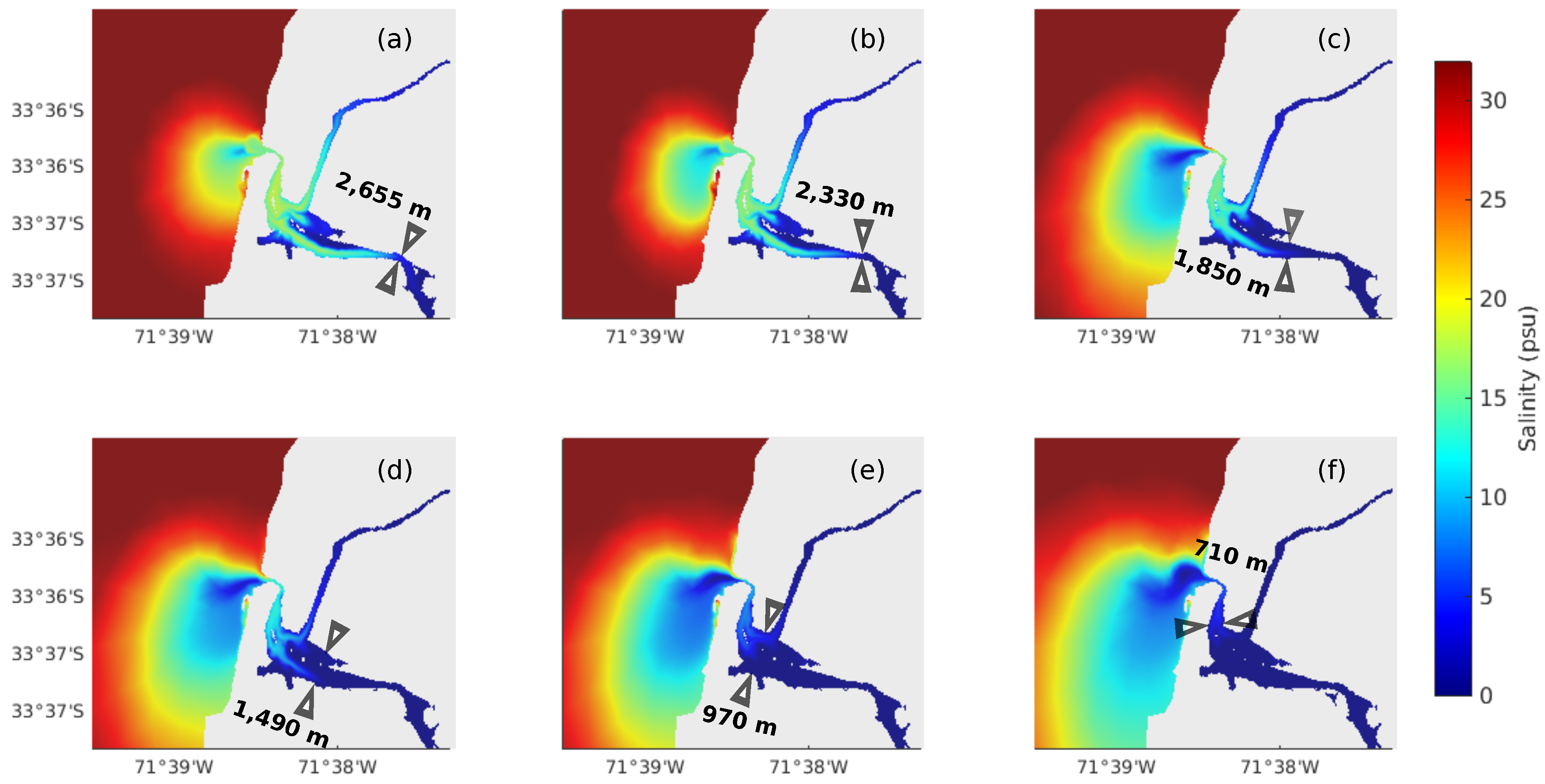
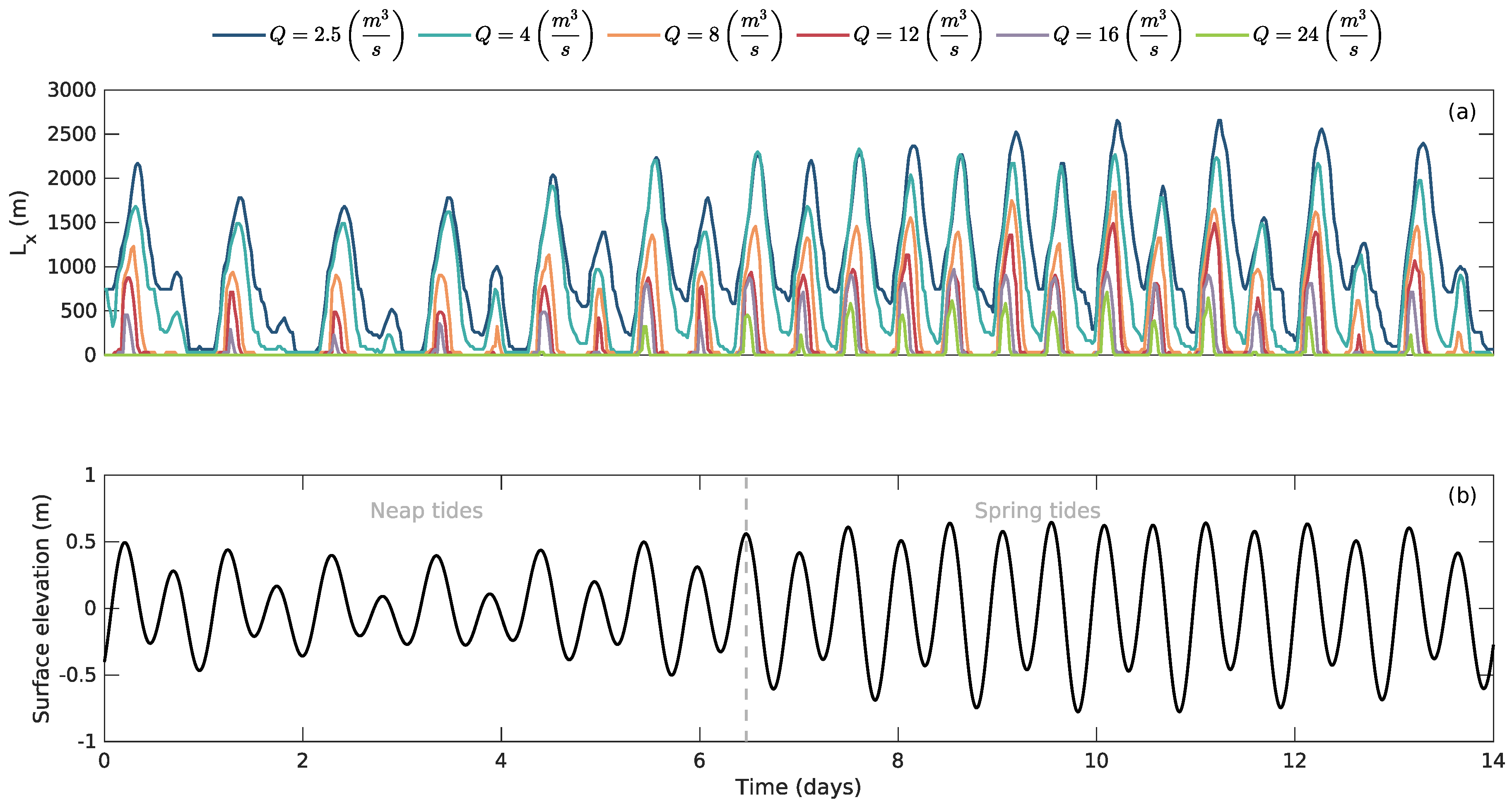
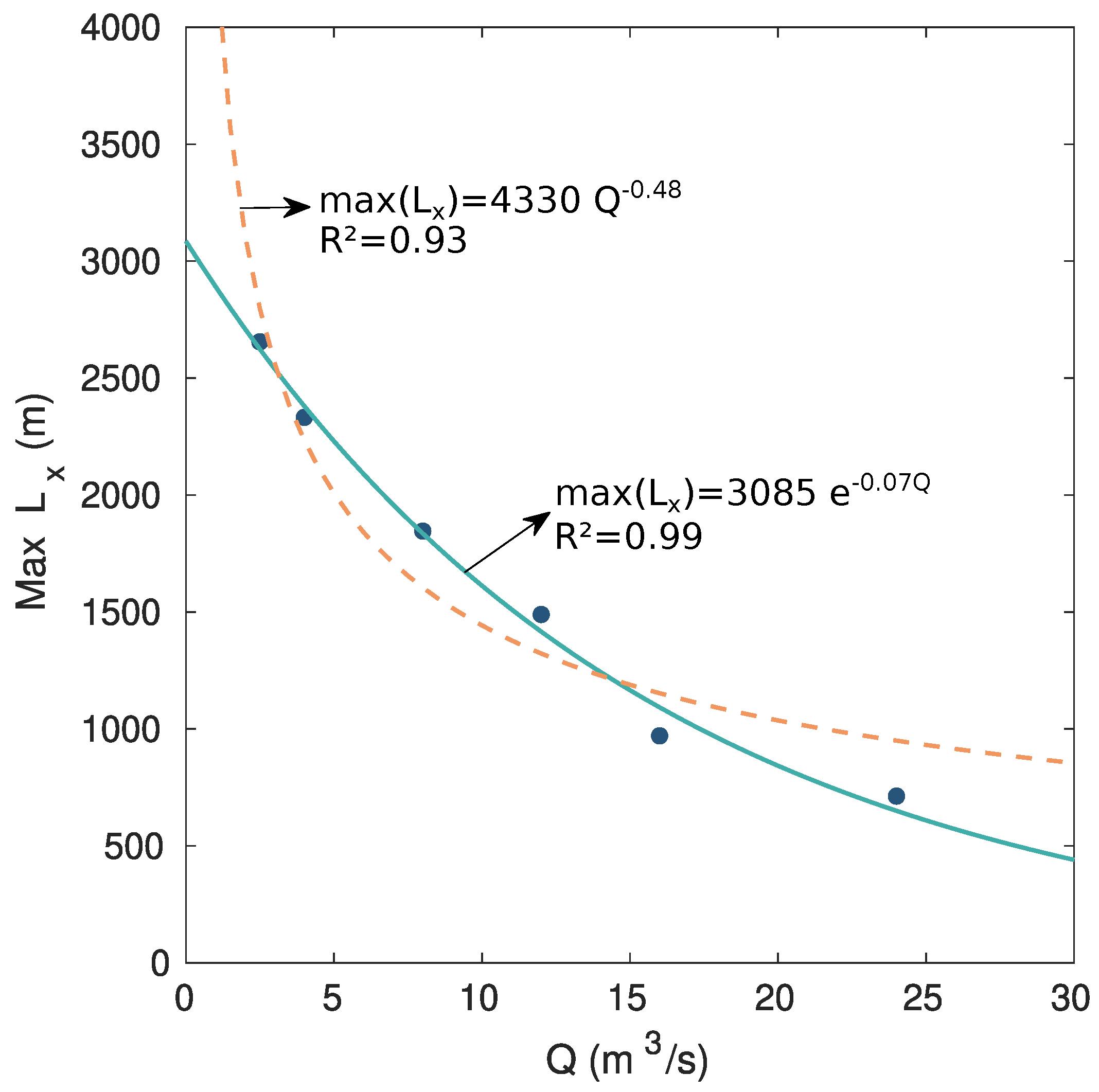
3.1. Salinity Intrusion

Figure 5 shows instantaneous bottom salinity maps at the time of the maximum intrusion for every simulated case. The maximum salinity intrusion occurs at different times, around 1 to 3 h after high tide, depending on the river discharge (Figure 6). We observe that simulations reproduce the expected effects of reducing the freshwater discharge; that is, a reduced freshwater input results in a greater salinity intrusion (e.g., [26,27,28]). The salinity intrusion is also captured in the El Sauce River, where the intrusion length can be as large as that for the Maipo River, particularly for the lowest discharge case (Figure 5a).

Figure 6 shows the salinity intrusion $L_x$, defined as the distance between the river mouth and the 2 psu isohaline, and the corresponding tidal time series. For the lowest river discharge, the salt intrusion presents variations following the mixed semidiurnal tidal regime and is also greatly affected by the condition of neap or spring tide, such that the estuary remains saline for the entire duration of the spring tide period. For the greatest river discharge simulations, we observe no saline intrusion during neap tides and only a slight increase during spring tide conditions.

In addition to analyzing the saline intrusion time series, examining the maximum intrusion concerning river discharge is crucial. Analytical studies have established a relationship of $L_x\sim Q^n$, where $n<0$ [31,32,63], with this relation being replicated in numerical simulations of larger estuarine systems (e.g., [7,8,9]).

Figure 7 presents a scatter plot of the maximum intrusion length (referenced in Figure 5) with river discharge in the Maipo River. We clearly observe a decrease in salt intrusion length with an increasing flow rate. The best-fit function reveals an exponential decay with increasing discharge, with a correlation coefficient $R^2=0.99$, which differs from the analytical expression $L_x\sim Q^n$. We note that this exponential decay has been previously observed by [64] for the three tributaries of an estuarine system in the Danshui River, Taiwan. Since our model underestimates salinity and the validation was conducted using data collected at the mouth of the estuary, the fitted function should not be used to calculate the exact length of saline intrusion; however, it offers a guide to quantitatively understanding the behavior of the estuary under drought scenarios.

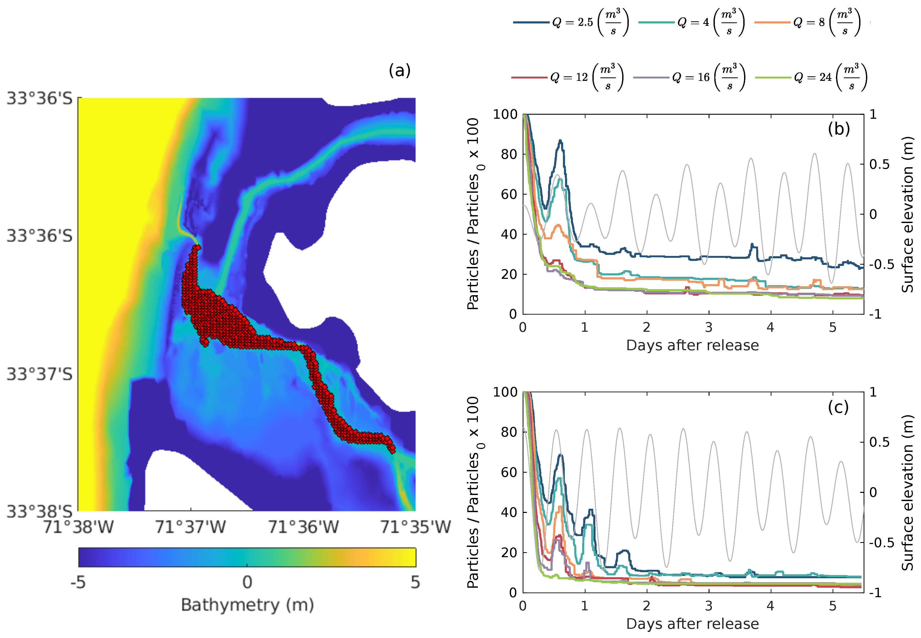
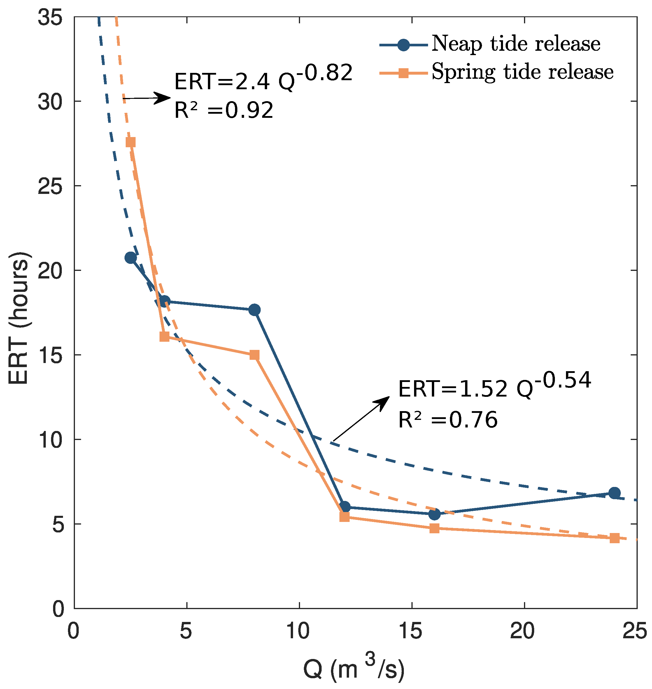
3.2. Particle Dynamics in the Estuary

Once the simulations were run, we incorporated particles in order to investigate residence times and possible convergence zones. Note that this part of the work is theoretical, as we do not compare particle dynamics results with experimental data. Here, particles are represented as passive tracers resembling the low-density microplastics (MPs). Consequently, the particles were initially distributed at the surface and spaced evenly every 50 m from the river mouth to the San Juan River, as illustrated in Figure 8a. For comparison, particles were released during both neap and spring tides during the evaluation of the impact of the tidal phase on residence times.

Figure 8b,c show the percentage of the initial number of particles remaining inside the estuary over time when released during neap and spring tides, respectively. In the neap tide scenario (Figure 8b), particles tend to re-enter the estuary during the first flood tide, which is particularly noticeable for river discharge values below 8 m³s⁻¹. Subsequently, the concentration of particles in the estuary rapidly decreases, with higher river discharge showing minimal response to surface elevation changes. In all cases, the concentration stabilizes and remains nearly constant after the first day. Conversely, particles released during spring tides (Figure 8c) tend to re-enter the estuary multiple times, which is particularly noticeable for river discharge values below 16 m³s⁻¹. During spring tides, the concentration of particles in the estuary exhibits lower values than that during the neap releases and remains nearly constant for all river discharges 2 days after the release. It is relevant to highlight that we observe lower residence times at spring tides because the tidal amplitudes are larger, reaching lower low tides that allow for more efficient flushing.

Pollutant dynamics in estuaries are usually analyzed in terms of Estuarine Residence Time (ERT), which refers to the time required for the concentration of a pollutant to reach a specified percentage of its initial value [65]. Typically, the ERT is defined using a threshold equal to 37% of the initial concentration (e.g., [65,66,67]). This threshold is calculated by modeling the concentration evolution over time, denoted as $C\left(t\right)$, using a decreasing exponential function. The function assumes that an initial concentration $C_0$ is released at time $t=0$ in an estuary of constant volume, represented mathematically as follows:

$$C\left(t\right)=C_{0}exp\left(-\frac{t}{RT}\right)$$

(8)

where $RT$ is the residence time. In Equation (8), when $t=RT$, the concentration decreases to $e^{-1}$, which corresponds to the 37% threshold mentioned earlier.

Figure 9 shows that the Estuarine Residence Time decreases as ERT $\sim Q^x$ for both neap and spring tides. This observation aligns with findings from studies such as [66,67], where pollutants begin to disperse within the estuary. However, it is important to note that the Estuarine Residence Times in those studies spanned from days to weeks, which are much higher than the ERT values found here. Additionally, Figure 9 shows an increase in residence time for higher discharges during neap tides. After careful observation, we conclude that this difference is explained by minimal differences in the paths of particles, which are influenced by the affluent branch of the El Sauce River and the complex estuarine morphology, including very shallow zones affected by wet–dry cycles.

To identify areas with the highest likelihood of retention of pollutants, referred to as hotspots, we present the time-averaged concentration, calculated as the number of particles per square meter (Figure 10). Our findings reveal consistent hotspots southeast of the El Sauce River, which remain relatively unaffected by changes in river discharge for both neap and spring release cases. This area is characterized by shallow waters and low velocity, influenced by the shear layer at the confluence. Conversely, during periods of low discharge, particles accumulate over the wetland, a shallow area that experiences continuous wet–dry cycles due to tidal level variations. Additionally, Figure 10 illustrates that hotspots become more concentrated as river discharge increases, a pattern also observed when particles are released during neap tides.

4. Discussion

In this research, we present the first approximation to drought scenarios in the Maipo River estuary, a small-scale bar built that is characteristic of river systems in central Chile and other regions with Mediterranean climates. In particular, the Maipo estuary is of significance due to the rich ecosystem it sustains [17] and the proximity to highly productive activities [18]. We used the FVCOM numerical model [47,48,49] to investigate the impacts of low river discharge on saline intrusion and the residence time of non-inertial pollutants that resemble microplastics.

The model evaluation against field observations revealed that FVCOM accurately reproduces surface elevation, with good agreement in both the phase and the amplitude within the estuary (Figure 2 and Figure 3). However, the model is not able to reproduce the vertical stratification and sharp salinity gradients that occur during flood tides [23]. We conducted a sensitivity analysis of the cross-sectional area to assess whether slight differences between the simulated domain and the field bathymetry would alter the mixing level of the estuary. This analysis involved categorizing the estuary based on the river Froude number ($F_R$) and the modified tidal Froude number ($\widetilde{F_T}$) [58]. The results suggest that the estuary is anticipated to exhibit high stratification in simulations, consistent with field observations. Therefore, this factor does not explain why the model fails to accurately reproduce the sharp vertical salinity gradient.

Previous studies have reproduced sharp vertical salinity gradients in estuaries [9,10], where [8] used FVCOM. These studies focused on wide or medium-sized estuaries, which are very different from the Maipo River estuary. An exception is found in simulations of the Cochin estuary [34], which shares similarities with the Maipo estuary in being narrow and deep and successfully replicated its salinity gradient using FVCOM. Nevertheless, a key distinction between the Cochin and Maipo estuaries lies in their depths, with Cochin exhibiting a depth one order of magnitude larger than that of the Maipo estuary. We hypothesize that the pronounced width–depth ratio ($B/H$) and the shallow characteristics of the Maipo River mouth contribute to an overestimation of mixing in the simulations. This may explain why the model struggles to represent sharp vertical salinity gradients accurately.

While the model underestimates the magnitude of salinity, it provided valuable qualitative insights into the dynamics of the Maipo River estuary. The saline intrusion time series revealed semidiurnal and fortnightly fluctuations, highlighting the significant influence of tidal variations in contrast to changes in river discharge. This suggests potentially exacerbated scenarios during storm surges [68] and future sea level rise scenarios [27,53]. However, alterations in river discharge may also significantly impact the estuary, which is particularly evident in the low discharge scenarios where extended periods with non-zero salinity were observed in the estuary. This observation aligns with the conclusions drawn in [28], which emphasizes that the salinity intrusion is influenced not just by river discharges but also by the length of drought periods. Our investigation revealed an exponential decay pattern in maximum intrusion lengths as river discharge increased (Figure 7). This finding diverges from previous studies that established a relationship between maximum intrusion and flow rate as $L_x\sim Q^n$, where $n<0$ [7,8,9,31,63], suggesting that estuaries with a high (B/H) ratio may behave differently than larger estuaries. We also recognize that the complex morphology of the Maipo River estuary may play a role in the differences we observed regarding the $L_x-Q$ relationship.

The examination of the fluxes of passive tracers indicated that river discharge has a greater impact on residence times than the tide. These tracers re-enter the estuary during drought conditions, while high discharge rates show minimal response to semi-diurnal tidal variations. Additionally, we observed differences between releasing tracers during neap and spring tides. Neap tides showed a quicker attainment of quasi-stable concentrations compared with spring tides, where the higher amplitudes facilitated particle re-entry into the estuary. However, in the releases during spring tide, the estuary reached lower concentrations than before the neap releases, indicating a faster flush of particles. We note that these simulations do not include the wave forcing, which could disperse pollutants before re-entering the estuary by generating alongshore and cross-shore coastal currents [69,70].

The Estuarine Residence Time (ERT) [65] was used to describe the retention of pollutants in the estuary. While there is no consensus for the definition of ERT, several studies define it as the time required for the concentration of a pollutant to reach 37% of its initial value (e.g., [65,66,67]). Our results show that concentration decreases as ERT $\sim Q^x$, regardless of the timing of particle release (spring or neap tides), which contrasts with the results observed for saline intrusion. This decay has been reported before, but in a wider range from days to weeks (e.g., [66,67]). Comparisons of ERTs relative to other estuarine systems are not straightforward as they hinge on factors such as initial concentration, release location, and particle characteristics [35,71]. Future studies could explore additional mathematical approaches, such as those addressing system memory in recirculating regions [72,73], to enhance particle transport descriptions. However, implementing these approaches will require a thorough analysis of the parameter space within the estuary to identify the factors governing transport time scales.

The examination of particle distributions through time-averaged concentration (Figure 10) revealed that, unlike the results reported in previous studies [12,66], there is no movement of these hotspots with increasing river discharge for both neap and spring release scenarios, likely because our simulations only consider very low freshwater discharge. Another hotspot emerged in the wetland zone, observable only at lower flow rates, where the area undergoes wet and dry cycles. As flow rates increase, hotspots become more confined, while particles disperse more widely at lower discharges, which is more noticeable when they are released at spring tides. Similar observations were made in [66] in the Tagus estuary, highlighting that the entire estuary can be considered vulnerable to pollution during low river discharges.

5. Conclusions

The outcomes of this study yield valuable insights into the dynamics of the Maipo River, which shed light on the dynamics of salinity intrusion and the accumulation of microplastics, potentially harmful factors impacting the delicate wetlands within the estuary. While the model did not fully capture the vertical structure of salinity, it provided an understanding of salinity intrusion patterns. Model results exhibit an exponential decrease in saline intrusion length with increasing river discharge. Further, our observations highlighted the predominant influence of tides on salinity intrusion, suggesting potentially exacerbated scenarios during storm surges and future sea level rise scenarios. Microplastics were represented as passive tracers and revealed a stronger reaction to river discharges than tidal cycles, with minimal differences observed between releasing them at spring and neap tides. Furthermore, severe drought conditions resulted in a more dispersed distribution of microplastics, posing challenges for accurate tracking. Overall, this research contributes to a better understanding of the response of the Maipo River estuary to low river discharge scenarios, emphasizing the need for improved modeling approaches and management strategies to address potential ecological and environmental challenges in estuarine ecosystems under changing hydrological conditions. Future research should prioritize improving the numerical model’s accuracy in representing vertical salinity gradients.

References

1. McLusky, D.S.; Elliott, M. The Estuarine Ecosystem: Ecology, Threats, and Management; Oxford University Press: Oxford, UK, 2004. [Google Scholar]
2. Day, J.W., Jr.; Kemp, W.M.; Yáñez-Arancibia, A.; Crump, B.C. Estuarine Ecology; John Wiley & Sons: Hoboken, NJ, USA, 2012. [Google Scholar]
3. Wainger, L.A.; Secor, D.H.; Gurbisz, C.; Kemp, W.M.; Glibert, P.M.; Houde, E.D.; Richkus, J.; Barber, M.C. Resilience indicators support valuation of estuarine ecosystem restoration under climate change. Ecosyst. Health Sustain. 2017, 3, e01268. [Google Scholar] [CrossRef]
4. Barbier, E.B.; Hacker, S.D.; Kennedy, C.; Koch, E.W.; Stier, A.C.; Silliman, B.R. The value of estuarine and coastal ecosystem services. Ecol. Monogr. 2011, 81, 169–193. [Google Scholar] [CrossRef]
5. Gillanders, B.M.; Elsdon, T.S.; Halliday, I.A.; Jenkins, G.P.; Robins, J.B.; Valesini, F.J. Potential effects of climate change on Australian estuaries and fish utilising estuaries: A review. Mar. Freshw. Res. 2011, 62, 1115–1131. [Google Scholar] [CrossRef]
6. Robins, P.E.; Skov, M.W.; Lewis, M.J.; Giménez, L.; Davies, A.G.; Malham, S.K.; Neill, S.P.; McDonald, J.E.; Whitton, T.A.; Jackson, S.E.; et al. Impact of climate change on UK estuaries: A review of past trends and potential projections. Estuar. Coast. Shelf Sci. 2016, 169, 119–135. [Google Scholar] [CrossRef]
7. Shaha, D.C.; Cho, Y.K.; Kim, T.W. Effects of river discharge and tide driven sea level variation on saltwater intrusion in sumjin river estuary: An application of finite-volume coastal ocean model. J. Coast. Res. 2013, 29, 460–470. [Google Scholar] [CrossRef]
8. Ralston, D.K.; Geyer, W.R.; Lerczak, J.A. Structure, variability, and salt flux in a strongly forced salt wedge estuary. J. Geophys. Res. Oceans 2010, 115. [Google Scholar] [CrossRef]
9. Ralston, D.K.; Geyer, W.R. Response to Channel Deepening of the Salinity Intrusion, Estuarine Circulation, and Stratification in an Urbanized Estuary. J. Geophys. Res. Oceans 2019, 124, 4784–4802. [Google Scholar] [CrossRef]
10. Yang, Y.; Chen, X.; Li, Y.; Xiong, M.; Shen, Z. Modeling the Effects of Extreme Drought on Pollutant Transport Processes in the Yangtze River Estuary. J. Am. Water Resour. Assoc. 2015, 51, 624–636. [Google Scholar] [CrossRef]
11. Cohen, J.H.; Internicola, A.M.; Mason, R.A.; Kukulka, T. Observations and Simulations of Microplastic Debris in a Tide, Wind, and Freshwater-Driven Estuarine Environment: The Delaware Bay. Environ. Sci. Technol. 2019, 53, 14204–14211. [Google Scholar] [CrossRef]
12. Wan, Y.; Qiu, C.; Doering, P.; Ashton, M.; Sun, D.; Coley, T. Modeling residence time with a three-dimensional hydrodynamic model: Linkage with chlorophyll a in a subtropical estuary. Ecol. Model. 2013, 268, 93–102. [Google Scholar] [CrossRef]
13. Cordero-Acosta, J.R.; Díaz, L.J.O.; Álvarez, A.E.H. Influence of Fluvial Discharges and Tides on the Salt Wedge Position of a Microtidal Estuary: Magdalena River. Water 2024, 16, 1139. [Google Scholar] [CrossRef]
14. Milliman, J.D.; Syvitski, J.P. Geomorphic/tectonic control of sediment discharge to the ocean: The importance of small mountainous rivers. J. Geol. 1992, 100, 525–544. [Google Scholar] [CrossRef]
15. McSweeney, S.; Kennedy, D.; Rutherfurd, I.; Stout, J. Intermittently Closed/Open Lakes and Lagoons: Their global distribution and boundary conditions. Geomorphology 2017, 292, 142–152. [Google Scholar] [CrossRef]
16. Izett, J.G.; Fennel, K. Estimating the cross-shelf export of riverine materials: Part 2. Estimates of global freshwater and nutrient export. Glob. Biogeochem. Cycles 2018, 32, 176–186. [Google Scholar] [CrossRef]
17. Parque humedal río Maipo. Avifauna. Available online: https://humedalriomaipo.cl/fauna-2/ (accessed on 1 June 2023).
18. Ingenieros Integrales Ltda. INFORME AMBIENTAL Modificación PRC de San Antonio Sector Portuario Sur; Technical Report; Ilustre Municipalidad de San Antonio: San Antonio, Chile, 2012. [Google Scholar]
19. Piñones, A.; Valle-Levinson, A.; Narváez, D.A.; Vargas, C.A.; Navarrete, S.A.; Yuras, G.; Castilla, J.C. Wind-induced diurnal variability in river plume motion. Estuar. Coast. Shelf Sci. 2005, 65, 513–525. [Google Scholar] [CrossRef]
20. Salcedo-Castro, J.; Saldías, G.S.; Saavedra, F.; Donoso, D. Climatology of Maipo and Rapel river plumes off Central Chile from numerical simulations. Reg. Stud. Mar. Sci. 2020, 38, 101389. [Google Scholar] [CrossRef]
21. Salcedo-Castro, J.; Olita, A.; Saavedra, F.; Saldías, G.S.; Cruz-Gómez, R.C.; Martínez, C.D.D.L.T. Modeling the interannual variability in Maipo and Rapel river plumes off central Chile. Ocean Sci. 2023, 19, 1687–1703. [Google Scholar] [CrossRef]
22. Flores, R.P.; Williams, M.E.; Horner-Devine, A.R. River Plume Modulation by Infragravity Wave Forcing. Geophys. Res. Lett. 2022, 49. [Google Scholar] [CrossRef]
23. Roco, A.; Flores, R.P.; Williams, M.E.; Saldías, G.S. Observations of river-wave interactions at a small-scale river mouth. Coast. Eng. 2024, 189, 104456. [Google Scholar] [CrossRef]
24. Garreaud, R.D.; Boisier, J.P.; Rondanelli, R.; Montecinos, A.; Sepúlveda, H.H.; Veloso-Aguila, D. The central Chile mega drought (2010–2018): A climate dynamics perspective. Int. J. Climatol. 2020, 40, 421–439. [Google Scholar] [CrossRef]
25. Dirección General de Aguas (DGA). Derechos de Aprovechamiento de Aguas Registrados en DGA. Available online: https://dga.mop.gob.cl/productosyservicios/derechos_historicos/Paginas/default.aspx (accessed on 10 January 2024).
26. Akter, R.; Asik, T.Z.; Sakib, M.; Akter, M.; Sakib, M.N.; Azad, A.S.A.; Maruf, M.; Haque, A.; Rahman, M.M. The Dominant Climate Change Event for Salinity Intrusion in the GBM Delta. Climate 2019, 7, 69. [Google Scholar] [CrossRef]
27. Pereira, H.; Sousa, M.C.; Vieira, L.R.; Morgado, F.; Dias, J.M. Modelling Salt Intrusion and Estuarine Plumes under Climate Change Scenarios in Two Transitional Ecosystems from the NW Atlantic Coast. J. Mar. Sci. Eng. 2022, 10, 262. [Google Scholar] [CrossRef]
28. Rodrigues, M.; Fortunato, A.B.; Freire, P. Saltwater intrusion in the upper tagus estuary during droughts. Geosciences 2019, 9, 400. [Google Scholar] [CrossRef]
29. Attrill, M.J.; Rundle, S.D. Ecotone or ecocline: Ecological boundaries in estuaries. Estuar. Coast. Shelf Sci. 2002, 55, 929–936. [Google Scholar] [CrossRef]
30. Tuteja, N.; Peter Singh, L.; Gill, S.S.; Gill, R.; Tuteja, R. Salinity Stress: A Major Constraint in Crop Production. In Improving Crop Resistance to Abiotic Stress; John Wiley & Sons, Ltd.: Hoboken, NJ, USA, 2012; Chapter 4; pp. 71–96. [Google Scholar] [CrossRef]
31. MacCready, P.; Geyer, W.R. Advances in estuarine physics. Annu. Rev. Mar. Sci. 2010, 2, 35–58. [Google Scholar] [CrossRef]
32. Dijkstra, Y.M.; Schuttelaars, H.M. A Unifying Approach to Subtidal Salt Intrusion Modeling in Tidal Estuaries. J. Phys. Oceanogr. 2020, 51, 147–167. [Google Scholar] [CrossRef]
33. Loose, B.; Niño, Y.; Escauriaza, C. Finite volume modeling of variable density shallow-water flow equations for a well-mixed estuary: Application to the Río Maipo estuary in central Chile. J. Hydraul. Res. 2005, 43, 339–350. [Google Scholar] [CrossRef]
34. John, S.; Muraleedharan, K.R.; Revichandran, C.; Azeez, S.A.; Seena, G.; Cazenave, P.W. What controls the flushing efficiency and particle transport pathways in a tropical Estuary? Cochin Estuary, Southwest coast of India. Water 2020, 12, 908. [Google Scholar] [CrossRef]
35. Hewageegana, V.H.; Olabarrieta, M.; Gonzalez-Ondina, J.M. Main Physical Processes Affecting the Residence Times of a Micro-Tidal Estuary. J. Mar. Sci. Eng. 2023, 11, 1333. [Google Scholar] [CrossRef]
36. Frias, J.; Nash, R. Microplastics: Finding a consensus on the definition. Mar. Pollut. Bull. 2019, 138, 145–147. [Google Scholar] [CrossRef]
37. Honorato-Zimmer, D.; Kiessling, T.; Gatta-Rosemary, M.; Kroeger Campodónico, C.; Núñez-Farías, P.; Rech, S.; Thiel, M. Mountain streams flushing litter to the sea – Andean rivers as conduits for plastic pollution. Environ. Pollut. 2021, 291, 118166. [Google Scholar] [CrossRef] [PubMed]
38. Harris, P.T. The fate of microplastic in marine sedimentary environments: A review and synthesis. Mar. Pollut. Bull. 2020, 158, 111398. [Google Scholar] [CrossRef] [PubMed]
39. Setälä, O.; Fleming-Lehtinen, V.; Lehtiniemi, M. Ingestion and transfer of microplastics in the planktonic food web. Environ. Pollut. 2014, 185, 77–83. [Google Scholar] [CrossRef] [PubMed]
40. Nerland, I.L.; Halsband, C.; Allan, I.; Thomas, K.V. Microplastics in Marine Environments: Occurrence, Distribution and Effects; Technical Report; Norwegian Institute for Water Research: Oslo, Norway, 2014. [Google Scholar]
41. Sharma, S.; Chatterjee, S. Microplastic pollution, a threat to marine ecosystem and human health: A short review. Environ. Sci. Pollut. Res. 2017, 24, 21530–21547. [Google Scholar] [CrossRef] [PubMed]
42. Wendt, J.F. Computational Fluid Dynamics: An Introduction; Springer: Berlin/Heidelberg, Germany, 2008. [Google Scholar]
43. Kundu, P.K.; Cohen, I.M.; Dowling, D.R. Fluid Mechanics; Academic Press: Cambridge, MA, USA, 2015. [Google Scholar]
44. Zawawi, M.H.; Saleha, A.; Salwa, A.; Hassan, N.H.; Zahari, N.M.; Ramli, M.Z.; Muda, Z.C. A review: Fundamentals of computational fluid dynamics (CFD). AIP Conf. Proc. 2018, 2030, 020252. [Google Scholar] [CrossRef]
45. Schulz, E.; Schuttelaars, H.M.; Gräwe, U.; Burchard, H. Impact of the depth-to-width ratio of periodically stratified tidal channels on the estuarine circulation. J. Phys. Oceanogr. 2015, 45, 2048–2069. [Google Scholar] [CrossRef]
46. Alahmed, S.; Ross, L.; Smith, S.M. Coastal Hydrodynamics and Timescales in Meso-Macrotidal Estuaries in the Gulf of Maine: A Model Study. Estuaries Coasts 2022, 45, 1888–1908. [Google Scholar] [CrossRef]
47. Chen, C.; Liu, H.; Beardsley, R.C. An Unstructured Grid, Finite-Volume, Three-Dimensional, Primitive Equations Ocean Model: Application to Coastal Ocean and Estuaries. J. Atmos. Ocean. Technol. 2003, 20, 159–186. [Google Scholar] [CrossRef]
48. Chen, C.; Beardsley, R.; Cowles, G. An unstructured grid, finite-volume coastal ocean model (FVCOM) system. Oceanography 2006, 19, 78–89. [Google Scholar] [CrossRef]
49. Huang, H.; Chen, C.; Cowles, G.W.; Winant, C.D.; Beardsley, R.C.; Hedstrom, K.S.; Haidvogel, D.B. FVCOM validation experiments: Comparisons with ROMS for three idealized barotropic test problems. J. Geophys. Res. Ocean. 2008, 113, 1–14. [Google Scholar] [CrossRef]
50. Chen, C.; Qi, J.; Li, C.; Beardsley, R.C.; Lin, H.; Walker, R.; Gates, K. Complexity of the flooding/drying process in an estuarine tidal-creek salt-marsh system: An application of FVCOM. J. Geophys. Res. Ocean. 2008, 113. [Google Scholar] [CrossRef]
51. Li, C.; Huang, W.; Milan, B. Atmospheric cold front-induced exchange flows through a microtidal multi-inlet bay: Analysis using multiple horizontal ADCPs and FVCOM simulations. J. Atmos. Ocean. Technol. 2019, 36, 443–472. [Google Scholar] [CrossRef]
52. Xiao, Z.; Yang, Z.; Wang, T.; Sun, N.; Wigmosta, M.; Judi, D. Characterizing the Non-linear Interactions Between Tide, Storm Surge, and River Flow in the Delaware Bay Estuary, United States. Front. Mar. Sci. 2021, 8, 715557. [Google Scholar] [CrossRef]
53. Liu, J.; Hetland, R.D.; Yang, Z.; Wang, T.; Sun, N. Response of Salt Intrusion in a Tidal Estuary to Regional Climatic Forcing (FVCOM Output for the baseline scenario). 2024. [Google Scholar] [CrossRef]
54. Zhao, C.; Wang, N.; Ding, Y.; Song, D.; Li, J.; Li, M.; Zhou, L.; Yu, H.; Chen, Y.; Bao, X. Numerical Study on the Formation Mechanism of Plume Bulge in the Pearl River Estuary under the Influence of River Discharge. Water 2024, 16, 1296. [Google Scholar] [CrossRef]
55. Rodi, W. Turbulence Models and Their Application in Hydraulics; Routledge: London, UK, 2000. [Google Scholar] [CrossRef]
56. Moriasi, D.N.; Arnold, J.G.; Van Liew, M.W.; Bingner, R.L.; Harmel, R.D.; Veith, T.L. Model evaluation guidelines for systematic quantification of accuracy in watershed simulations. Trans. ASABE 2007, 50, 885–900. [Google Scholar] [CrossRef]
57. Hendrickx, G.G.; Kranenburg, W.M.; Antolínez, J.A.; Huismans, Y.; Aarninkhof, S.G.; Herman, P.M. Sensitivity of salt intrusion to estuary-scale changes: A systematic modelling study towards nature-based mitigation measures. Estuar. Coast. Shelf Sci. 2023, 295, 108564. [Google Scholar] [CrossRef]
58. Guha, A.; Lawrence, G.A. Estuary classification revisited. J. Phys. Oceanogr. 2013, 43, 1566–1571. [Google Scholar] [CrossRef]
59. Ralston, D.K.; Cowles, G.W.; Geyer, W.R.; Holleman, R.C. Turbulent and numerical mixing in a salt wedge estuary: Dependence on grid resolution, bottom roughness, and turbulence closure. J. Geophys. Res. Ocean. 2017, 122, 692–712. [Google Scholar] [CrossRef]
60. Dirección General de Aguas (DGA). Información Oficial Hidrometeorológica y de Calidad de Aguas en Línea. Available online: https://snia.mop.gob.cl/BNAConsultas/reportes (accessed on 15 August 2023).
61. Biblioteca Nacional del Congreso de Chile. Criterios para la Determinación del Caudal Ecológico Mínimo para el Otorgamiento de Derechos de Aprovechamiento de Aguas. 2015. Available online: https://www.bcn.cl/leychile/navegar?idNorma=1053200 (accessed on 15 September 2023).
62. Pawlowicz, R.; Beardsley, B.; Lentz, S. Classical tidal harmonic analysis including error estimates in MATLAB using T-TIDE. Comput. Geosci. 2002, 28, 929–937. [Google Scholar] [CrossRef]
63. Monismith, S.G.; Burau, J.R.; Stacey, M.T. Structure and Flow-Induced Variability of the Subtidal Salinity Field in Northern San Francisco Bay. J. Phys. Oceanogr. 2002, 32, 3003–3019. [Google Scholar] [CrossRef]
64. Liu, W.C.; Ke, M.H.; Liu, H.M. Response of salt transport and residence time to geomorphologic changes in an estuarine system. Water 2020, 12, 1091. [Google Scholar] [CrossRef]
65. Miller, R.L.; McPherson, B.F. Estimating estuarine flushing and residence times in Charlotte Harbor, Florida. via salt balance and a box model. Limnol. Oceanogr. 1991, 36, 602–612. [Google Scholar] [CrossRef]
66. de Pablo, H.; Sobrinho, J.; Garaboa-Paz, D.; Fonteles, C.; Neves, R.; Gaspar, M.B. The Influence of the River Discharge on Residence Time, Exposure Time and Integrated Water Fractions for the Tagus Estuary (Portugal). Front. Mar. Sci. 2022, 8, 734814. [Google Scholar] [CrossRef]
67. Huang, W.; Liu, X.; Chen, X.; Flannery, M.S. Critical Flow for Water Management in a Shallow Tidal River Based on Estuarine Residence Time. Water Resour. Manag. 2011, 25, 2367–2385. [Google Scholar] [CrossRef]
68. Kranenburg, W.M.; Kaaij, T.V.D.; Tiessen, M.; Friocourt, Y.; Blaas, M. Salt Intrusion in the Rhine Meuse Delta: Estuarine Circulation, Tidal Dispersion or Surge Effect? In Proceedings of the 39th IAHR World Congress, Granada, Spain, 19–24 June 2022. [Google Scholar] [CrossRef]
69. Longuet-Higgins, M.S. Longshore currents generated by obliquely incident sea waves: 1. J. Geophys. Res. 1970, 75, 6778–6789. [Google Scholar] [CrossRef]
70. Pezerat, M.; Bertin, X.; Martins, K.; Lavaud, L. Cross-shore distribution of the wave-induced circulation over a dissipative beach under storm wave conditions. J. Geophys. Res. Ocean. 2022, 127, e2021JC018108. [Google Scholar] [CrossRef]
71. Pawlowicz, R.; Hannah, C.; Rosenberger, A. Lagrangian observations of estuarine residence times, dispersion, and trapping in the Salish Sea. Estuar. Coast. Shelf Sci. 2019, 225. [Google Scholar] [CrossRef]
72. Sandoval, J.; Mignot, E.; Mao, L.; Pastén, P.; Bolster, D.; Escauriaza, C. Field and numerical investigation of transport mechanisms in a surface storage zone. J. Geophys. Res. Earth Surf. 2019, 124, 938–959. [Google Scholar] [CrossRef]
73. Barros, M.; Escauriaza, C. Lagrangian and Eulerian perspectives of turbulent transport mechanisms in a lateral cavity. J. Fluid Mech. 2024, 984, A1. [Google Scholar] [CrossRef]
Figure 1. (a) Computational domain used for all simulations. (b) Zoomed-in area within the computational domain, highlighting the location of the instrument during the field campaign.
Jmse 12 01162 g001
Figure 2. Comparison of measurements and numerical simulation results in the anchor zone: (a) surface elevation; (b,c) salinity at the bottom and top channels, respectively; and (d) vertical salinity profile measured during high tides highlighted in (a).
Jmse 12 01162 g002
Figure 3. Comparison between measurements and numerical simulation results in the frame zone: (a) depth time series and (b) salinity at a depth of 14 cm from the bottom.
Jmse 12 01162 g003
Figure 4. River Froude number, F R , and modified tidal Froude number, F T ˜ , calculated with the field campaign conditions and using different transversal areas ( A = B × H ). The black dashed line corresponds to the division between partially mixed and highly stratified estuary proposed by [58].
Jmse 12 01162 g004
Figure 5. Screenshot of maximum bottom salinity intrusion for all simulated flow rates. Triangles indicate the distance measured from the river mouth along the main streamline upstream up to the 2 psu isohaline. (a) Q = 2.5 m3s−1, (b) Q = 4 m3s−1, (c) Q = 8 m3s−1, (d) Q = 12 m3s−1, (e) Q = 16 m3s−1, (f) Q = 24 m3s−1.
Jmse 12 01162 g005
Figure 6. (a) Length of saline intrusion L x in the Maipo River, calculated as the distance from the river mouth through the main streamline up to the 2 psu isohaline for all the simulated flow rates. (b) Surface elevation time series indicates neap and spring tides.
Jmse 12 01162 g006
Figure 7. Maximum saline intrusion length L x depicted with simulated results as dots. The continuous line represents the best-fit function, while the dashed line represents the fit function based on the classical theory L x Q n .
Jmse 12 01162 g007
Figure 8. (a) Initial position of passive particles evenly distributed at the surface every 50 m. (b,c) The percentage of remaining particles inside the estuary for neap and spring releases, respectively; the gray line indicates the tidal surface elevation.
Jmse 12 01162 g008
Figure 9. Estuarine Residence Time (ERT), calculated as the time required for the concentration to decrease to 37% of its initial value. For simplicity, this figure marks when the concentration reaches this threshold and does not rise again. Dashed lines indicate the best-fit curve for each release case.
Jmse 12 01162 g009
Figure 10. Mean concentration over time, calculated as the averaged number of particles per square meter. (a) Q = 2.5 m3s−1, (b) Q = 4 m3s−1, (c) Q = 8 m3s−1, (d) Q = 12 m3s−1, (e) Q = 16 m3s−1, and (f) Q = 24 m3s−1, for the neap release case (.1) and the spring release case (.2).
Jmse 12 01162 g010