Abstract
The difference between waterway traffic and road traffic in terms of lane lines leads to the direct application of the method of plotting the fundamental diagram of road traffic flow to waterway traffic, and it is difficult to reveal the mechanism of waterway traffic flow operations. This study proposes a shipping-lane-subdivision approach to tackle this problem. Additionally, it introduces a more suitable fundamental diagram-plotting method for waterway traffic based on the aforementioned method. The southern channel in the estuary of the Yangtze River was taken as the research water, and the fundamental diagram of traffic flow in this water was plotted to verify the similarities between the fundamental diagram of waterway traffic flow and the fundamental diagram of road traffic flow. Upon evaluating the plotted fundamental diagram, it was determined that the blockage density of the subdivided shipping lane is around 6.5 vessels per nautical mile. This method has significant potential for its application in the theory of waterway traffic flow.
1. Introduction
The fundamental diagram of waterway traffic flow is a central component of the theory of waterway traffic flow. It serves as a vital tool for waterway traffic workers to assess congestion levels and determine the capacity of the waterway [1]. Waterway management departments can utilize key parameters such as optimal speed, optimal density, and congestion density to effectively manage vessel operations in waterways. This enables them to ensure the safety of vessels while enhancing navigation efficiency. Additionally, the fundamental diagram of waterway traffic flow serves as a theoretical and data-driven tool for waterway planning departments, providing valuable support in the planning process [2]. Given the gravity of issues such as waterway traffic congestion and low passage efficiency, scholars are increasingly recognizing the value of fundamental diagrams of waterway traffic flow as a significant tool for proposing efficient solutions to ameliorate waterway traffic challenges [3,4,5,6].
The theory of road traffic flow was initially proposed and developed within the field of road transportation, with distinctive characteristics of road transportation [1,7]. The procedure of this method primarily entails the selection of lanes to be examined, gathering vehicle data, constructing the spatio-temporal trajectory diagram of vehicles, computing traffic flow characteristics based on the spatio-temporal trajectory diagram, and plotting the fundamental diagram [8]. The determination of road traffic flow characteristics typically relies on the spatio-temporal trajectory diagram of cars on a single lane, which excludes any data related to overtaking or parallel vehicle trajectories [9]. This not only facilitates the exploration of the relationship between headway and vehicle speed in road traffic but also renders the detection of traffic congestion waves in road traffic relatively effortless [10]. The construction of the fundamental diagram of waterway traffic flow also utilizes this approach. Unlike road traffic, waterway traffic does not have lane lines. If the study area is regarded as a lane and not subdivided into shipping lanes when plotting the fundamental diagram, the ship spatial–temporal trajectory diagram will show overtaking or parallel vehicle trajectory data [11]. It not only interferes with the calculation of the traffic flow characteristics but is also not conducive to exploring the binary relationship between waterway traffic flow characteristics.
This study aims to investigate how to plot the fundamental diagram of waterway traffic flow. On the basis of the waterway division method proposed in this article, a plotting method of the fundamental diagram of waterway traffic flow that is more in line with the characteristics of waterway traffic is proposed, and the fundamental diagram of waterway traffic flow is analyzed. Section 2 provides a concise overview of this study pertaining to the fundamental diagram of waterway traffic flow. Section 3 introduces the process of constructing the fundamental diagram of waterway traffic flow, the method of the Automatic Identification System (AIS) data processing, the method of subdividing shipping lanes, and the calculation of traffic flow characteristics. These methods will be used to plot the fundamental diagram of waterway traffic flow. In Section 4, the southern channel in the estuary of the Yangtze River is taken as the research object. Based on AIS data and the method proposed in this paper for plotting the fundamental diagram of waterway traffic flow, the fundamental diagram of waterway traffic flow was analyzed. Finally, conclusions and future studies are summarized in Section 5.
2. Literature Review
The notion of the fundamental diagram of traffic was initially introduced in the 1930s [12]. The fundamental diagram of traffic flow is a graphical representation of the correlation between flow, speed, and density. It serves as a valuable tool for interpreting traffic operations and investigating traffic issues from a macroscopic perspective. The fundamental diagram of traffic is extensively utilized in various transportation modes, including road traffic, pedestrian traffic, railroad traffic, and so on [13,14,15,16].
As shown in Table 1, Greenshields (GD) et al. [12] initially explored the continuous traffic flow of a single lane and were the first to develop the fundamental relationship model of traffic flow. They proposed this model, which is also known as the equilibrium state model of the fundamental diagram of traffic flow. Subsequently, other scholars have proposed some improved models based on the fundamental diagram of traffic flow proposed by GD [17,18]. In 1996, Cassidy et al. [19] conducted a study on the fundamental diagram of multi-lane traffic flow composed of multiple single lanes. The research findings show the existence of a distinct binary relationship between the traffic flow characteristics of a multi-lane traffic flow composed of multiple single lanes. In road traffic, the lanes on the road are usually delineated by clear physical lane lines, so that vehicles operate with strict lane discipline. These scholars, in the process of plotting the fundamental diagram of road traffic flow based on an individual lane, are largely free from the data of pursuit and parallelism in the diagram of spatio-temporal trajectories of vehicles. This makes the fundamental diagram become a tool for revealing the variation law between headway and vehicle speed in road traffic and also makes the macroscopic form of the fundamental diagram of traffic flow closely related to the following microscopic behavior. Some scholars have utilized this relationship to derive fundamental diagram models from microscopic car-following models, and these models have shown good results in fitting empirical data [10,20,21]. Furthermore, in 2021, Ni [22] conducted an analysis and explanation of some phenomena in the fundamental diagram of traffic flow using a car-following model from a microscopic perspective. This proves the feasibility of using microscopic car-following models to derive the macroscopic representation of traffic flow, which in turn reveals the traffic flow phenomenon and the mechanism of traffic flow evolution. With the development of automatic driving technology in recent years, the fundamental diagram of traffic also has a wide range of applications in related fields as well. For example, Xiaowei Shi et al. [23] proposed a general methodology that combines both empirical experiments and theoretical models to construct a fundamental diagram of mixed traffic flow to investigate the impacts of commercial automatic vehicles on traffic flow. This methodology can serve as a methodological foundation for studying future mixed traffic flow features with uncertain and evolving automatic-vehicle technologies.

Table 1.
Comparison of traffic flow fundamental diagrams.
As the fundamental diagram of road traffic flow has been developed and improved, scholars have started applying the theories and plotting methods of the fundamental diagram of road traffic flow to waterways for solving related problems in waterway transportation. In 2017, Tasseda et al. [3] mined and analyzed the AIS data of ships in the waters of Tokyo Bay through big data technology, uncovered the correlation between marine traffic flow characteristics in this region, and identified certain resemblances with road traffic flow patterns. Qi et al. [4] and Feng et al. [6] built a waterway traffic flow model based on cellular automata to study these phenomena. From the fundamental diagram, the relationship between traffic ability and the lengths of ships was explored. However, since these fundamental diagrams were based on simulation data, they did not reflect the real traffic situation in the waters. Kang et al. [24], by mining the historical AIS data of the Singapore Strait, proposed a fundamental diagram model of marine traffic flow based on the fundamental diagram of road traffic flow and estimated the theoretical capacity of the strait. They pointed out that the proposed fundamental diagram model of traffic flow considered ship-following behaviors and did not take into account overtaking behaviors. Huang et al. [2] estimated the three primary variables of fundamental diagrams. The relationships among three variables were discussed, and marine traffic data were further compared and contrasted with classical traffic flow models. The results show that the marine traffic flow is very similar to the road traffic flow, but they do not fully conform to any existing known fundamental relationship. Huang et al. pointed out that the absence of actual lane-splitting boundaries for ship traffic may lead to discrepancies between the fundamental diagram model of traffic flow and empirical data. When scholars plot fundamental diagrams of waterway traffic flow, they usually adopt the method of plotting the fundamental diagrams of road traffic flow directly, and scholars usually regard the whole study area as a shipping lane [2,3,5,11,24]. This method has the following disadvantages:
Firstly, this method leads to a large number of ship overtaking and paralleling data in the ship spatio-temporal trajectory diagrams, which not only interferes with the calculation of traffic flow features but also affects the study of the relationship between traffic flow characteristics. Secondly, traffic waves are not easily found in the ship spatio-temporal trajectory diagram due to the influence of trajectory overlaps and crossovers. Third, affected by a large amount of non-ship-following data, treating the whole study area as a shipping lane not only facilitates the investigation of the relationship between the headway and speed in waterway traffic but also makes it difficult to validate the fundamental diagrams of traffic flow derived by using the microscopic ship-following model with these spatio-temporal data.
In summary, due to the differences in lane lines between road traffic and waterway traffic, if the study area is considered as one shipping lane and not subdivided into shipping lanes when plotting the fundamental diagrams of waterway traffic flow, this may affect the calculation of waterway traffic flow characteristics and the presentation of the fundamental diagrams of waterway traffic flow, which is not conducive to the analysis of the relationship between the waterway traffic flow characteristics and the investigation of the mechanism of the operation of waterway traffic flow. How to divide shipping lanes and extract the traffic data in shipping lanes to plot fundamental diagrams has become an important problem to be solved, but there are few research studies in this area at present.
3. Methodology
This study required the preprocessing of AIS data in order to implement the plotting process and method of the fundamental diagram of waterway traffic flow suggested in this paper. As shown in Figure 1, the preprocessing of AIS data consists of three steps: filtering the AIS data of the waterways, establishing the channel coordinate system, and converting the latitude and longitude coordinates.
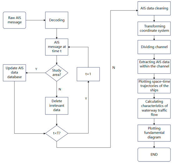
Figure 1.
A method for plotting fundamental diagrams of waterway traffic flow based on ship AIS data.
- (1)
- Screening of AIS data in the designated study area: to obtain the AIS data from the research waters, it is imperative to decipher the unprocessed data in the AIS database of the designated study area and, thereafter, conduct a screening process.
- (2)
- Cleaning the AIS data;
- (3)
- Coordinate system conversion;
- (4)
- Subdividing shipping lanes;
- (5)
- Calculating characteristics of waterway traffic flow;
- (6)
- Plotting the fundamental diagram of waterway traffic flow.
In the present state of studying the fundamental diagram of waterway traffic flow, the procedure for plotting the fundamental diagram can be broadly categorized into the following stages: analyzing the AIS data of the waters to be studied, establishing the coordinate system of the waterway, converting the latitude and longitude coordinates, plotting the spatio-temporal trajectory of the ships, calculating traffic flow characteristics, and generating the fundamental diagram. This approach to plotting the fundamental diagram treats the study area as a lane. Typically, while studying the fundamental diagram of road traffic flow, researchers choose either a single-lane or a multi-lane road consisting of multiple single lanes as the focus of their investigation. Hence, the research methodology that treats the entire study area as a shipping lane fails to acknowledge the distinction between waterway traffic and road traffic, necessitating the division of the channel. This study improves the current method of plotting the fundamental diagram of waterway traffic flow by incorporating the process of subdividing shipping lanes. This modification would better represent the practicalities of aquatic transportation.
3.1. Coordinate System Conversion
To facilitate the plotting of space–time trajectories of ships, it is advantageous to convert the latitude and longitude information in the AIS data into Cartesian coordinate data. Create a Cartesian coordinate system for the chosen fairway. The precise procedure is as follows.
The data coordinate is taken as the origin of the Cartesian coordinate system of the waterway, and the latitude and longitude coordinates of the AIS data in the waterway database are converted into the vertical coordinates (X value) and horizontal coordinates (Y value) in the Cartesian coordinate system. Among them, the X value indicates the longitudinal distance of the ship from the reference point, and the Y value indicates the transverse distance of the ship from the data coordinate. The Cartesian coordinate system used for the channel is depicted in Figure 2.
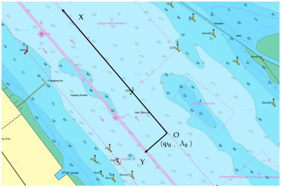
Figure 2.
Schematic of the Cartesian coordinate system used for the channel.
Through the Mercator projection method and the trigonometric relationship, the position of the AIS data points in the Cartesian coordinate system of the channel can be calculated. Figure 3 displays the schematic diagram illustrating the process for transforming latitude and longitude coordinates into Cartesian coordinates.
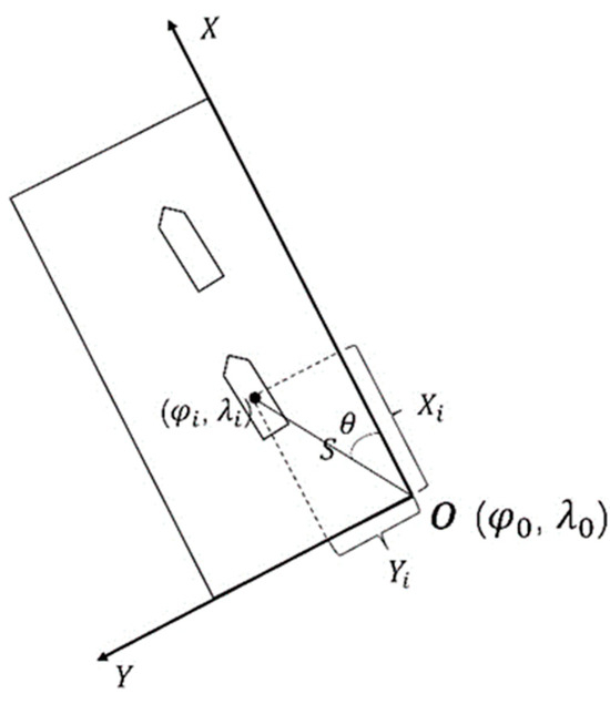
Figure 3.
Sketch of the process for transforming latitude and longitude coordinates into Cartesian coordinates.
This process is as follows:
Mark the latitude and longitude coordinates of the datum coordinate as (, ) and the latitude and longitude coordinates of the ship’s AIS data point in the channel as (, ), and utilize the Mercator projection method to calculate the voyage. The relevant calculation formula is as follows:
where S is the voyage, is the latitude difference, is the longitude difference, is the meridional curvature where the AIS data point is located, is the meridional curvature where the data point is located, is the difference of meridional curvature, is the course, is the angle between the data coordinate and the straight line connecting the AIS data point and the direction of the channel, is the value corresponding to the AIS data point in the coordinate system of the channel, and is the value corresponding to the AIS data point in the coordinate system of the channel.
3.2. Methods of Subdividing Shipping Lanes
When it comes to plotting the fundamental diagram of waterway traffic flow that represents the relationships among the flow, speed, and density of waterway traffic flow characteristics, very few researchers have put forward any viable strategies for accurately defining the boundaries of the waterway. This study presents the novel approach of subdividing shipping lanes.
The Ship Safety Domain is the area that is maintained to avoid collisions, a zone maintained in the fore and aft of each ship that is not violated by other ships [25]. The Ship Safety Domain has evolved to be recognized by maritime and shipping-related authorities and practitioners as an important basis for assessing the navigation status of ships in restricted waters and risks in the waterway. Considering that the dimensions of a ship domain are usually measured in terms of the length of a standard ship or the average length of ships, it is customary for pilots to keep the distance between ships in multiples of the ship’s length, such as 0.5 times the length of the ship or 1 times the length of the ship, to ensure that the ships are safe from each other [26]. Using this feature, the novel approach of subdividing shipping lanes is proposed as shown in Figure 4 and Algorithm 1. The processes are as outlined below:

Figure 4.
Schematic diagrams of the method of subdividing shipping lanes.
The data processing method was employed to calculate the mean length, mean width, and initial transverse position of vessels upon entering the channel using the AIS data of the channel first. Then, based on these data, the width of the waterway was divided by 0.5 times the average length of the ship for each subdivision. The subdivided shipping lane was then shifted by 1 times the average width of the ship. The number of AIS ship track points within each individual shipping lane was recorded and calculated as a percentage of the total number of AIS ship track points in the study area. The appropriate width of shipping lanes and the most suitable shipping lanes for producing the fundamental diagram of waterway traffic flow were determined based on the ratio.
To minimize the impact of ship overtaking on the calculation of traffic flow characteristics, it is vital to ensure that the width of the subdivided shipping lane is not excessively big. The optimal width of the subdivided shipping lane was determined by analyzing examples and identifying the width at which the proportion of trajectory points in the segment data exceeds a preset threshold. The data within this interval were then used as the basis for processing ship traffic flow. In this study, the threshold value set to characterize the traffic flow of the subdivided shipping lane is 85%, following the common practice of threshold setting and data statistics in transportation research.
To determine whether an AIS data point is in the corresponding subdivided shipping lane, the relationship between the lateral position Y of the AIS data point in the channel coordinate system (), the length of the channel , and the lateral position Y at the midpoint of the subdivided shipping lane () can be used to judge the AIS data point’s distance away from the midline of the subdivided channel, which is taken as :
If is satisfied, the AIS data point can be judged to be within the subdivided shipping lane; conversely, the data point deviates from the subdivided shipping lane.
When using the fundamental diagram for calculating the capacity of the channel, the capacity derived from this subdivided shipping lane data can be used as the capacity for each subdivided shipping lane, i.e., the capacity of this researched waterway is the product of the subdivided shipping lane capacity and the number of subdivided shipping lanes.
| Algorithm 1: Dividing Channel—Pseudo-code for subdividing shipping lane method | |
| Input: | Vessel length, vessel width, vessel spherical coordinates, positional information of study waters |
| Output: | Location of right and left shipping lane boundaries, shipping lane width |
| 1 | Average ship length = total length of all ships/total number of ships |
| 2 | Average ship width = total width of all ships/total number of ships |
| 3 | Ship’s planar coordinates = ship’s spherical coordinates * matrix of coordinate changes |
| 4 | Total number of ship trajectory points = number of ship trajectory points in the statistical study area |
| 5 | Yleft bound = 0; = average ship’s length; B = average ship’s breadth; Yright bound = width of study waters |
| 6 | Shipping lane_i (left bound, right bound) = (Yleft bound, Yleft bound + ] |
| 7 | Aisdata = extracting AIS data within the shipping lane_i |
| 8 | Number of ship trajectory points in Shipping lane_i = statistics of ship trajectory points through Aisdata |
| 9 | If number of ship trajectory points in Shipping lane_i/total number of ship track points is ≥ threshold a: Return Shipping lane_i End Else: Shipping lane_i (left bound, right bound] = (left bound + B, right bound + B] If right bound +B ≤ Yright bound Continue (7) |
| 10 | If Shipping lane_i is none: Shipping lane_i (left bound, right bound) = (Yleft bound, Yleft bound + 1.5 ] Continue (7) |
| 11 | If Shipping lane_i is none: Shipping lane_i (left bound, right bound) = (Yleft bound, Yleft bound + 2 ] Continue (7) |
| 12 | If Shipping lane_i is none: Shipping lane_i (left bound, right bound) = (Yleft bound, Yleft bound + 2.5 ] Continue (7) |
| 13 | End |
3.3. Calculating Characteristics of Waterway Traffic Flow
To analyze the fundamental diagram of traffic flow, it is necessary to first establish the defining characteristics of waterway traffic flow. Utilizing the principles and methods derived from the theory of road traffic flow, the space–time trajectory diagram of vessels in a canal was employed to analyze the characteristics of waterway traffic flow [8]. This approach is illustrated in Figure 5. The following formulas describe the relationship between the flow q, speed v, and density k of waterway flow:
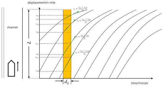
Figure 5.
Schematic calculation of traffic flow characteristics.
represents the cumulative distance covered by all ships in the channel during the time interval , represents the total time traveled by all ships, and denotes the area enclosed by the channel length within the time interval . The formulas for determining the cumulative distance covered by all ships in the channel within the time interval , the cumulative time spent by all vessels, and the area encompassed by the channel length and the time interval are as follows:
where is the time that the ship sails in the channel. is the number of ships in the channel in the time interval. is the length of the channel. and is the average speed of each ship in the channel in the time interval. The formula for calculating the average speed of each ship in the channel in the time interval, , is as follows:
where is the longitudinal displacement of the ship in the channel at the end of the time interval, and is the longitudinal displacement of the ship in the channel at the end of the time interval.
4. Plotting Fundamental Diagram of Waterway Traffic Flow
4.1. Data Processing
Based on pertinent statistics, Shanghai Port achieved the distinction of being the first port worldwide to surpass an annual container throughput of 40 million TEUs in 2017. By 2023, this figure had risen to 4915.8 million TEUs [27]. Furthermore, Shanghai Port has maintained its position as the top-ranked port globally in terms of container throughput for over a decade. The Shanghai harbor boasts abundant water resources, a multitude of navigable vessels, intricate navigation conditions, and a substantial repository of AIS data. Utilizing Shanghai AIS data to assess water traffic conditions and plot the fundamental diagram of waterway traffic flow can offer a theoretical foundation for port and navigation agencies to enhance the organization of waterway traffic, ensuring the safe and efficient management of waterways. Figure 6 displays an illustration depicting specific sections of water within the Shanghai harbor.
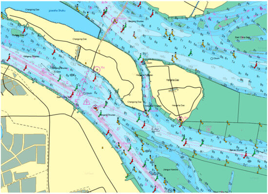
Figure 6.
Specific sections of water within Shanghai Port.
This study focuses on the southern channel in the estuary of the Yangtze River, as depicted in Figure 7 and Table 2. The AIS data from the entire year of 2018 for this waterway are utilized as the primary data source.
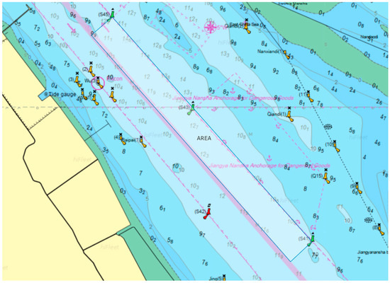
Figure 7.
Diagram of the study waters.
Table 2.
Location of researched waters.
This study required the preprocessing of AIS data in order to implement the plotting process and method of the fundamental diagram of waterway traffic flow suggested in this paper. The preprocessing of AIS data consists of three steps: filtering the AIS data of the waterways, establishing the channel coordinate system, and converting the latitude and longitude coordinates.
- (1)
- Screening of AIS data in the designated study area:
Initially, the latitude and longitude data from each AIS record is extracted. Subsequently, it is determined whether the latitude and longitude coordinates associated with each AIS record fall within the predetermined range specified by the waterway. If the latitude and longitude coordinates of the AIS data fall within the specified range of the waterway, the data are stored in the related waterway’s database. Conversely, if the coordinates are beyond the range, the data are deleted.
By following the aforementioned measures, the quantity of AIS data pertaining to the southern channel was reduced from approximately 880 million to about 2.05 million.
- (2)
- Cleaning the AIS data:
After cleaning and reconstructing AIS data in the designated study area, duplicate entries are removed, and only the relevant AIS data types are saved for the study. These include MMSI, time, longitude, latitude, ship type, ship breadth, ship length, and other pertinent information. These data will serve as a solid foundation for the subsequent stages of the study.
- (3)
- Coordinate system conversion:
The latitude and longitude coordinates of the data coordinates of the channel in this study are (31.23°95′16″ N, 121.79°19′73″ E), and the latitude and longitude coordinates of the ship’s AIS data point in the channel are (, ). The ship’s position information in the Cartesian coordinate system (, ) was obtained by using Formulas (1)–(7) in Section 3 of this paper and the ship’s latitude and longitude coordinates in the AIS data. Table 3 displays a selection of the converted latitude and longitude coordinates.
Table 3.
A selection of the converted latitude and longitude coordinates.
4.2. Subdividing Shipping Lanes
Based on the AIS data of the study waters, the average length and average width of vessels were statistically determined to be 100 m and 18 m, respectively. According to the methodology in Section 3.3, the study waters were divided into the following shipping lanes. Table 4 shows the AIS data statistics for the southern channel in the estuary of the Yangtze River after shipping-lane subdivision.
Table 4.
The statistics for the southern channel in the estuary of the Yangtze River.
Combined with the actual situation of the southern channel in the estuary of the Yangtze River and the subdivision data, when the subdivision width is set at twice the average ship length, the subdivided shipping lane with the most data points of the entry of the ship into the channel is 90~290 m. At this time, the ratio to the total number of vessels accounted for 51.42%, and the ratio to the total number of track points is able to better characterize the traffic flow of the channel.
The AIS trajectory data for ships entering the channel are extracted, with Y values ranging from 90 to 290 m. The spatio-temporal trajectory map of the ship in this subdivided shipping lane is shown by using the time series as the horizontal axis and the displacement of the ship in the X direction as the vertical axis. The resulting trajectory diagram is illustrated in Figure 8, Figure 9 and Figure 10.
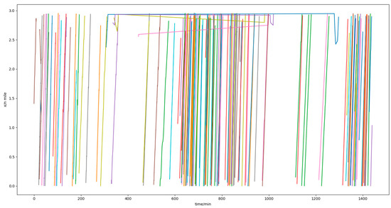
Figure 8.
Sketch of the trajectories of vessels (no shipping-lane subdivision).
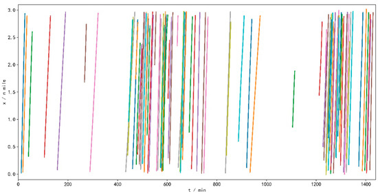
Figure 9.
Sketch of the trajectories of vessels (shipping-lane subdivision: 90–290 m).
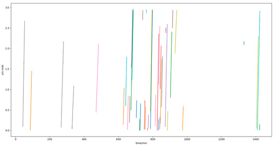
Figure 10.
Sketch of the trajectories of vessels (shipping-lane subdivision: 130–230 m).
By comparing the spatio-temporal trajectory diagrams of ships, it becomes evident that there is a significant amount of data on ship-overtaking behaviors when the shipping lanes are not divided. However, the data on ship-overtaking behaviors decreases noticeably when the shipping lanes are divided. Consequently, the waterway traffic flow characteristics derived from these vessel spatio-temporal trajectory diagrams will differ significantly. Since fundamental diagrams of traffic flow are typically constructed for a single lane, and ship following is closely linked to the fundamental diagram of waterway traffic flow, it is more scientifically and logically sound to plot the fundamental diagram of waterway traffic flow by dividing shipping lanes.
4.3. Fundamental Diagram of Waterway Traffic Flow
Taking min, the characteristic of the traffic flow in the subdivided shipping lane with the value of the ships’ AIS data in the range of m were calculated and plotted, and the fundamental diagram of this shipping lane is shown in Figure 11.
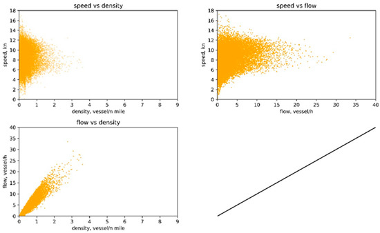
Figure 11.
The fundamental diagram of the researched shipping lane traffic flow.
When analyzing Figure 12, depicting the link between traffic flow and density, researchers discovered that plotting the density separated by certain intervals and taking the maximum value of the traffic flow volume within the intervals will result in the phenomenon of traffic flow hysteresis [28]. In road traffic, the first half of the traffic flow where there is a point of traffic flow hysteresis is the free-flow portion of the traffic flow, and the second half of the traffic flow is the blocked-flow portion of the traffic flow. Hence, Figure 13 likewise substantiates the presence of analogous characteristics in waterway traffic flow, akin to the fundamental pattern of road traffic flow.
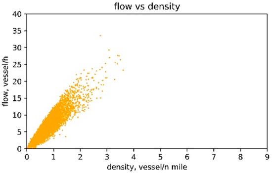
Figure 12.
The fundamental diagram of the researched shipping lane traffic flow.
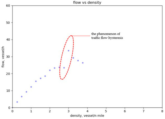
Figure 13.
The fundamental diagram of the researched shipping lane traffic flow (density separated by certain intervals).
Based on the flow–density plot, the densities were subdivided into intervals of , and the highest flow in each density interval was selected to reflect the flow conditions at that interval. A scatter plot displayed the plotted points, and the slope of the tangent line to the curve representing the relationship between flow and density, starting from the origin, represented the free-flow velocity . This slope was extended by following the trend of the scatter plot’s tails until it intersected the horizontal axis, indicating the blockage density at the point of intersection.
The least squares method was employed to fit the scattering points in both the free-flow and blockage sections of the scattering diagram. The least squares fitting relationship for the scattering points in the free-flow section can be expressed as follows: . Similarly, the scattering points in the blockage section can be fitted using the following relationship: . The obtained values for the free-flow velocity , about knots, and the blockage density , approximately 6.5 vessels per nautical mile, are presented in Figure 14.
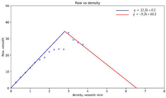
Figure 14.
The fundamental diagram of the researched shipping lane traffic flow with fitted curves (density separated by certain intervals).
5. Conclusions
In this study, AIS data from the research area was primarily analyzed by data cleaning, screening, and data interpolation. The spatio-temporal trajectories of vessels were obtained from the AIS data, which were utilized to compute the characteristics of waterway traffic flow. Moreover, this study proposes a technique for dividing shipping lanes to emphasize the differences between the flow of waterway traffic and road traffic in terms of lane demarcations. By comparing the vessels’ spatio-temporal trajectory diagrams, it was discovered that the proposed method of dividing shipping lanes in this paper can successfully eliminate data that are not relevant to ship following. This allows for a more accurate representation of the real situation of waterway traffic flow in the fundamental diagram of waterway traffic flow. Ultimately, this research employs the acquired traffic flow characteristic data to generate scatter plots, then examines and assesses the correlation among these data points.
The primary contributions of this study mostly lie in the following aspects:
(1) This study reveals the presence of hysteresis in the scatter plot of waterway traffic flow by analyzing the link between flow and density. Additionally, this study identifies blockage density as a critical characteristic of waterway traffic flow. It addresses the issue of calculating the density of blockages in waterway traffic flow by using the fundamental diagram.
(2) This work presents a procedure for plotting fundamental diagrams of waterway traffic flow using AIS data. This enables the extraction of crucial characteristics of waterway traffic flow from vast quantities of AIS data.
Furthermore, the capacity of the waterway depicted in the fundamental diagram can serve as a reference for the departments responsible for waterway management and investment decisions when considering reconstructing or widening the waterway. Similarly, density in the fundamental diagram can provide a basis for waterway traffic authorities to implement traffic management measures.
In the future, when studying the fundamental diagram of canal traffic flow, the following perspectives for future research are proposed:
(1) The data utilized in this study are the 2018 AIS data from the southern channel in the estuary of the Yangtze River. In order to validate the proposed method of constructing a fundamental diagram of maritime traffic flow using AIS data, additional research should be conducted using AIS data from various bodies of water to confirm the feasibility of this method and the universality of the resulting fundamental diagram of traffic flow in the future.
(2) This study focused on analyzing the scatter plot of the fundamental diagram of traffic flow from a macro perspective. This study determined the blockage density of the researched shipping lane based on the scatter plot. However, this study did not examine the blockage density of the researched shipping lane using the equilibrium model of the fundamental diagram of traffic flow. In the future, these two elements should be combined to carry out a study and provide more precise critical metrics of the channel.
(3) Better results can be achieved by using the above methods of subdividing shipping lanes in cases where the question of how to divide shipping lanes is outstanding. Methods of subdividing shipping lanes can be looked into in depth in the future.
Author Contributions
The authors confirm that the contributions to this paper are as follows: conceptualization, S.Z. and Y.L.; data curation, S.Z. and Z.X.; formal analysis, Y.L.; methodology, S.Z. and Y.L.; software, S.Z.; writing—original draft, S.Z.; writing—review and editing, Y.L. and Z.X. All authors have read and agreed to the published version of the manuscript.
Funding
This work was funded by Research and Application Demonstration Project of Key Technologies for Safeguarding of Container vessels in Ningbo Zhoushan Port Based on Intelligent Navigation under grant ZJHG-FW-2024-27, the Shanghai Commission of Science and Technology Project under grants 21DZ1201004 and 2300501900, the Anhui Provincial Department of Transportation Project under grant 2021-KJQD-011, the National Natural Science Foundation of China under grant 51509151, and in part by the Shandong Province Key Research and Development Project under grant 2019JZZY020713.
Institutional Review Board Statement
Not applicable.
Informed Consent Statement
Not applicable.
Data Availability Statement
No new data were created or analyzed in this study. Data sharing is not applicable to this article.
Conflicts of Interest
The authors declare no conflicts of interest.
Notation
Description of variables.
| Flow of waterway | |
| Speed of waterway flow | |
| Density of waterway flow | |
| The length of the channel | |
| The number of ships | |
| The average speed of the ith ship | |
| x | The longitudinal displacement of the ship |
| Average ship’s length | |
| Shipping lane_i | The ith shipping lane |
| B | Average ship’s breadth |
| S | Voyage |
| Latitude difference | |
| Longitude difference | |
| Meridional curvature | |
| Meridional curvature | |
| Difference of meridional curvature | |
| Course | |
| Angle between the datum coordinate and the straight line connecting the AIS data point and the direction of the channel | |
| value corresponding to the AIS data point in the coordinate system of the channel | |
| value corresponding to the AIS data point in the coordinate system of the channel |
References
- Wu, Z. Maritime Traffic Engineering; Dalian Maritime University Press: Dalian, China, 1993. [Google Scholar]
- Huang, Y.; Yip, T.L.; Wen, Y. Comparative analysis of marine traffic flow in classical models. Ocean Eng. 2019, 187, 106195. [Google Scholar] [CrossRef]
- Tasseda, E.-H.; Shoji, R. Macroscopic Traffic Analysis of Vessel Traffic Streams in Tokyo Bay. Annu. Navig. 2015, 191, 16–17. [Google Scholar]
- Qi, L.; Zheng, Z.; Gang, L. A cellular automaton model for ship traffic flow in waterways. Phys. A 2017, 471, 705–717. [Google Scholar] [CrossRef]
- Liu, Y.; Cheng, Y.; Tu, B.; Ni, D. Level of Service Based on Fundamental Diagram of Waterway Traffic Flow. Transp. Res. Rec. J. Transp. Res. Board 2022, 2676, 63–72. [Google Scholar] [CrossRef]
- Feng, H.; Bao, X.; Zhou, J.; Li, S.; Fang, Q. Cellular automata model on AIS-based for variable two-way waterway. J. Ind. Eng. Manag. Data Ser. Parks Wildl. Dep. 2015, 8, 674–692. [Google Scholar]
- Zhang, L.; Yuan, Z.; Yang, L.; Liu, Z. Recent developments in traffic flow modeling using macroscopic fundamental diagram. Transp. Rev. 2020, 40, 529–550. [Google Scholar] [CrossRef]
- Edie, L.C. Discussion of Traffic Stream Measurements and Definitions; Port of New York Authority: New York, NY, USA, 1963.
- Ni, D. Determining Traffic-Flow Characteristics by Definition for Application in ITS. IEEE Trans. Intell. Transp. Syst. 2007, 8, 181–187. [Google Scholar] [CrossRef]
- Treiber, M.; Hennecke, A.; Helbing, D. Congested traffic states in empirical observations and microscopic simulations. Phys. Rev. E 2000, 62, 1805. [Google Scholar] [CrossRef] [PubMed]
- Liu, Y.; Zhuang, S.; Guo, R.; Xiyue, L.; Li, J. Research on the level of service of water transportation based on the perspective of traffic differences. In Proceedings of the 7th International Conference on Transportation Information Safety and Health, Xi’an, China, 4–6 August 2023; pp. 1221–1229. [Google Scholar]
- Greenshields, B.D.; Bibbins, J.R.; Channing, W.S.; Miller, H.H. A study of traffic capacity. Highw. Res. Board Proc. 1935, 14, 448–477. [Google Scholar]
- Yang, L.; Yin, S.; Han, K.; Haddad, J.; Hu, M. Fundamental diagrams of airport surface traffic: Models and applications. Transp. Res. Part B 2017, 106, 29–51. [Google Scholar] [CrossRef]
- Rivera, A.D.d.; Dick, C.T. Illustrating the implications of moving blocks on railway traffic flow behavior with fundamental diagrams. Transp. Res. Part C 2021, 123, 102982. [Google Scholar] [CrossRef]
- Hughes, R.L. A continuum theory for the flow of pedestrians. Transp. Res. Part B 2002, 36, 507–535. [Google Scholar] [CrossRef]
- Botma, H. Method to determine level of service for bicycle paths and pedestrian-bicycle paths. Transp. Res. Rec. 1995, 1502, 38–44. [Google Scholar]
- Pipes, L.A. Car following models and the fundamental diagram of road traffic. Transp. Res. 1967, 1, 21–29. [Google Scholar] [CrossRef]
- Greenberg, I. The log normal distribution of headways. Aust. Road Res. 1966, 2, 14–18. [Google Scholar]
- Cassidy, M.J. Bivariate relations in nearly stationary highway traffic. Transp. Res. Part B 1998, 32, 49–59. [Google Scholar] [CrossRef]
- Ni, D.; Leonard, J.D.; Jia, C.; Wang, J. Vehicle Longitudinal Control and Traffic Stream Modeling. In Proceedings of the Transportation Research Board Meeting, Washington, DC, USA, 22–26 January 2012; pp. 1016–1031. [Google Scholar]
- Aerde, M.V.; Rakha, H. Multivariate Calibration of Single-Regime Speed-Flow-Density Relationships. In Proceedings of the 6th 1995 Vehicle Navigation and Information Systems Conference, Seattle, WA, USA, 30 July–2 August 1995. [Google Scholar]
- Ni, D. Field Theory for Some Traffic Phenomena and Fundamental Diagram. Transp. Res. Rec. 2021, 2675, 1195–1208. [Google Scholar] [CrossRef]
- Shi, X.; Li, X.J.T.R.P.B.M. Constructing a fundamental diagram for traffic flow with automated vehicles: Methodology and demonstration. Transp. Res. Part B Methodol. 2021, 150, 279–292. [Google Scholar] [CrossRef]
- Kang, L.; Meng, Q.; Liu, Q. Fundamental diagram of ship traffic in the Singapore Strait. Ocean Eng. 2018, 147, 340–354. [Google Scholar] [CrossRef]
- Fujii, Y.; Navigation, K.T. Traffic capacity. J. Navig. 1971, 24, 543–552. [Google Scholar] [CrossRef]
- Szlapczynski, R.; Szlapczynska, J. Review of ship safety domains: Models and applications. Ocean Eng. 2017, 145C, 277–289. [Google Scholar] [CrossRef]
- Portshanghai. Key Figures: Container and Cargo Throughputs. Available online: https://www.portshanghai.com.cn/tjsj/index.jhtml (accessed on 13 May 2024).
- Saberi, M.; Mahmassani, H.S. Hysteresis and Capacity Drop Phenomena in Freeway Networks: Empirical Characterization and Interpretation. Transp. Res. Rec. 2013, 2391, 44–55. [Google Scholar] [CrossRef]
Disclaimer/Publisher’s Note: The statements, opinions and data contained in all publications are solely those of the individual author(s) and contributor(s) and not of MDPI and/or the editor(s). MDPI and/or the editor(s) disclaim responsibility for any injury to people or property resulting from any ideas, methods, instructions or products referred to in the content. |
© 2024 by the authors. Licensee MDPI, Basel, Switzerland. This article is an open access article distributed under the terms and conditions of the Creative Commons Attribution (CC BY) license (https://creativecommons.org/licenses/by/4.0/).