Fluid–Structure Interaction Analysis of Manta-Bots with Self-Induced Vertical Undulations during Fin-Based Locomotion

Abstract

Driven by the demands of ocean exploration, an increasing number of manta ray-inspired robots have been designed and manufactured, primarily utilizing flexible skeletons combined with motor-driven mechanisms. However, the mechanical analysis of these designs remains underdeveloped, often relying on simplistic imitation of biological prototypes and typically neglecting the vertical motion induced by pectoral fin flapping. This paper presents a fluid–structure interaction analysis framework that couples rigid body motion with elastic deformation using flexible multibody dynamics and the vortex particle method. An implicit iterative algorithm with Aitken relaxation is employed to address added-mass instability, and the framework has been validated against experimental data. An analysis of a representative manta-bot model shows that self-induced vertical undulations reduce the thrust coefficient by approximately 40% compared to fixed vertical degrees of freedom, while slightly improving overall propulsive efficiency. The study also highlights the critical role of mass distribution in manta-bots, noting that excessive focus on complex pectoral fin movements and large fin mass can significantly reduce thrust by increasing vertical displacement, ultimately proving counterproductive.

1. Introduction

Recent years have witnessed a significant surge in the interest in Automatic Underwater Vehicles (AUVs), which hold a crucial role in underwater exploration [1]. Although the prevailing designs of these vehicles predominantly emulate a submarine configuration, relying on propulsion systems such as hydraulic motors, impellers, waterjets, or propellers, their operational characteristics are hindered by several drawbacks. These conventional means of propulsion, while undoubtedly powerful and robust, generate considerable noise, necessitate intricate mechanical architectures, involve substantial weight, and are characterized by conspicuously detectable attributes [2].

Simultaneously, the utility of fish-inspired bionic robots, previously explored as an alternative approach, has encountered limitations. Despite their biomimetic nature, these robots exhibit pronounced deformation during motion, rendering them challenging to control effectively and unsuitable for stealthy surveillance missions [3].

Against this backdrop, the manta ray-inspired flapping mechanism has emerged as a promising avenue of investigation. This novel propulsion paradigm combines the agility and maneuverability akin to its more conventional counterparts, yet significantly reduces the disturbances typically associated with them. As a result, it has garnered increasing interest within the scientific community, as researchers seek to harness its potential for quieter, more streamlined, and covert underwater operations [4].

1.1. Fin Structures of Manta-like AUVs

The design of the pectoral fin skeleton structure and actuation mechanism is central to the development of bioinspired manta ray AUVs. Early research, inspired by biological prototypes, introduced sophisticated transmission systems and rigid multi-segmented skeletons to mimic the motion of real manta rays. However, these designs proved cumbersome and intricate, with fully rigid pectoral fins necessitating an actuator for each degree of freedom [5]. This resulted in exceptionally complex drive and transmission systems that were spatially constrained and challenging to implement. Additionally, these designs overlooked the flexible deformation of pectoral fins, despite growing evidence that such flexibility can enhance propulsive efficiency [6,7].

Table 1. Characteristics of motor-driven bioinspired manta ray robots developed in recent years.

Authors	Illustration	Features
He et al. [6] Cao et al. [8] Zhou et al. [9]		Multi-beams with separated servos Chordwise flexibility generated by phase difference of servos Stiff or elastic beams with soft skin
Lu et al. [10] Chew et al. [11]		One servo with one degree of freedom (DOF) Beam responds to spanwise flexibility Ribs respond to chordwise flexibility Open frame of elastic structure with soft skin
Chen et al. [12] Liu et al. [13] Xing et al. [14]		Pitch and roll DOFs controlled by servos Closed frame of elastic structure with soft skin; or integrated elastic fin

presents representative bioinspired manta ray robots developed in recent years. These robots commonly employ one or more relatively stiff fin rays, augmented by structural beams and joints, with servo motors located at the base or joints serving as actuators. This type of design leverages structural flexibility while allowing for a degree of control, representing the mainstream approach currently feasible for production. Some designs, however, use compressed air or novel flexible actuators to drive pectoral fins made entirely of flexible materials. These approaches remain highly immature, struggling with the control of three-dimensional deformation.

1.2. Numerical Simulations

Numerical simulation plays a significant role in the design of biomimetic underwater robots, as well as in understanding their biomechanical principles. The complexity of accurate modeling arises from the intricate interaction of various physical fields involved in the flapping motion of the pectoral fins. This paper outlines different approaches to simulation, categorized by their complexity and scope, illustrated in Figure 1.

Approach A focuses on fluid simulations with prescribed motion boundary conditions. This approach is widely used in biological studies, where detailed morphologies of swimming manta rays are obtained through high-speed cameras or Particle Image Velocimetry (PIV) and then input into Computational Fluid Dynamics (CFD) solvers. The key challenges involve obtaining accurate morphological data and meticulously setting motion boundary conditions, often utilizing techniques such as moving meshes, overlapping meshes, or immersed boundary methods to accommodate the dynamic nature of the biological models [15].

Approach B involves simulations that couple fluid dynamics with rigid body mechanics, accounting for the motion of rigid bodies [16]. This approach is common in the early design stages of underwater gliders or biomimetic mantabots. For example, Huang et al. [17] analyzed the hydrodynamics of a bioinspired robot, exploring the relationship between fin flapping frequency and robot speed, and examining stability during different maneuvers and forward swimming.

Approach C incorporates elastic deformations into the simulation, reflecting the actual forces exerted by fluids on structures. This level of complexity is typically seen in studies of individual flexible wings rather than complete robotic systems. Techniques range from employing pseudo-rigid body dynamics (PRBD) to introduce elasticity via flexible connections among rigid segments [18] to directly integrating derived elastic deformation formulas into the fluid equations’ source terms [19].

Approach D represents a comprehensive simulation framework that integrates rigid body motions, elastic deformations, and fluid dynamics. Utilizing flexible multibody dynamics for structural modeling, this approach captures the interactions between rigid and elastic deformations in wing structures and addresses the overall displacement and deformations induced by fluid forces on the robot.

Each approach has its strengths and challenges. Pure fluid simulations (Approach A) excel in isolating and studying fluid phenomena with high precision, ideal for fundamental research into biomechanical mechanisms. However, as one moves towards more integrated simulations involving multiple physical fields (Approach B through Approach D), the complexity increases significantly. These multifaceted simulations require a careful balance between accuracy and computational efficiency, as the inclusion of additional physical phenomena enriches the model’s realism but also increases the computational burden. The choice of approach depends on the specific objectives of the study, ranging from detailed investigations of fluid dynamics to comprehensive evaluations of the robot’s overall performance under various conditions.

1.3. Research Objectives

In real-world organisms that rely on flapping propulsion, it is quite evident that their bodies exhibit an up-and-down motion corresponding to the flapping of their wings or pectoral fins. This motion results from the reactive forces generated by the fluid medium against the flapping motion, as well as the inertial effects arising from changes in mass distribution and the center of gravity. Taking the Common Murre (Uria aalge) as an example, we compare its flight trajectories in air and underwater, as shown in Figure 2a. The figure is divided into two parts: the upper part shows video stills of the murre flying in the air, while the lower part displays video stills of the murre swimming underwater [20]. Due to the limitations of video representation, we manually traced the murre’s movement trajectories. It is evident that for the same species, the undulating motion caused by flapping is more pronounced and has a larger amplitude when moving underwater. This can be understood from the perspective of medium density, as water is approximately 833 times denser than air, resulting in significantly greater forces. These observations indicate that organisms or underwater vehicles relying on pectoral fin flapping propulsion will experience body undulations due to the flapping motion (see Figure 2b). However, due to the limitations of traditional perspectives and modeling theories, this effect has often been neglected in simulation analyses.

In this study, we develop a fast, general, and strongly coupled 3D fluid–structure Interaction (FSI) simulation framework that integrates the Vortex Particle Method (VPM) with Flexible Multibody Dynamics (FMBD). This framework is capable of directly accounting for the nonlinear dynamics between vertical motion and pectoral fin deformation. The coupled algorithm facilitates the exchange of motion (from the FMBD solver to the VPM solver) and loads (from the VPM solver to the FMBD solver) at the fluid–structure interface in an implicit manner. Specifically, at each time step, iterations are performed until the convergence criterion is met. The mapping method for the incompatible structural and aerodynamic domains is based on the conservation of work exchanged between them. This mapping is achieved through a 3D interpolation of the mesh/grids at the interface between the two domains using radial basis functions (RBFs).

The structure of this paper is organized as follows. Section 2 introduces the proposed fluid–structure interaction framework and its validation. In Section 3, we describe a representative model of a bio-inspired manta ray robot and the criteria for selecting its parameters. Section 4 applies the proposed FSI analysis framework to a scenario with a fixed vertical degree of freedom, followed by a detailed analysis. Section 5 extends this analysis by allowing the vertical degree of freedom to vary due to self-induced undulations from fin movements, and the results are compared with those obtained in Section 4. Finally, the conclusions are presented in Section 6.

2. Method and Validation

2.1. Flexible Multibody Dynamics

The system configuration of n rigid bodies in 3D space is defined using generalized coordinates $\mathbf{q}=[{\mathbf{r}}_1^T,{\mathsf{\epsilon }}_1^T,\dots ,{\mathbf{r}}_n^T,{\mathsf{\epsilon }}_n^T]\in {\mathbb{R}}^{7n}$, where ${\mathbf{r}}_j$ and ${\mathsf{\epsilon }}_j$ represent the center of mass and Euler parameters, respectively. The velocity vector $\mathbf{v}\in {\mathbb{R}}^{6n}$ is related to $\dot{\mathbf{q}}$ via $\dot{\mathbf{q}}=\mathbf{L}\left(\mathbf{q}\right)\mathbf{v}$, with $\mathbf{L}\left(\mathbf{q}\right)$ being a block diagonal matrix involving the transformation matrix $\mathbf{G}$.

The dynamics are formulated as a set of differential-algebraic equations:

$$\dot{\mathbf{q}}=\mathbf{L}\left(\mathbf{q}\right)\mathbf{v}$$

(1)

$$\mathbf{M}\left(\mathbf{q}\right)\dot{\mathbf{v}}=\mathbf{f}(t,\mathbf{q},\mathbf{v})-{\mathbf{g}}_{\mathbf{q}}^T(\mathbf{q},t)\widehat{\mathsf{\lambda }}$$

(2)

$$\mathbf{0}=\mathbf{g}(\mathbf{q},t)$$

(3)

For flexible bodies undergoing large deformations, the Absolute Nodal Coordinate Formulation (ANCF) is used, utilizing nodal positions and gradients. This includes gradient-deficient cable and shell elements which simplify the mass matrix and improve computational efficiency.

For further theoretical details and numerical validations of the models and methods described, refer to the author’s previous work [21] and the open-source software Chrono 8.0.0 [22,23].

2.2. Unsteady Panel and Vortex Particle Hybrid Method

In the context of inviscid, incompressible, and irrotational flow, the velocity field can be obtained by solving Laplace’s equation, subject to appropriate velocity boundary conditions on the body surface and far-field. The continuity equation for incompressible potential flow, governed by Laplace’s equation, is given by:

$${\nabla }^2\varphi =0$$

(4)

where $\varphi$ is the velocity potential, and the velocity of an irrotational flow can be defined as:

$$\mathbf{V}=\nabla \varphi .$$

(5)

To solve Laplace’s equation, we employ Green’s second identity, which yields a general solution in terms of surface integrals. Assuming a thin wake surface, we represent it as a sum of doublet distributions on the wake surface $S_w$ and a sum of source and doublet distributions on the body surface $S_B$. The resulting integral form is as follows:

$$\beta \varphi \left(\mathbf{x}\right)=-{\int \int }_{S_B}[G\nabla \sigma ·\mathbf{n}-\mu \nabla G·\mathbf{n}]dS+{\int \int }_{S_W}\mu \nabla G·\mathbf{n}dS$$

(6)

where G is Green’s function, $\beta$ is the solid angle, n is the outward unit normal vector of the surface, and $\sigma$ and $\mu$ are the strengths of the source and doublet singular elements, respectively [24].

The doublet strength is defined as the difference between the external and internal potential on the solid boundary:

$$\mu ={\varphi }_i-\varphi$$

(7)

while the source strength is given by the discontinuity in the normal derivative of the velocity potential on the solid boundary:

$$\sigma =({\varphi }_i-\varphi )·\mathbf{n}=\frac{\partial {\varphi }_i}{\partial n}-\frac{\partial \varphi }{\partial n}$$

(8)

Substituting the definitions of the source and doublet strengths, the general solution can be rearranged as:

$$\varphi \left(\mathbf{x}\right)=-\frac{1}{4\pi }{\int \int }_{S_B}\left[\sigma \left(\frac{1}{r}\right)-\mu \nabla \left(\frac{1}{r}\right)·\mathbf{n}\right]dS+\frac{1}{4\pi }{\int \int }_{S_W}\mu \nabla \left(\frac{1}{r}\right)·\mathbf{n}dS$$

(9)

To numerically solve the integral equation, the body and wake surfaces are discretized into a number of rectilinear panels, comprising N body surface panels and $N_W$ additional wake panels with constant-strength singularities. The influences of body panel k and wake panel j at point P can be computed using Equation (10), where the total inner potential is set equal to the freestream potential to satisfy the Dirichlet boundary condition at each of the collocation points.

$$\begin{array}{cc}\hfill & \sum _{k=1}^N\frac{1}{4\pi }{\int \int }_{S_B}\mu \nabla \left(\frac{1}{r}\right)·\mathbf{n}dS\hfill \\ \hfill & +\sum _{j=1}^{N_W}\frac{1}{4\pi }{\int \int }_{S_W}{\mu }_W\nabla \left(\frac{1}{r}\right)·\mathbf{n}dS\hfill \\ \hfill & -\sum _{k=1}^N\frac{1}{4\pi }{\int \int }_{S_B}\sigma \left(\frac{1}{r}\right)dS=0\hfill \end{array}$$

(10)

The integral equation for finding the unknown doublet distribution ($\mu$) on the body surface can be established as a linear algebraic equation, as in Equation (11). Here, ${\mu }_W$ is the strength of wake doublets, which can be expressed in terms of the unknown surface doublets (${\mu }_k$) by enforcing the Kutta condition as in Equation (12). The Kutta condition implies that the wake doublets are related to the difference between the doublet strengths of the upper and lower panels of the trailing edge (see Figure 3). Additionally, the source strength ($\sigma$) can be determined by applying the zero normal flow condition on the surface, defined as in Equation (13) with the local kinematic velocity.

$$\begin{array}{cc}\hfill & \sum _{k=1}^N{C}_k{\mu }_k+\sum _{j=1}^{N_W}{C}_j{\mu }_{W,j}-\sum _{k=1}^N{B}_k{\sigma }_k=0,where\hfill \\ \hfill & C_k\equiv {\left.\frac{1}{4\pi }{\int \int }_{S_B}\nabla \left(\frac{1}{r}\right)·\mathbf{n}dS\right|}_k\hfill \\ \hfill & C_j\equiv \frac{1}{4\pi }{\int \int }_{S_W}\nabla \left(\frac{1}{r}\right)·\mathbf{n}dS{|}_j\hfill \\ \hfill & B_k\equiv \frac{1}{4\pi }{\int \int }_{S_B}\left(\frac{1}{r}\right)dS{|}_k\hfill \end{array}$$

(11)

$${\mu }_W={\mu }_u-{\mu }_l$$

(12)

$$\sigma =-({\mathbf{V}}_{\infty }+{\mathbf{V}}_{\mathrm{rel}}+\mathsf{\Omega }\times \mathbf{r})·\mathbf{n}$$

(13)

Note, that the strengths of the source and wake doublet are known at each time step. Moving the source term of Equation (11) to the right-hand side of the equation results in a linear system of N equations with the unknown ${\mu }_k$, in the following form:

$$\sum _{k=1}^N{A}_k{\mu }_k=\sum _{k=1}^N{B}_k{\sigma }_k$$

(14)

$$\left[\begin{array}{cccc}{a}_{11}& a_{12}& \cdots & a_{1N}\\ a_{21}& a_{22}& \cdots & a_{2N}\\ ⋮& ⋮& \ddots & ⋮\\ a_{N1}& a_{N2}& \cdots & a_{NN}\end{array}\right]\left\{\begin{array}{c}{\mu }_1\\ {\mu }_2\\ ⋮\\ {\mu }_N\end{array}\right\}=\left\{\begin{array}{c}{\mathrm{RHS}}_1\\ {\mathrm{RHS}}_2\\ ⋮\\ {\mathrm{RHS}}_N\end{array}\right\}$$

(15)

Once the linear system of equations is solved, the local velocity components of the surface panel coordinates and the pressure coefficients can be evaluated. Furthermore, the aerodynamic loads are then obtained by integrating the pressure over the lifting surface.

Now that we have discussed the solution of the boundary element on the surface of the object, we will proceed to discuss the modeling method of the trailing vortex. Assuming that the flow field is incompressible, the three-dimensional incompressible Navier–Stokes equations can be expressed in the velocity-vorticity form:

$$\frac{\partial \omega }{\partial t}+u·\nabla \omega =\nabla u·\omega +\nu {\nabla }^2\omega$$

(16)

where $\nu$ denotes the kinematic viscosity coefficient, $\omega$ represents the vorticity, and u is the velocity. The first term on the right-hand side of Equation (16) corresponds to the stretching term, while the second term represents the viscous dissipation term. By adopting a Lagrangian description of the vorticity field, we can discretize it into N vortex particles carrying vorticity, volume, and mass. Consequently, the vorticity field can be reconstructed as

$$\omega (x,t)=\sum _{i=1}^N{\alpha }_i{\eta }_{\epsilon }(x-x_i)$$

(17)

where ${\mathbf{x}}_i$ denotes the position of particle i; ${\mathsf{\alpha }}_i$ represents the vorticity vector of particle i and ${\eta }_{\epsilon }\left(\rho \right)$ is the Gaussian smoothing function

$${\eta }_{\epsilon }\left(\rho \right)=\frac{1}{{\left(2\pi \right)}^{3/2}{\epsilon }^3}{\mathrm{e}}^{-{\rho }^2/2}$$

(18)

where $\epsilon$ is the smoothing parameter and $\rho =\left|\mathbf{x}-{\mathbf{x}}_i\right|/\epsilon$ is the nondimensional distance.

Based on the reconstructed vorticity field, the Navier–Stokes equations can be split into

$$\frac{d\mathbf{x}}{dt}=\mathbf{u}(\mathbf{x},t)$$

(19)

$$\frac{d\mathsf{\alpha }}{dt}=\nu {\nabla }^2\mathsf{\alpha }+\mathbf{\nabla }\mathbf{u}·\mathsf{\alpha }$$

(20)

where Equation (19) describes the transport effect of the vorticity and Equation (20) represents the dissipation and stretching effects of the vorticity. To model the transport effect of the vorticity, we employ the Biot–Savart law to obtain the velocity of the particle points and then utilize numerical integration to determine the position of the vortex particles $x\left(t\right)$. Meanwhile, we can employ the particle strength exchange method and direct solution method to model the dissipation and stretching effects of the vorticity, respectively, but we will not elaborate on these methods here due to space limitations.

Finally, we will explore the conversion between the dipole panel and the vortex particle. According to the Hess equivalence principle [25], the induced velocity of a dipole panel with strength $\mu$ at any point in space is identical to that of a boundary vortex with strength $\mu$, i.e.,

$$u_{\mu }\left(x\right)=-\frac{1}{4\pi }{\int }_S\gamma ·\frac{\mathbf{r}}{r^3}dS+\frac{1}{4\pi }{\int }_{C_w}\mu ·\frac{d\mathbf{l}\times \mathbf{r}}{r^3}$$

(21)

where $\mathbf{l}$ denotes the line vortex vector and $C_w$ represents the boundary line of the trailing vortex panel [26]. By integrating the equivalent surface vorticity strength $\gamma$ and line vorticity strength $\mu$ of the trailing vortex panels, we can obtain the vorticity strength of the vortex particle at the center of the panel. At each time step, we only need to replace the second group of trailing vortex panels with vortex particles (see Figure 3), and then solve the Navier–Stokes equations to determine the spatial distribution of the trailing vortex.

The open-source software, DUST 0.8.2-b, utilized in this study employs a hybrid approach, combining the fundamental theories outlined in this article with the Cartesian Fast Multipole Method (FMM). This synergy enables a significant reduction in computational complexity, from $\mathcal{O}\left(N^2\right)$ to $\mathcal{O}(NlogN)$. For further details on the testing and validation of this methodology, the reader is referred to the original literature [27].

2.3. Partitioned FSI Coupling Techniques

2.3.1. Mapping Techniques

The exchange of data between the fluid and structural domains can be categorized into two primary types: (i) the displacement of structural nodes translating into fluid motion, and (ii) force vectors at control points on the fluid mesh impacting structural nodes. The former can be mathematically represented as

$$\mathbf{h}=\mathsf{\Phi }\mathbf{x}$$

(22)

where $\mathbf{h}$ represents the displacement vector of the fluid mesh grid, $\mathbf{x}$ denotes the displacement vector of the structural nodes, and $\mathsf{\Phi }$ is the interpolation matrix.

Based on the principles of virtual work, the force ${\mathbf{F}}_h$ on the fluid mesh and its corresponding force ${\mathbf{F}}_a$ on the structural nodes must perform the same amount of virtual work. This relationship is expressed as

$$\delta {\mathbf{h}}^T{\mathbf{F}}_h=\delta {\mathbf{x}}^T{\mathbf{F}}_a$$

(23)

where $\delta h^T$ and $\delta x^T$ are the virtual displacements of the fluid mesh and structural nodes, respectively. By combining Equations (22) and (23), we derive

$$\delta {\mathbf{x}}^T({\mathbf{F}}_a-{\mathsf{\Phi }}^T{\mathbf{F}}_h)=0.$$

(24)

Given that $\delta \mathbf{x}$ can be arbitrary, Equation (24) becomes equivalent to

$${\mathbf{F}}_a={\mathsf{\Phi }}^T{\mathbf{F}}_h$$

(25)

which establishes the method for transferring forces from the fluid domain to the structural domain. With Equation (22) defining the transfer of displacements from the structural domain to the fluid domain, the data exchange process is comprehensively described.

The construction of the interpolation matrix $\mathsf{\Phi }$ is critical to the data-transfer procedure. Previous research has developed two main types of methods: (i) local interpolation methods such as mapping interpolation [28], weighted residuals, and constant-volume conversion, and (ii) global interpolation methods including spline functions and the Shepard method. Local interpolation methods are direct and fast but require specific algorithms to locate mapping points on complex geometries, whereas global interpolation methods are more accurate but slower, as they assume that quantities at any point in the domain can be derived from information at other points in the physical field (solid or fluid). In this study, we employ Compactly Supported Radial Basis Functions (CS-RBFs), which balance the accuracy and efficiency of both local and global interpolation methods.

CS-RBFs incorporate compact support, which means that only the effects within a specified support area are considered, ignoring those outside this area. This approach transforms the full matrix in ordinary RBF interpolation into a sparse matrix. For theoretical details on this method, refer to [29,30]. The function utilized here is defined as

$$\varphi \left(R\right)={(1-R)}_{+}^6\left(35R^2+18R+3\right)$$

(26)

where $a_{+}=max\{a,0\}$ and $R=\left|\right|x-x_i\left|\right|/r_i$, with $r_i$ being the radius of the compact support.

2.3.2. Coupling Algorithms

In FSI simulations, the Dirichlet-Neumann partitioning approach is commonly employed. This approach solves the fluid problem based on the prescribed displacement on the fluid–structure interface and applies a stress boundary condition on the wet boundary of the structural problem. Given a prescribed fluid interface displacement ${\mathbf{d}}_f^{\mathsf{\Gamma }}$, the fluid interface force can be obtained by applying the nonlinear Dirichlet operator $\mathcal{F}$:

$${\mathbf{t}}_f^{\mathsf{\Gamma }}=\mathcal{F}\left({\mathbf{d}}_f^{\mathsf{\Gamma }}\right).$$

(27)

Similarly, a nonlinear Neumann operator $\mathcal{S}$ can be defined to relate the force acting on the solid interface to the solid interface displacement:

$${\mathbf{d}}_s^{\mathsf{\Gamma }}=\mathcal{S}\left({\mathbf{t}}_s^{\mathsf{\Gamma }}\right).$$

(28)

The coupling conditions expressed by Equations (27) and (28) can thus be rewritten as a fixed-point problem:

$${\mathbf{d}}^{\mathsf{\Gamma }}=\mathcal{S}\left(-\mathcal{F}\left({\mathbf{d}}^{\mathsf{\Gamma }}\right)\right).$$

(29)

Here, ${\mathbf{d}}^{\mathsf{\Gamma }}$ represents the common displacement on the fluid and solid interfaces, while $\mathcal{S}$ and $\mathcal{F}$ can be viewed as black-box solvers for the solid and fluid problems, respectively. To facilitate further discussion, we can reformulate the fixed-point equation more explicitly as:

$${\mathbf{d}}^{\mathsf{\Gamma }}=\mathcal{S}\circ \mathcal{F}\left({\mathbf{d}}^{\mathsf{\Gamma }}\right)=\mathcal{T}\left({\mathbf{d}}^{\mathsf{\Gamma }}\right)$$

(30)

where $\mathcal{T}$ represents the overall nonlinear operator.

Solving the fixed-point problem (Equation (30)) can be achieved using two classes of coupling algorithms. The first approach is explicit coupling, where the solution at the previous time step is directly used to compute the solution at the current time step. This is mathematically represented as:

$${\mathbf{d}}^{k+1}=\mathcal{T}\left({\mathbf{d}}^k\right).$$

(31)

In this approach, the results from the previous time step ($t=k$) are directly used to compute the solution at the current time step ($t=k+1$), with the two solvers alternating in their computation.

Alternatively, the fixed-point problem can be solved implicitly using a Block Gauss-Seidel (BGS) iteration, as illustrated in Figure 4. The simplest algorithm in this class is given by:

$${\mathbf{d}}^{k+1}=\mathcal{T}\left({\mathbf{d}}^k\right)={\tilde{\mathbf{d}}}^k,\mathrm{until}\parallel {\mathbf{r}}^k\parallel =\parallel {\tilde{\mathbf{d}}}^k-{\mathbf{d}}^k\parallel <{\epsilon }_{\mathrm{FSI}},$$

(32)

where the residual ${\mathbf{r}}^k=\mathcal{T}\left({\mathbf{d}}^k\right)-{\mathbf{d}}^k={\tilde{\mathbf{d}}}^k-{\mathbf{d}}^k$ is defined in the same way for all implicit coupling schemes. The tolerance ${\epsilon }_{\mathrm{FSI}}$ is a user-defined parameter. However, in some cases, it can be challenging or even impossible to ensure convergence of the BGS iteration, particularly when the solid-to-fluid density ratio is close to or lower than one, a phenomenon known as added-mass effects.

To enhance or ensure convergence, relaxation can be introduced in Equation (32). The modified algorithm is given by:

$$\begin{array}{cc}\hfill {\mathbf{d}}^{k+1}& =\mathcal{T}\left({\mathbf{d}}^k\right)+\left({\omega }^k-1\right)\left(\mathcal{T}\left({\mathbf{d}}^k\right)-{\mathbf{d}}^k\right)\hfill \\ \hfill & ={\tilde{\mathbf{d}}}^k+\left({\omega }^k-1\right)\left({\tilde{\mathbf{d}}}^k-{\mathbf{d}}^k\right),\mathrm{until}\parallel {\mathbf{r}}^k\parallel =\parallel {\tilde{\mathbf{d}}}^k-{\mathbf{d}}^k\parallel <{\epsilon }_{\mathrm{FSI}}.\hfill \end{array}$$

(33)

The relaxation parameter $\omega$ can be constant (static relaxation) or vary from one iteration to another (dynamic relaxation). In the case of dynamic relaxation, a common strategy for updating $\omega$ is Aitken relaxation:

$${\omega }^k=-{\omega }^{k-1}\frac{{\mathbf{r}}^{k^{\mathrm{T}}}\left({\mathbf{r}}^k-{\mathbf{r}}^{k-1}\right)}{{\left|\left|{\mathbf{r}}^k-{\mathbf{r}}^{k-1}\right|\right|}^2}$$

(34)

The parameter $\omega$ takes values between 0 (no evolution of the displacements) and 1 (no relaxation). Typically, an upper limit ${\omega }_{max}<1$ is imposed by the user to prevent divergence. The BGS coupling with Aitken relaxation has been successful in solving strongly coupled problems in most cases. The capabilities of this coupling scheme, implemented in the open-sourced library preCICE [31], are utilized in this work.

2.4. Validation

To validate the efficacy of our proposed method, we utilized a well-documented experimental setup by Heathcote et al. [32], which involved a flexible rectangular wing subjected to harmonic heave motion within a water tunnel. This setup has been widely employed by various researchers [33,34,35] to benchmark their numerical analyses. Focusing on a NACA0012 profile with dimensions of chord $c=0.1\mathrm{m}$ and semi-span $s=0.3\mathrm{m}$, our validation adopts the most compliant wing configuration from Heathcote’s study, characterized by its polydimethylsiloxane composition stiffened with a thin aluminum layer. The estimated fundamental structural frequency of this model was approximately 1.5 Hz. The structural stiffness was primarily attributed to the aluminum sheet, which we modeled using a rectangular plate composed of ANCF shell elements; see

Table 2. Properties of the simulation plate model.

Parameter	Value	Units
Chord	0.1	m
Span	0.3	m
Young’s modulus	70	GPa
Density	${10}^5$	kg/m3
Fundamental frequency	1.517	Hz

for detailed specifications.

The wing root was subjected to a prescribed displacement, $s=a_{\mathrm{root}}cos\omega t$, as depicted in Figure 5b. The simulation parameters, including the Reynolds number, reduced frequency, and Strouhal number, were adjusted to match the experimental conditions. Figure 5a illustrates the deformation of the wing and the vortex particles in the wake at a specific time step during the VPM simulation.

A key aspect of our reassessment involves a judicious comparison between our VPM program and the well-established FLUENT 2021R1 software. By adopting FLUENT’s overset grid and dynamic mesh capabilities alongside the SST $k-\omega$ turbulence model, we aim for a rigorous benchmarking process. Notably, despite FLUENT’s utilization of an 8-core parallel setup on an Intel i7-11700 platform with a large cell count of 1,134,823, the simulation duration was significantly longer at 3646 min, compared to the VPM’s notably expedient 7-min run time.

Our reassessment includes a meticulous investigation of the displacement profiles at the wing’s leading edge (Figure 6a). By normalizing the root displacement, we facilitate a more nuanced comparison that elucidates subtle variations in amplitude and phase across the span.

The graphical comparison in Figure 6b illustrates the concurrence among experimental outcomes, FLUENT’s predictions, and the VPM’s output. Although minor disparities exist—experiment: amplitude 1.76, phase lag $-{117}^{\circ }$; FLUENT: amplitude 1.69, phase lag $-{114}^{\circ }$; VPM: amplitude 1.84, phase lag $-{113}^{\circ }$—these are within acceptable margins, thereby lending credence to the reliability and accuracy of the proposed FSI methodology.

In conclusion, this prudent reassessment not only affirms the validity of our method but also thoughtfully explores its computational efficacy and compatibility with recognized simulation frameworks, offering a nuanced perspective on a classical benchmark in fluid–structure interaction research.

3. Model Description

In this section, we present the methodology for describing the geometric outline of a manta ray-inspired robot and elucidate the process of constructing its structural skeleton. We conclude by outlining the rationale behind the selection of its basic dimensions and motion parameters.

The hydrodynamic grid geometry (i.e., flow field mesh) of the biomimetic manta robot, as depicted in Figure 7, is characterized by the distinct shape features and functional aspects of a manta ray. The robot is conventionally regarded as comprising two principal components: the body and the pectoral fins. It is judiciously partitioned into three segments, as shown in Figure 7. Ref. [36] revealed that the maximum thickness of a typical manta ray’s body is approximately 2/9 of its longitudinal length. This attribute endows it with thickness distribution characteristics akin to those of the NACA0022 airfoil. Consequently, the NACA0022 profile is chosen as the basis for Slice 1 in our design. To facilitate a smooth transition from the body to the pectoral fins, Slice 2 adopts the NACA0016 airfoil as its foundation, while Slice 3 employs the NACA0008 airfoil. Intermediary sections between these three fundamental profiles are obtained through linear interpolation of the contour lines of their respective adjacent base profiles.

With reference to extant biomimetic robot configurations and biological anatomical outlines, informed by previous research, the outline description functions for the proposed robot’s silhouette are given by Equations (35) and (36). Note that within these equations, x and y represent normalized values, specifically $x=x_{real}/L_{chord}$ and $y=y_{real}/L_{span}$.

For the leading edge profile, we have the fitting function:

$$x_{LE}\left(y\right)=\left\{\begin{array}{cc}3.62023y^2+0.23784y,\hfill & \mathrm{for}0\le y<0.176\hfill \\ 0.332543y^2+0.329804y+0.085654,\hfill & \mathrm{for}0.176\le y\le 1.0\hfill \end{array}\right.$$

(35)

For the trailing edge profile, the fitting function is as follows:

$$\begin{array}{c}\hfill x_{TE}\left(y\right)=\left\{\begin{array}{cc}-1.451844y^2+0.050979y+1.0,\hfill & \mathrm{for}0\le y<0.176\hfill \\ 0.696544y^2-1.036369y+1.124825,\hfill & \mathrm{for}0.176\le y\le 1.0\hfill \end{array}\right.\end{array}$$

(36)

To investigate the impact of grid density on the accuracy of VPM solutions, we varied the number of grid divisions in the chordwise direction ($N_x$) and the spanwise direction ($N_y$). Under a freestream velocity of $\mathbf{V}={(1.0,0.0,0.2)}^T$, we computed the total force on a static manta ray mesh, with the results presented in

Table 3. Grid Independence Verification.

Mesh Level	${\mathit{N}}_{\mathit{x}}$	${\mathit{N}}_{\mathit{y}}$	Total Meshes	$\left|\mathbf{F}\right|$
Ultra Fine	20	60	2400	819.22
Fine	15	40	1200	821.93
Medium	10	30	600	823.64
Coarse	5	20	200	661.83

. It can be observed that once the grid reaches a certain density, the solution accuracy remains nearly unchanged. Considering both computational efficiency and shape fidelity, we selected a grid with $N_x=15$ and $N_y=40$ (Fine Mesh) for subsequent calculations.

In delving deeper into the structural realization of the biomimetic manta robot, we find that the prevailing design approach centers around a skin-on-frame model. The core concept of this design is to integrate rigid and flexible materials to emulate the distinctive motion characteristics of manta ray pectoral fins in nature.

Section 1.1 reveals that the power transmission mechanism in such robots primarily relies on a flexible skeleton, which serves as both the primary conduit for force and torque transmission and, to some extent, defines the overall morphology of the robot. This skeletal structure typically comprises a series of main beams distributed spanwise, functioning as the primary load-bearing structures of the pectoral fins. Along the chordwise direction, there is a set of rib beams that interconnect with the main beams at various spanwise locations to collectively provide effective support to the flexible fins, as depicted in Figure 8.

Table 4. Parameters of Main and Rib Beams in the Manta-bot Skeleton.

Beam ID	Node Pair	w (cm)	h (cm)	E (GPa)	M (kg)
1	1–7	5	8.5	150	6.442
2	7–12	3	3	70	1.137
3	12–18	1	1	50	0.152
4	2–27	3	3	100	2.187
5	7–32	1	1	50	0.135
6	12–34	1	1	50	0.054

provides detailed information about each beam, which can be interpreted as follows: Beam ID represents a unique identifier for each beam; Node Pair denotes the node numbers at the starting and ending points of each beam, respectively; w and h refer to the width and height of the rectangular cross-section of each beam; Elastic Modulus (E) indicates the elastic properties of each beam and Mass (M) corresponds to the weight or mass of each beam.

Furthermore, a drive motor is installed at the root node to generate flapping motion about the x-axis. This configuration enables the robot to simulate the graceful and efficient swimming style of manta rays using a minimal number of degrees of freedom.

Based on publicly available literature data, we can discern that different swimming speeds are exhibited by manta rays in various contexts. These speeds range from 0.25 to 0.47 m/s during foraging, 0.97 m/s during migration, 2.78 to 4.17 m/s during courtship, 4.43 m/s prior to breaching the water surface, and a turning speed of 1.42 ± 0.50 m/s measured from videos. Considering these data in conjunction with experimental conditions and simulation requirements, we first select a moderate cruising speed as the initial value for our simulation, specifically 1 m/s. This velocity encompasses typical dolphin swimming speeds while not being overly extreme, thereby facilitating stable simulation progression.

Having determined the speed, we next consider the flapping frequency and amplitude of the pectoral fins. Literature provides a range of fin beat frequencies from 0.4 to 1.2 Hz, potentially higher in emergency situations, but for simulation stability, we choose a moderate value of 0.5 Hz. Additionally, the literature indicates that the ratio of fin tip flapping amplitude to fin base length is generally greater than or equal to 0.5, an important parameter reflecting manta ray locomotion.

Lastly, we establish several other simulation parameters, such as span length (3.2 m), chord length (1.6 m), and the number of interpolation points (80). These values are derived from considerations of manta ray biological morphology and fluid–structure interaction calculations, optimized within the constraints of available computational resources and precision demands.

Table 5. Feature parameters and their baseline values.

Feature Parameter	Value	Unit
Span Length, L	3.2	m
Chord Length, c	1.6	m
Flapping Frequency, f	0.5	Hz
Maximum Flapping Angle, ${\varphi }_0$	30	deg
Cruising Speed, $v_{inf}$	1.0	m/s
Number of Interpolation Points, N	80	count

explicitly lists these selected feature parameters along with their corresponding values, which will serve as the foundation for our subsequent simulation studies.

The numerical simulation employs the fluid–structure coupling analysis framework established in Section 2. All beam elements are modeled using absolute nodal coordinate formulation, with the system momentum equations advanced using the HHT method, where $\alpha =0.3$, and the maximum number of sub-iterations per step is 50. The fluid solver utilizes the VPM method; the fluid–structure coupling algorithm is strongly coupled, with an Aitken relaxation factor of 0.1. The variation function for the root flapping angle is given by

$$\varphi =\frac{1}{1+e^{-Ct}}·{\varphi }_{0}sin\left(2\pi ft\right)$$

(37)

where a Sigmoid function ($\frac{1}{1+e^{-Ct}}$) acts as a coefficient preceding the sine function, transforming the linear input signal into a value between 0 and 1, gradually approaching 1 as the input increases, serving to smooth the start-up process and prevent computational collapse due to excessively large instantaneous velocities at the onset. Here, $C=6/(\psi /\omega )$, with $\psi =2\pi$ denoting the phase difference between pitching and flapping motions, and $\omega =2\pi f$ representing the circular frequency of the flapping motion. Other parameters in the equation are ${\varphi }_0$, the maximum flapping angle amplitude, f, the flapping frequency, and t, the simulation time. The graph is depicted in Figure 9, where the black solid line represents the flapping angle variation curve, the red dashed line shows the original angle variation curve without the Sigmoid function, and the blue solid line indicates the angular velocity variation curve. It can be observed that the introduction of the start-up function allows both the angle and angular velocity values to smoothly increase from zero to their respective values on the original sine curve. Specifically, the first period (0–2 s) constitutes the start-up phase, the first half of the second period (2–3 s) is the upward phase, and the latter half (3–4 s) is the downward phase. Detailed flow field characteristics and deformation patterns will be discussed in the following section.

4. Fixed Vertical Position Analysis

4.1. Basic Analysis

Using the flow field grid depicted in Figure 7 and the solid skeleton shown in Figure 8, simulations were conducted over two flapping cycles (i.e., four seconds) using the default parameters provided in Table 5. The resulting deformation of the grid shape and the vortex particle trails are illustrated in Figure 10. It is observed that, as the biomimetic manta ray pectoral fins flap up and down, the fin skeleton undergoes not only rotational displacement at the base but also deformation induced by the fluid dynamic forces. Concurrently, the vortex particle trails adapt to the displacement and deformation of the pectoral fins, forming symmetric spatial distribution features. To better display the characteristics of the flow field, a cross-section at the half-span was taken, and the vorticity distribution along the span direction was plotted. This clearly reveals that the flow field post-flapping forms a typical reverse Kármán vortex street. The stable vortices in the vortex street behind the manta ray induce a flow velocity in the same direction as the inflow direction. According to the conservation of momentum, these water flows impart momentum to the manta ray in the opposite of the inflow direction, thereby generating a forward thrust.

To enhance the visualization of the vortex structures, we employed the Q-criterion to generate isosurfaces, as depicted in Figure 11. The flow field in the figure is bifurcated into two segments: one displaying the wake visualized through vortex particles, and the other illustrating the vortex structures. It is observed that during a descending flapping cycle, the fluid dynamically maneuvers from below to above around the leading edge of the pectoral fin. This movement creates an attached vortex that elongates along the leading edge. This vortex detaches at the fin’s tip, forming a structure akin to the wingtip vortices observed in airplanes. However, distinct from fixed-wing aircraft, the flapping motion of the pectoral fins induces a series of intricate trailing vortices. Influenced by these vortices, the wingtip vortex converges with the trailing vortices to form a coherent, stable vortex. This vortex, oriented along the negative Y-axis, collaborates with previously shed vortices from the upstroke and downstroke phases to establish a reverse Kármán vortex street. This formation plays a crucial role in generating forward thrust for the manta ray, demonstrating the complex interplay of dynamic fluid structures and biological propulsion mechanisms.

After analyzing the flow field characteristics, we proceeded to examine structural deformations. We extracted the Z-direction displacements of structural points 2 (denoted as R1), 7 (denoted as R2), 12 (denoted as R3), and 18 (denoted as Tip) throughout the simulation. These displacements were normalized using the body length, specifically the root chord length, and the results are presented in Figure 12. These points, located at the intersections of the span-wise extending main beams and the chord-wise extending ribs, are critical for tracking displacement at the leading edge during the batoid’s flapping cycle. The analysis of the displacement curves revealed increasing deformations along the spanwise direction as the flapping progressed, accompanied by phase differences. These differences are attributed to the structure’s flexibility; using R1’s phase as a baseline, the phase shifts for R2, R3, and Tip relative to R1 were 0.114 degrees, 0.774 degrees, and 8.687 degrees, respectively.

Besides vertical displacements, the model analyzed in this study featured a single degree of freedom for flapping. However, due to the flexibility of the ribs, a notable pitch angle of the cross-sections emerged during the flapping motion. By extracting simulation data, we charted the time-varying pitch angles at three rib locations, as depicted in Figure 13. Contrary to expectations, the pitch angle did not increase towards the distal end of the pectoral fin; instead, the maximum values were observed in the mid-span positions. With R1’s phase as the reference, the phase shifts for R2 and R3 relative to R1 were −7.909 degrees and 29.929 degrees, respectively.

After examining the flow field and structural deformation, we now turn to investigate the characteristics of the forces involved. The nondimensional average thrust coefficient is defined as

$$C_T=\frac{-2{\overline{F}}_{x_0}}{\rho {\overline{U}}^2\overline{c}S}$$

(38)

where ${\overline{F}}_{x_0}$ is the x component of force translated into the reference frame of the body and averaged over one flapping cycle, $\rho$ is the fluid density, $\overline{U}$ is the inflow flow velocity, S is the foil span, and $\overline{c}$ is the average chord length. It is important to note that ${\overline{F}}_{x_0}$ represents the net force in the x-direction, which is the combined effect of thrust and drag forces acting on the flexible fins.

In addition to the thrust coefficient defined by Equation (38), a further indicator of hydrodynamic efficiency is introduced here, i.e., the ratio of power output $P_{out}$ to power input $P_{in}$ to the fluid:

$$\eta =\frac{P_{out}}{P_{in}}=\frac{-{\overline{F}}_{x_0}\overline{U}}{{\sum }_i^n\overline{-{\mathbf{f}}_i·{\mathbf{v}}_i}}=\frac{{\overline{F}}_{x_0}\overline{U}}{{\sum }_i^n\overline{{\mathbf{f}}_i·{\mathbf{v}}_i}}$$

(39)

where $P_{in}$ is calculated as the negative inner product of the force vector ${\mathbf{f}}_i$ and the velocity vector ${\mathbf{v}}_i$ of each boundary element. The overlines indicate that the values are averaged over a period of motion.

It is worth mentioning that there are other efficiency metrics used in the literature, such as mechanical efficiency, which considers the input power of the motor, and the Cost of Transport (CoT), which measures the amount of energy required to move a unit distance per unit mass. However, in this study, we have chosen to focus on hydrodynamic efficiency due to its simplicity and directness. Hydrodynamic efficiency allows us to isolate and evaluate the performance of the propulsion system purely based on its interaction with the fluid, without the confounding effects of the mass of the model, the characteristics of the driving motor, or the transmission system. This choice facilitates a straightforward comparison with other mechanical studies that also focus on the hydrodynamic aspects of propulsion systems.

The variation in the thrust coefficient for the biomimetic manta ray, as derived from simulations, is depicted in Figure 14. The average thrust coefficient is recorded at 0.57, with a propulsive efficiency of 41.8%. Notably, this efficiency significantly lags behind the peak efficiency of 89% during the steady cruising of a real manta ray, as reported by [15]. This discrepancy can be attributed to three primary factors. Firstly, the conditions under which the calculations were performed differ significantly; the propulsive efficiency cited in the literature was determined under conditions where the average propulsion coefficient $C_T=\mathcal{O}\left({10}^{-4}\right)$. In contrast, our study calculated a considerably higher thrust coefficient, suggesting that under our specific parameter set, the biomimetic manta ray experiences greater thrust, marking the beginning of an acceleration phase. Secondly, although the mesh geometry used in our study closely mimics that of a real manta ray, there remains potential for optimization to reduce forward resistance further. Lastly, the pectoral fin flapping in real manta rays exhibits a more pronounced three-dimensional twisting effect compared to the simplified twisting effect modeled in this study, which is induced solely by a single degree of flapping freedom and structural flexibility. These findings underscore the marvels of evolutionary design; human-engineered biomimetic submersibles still have much to learn from their natural counterparts. However, emulation should be coupled with a deep understanding of the mechanical principles involved. This paper strives to shed light on these principles through a simplified yet representative model.

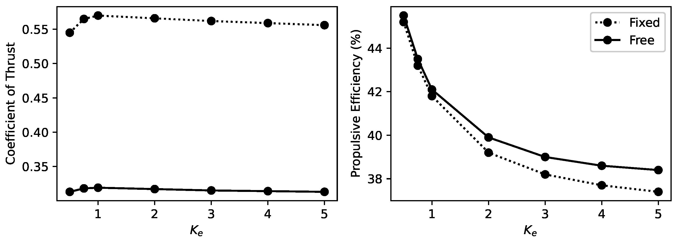
4.2. Effects of Flexibility

We investigate the impact of flexibility on the thrust coefficient and propulsive efficiency of a biomimetic batoid while maintaining consistent simulation parameters except for varying the elastic modulus value in Table 4 by introducing a stiffness scaling factor $K_e$. The results are depicted in Figure 15. From the graph, it is evident that the propulsive efficiency decreases monotonically with increasing stiffness, suggesting that a certain range of structural flexibility can be beneficial for improving propulsive efficiency. Conversely, the thrust coefficient initially increases and then decreases with increasing stiffness, implying that optimizing the stiffness of the pectoral fin to achieve maximum thrust is necessary.

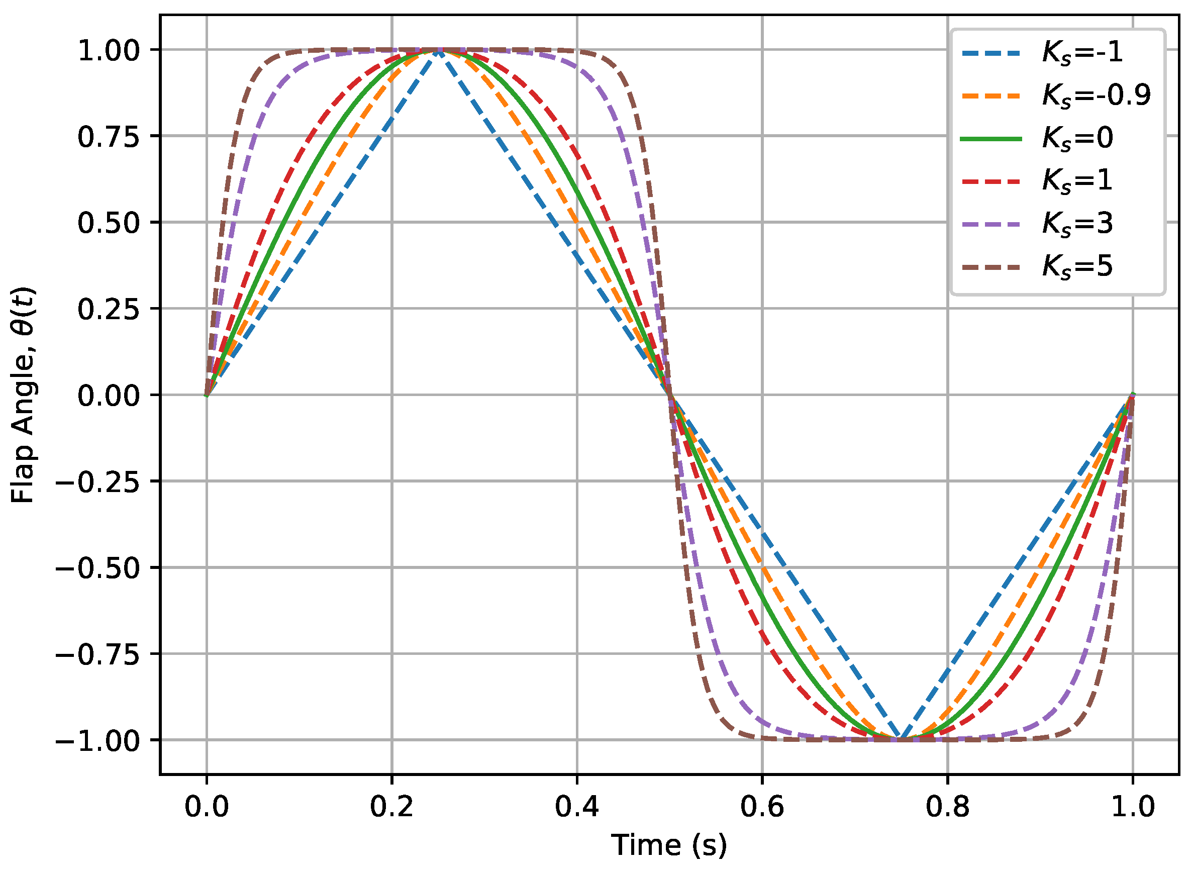
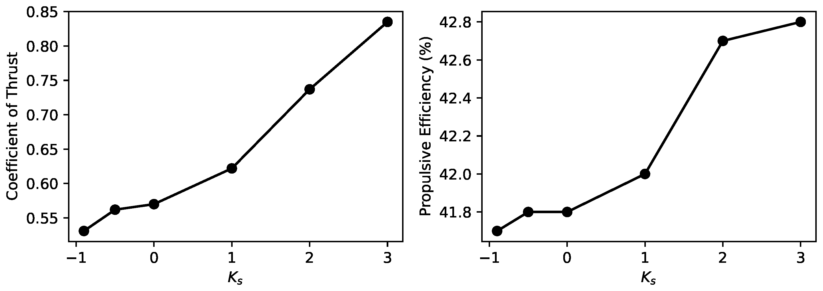
4.3. Effects of Non-Sinusoidal Flap Motion

Many aquatic animals, including manta rays, exhibit complex flapping angle $\theta$ variation processes that deviate from the commonly assumed sinusoidal curves in this paper and previous studies. To account for these non-sinusoidal patterns, we introduce an influence coefficient $K_s$ to gradually modify the standard sinusoidal waveform.

The proposed formula is as follows:

$$\theta \left(t\right)=\left\{\begin{array}{cc}{\displaystyle \frac{\theta arcsin(-K_{s}sin\left(2\pi ft\right))}{arcsin(-K_s)},}\hfill & -1\le K_s<0\hfill \\ \theta sin\left(2\pi ft\right),\hfill & K_s=0\hfill \\ {\displaystyle \frac{\theta tanh(K_{s}sin\left(2\pi ft\right))}{tanhK},}\hfill & K_s>0\hfill \end{array}\right.$$

(40)

Figure 16 illustrates the waveform diagrams for typical values of $K_s$. As $K_s$ increases, the sinusoidal waveform gradually transitions from a smooth curve to a square wave, while decreasing values of $K_s$ produce triangular waveforms.

The simulation outcomes obtained under varying coefficients $K_s$ are illustrated in Figure 17. It is evident that the triangular waveform is not advantageous for propulsion performance, as both the thrust coefficient and propulsive efficiency are inferior to those achieved with the sine wave. Conversely, the square waveform facilitates an enhancement in both the thrust coefficient and propulsive efficiency. The data suggests that within a certain range, the closer the approximation to a square wave, the more favorable the outcomes. This phenomenon could be attributed to the substantial derivative of the square waveform driving curve, which engenders a higher flapping velocity and consequently induces more potent vortices.

5. Self-Generated Vertical Undulations Analysis

5.1. Basic Analysis

In our previous simulation, we constrained the body as a boundary condition, neglecting the significant vertical force that accompanies the flapping motion of a mantabot due to water’s high density. In reality, this force induces vertical oscillations of the mantabot’s body during each flapping cycle. To better capture this phenomenon, we have relaxed the constraint on the body’s vertical motion, allowing it to oscillate up and down in response to the forces generated by the pectoral fin flapping. The remaining simulation parameters remain unchanged, as listed in Table 5. The resulting deformation and vortex particle trajectories within a flapping cycle are illustrated in Figure 18. The time series of the deformable body reveals a subtle up-and-down movement of the mantabot’s body, which, in turn, leads to a more extensive and curved distribution of the vortex particles in its wake. Notably, the simulation yields a thrust curve with an average thrust coefficient of 0.319, a 44% reduction compared to the fixed-vertical-freedom simulation, and an average propulsive efficiency of 42.1%, representing a 0.3% increase.

To explore why thrust significantly decreases when the vertical freedom is released, we analyzed the vortex structures following a complete flapping cycle of a biomimetic manta ray, as illustrated in Figure 19. By comparing this with the vortex structures observed when the vertical degrees of freedom are constrained, shown in Figure 11, we can identify two notable changes in the vortex dynamics due to the body’s undulating motion:

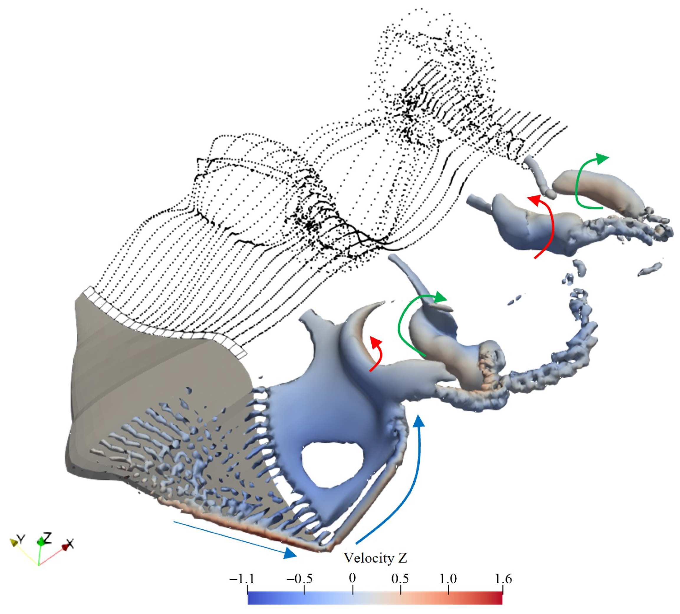
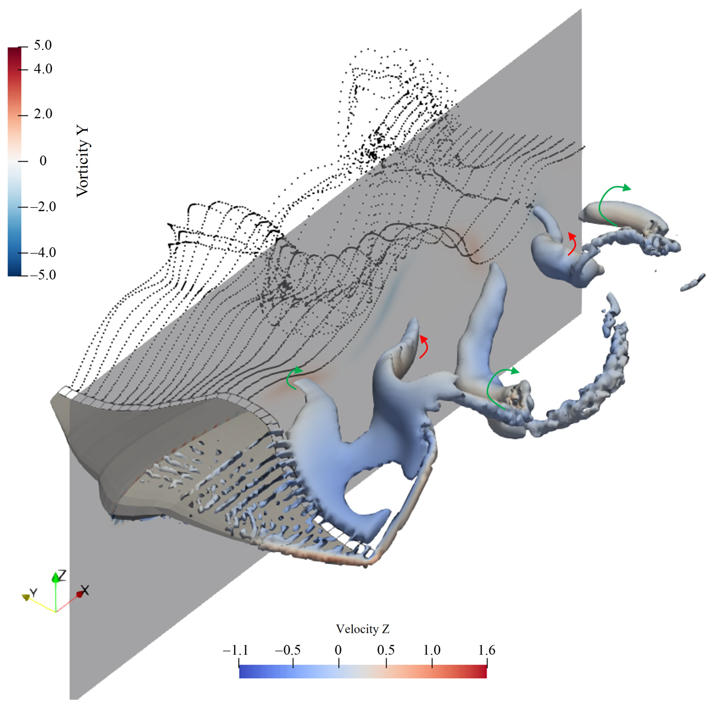
• The strength of the leading-edge vortex is significantly reduced, with a noticeable decrease in its coverage area near the body. This reduction leads to a diminished force exerted by the flow field on the structure;
• At the symmetry plane behind the body, the tail vortex exhibits stretching in the direction of the incoming flow, and its intensity is also diminished. This shift causes the location where the reverse Kármán vortex street typically forms to move backward. Given that the inductive effect of vortices follows an inverse square law, the farther from the body, the weaker the induced effect. As a result, the thrust generated by the reverse Kármán vortex street near the body is weakened.

These changes collectively result in a marked reduction in the propulsion force of the biomimetic manta ray.

5.2. Effects of Flexibility

To explore the influence of pectoral fin stiffness on propulsion when the body’s longitudinal movement is unrestricted, we replicated the simulation methodology outlined in Section 4.2, with results depicted in Figure 20. In the figure, the solid lines represent simulations with longitudinal freedom, while the dashed lines indicate scenarios with fixed longitudinal movement. The findings indicate an overall enhancement in the propulsive efficiency of the biomimetic manta ray across various conditions, accompanied by a reduction in the thrust coefficient, following a consistent trend. Further analysis shows that introducing longitudinal motion freedom diminishes the impact of pectoral fin stiffness on thrust generation. Specifically, the sensitivity of thrust to changes in structural stiffness decreases significantly. However, the decrease in sensitivity concerning propulsive efficiency, although present, is not markedly significant.

This suggests that optimizing structural stiffness with the sole aim of increasing thrust proves to be inefficient when the system operates under realistic conditions with longitudinal freedom. Given the diminished influence of structural stiffness on thrust in such scenarios, it would be more beneficial to focus on optimizing other aspects, such as the patterns of movement and the amplitude of fin flapping. This approach is likely to yield more substantial improvements in propulsion performance.

5.3. Effects of Non-Sinusoidal Flap Motion

We further explore whether the influence of non-sinusoidal flapping effects on propulsion is altered when the longitudinal degrees of freedom are released. As per the simulation settings outlined in Section 4.3, we only release the longitudinal degrees of freedom while maintaining all other conditions constant. The resulting simulation curves are depicted in Figure 21, where the solid line represents the outcomes with released longitudinal degrees of freedom, and the dashed line corresponds to those with fixed longitudinal degrees of freedom. It is observed that releasing the longitudinal degrees of freedom leads to a noticeable reduction in the thrust coefficient. However, the overall trend and the sensitivity of the curve to the non-sinusoidal coefficient remain nearly identical to the scenario with fixed longitudinal degrees of freedom. This finding is markedly different from the results discussed in Section 5.2, where releasing the longitudinal degrees of freedom resulted in a significant loss of sensitivity of the thrust coefficient to changes in structural stiffness. In terms of propulsive efficiency, the minimal variation suggests that the significant level of non-sinusoidal flapping defined in this study has a negligible impact on propulsive efficiency, irrespective of whether the longitudinal degrees of freedom are released.

5.4. Effects of Mass Distribution

In Section 5.2 and Section 5.3, we explored how structural rigidity and non-sinusoidal flapping dynamics influence propulsion, particularly under conditions that either restrict or permit longitudinal degrees of freedom. In addition to these scenarios, this section introduces another crucial variable only relevant when considering longitudinal freedom: the impact of mass distribution on propulsive efficiency.

We maintained the total mass of the biomimetic manta ray at 1 ton and analyzed changes in the thrust coefficient and propulsive efficiency across three different mass distributions, as detailed in

Table 6. Effects of different mass distribution on propulsion.

${\mathit{M}}_{\mathit{fins}}/{\mathit{M}}_{\mathit{body}}$	${\mathit{C}}_{\mathit{t}}$	Efficiency (%)
0.02	0.319	42.1
0.25	0.302	42.3
0.66	0.287	42.5

. The results demonstrate a decrease in the thrust coefficient when a larger portion of the mass is allocated from the body to the pectoral fins. This decrease becomes more pronounced as the proportion of mass in the body is reduced.

To visually compare the effects of different mass distributions, we plotted the longitudinal displacement curves for the three configurations on a single graph, shown in Figure 22. The solid line represents a scenario with a body mass of 1 ton and pectoral fin mass of 0.02 tons; the dashed line corresponds to a body mass of 0.8 tons and pectoral fin mass of 0.2 tons. In contrast, the dotted line illustrates the condition where the body’s buoyancy freedom is not considered. Different colors are used to distinguish between various spanwise positions.

The analysis revealed that with the inclusion of longitudinal degrees of freedom, the amplitude of longitudinal displacement decreases for the parts of the pectoral fins farther from the body, while it increases—and reverses direction—for the parts closer to the body. Importantly, an increased mass proportion in the pectoral fins significantly enhances the magnitude of longitudinal displacement for both the body and the proximal regions of the pectoral fins. This finding underscores the critical role of mass distribution in optimizing biomimetic designs for enhanced propulsive efficiency.

This finding indicates that to enhance thrust, it is crucial to reduce the structural mass of the pectoral fins in the design of biomimetic manta ray robots. A reduction in the structural mass necessitates simpler fin structures, suggesting that traditional methods, which often employ complex mechanical transmissions to mimic the swimming dynamics of manta rays, may not be optimal for these specific types of biomimetic robots. Consequently, the analysis of fluid–structure interactions, incorporating body degrees of freedom, will increasingly become critical in the development of sophisticated underwater biomimetic robotics.

6. Conclusions

Based on the simulation framework established in our previous study, this paper extends the model to include self-induced vertical undulations, providing a more realistic representation of the movement dynamics of biomimetic manta ray robots. The inclusion of these additional degrees of freedom has led to nuanced adjustments in the dynamics of propulsion, as evidenced by our comprehensive simulations and analyses. Below are the key findings and implications for the design and operation of biomimetic aquatic robots:

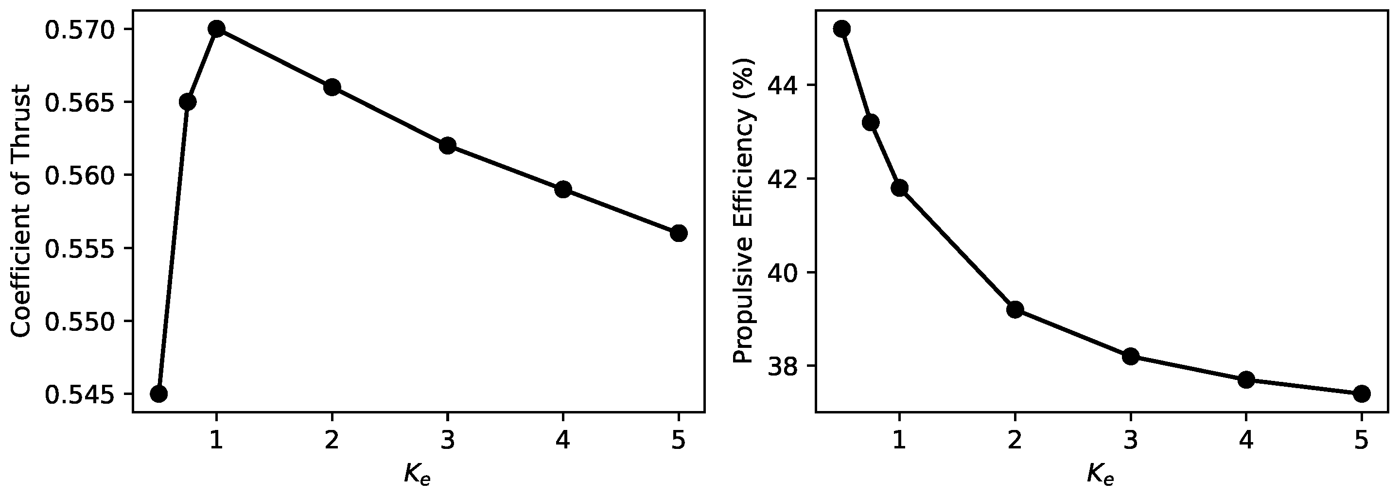
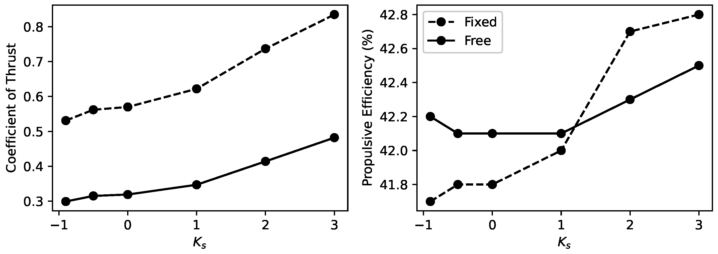
• The introduction of vertical freedom has notably diminished the influence of stiffness variations on thrust, resulting in a significant overall decrease in thrust. However, the propulsive efficiency shows a slight overall improvement, maintaining a consistent influence trend despite these changes.
• The adoption of a non-sinusoidal, square-wave flapping motion pattern brings us closer to the actual flapping motion of the manta ray, which significantly enhances thrust without substantially affecting propulsive efficiency. The impact of this motion pattern remains consistent even with the introduction of longitudinal degrees of freedom, suggesting a robust design strategy for enhancing propulsion.
• The distribution of mass is critically important in the design of biomimetic manta rays and has been largely overlooked in previous studies. An excessive focus on replicating the complex structure of the pectoral fins to mimic the real manta ray’s flapping motion has inadvertently increased the mass proportion of the pectoral fins. This, in turn, induces more pronounced longitudinal undulatory motions in the body, substantially reducing thrust.

While our study has focused on a constrained set of parameters, the results highlight the need for additional parametric research to refine design and operational tactics. The integrated dynamic framework for rigid body movement, elastic deformation, and fluid simulation introduced in this article showcases substantial utility and should be leveraged more frequently in the design and optimization of biomimetic underwater robots. This methodology not only deepens our comprehension of the underlying dynamics at play but also facilitates the tangible development of more effective and resilient aquatic robots.

Moreover, while this investigation has taken into account the vertical motion of the body resulting from pectoral fin flapping, the accompanying pitch motion has not been fully explored. This aspect of the study is left for future research to address, aiming to provide a more comprehensive analysis of the multifaceted dynamics involved in underwater locomotion.

References

1. Salazar, R.; Campos, A.; Fuentes, V.; Abdelkefi, A. A review on the modeling, materials, and actuators of aquatic unmanned vehicles. Ocean. Eng. 2019, 172, 257–285. [Google Scholar] [CrossRef]
2. Li, G.; Chen, X.; Zhou, F.; Liang, Y.; Xiao, Y.; Cao, X.; Zhang, Z.; Zhang, M.; Wu, B.; Yin, S.; et al. Self-powered soft robot in the Mariana Trench. Nature 2021, 591, 66–71. [Google Scholar] [CrossRef]
3. Lamas, M.; Rodriguez, C. Hydrodynamics of biomimetic marine propulsion and trends in computational simulations. J. Mar. Sci. Eng. 2020, 8, 479. [Google Scholar] [CrossRef]
4. Babu Mannam, N.P.; Mahbub Alam, M.; Krishnankutty, P. Review of biomimetic flexible flapping foil propulsion systems on different planetary bodies. Results Eng. 2020, 8, 100183. [Google Scholar] [CrossRef]
5. Wei, Q.P.; Wang, S.; Dong, X.; Shang, L.J.; Tan, M. Design and Kinetic Analysis of a Biomimetic Underwater Vehicle with Two Undulating Long-fins. Acta Autom. Sin. 2013, 39, 1330–1338. [Google Scholar] [CrossRef]
6. He, J.; Cao, Y.; Huang, Q.; Pan, G.; Dong, X.; Cao, Y. Effects of bionic pectoral fin rays’ spanwise flexibility on forwarding propulsion performance. J. Mar. Sci. Eng. 2022, 10, 783. [Google Scholar] [CrossRef]
7. Liu, K.; Liu, X.; Huang, H. Scaling the self-propulsive performance of pitching and heaving flexible plates. J. Fluid Mech. 2022, 936, A9. [Google Scholar] [CrossRef]
8. Cao, Y.; Cao, Y.; Ma, S.; Li, X.; Qu, Y.; Cao, Y. Realization and Online Optimization for Gliding and Flapping Propulsion of a Manta Ray Robot. J. Mar. Sci. Eng. 2023, 11, 2173. [Google Scholar] [CrossRef]
9. Zhou, C.; Low, K.H. Better Endurance and Load Capacity: An Improved Design of Manta Ray Robot (RoMan-II). J. Bionic Eng. 2010, 7, S137–S144. [Google Scholar] [CrossRef]
10. Lu, Y.; Cao, Y.; Pan, G.; Huang, Q.; Dong, X.; Cao, Y. Effect of cross-joints fin on the thrust performance of bionic pectoral fins. J. Mar. Sci. Eng. 2022, 10, 869. [Google Scholar] [CrossRef]
11. Chew, C.M.; Lim, Q.Y.; Yeo, K.S. Development of propulsion mechanism for Robot Manta Ray. In Proceedings of the 2015 IEEE International Conference on Robotics and Biomimetics (ROBIO), Zhuhai, China, 6–9 December 2015; pp. 1918–1923. [Google Scholar] [CrossRef]
12. Chen, L.; Bi, S.; Cai, Y.; Cao, Y.; Pan, G. Design and experimental research on a bionic robot fish with tri-dimensional soft pectoral fins inspired by cownose ray. J. Mar. Sci. Eng. 2022, 10, 537. [Google Scholar] [CrossRef]
13. Liu, Q.; Chen, H.; Wang, Z.; He, Q.; Chen, L.; Li, W.; Li, R.; Cui, W. A manta ray robot with soft material based flapping wing. J. Mar. Sci. Eng. 2022, 10, 962. [Google Scholar] [CrossRef]
14. Xing, C.; Cao, Y.; Cao, Y.; Pan, G.; Huang, Q. Asymmetrical Oscillating Morphology Hydrodynamic Performance of a Novel Bionic Pectoral Fin. J. Mar. Sci. Eng. 2022, 10, 289. [Google Scholar] [CrossRef]
15. Fish, F.; Schreiber, C.; Moored, K.; Liu, G.; Dong, H.; Bart-Smith, H. Hydrodynamic Performance of Aquatic Flapping: Efficiency of Underwater Flight in the Manta. Aerospace 2016, 3, 20. [Google Scholar] [CrossRef]
16. Zhang, Z.; Shi, L.; Guo, S.; Yin, H.; Li, A.; Bao, P.; Liu, M. Mechanism Design, Kinematic and Hydrodynamic Simulation of a Wave-driven Amphibious Robot. In Proceedings of the 2021 IEEE International Conference on Mechatronics and Automation (ICMA), Takamatsu, Japan, 8–11 August 2021; IEEE: Piscataway, NJ, USA, 2021; pp. 1038–1043. [Google Scholar]
17. Huang, H.; Sheng, C.; Jiannan, W.; Wu, G.; Zhou, C.; Wang, H. Hydrodynamic analysis and motion simulation of fin and propeller driven manta ray robot. Appl. Ocean. Res. 2021, 108, 102528. [Google Scholar] [CrossRef]
18. Qu, Y.; Xie, X.; Zhang, S.; Xing, C.; Cao, Y.; Cao, Y.; Pan, G.; Song, B. A Rigid-Flexible Coupling Dynamic Model for Robotic Manta with Flexible Pectoral Fins. J. Mar. Sci. Eng. 2024, 12, 292. [Google Scholar] [CrossRef]
19. Wang, W.; Huang, H.; Lu, X.Y. Interplay of chordwise stiffness and shape on performance of self-propelled flexible flapping plate. Phys. Fluids 2021, 33, 091904. [Google Scholar] [CrossRef]
20. Lapsansky, A.B.; Zatz, D.; Tobalske, B.W. Alcids ‘fly’at efficient Strouhal numbers in both air and water but vary stroke velocity and angle. eLife 2020, 9, e55774. [Google Scholar] [CrossRef] [PubMed]
21. Luo, M.; Wu, Z.; Yang, C. Strongly coupled fluid–structure interaction analysis of aquatic flapping wings based on flexible multibody dynamics and the modified unsteady vortex lattice method. Ocean. Eng. 2023, 281, 114921. [Google Scholar] [CrossRef]
22. Tasora, A.; Serban, R.; Mazhar, H.; Pazouki, A.; Melanz, D.; Fleischmann, J.; Taylor, M.; Sugiyama, H.; Negrut, D. Chrono: An Open Source Multi-physics Dynamics Engine. In High Performance Computing in Science and Engineering; Kozubek, T., Blaheta, R., Šístek, J., Rozložník, M., Čermák, M., Eds.; Springer International Publishing: Cham, Switzerland, 2016; Volume 9611, pp. 19–49. [Google Scholar] [CrossRef]
23. Recuero, A.; Negrut, D. Chrono Support for ANCF Finite Elements: Formulation and Validation Aspects; ResearchGate: Berlin, Germany, 2016. [Google Scholar]
24. Lee, H.; Sengupta, B.; Araghizadeh, M.; Myong, R. Review of vortex methods for rotor aerodynamics and wake dynamics. Adv. Aerodyn. 2022, 4, 20. [Google Scholar] [CrossRef]
25. Hess, J.L. The problem of three-dimensional lifting potential flow and its solution by means of surface singularity distribution. Comput. Methods Appl. Mech. Eng. 1974, 4, 283–319. [Google Scholar] [CrossRef]
26. TAN, J.; WANG, H.; WU, C.; LIN, C. Rotor/Empennage Unsteady Aerodynamic Interaction with Unsteady Panel/Viscous Vortex Particle Hybrid Method. Acta Aeronaut. Astronaut. Sin. 2014, 35, 14. [Google Scholar]
27. Tugnoli, M.; Montagnani, D.; Syal, M.; Droandi, G.; Zanotti, A. Mid-fidelity approach to aerodynamic simulations of unconventional VTOL aircraft configurations. Aerosp. Sci. Technol. 2021, 115, 106804. [Google Scholar] [CrossRef]
28. Dettmer, W.; Perić, D. A computational framework for fluid–rigid body interaction: Finite element formulation and applications. Comput. Methods Appl. Mech. Eng. 2006, 195, 1633–1666. [Google Scholar] [CrossRef]
29. Wendland, H. Piecewise polynomial, positive definite and compactly supported radial functions of minimal degree. Adv. Comput. Math. 1995, 4, 389–396. [Google Scholar] [CrossRef]
30. Wendland, H. Scattered Data Approximation; Cambridge University Press: Cambridge, UK, 2005. [Google Scholar]
31. Chourdakis, G.; Davis, K.; Rodenberg, B.; Schulte, M.; Simonis, F.; Uekermann, B.; Abrams, G.; Bungartz, H.; Cheung Yau, L.; Desai, I.; et al. preCICE v2: A sustainable and User-Friendly Coupling Library [Version 2; peer Review: 2 Approved]. Open Research Europe. 2022, Volume 2. Available online: https://open-research-europe.ec.europa.eu/articles/2-51/v2 (accessed on 1 June 2024).
32. Heathcote, S.; Wang, Z.; Gursul, I. Effect of spanwise flexibility on flapping wing propulsion. J. Fluids Struct. 2008, 24, 183–199. [Google Scholar] [CrossRef]
33. Masarati, P.; Morandini, M.; Quaranta, G.; Chandar, D.; Roget, B.; Sitaraman, J. Tightly Coupled CFD/Multibody Analysis of Flapping-Wing Micro-Aerial Vehicles. In Proceedings of the 29th AIAA Applied Aerodynamics Conference, Honolulu, HI, USA, 27–30 June 2011. [Google Scholar] [CrossRef]
34. Nakata, T.; Liu, H. A fluid–structure interaction model of insect flight with flexible wings. J. Comput. Phys. 2012, 231, 1822–1847. [Google Scholar] [CrossRef]
35. Xue, D.; Song, B.; Song, W.; Yang, W.; Xu, W.; Wu, T. Computational simulation and free flight validation of body vibration of flapping-wing MAV in forward flight. Aerosp. Sci. Technol. 2019, 95, 105491. [Google Scholar] [CrossRef]
36. Yang, S.b.; Qiu, J.; Han, X.y. Kinematics modeling and experiments of pectoral oscillation propulsion robotic fish. J. Bionic Eng. 2009, 6, 174–179. [Google Scholar] [CrossRef]
Figure 1. Multi-physics field coupling simulation classification diagram.
Jmse 12 01165 g001
Figure 2. (a) Aerial and aquatic flight trajectories of the Common murre, Uria aalge; (b) schematic diagram comparing actual and theoretical trajectories of flapping propulsion. Reproduced with permission from [20] published by eLife Sciences Publications Ltd., 2020.
Jmse 12 01165 g002
Figure 3. Surface and wake panels arrangements on wing and generation of vortex particles.
Jmse 12 01165 g003
Figure 4. Diagram of explicit coupling scheme and implicit coupling scheme.
Jmse 12 01165 g004
Figure 5. (a) Wing deformation and wake of the simulation model; (b) schematic of a spanwise flexible wing heaving periodically. Reproduced with permission from [32] published by Elsevier, 2008.
Jmse 12 01165 g005
Figure 6. (a) VPM simulated normalized displacements of leading-edge points across the span; (b) tip displacements from VPM, FLUENT, and experimental data.
Jmse 12 01165 g006
Figure 7. Manta-bot mesh and sections.
Jmse 12 01165 g007
Figure 8. Structural Skeleton of the Biomimetic Manta Robot.
Jmse 12 01165 g008
Figure 9. Variation of Flapping Angle and Flapping Angular Velocity over Simulation Time.
Jmse 12 01165 g009
Figure 10. Vortex particle wake and vorticity map during one flapping cycle of bionic manta ray pectoral fins.
Jmse 12 01165 g010
Figure 11. Isosurfaces of the Q-criterion (Q = 1.0) are shown to mark the vortex system at the end of the flapping cycle.
Jmse 12 01165 g011
Figure 12. Normalized vertical displacement of ribs and tip over time.
Jmse 12 01165 g012
Figure 13. Pitch Angle of ribs over time.
Jmse 12 01165 g013
Figure 14. Coefficient of thrust over time.
Jmse 12 01165 g014
Figure 15. Variation of thrust coefficient ( C T ) and propulsive efficiency ( η ) with stiffness coefficient ( K e ).
Jmse 12 01165 g015
Figure 16. The waveform diagrams of flap angle θ for typical values of K s .
Jmse 12 01165 g016
Figure 17. Variation of thrust coefficient ( C T ) and propulsive efficiency ( η ) with Non-sinusoidal coefficient ( K s ).
Jmse 12 01165 g017
Figure 18. (a) Side view of the displacement and deformation of a biomimetic mantabot during one flapping cycle; (b) Side view of the simulated vortex particle trace of the biomimetic mantabot.
Jmse 12 01165 g018
Figure 19. Isosurfaces of the Q-criterion (Q = 1.0) are shown to mark the vortex system at the end of the flapping cycle with vorticity map at the symmetric plane.
Jmse 12 01165 g019
Figure 20. Thrust coefficient ( C T ) and propulsive efficiency ( η ) vs. stiffness coefficient ( K e ) for fixed and free vertical undulations.
Jmse 12 01165 g020
Figure 21. Thrust coefficient ( C T ) and propulsive efficiency ( η ) vs. Non-sinusoidal coefficient ( K s ) for fixed and free vertical undulations.
Jmse 12 01165 g021
Figure 22. Normalized vertical displacement of body, ribs and tip over time.
Jmse 12 01165 g022